Embed Size (px)
Citation preview

Sustainability 2015, 7, 1-22; doi:10.3390/su7010001
sustainability ISSN 2071-1050
www.mdpi.com/journal/sustainability
Article
Spatiotemporal Changes of Farming-Pastoral Ecotone in Northern China, 1954–2005: A Case Study in Zhenlai County, Jilin Province
Yuanyuan Yang 1,2,3, Shuwen Zhang 1,2,*, Dongyan Wang 1, Jiuchun Yang 2 and Xiaoshi Xing 3
1 College of Earth Science, Jilin University, 2199 Jianshe Street, Changchun 130061, China;
E-Mails: [email protected] (Y.Y.); [email protected] (D.W.) 2 Northeast Institute of Geography and Agroecology, Chinese Academy Sciences,
4888 Shengbei Street, Changchun 130102, China; E-Mail: [email protected] 3 Center for International Earth Science Information Network (CIESIN), Earth Institute,
Columbia University, P.O. Box 1000 (61 Route 9W), Palisades, NY 10964, USA;
E-Mail: [email protected]
* Author to whom correspondence should be addressed; E-Mail: [email protected];
Tel.: +86-431-8554-2246.
Academic Editor: Vincenzo Torretta
Received: 3 June 2014 / Accepted: 12 December 2014 / Published: 23 December 2014
Abstract: Analyzing spatiotemporal changes in land use and land cover could provide basic
information for appropriate decision-making and thereby plays an essential role in promoting
the sustainable use of land resources, especially in ecologically fragile regions. In this paper,
a case study was taken in Zhenlai County, which is a part of the farming-pastoral ecotone of
Northern China. This study integrated methods of bitemporal change detection and temporal
trajectory analysis to trace the paths of land cover change for every location in the study area
from 1954 to 2005, using published land cover data based on topographic and environmental
background maps and also remotely sensed images including Landsat MSS (Multispectral
Scanner) and TM (Thematic Mapper). Meanwhile, the Lorenz curve and Gini coefficient
derived from economic models were also used to study the land use structure changes to gain
a better understanding of human impact on this fragile ecosystem. Results of bitemporal
change detection showed that the most common land cover transition in the study area was
an expansion of arable land at the expense of grassland and wetland. Plenty of grassland was
converted to other unused land, indicating serious environmental degradation in Zhenlai
County during the past decades. Trajectory analysis of land use and land cover change
OPEN ACCESS

Sustainability 2015, 7 2
demonstrated that settlement, arable land, and water bodies were relatively stable in terms
of coverage and spatial distribution, while grassland, wetland, and forest land had weak
stability. Natural forces were still dominating the environmental processes of the study area,
while human-induced changes also played an important role in environmental change.
In addition, different types of land use displayed different concentration trends and had large
changes during the study period. Arable land was the most decentralized, whereas forest land
was the most concentrated. The above results not only revealed notable spatiotemporal
features of land use and land cover change in the time series, but also confirmed the
applicability and effectiveness of the methodology in our research, which combined
bitemporal change detection, temporal trajectory analysis, and a Lorenz curve/Gini coefficient
in analyzing spatiotemporal changes in land use and land cover.
Keywords: spatiotemporal changes; land use and land cover change; land use structure;
sustainable use of land resources; farming-pastoral ecotone; northern China
1. Introduction
Decadal to centennial land use and land cover change (LUCC) has been widely singled out as an
integral component and important driver of global environmental change [1–4]. LUCC could
significantly affect key aspects of earth system functioning [5], playing an essential role in moving
towards global sustainability. A better understanding and quantification of past spatiotemporal
characteristics of land cover change as a fundamental ecological process is important in predicting the
development of future land use change and also in informing policy decisions on sustainable use of land
resource [6,7].
The farming-pastoral ecotone of Northern China is a sensitive region of terrestrial ecosystems and is
very vulnerable to global change and human disturbance. High-intensity human activities have produced
enormous negative environmental impacts in the region and the destruction of natural vegetation has
constantly drained the service functions of the local ecosystem service [8,9]. This ecotone is alarmingly
comparable to the Sahara region in northern Africa [10]. Zhenlai County, as a part of the farming-pastoral
ecotone of Northern China, is located in northwestern Jilin province, where the eco-environment is very
fragile and is vulnerable to disturbance from various factors. This area was widely covered by grassland
before the 1950s, when its eco-environment was relatively stable. After the People’s Republic of China
was formally established in 1949, soil salinization and grassland degradation became increasingly severe
owing to rapid population growth, excessive exploitation, and unreasonable land utilization [11]. Land
use structure in the study area has also undergone major changes. Arable, saline, and alkaline lands
increased significantly while grassland declined sharply [12–15]. Thus, the sustainable development of
the local socio-economy was greatly influenced. It is reported that the irrational land use structure has
led to low and unstable yields of arable land, and the severe land degradation has meant people in some
towns have poor living conditions [16]. In this context, the study of spatiotemporal changes and land use
structure changes over the past decades in Zhenlai County has become a significant topic.

Sustainability 2015, 7 3
Previous studies of spatiotemporal changes mainly focused on analyzing the categorical changes of
land cover with the accumulation of remotely sensed images using a bitemporal detection method [17–20].
The method in those studies analyzed land use and land cover change based on a two-epoch timescale.
In general, its application often requires measurements of the area’s ratio changes [21,22], the conversion
matrix of land cover change [23,24], and the spatial pattern changes characterized by land cover metrics
changes [25,26]. To study the human impact on the natural environment, it is often required to recover
the history of land cover change and to relate the spatiotemporal pattern of such change with other
environmental and human factors [27,28]. Rather than merely relying on the change of areas or other
indices, it is also important to effectively analyze the trends of land use and land cover change over time,
and to make clear the relationships between the factors that shape the changing nature of human–environment
dynamics and their effects within a particular region [28,29]. Trajectory analysis is a method of studying
and discovering trends in land cover change in the time series. Attempts have been made to apply a
trajectory analysis method on land use and land cover change in multiple time nodes [27–33]. Integrating
bitemporal change detection and temporal trajectory analysis could trace the paths of land cover change
for every location in an area.
In addition, land use structure could reflect the geographic configuration and comparison of land use
types. Analysis of land use structure could provide a better understanding of the relationship between
land use and the population-environment system, and also make clear the regional differences and
rationality of certain land use structures [34]. The Lorenz curve was an idea originally from economics
but has also been applied in many fields by using variables in relevant percentages for intuitive
distribution analysis. The Lorenz curve and associated Gini coefficient are simpler compared with
current study methods on land use structure, such as the artificial neural network (ANN) [35,36],
information entropy [37], optimal linear programming methods [38], and so on. The Lorenz curve and
Gini coefficient derived from economic models not only reveal the regularity of change in land use
structure and quantify the change process itself, but may also provide approaches for studying the
eco-environment [15,39,40].
Satellite images have been used extensively to study temporal changes in land use and land cover in
inaccessible areas of China where ground-truth data is lacking [17,18]. However, remotely-sensed data
have only existed for the last four decades at most, following the advent of the first land satellite,
LandSat-1, launched in 1972. Thus, most researchers could only do related studies in the past 30 years
due to the limits on available data. Understanding long-term human–environment interactions is essential
to understanding changes in terrestrial ecosystems [41,42]. Thus, it is necessary to study longer-term
spatiotemporal changes. This study seeks to use multitemporal satellite images and other data from
various sources to analyze spatiotemporal changes in Zhenlai County from 1954 to 2005. Our main
objectives are (1) to detect and to evaluate spatiotemporal changes in land use and land cover from 1954
to 2005 in the study area; (2) to trace the paths and to explore the trajectory of land cover change for
every location by integrating methods of bitemporal change detection and temporal trajectory analysis;
and (3) to analyze the regularity in land use structural changes and to gain a better understanding of
human impact on this fragile ecosystem by using the spatial Lorenz curve/Gini coefficient method.
Sustainability 2015, 7 4
2. Material and Methods
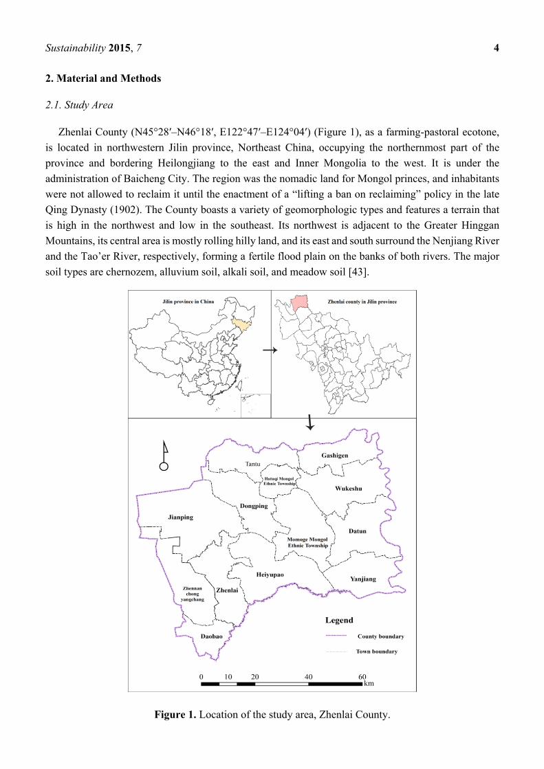
2.1. Study Area
Zhenlai County (N45°28′–N46°18′, E122°47′–E124°04′) (Figure 1), as a farming-pastoral ecotone,
is located in northwestern Jilin province, Northeast China, occupying the northernmost part of the
province and bordering Heilongjiang to the east and Inner Mongolia to the west. It is under the
administration of Baicheng City. The region was the nomadic land for Mongol princes, and inhabitants
were not allowed to reclaim it until the enactment of a “lifting a ban on reclaiming” policy in the late
Qing Dynasty (1902). The County boasts a variety of geomorphologic types and features a terrain that
is high in the northwest and low in the southeast. Its northwest is adjacent to the Greater Hinggan
Mountains, its central area is mostly rolling hilly land, and its east and south surround the Nenjiang River
and the Tao’er River, respectively, forming a fertile flood plain on the banks of both rivers. The major
soil types are chernozem, alluvium soil, alkali soil, and meadow soil [43].
Figure 1. Location of the study area, Zhenlai County.
Sustainability 2015, 7 5
Climatically, the region is subject to a temperate continental monsoon climate with distinct seasons,
as it is located in inland areas of mid-latitude. The mean annual rainfall is 402.4 mm, unevenly
distributed over time, while the mean annual evaporation is 1755.9 mm, about four times as high as the
mean annual rainfall. Thus, the low amount of precipitation and the high amount of evaporation mainly
result in a drought-prone climate in the study area, especially in spring. The mean annual temperature is
around 4.9 °C [43].
2.2. Data
Based on our former study about the LUCC rate and the available data in the study area, monitoring
of land use and land cover changes was done at four time nodes: 1954, 1976, 2000, and 2005. One
Landsat MSS (Multispectral Scanner) and two Landsat TM (Thematic Mapper) images were selected
pertaining to the years 1976, 2000, and 2005. Meanwhile, our research team reconstructed the
spatiotemporal distribution of land use and land cover in 1954 by making use of topographic maps and
physical environmental background maps including those of terrain, climate, geology, soil, vegetation,
hydrology, and socioeconomic statistical data. The digital reconstruction model of land use was built
based on the cellular automata (CA) model. It consists of five modules: spatial analysis module,
sensitivity analysis module, diagnostic module for arable land distribution, demand analysis module,
and spatial layout module [44,45].
2.3. Classification System
For comparisons over time, the maps had to be thematically generalized. Taking into account both
the local characteristics and the predominant land use classification system used in China [46], the
available land classes were aggregated into seven suitable land categories for this study: arable land
(including paddy fields and rainfed cropland); forest land (including deciduous forest, coniferous forest,
low pinewood, orchards, etc.); grassland (including natural grassland and pasture); water bodies
(including rivers, lakes, and ponds); settlement (urban and rural construction); wetland; and other unused
land (including sand, saline-alkali land, and bare land).
2.4. Methods
2.4.1. Transition Probabilities Matrix for Land Use/Land Cover Dynamics
Within the region of interest we assume a spatially homogeneous probability of transition from one
land class to another between time t and time t+1. Denote the area of land which switches from class i to class j between time t and t+1 by t
ijS , and the area of land in class i at time t by t
iS . Then the
probability of transition from land class i to land class j by t
ijP is estimated as the ratio of these two
quantities as follows:
/t t tij ij iP S S
(1)
However, the above transition probability for land use cannot allow us to fully understand land use
change as land use change among various land cover types often has the inverse transition during

Sustainability 2015, 7 6
different time intervals. In this situation, the concept of cumulative transition probability for land
use [47,48] is proposed as in Formula (2):
1
( / ) 100%n
tij ij T
t
P S S
(2)
where ijP is the cumulative transition probability for land use from category i to j during the entire study
period; i and j are the land use types; tijS is the conversion area from category i to j during the time
interval t and t+1; n is the number of time intervals; and TS is the total of the study area.
2.4.2. Trajectory Computing Method
Change trajectory of the time series can be expressed by trajectory codes in the form of figures or
letters for every parcel in the vector layer [28,30,33]. The numeric code could be operated and calculated
in the software ArcGIS, while the letter codes could be used clearly to identify the land use type in the
trajectory analysis. Thus, we firstly used the numeric codes to calculate the trajectory of land use change
in ArcGIS, and then used the letter codes to analyze the change trajectory. In this study, the following
figures were used to stand for each land category for each layer of time node in the trajectory analysis:
“1” stands for “Arable land”; “2” stands for “Forest land”; “3” stands for “Grassland”; “4” stands for
“Water”; “5” stands for “Settlement”; “6” stands for “Wetland”; and “7” stands for “Other unused land”.
Trajectory codes for each parcel can be obtained using Formula (3) as below:
1 2( 1) 10 ( 2) 10 ... ( ) 10n n n ni i i iY G G Gn (3)
where Yi is the trajectory code of the parcel i in the trajectory layer; n is the number of time nodes; and
(G1)i, (G2)i, and (Gn)i are the codes of the land use/cover type of each time node at the given parcel.
Thus, the trajectory codes (e.g., 3631, 1333) of every parcel can be calculated automatically. Then,
we used the following letter codes to replace the numeric codes: “A” stands for “Arable land”; “F” stands
for “Forest land”; “G” stands for “Grassland”; “W” stands for “Water”; “S” stands for “Settlement”;
“M” stands for “Wetland”; and “O” stands for “Other unused land”. In addition, we used the symbol
“→” to show the change direction in time series. Thus, the above trajectory codes “3631” would be
replaced by “G→M→G→A”, which means that the land was found to be grassland in 1954, wetland in
1956, grassland again in 2000, and cultivated as arable land in 2005; “1333” would be replaced by
“A→G→G→G”, which means that the land was found to be arable land in 1954 and abandoned as
grassland in 1976, 2000, and 2005. Not only can the land use/cover change for every parcel and every
time node in the study area be shown in the trajectory codes, but also the trajectory for every parcel
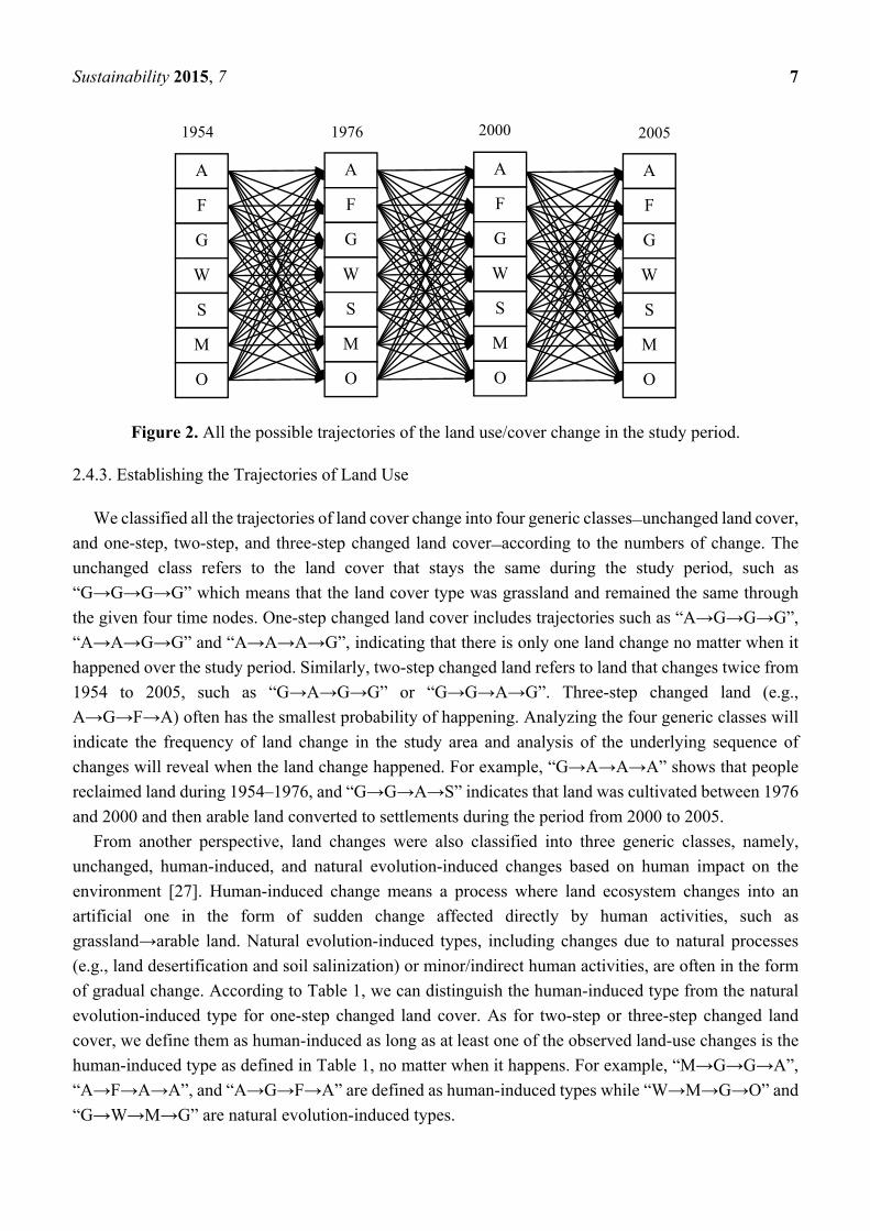
through the time series can be specified by land categories (Figure 2).
Sustainability 2015, 7 7
Figure 2. All the possible trajectories of the land use/cover change in the study period.
2.4.3. Establishing the Trajectories of Land Use
We classified all the trajectories of land cover change into four generic classes—unchanged land cover,
and one-step, two-step, and three-step changed land cover—according to the numbers of change. The
unchanged class refers to the land cover that stays the same during the study period, such as
“G→G→G→G” which means that the land cover type was grassland and remained the same through
the given four time nodes. One-step changed land cover includes trajectories such as “A→G→G→G”,
“A→A→G→G” and “A→A→A→G”, indicating that there is only one land change no matter when it
happened over the study period. Similarly, two-step changed land refers to land that changes twice from
1954 to 2005, such as “G→A→G→G” or “G→G→A→G”. Three-step changed land (e.g.,
A→G→F→A) often has the smallest probability of happening. Analyzing the four generic classes will
indicate the frequency of land change in the study area and analysis of the underlying sequence of
changes will reveal when the land change happened. For example, “G→A→A→A” shows that people
reclaimed land during 1954–1976, and “G→G→A→S” indicates that land was cultivated between 1976
and 2000 and then arable land converted to settlements during the period from 2000 to 2005.
From another perspective, land changes were also classified into three generic classes, namely,
unchanged, human-induced, and natural evolution-induced changes based on human impact on the
environment [27]. Human-induced change means a process where land ecosystem changes into an
artificial one in the form of sudden change affected directly by human activities, such as
grassland→arable land. Natural evolution-induced types, including changes due to natural processes
(e.g., land desertification and soil salinization) or minor/indirect human activities, are often in the form
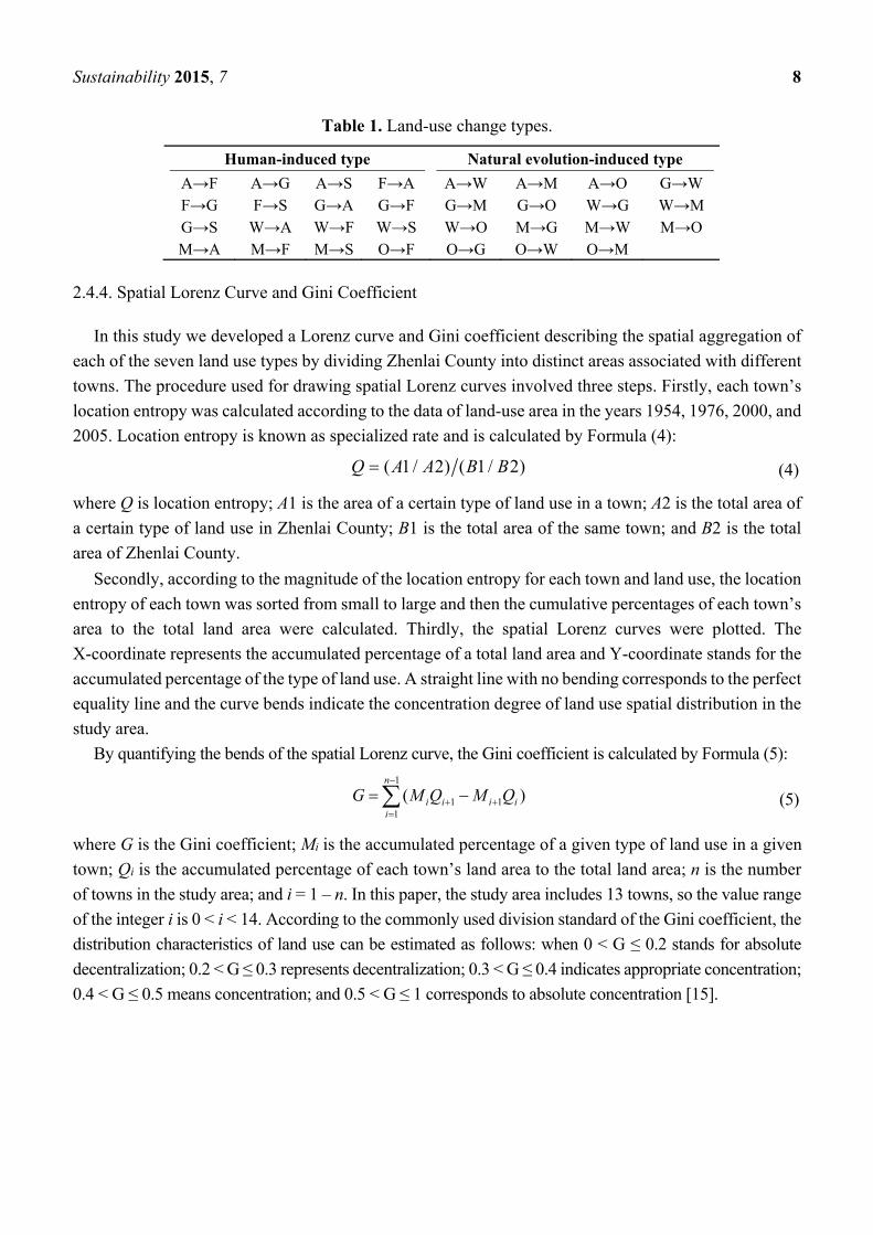
of gradual change. According to Table 1, we can distinguish the human-induced type from the natural
evolution-induced type for one-step changed land cover. As for two-step or three-step changed land
cover, we define them as human-induced as long as at least one of the observed land-use changes is the
human-induced type as defined in Table 1, no matter when it happens. For example, “M→G→G→A”,
“A→F→A→A”, and “A→G→F→A” are defined as human-induced types while “W→M→G→O” and
“G→W→M→G” are natural evolution-induced types.
A
F
G
W
S
M
O
1954
A
F
G
W
S
M
O
1976
A
F
G
W
S
M
O
2000
A
F
G
W
S
M
O
2005
Sustainability 2015, 7 8
Table 1. Land-use change types.
Human-induced type Natural evolution-induced type
A→F A→G A→S F→A A→W A→M A→O G→W F→G F→S G→A G→F G→M G→O W→G W→M G→S W→A W→F W→S W→O M→G M→W M→O M→A M→F M→S O→F O→G O→W O→M
2.4.4. Spatial Lorenz Curve and Gini Coefficient
In this study we developed a Lorenz curve and Gini coefficient describing the spatial aggregation of
each of the seven land use types by dividing Zhenlai County into distinct areas associated with different
towns. The procedure used for drawing spatial Lorenz curves involved three steps. Firstly, each town’s
location entropy was calculated according to the data of land-use area in the years 1954, 1976, 2000, and
2005. Location entropy is known as specialized rate and is calculated by Formula (4):
( 1 / 2) ( 1 / 2)Q A A B B (4)
where Q is location entropy; A1 is the area of a certain type of land use in a town; A2 is the total area of
a certain type of land use in Zhenlai County; B1 is the total area of the same town; and B2 is the total
area of Zhenlai County.
Secondly, according to the magnitude of the location entropy for each town and land use, the location
entropy of each town was sorted from small to large and then the cumulative percentages of each town’s
area to the total land area were calculated. Thirdly, the spatial Lorenz curves were plotted. The
X-coordinate represents the accumulated percentage of a total land area and Y-coordinate stands for the
accumulated percentage of the type of land use. A straight line with no bending corresponds to the perfect
equality line and the curve bends indicate the concentration degree of land use spatial distribution in the
study area.
By quantifying the bends of the spatial Lorenz curve, the Gini coefficient is calculated by Formula (5):
)(1
111
n
iiiii QMQMG (5)
where G is the Gini coefficient; Mi is the accumulated percentage of a given type of land use in a given
town; Qi is the accumulated percentage of each town’s land area to the total land area; n is the number
of towns in the study area; and i = 1 – n. In this paper, the study area includes 13 towns, so the value range
of the integer i is 0 < i < 14. According to the commonly used division standard of the Gini coefficient, the
distribution characteristics of land use can be estimated as follows: when 0 < G ≤ 0.2 stands for absolute
decentralization; 0.2 < G ≤ 0.3 represents decentralization; 0.3 < G ≤ 0.4 indicates appropriate concentration;
0.4 < G ≤ 0.5 means concentration; and 0.5 < G ≤ 1 corresponds to absolute concentration [15].

Sustainability 2015, 7 9
3. Results and Discussion
3.1. Land Use and Land Cover Change (1954–2005)
3.1.1. Temporal Properties
It was found that the land use/cover changed significantly after statistical analysis of the land-use area
over the study period in Zhenlai County (Table 2 and Figure 3). In 1954–2005, arable land, grassland,
and wetland were the dominant land use types, with over 70% of total area percentage. Arable land,
forest, and settlement expanded continuously from 1954 to 2005 (Figure 4). It is especially important to
note that arable land had the largest increase, from 31.48% in 1954 to 39.07% in 2005, while both
grassland and wetland had significant loss during the past 60 years. In 1954, grassland and wetland
occupied 30.54% and 32.26% of the total study area; however, these areas had declined to 12.27% and
18.81%, respectively, by 2005. The proportional area of water bodies changed slightly, fluctuating from
4.89% in 1954 to 5.50% in 2005. Water bodies were mainly influenced by natural factors, especially
affected by climate change in the absence of irrigation facilities such as reservoirs. Other unused land
surged from 1954 to 1976 and continued to increase until 2000, and then it began to decline slightly as
people started to emphasize controlling desertification and salinization.
Figure 3. Percentage of area of each land category, 1954–2005.
0.00
10.00
20.00
30.00
40.00
Arable land Forest land Grassland Water settlement Wetland Other unusedland
1954 1976 2000 2005
Are
a pe
rcen
tage
(%
)

Sustainability 2015, 7 10
Table 2. Area and percentage changes during the time intervals.
Categories
Area (in ha) and percentages (%) Changes (in ha)
1954 1976 2000 2005 1954–1976 1976–2000 2000–2005
Area % Area % Area % Area %
Arable land 16,7355.69 31.48 19,2533.35 36.22 198,950.45 37.42 207,717.83 39.07 25,177.66 6417.10 8767.38 Forest land 488.65 0.09 12,117.17 2.28 19,065.53 3.59 18,900.88 3.56 11,628.51 6948.36 –164.65 Grassland 16,2371.84 30.54 88,892.09 16.72 60,215.14 11.33 65,223.77 12.27 −73,479.75 −28,676.94 5008.63
Water 26,000.01 4.89 29,352.35 5.52 30,024.12 5.65 29,259.09 5.50 3352.34 671.78 –765.03 Settlement 2944.58 0.55 11,109.70 2.09 12,503.21 2.35 12,547.33 2.36 8165.12 1393.51 44.12 Wetland 17,1500.15 32.26 111,101.27 20.90 107,753.65 20.27 99,975.96 18.81 −60,398.88 –3347.62 −7777.69
Other unused land
945.22 0.18 86,500.22 16.27 103,094.04 19.39 97,981.28 18.43 85,555.01 16,593.82 −5112.76
(a) (b) (c) (d)
Figure 4. Land use/cover maps for the years (a) 1954; (b) 1976; (c) 2000 and (d) 2005.

Sustainability 2015, 7 11
3.1.2. Bitemporal Change Detection
A transition matrix was used to summarize the state of each land use in each time interval and the
transitions through time with respect to each land category. From Tables 3 and 4, and Figure 5, the
results indicated that arable land expanded at the expense of grassland and wetland. Grassland had the
largest cumulative transition probability (34.37%) during the period from 1954 to 2005, and 15.41% of
grassland was changed into arable land while 15.02% of grassland was converted to wetland and other
unused land. However, from 1954 to 1976, 38.90% of grassland was turned into arable land due to the
fast growth of the population (from 145,328 persons in 1954 to 277,146 persons in 1976). Furthermore,
24.20% of grassland was converted to other unused land during 1976–2000, indicating serious
environmental degradation. Wetland had the second largest cumulative transition probability (32.90%)
during the study period. Wetland was mainly changed into arable land and other unused land, reflecting
both human activities and natural processes affected by the climate. Wetland was changed to arable land
with similar transition probabilities during the three time intervals from 1954 to 1976 (11.79%), 1976 to
2000 (16.75%), and 2000 to 2005 (15.45%). Also, 33.35% of wetland was changed to other unused land
between 1954 and 1976. In addition, abandoned land could not be ignored during the study area. The
cumulative transition probability of arable land is 26.20%, ranking third.
Table 3. Transition probability matrices of land changes in each period (%).
Categories Period Arable
land
Forest
land Grassland Water Settlement Wetland
Other unused
land
Arable
land
1954–1976 56.19 3.74 15.58 2.01 5.55 8.51 8.42
1976–2000 81.27 1.80 2.91 0.10 2.84 11.05 0.04
2000–2005 84.97 5.87 0.00 0.00 9.16 0.00 0.00
Forest land
1954–1976 12.99 21.04 57.91 0.00 5.26 2.81 0.00
1976–2000 19.93 79.80 0.00 0.00 0.26 0.00 0.00
2000–2005 15.86 84.14 0.00 0.00 0.00 0.00 0.00
Grassland
1954–1976 38.90 3.96 18.28 2.25 1.15 24.55 10.90
1976–2000 10.11 9.83 54.66 0.23 0.13 0.84 24.20
2000–2005 16.19 0.00 83.81 0.00 0.00 0.00 0.00
Water
1954–1976 5.89 0.19 4.78 41.97 0.14 25.16 21.87
1976–2000 2.50 2.50 2.50 85.00 2.50 2.50 2.50
2000–2005 1.39 0.00 3.15 70.41 0.00 23.33 1.72
Settlement
1954–1976 36.31 0.79 5.91 0.82 42.04 3.76 10.37
1976–2000 2.50 2.50 2.50 2.50 85.00 2.50 2.50
2000–2005 2.50 2.50 2.50 2.50 85.00 2.50 2.50
Wetland
1954–1976 11.79 0.58 20.15 6.02 0.41 27.70 33.35
1976–2000 16.75 0.00 4.05 0.83 0.00 77.86 0.52
2000–2005 15.45 0.00 0.25 8.68 0.00 75.62 0.00
Other
unused
land
1954–1976 0.44 0.00 1.14 85.29 0.00 7.53 5.60
1976–2000 0.69 0.00 0.00 3.20 0.33 11.33 84.44
2000–2005 0.09 0.00 18.64 0.55 0.00 0.19 80.53

Sustainability 2015, 7 12
Table 4. Cumulative transition probabilities (%).
1954–2005 Arable
land Forest land
Grassland Water Settlement Wetland Other
unused land Total
Arable land 0.00 4.03 5.96 0.67 6.20 6.68 2.67 26.20Forest land 1.04 0.00 0.05 0.00 0.01 0.00 0.00 1.10 Grassland 15.41 2.85 0.00 0.73 0.37 7.64 7.38 34.37
Water 0.50 0.15 0.55 0.00 0.14 2.69 1.30 5.34 Settlement 0.31 0.12 0.14 0.12 0.00 0.13 0.17 0.99 Wetland 10.44 0.19 7.40 3.87 0.13 0.00 10.87 32.90
Other unused land 0.13 0.00 3.62 0.78 0.05 1.89 0.00 6.47
Figure 5. Cumulative transition areas from 1954 to 2005 (×10,000 ha).
3.1.3. Spatial Distributions and Trajectories of Land Cover Change
During the study period, unchanged land occupied 35.83% of the total area, and one-step, two-step,
and three-step changed land occupied 55.54%, 8.07%, and 0.56%, respectively. Taking land use data in
1954 as a baseline, 64.80% of arable land, 49.33% of settlement, and 44.91% of water bodies remained
the same during the study period (Table 5), indicating that these land categories had relatively strong
stability and certainty in the spatial distributions.
Table 5. Percentages of unchanged land areas to the corresponding land areas in 1954 by types (%):
A = Arable land; F = Forest land; G = Grassland; W = Water; S = Settlement; M = Wetland;
O = Other unused land.
Unchanged land use
% Unchanged
land use %
Unchanged land use
% Unchanged
land use %
A 64.80 F 24.97 G 13.53 W 44.91S 49.33 M 27.26 O 6.88
Arable land
ForestlandGrassland
WaterSettlement
WetlandOther unused land
0
1
2
3
4
5
6
7
8
Ara
ble
land
For
estl
and
Gra
ssla
nd
Wat
er
Set
tlem
ent
Wet
land
Oth
er u
nuse
d la
nd
Arable land
Forestland
Grassland
Water
Settlement
Wetland
Other unused land
×10,000 ha
to
from

Sustainability 2015, 7 13
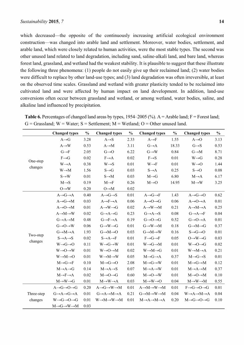
There were 34 types of one-step land changes (Table 6), mainly including grassland→arable land
(18.33%), wetland→other unused land (14.95%), grassland→wetland (8.71%), wetland→grassland
(6.80%), grassland→other unused land (6.22%), and wetland→arable land (6.17%). The rest of the one-
step changes were less than 4%. Moreover, among these one-step changed trajectories, “G→A→A→A”
contributed the largest percentage (16.80% of the total changed land area from 1954 to 2005), while
“G→G→A→A” and “G→G→G→A” contributed the percentages of 1.50% and 0.03%, respectively.
The percentages of “M→A→A→A”, “M→M→A→A” and “M→M→M→A” contributed 4.74%,
0.89%, and 0.54%, respectively. The above analyses illustrated that people reclaimed and cultivated land
intensely during 1954–1976, creating the dominant effect on land use. This could be driven by the
national macro-policy actively encouraging people to reclaim and farm to develop local agriculture. The
adjustment of production relations mobilized people’s enthusiasm to reclaim land since the 1950s [49,50].
One-step changes showed that once one land type was changed to another, it would then reach a steady
state. For example, two-step changed land use would not occur if a quantity of grassland was changed
into arable land. This might illustrate that people would not easily give up their reclaimed land unless an
irresistible force exists. “Wetland→Other unused land” indicated that land degradation has difficult
reversibility. Moreover, there were many conversions between grassland and wetland for the following
two reasons: (1) wetland had a clear relationship with precipitation and would be changed into grassland
in the years with less precipitation; (2) there were plenty of lakes and ponds inside and surrounding the
Nenjiang River and the Tao’er River to the east and south of the study area, respectively, which made
the nearby wetland, grassland, and other unused land convert frequently.
There were 60 types of two-step changes, mainly including wetland→grassland→other unused land
(2.08%), grassland→wetland→arable land (1.93%), and arable land→grassland→forest land (1.43%).
However, there were only 13 types of three-step changes, all with small percentages of the areas.
Altogether, the analysis of two-step and three-step changes showed that arable land, grassland, wetland,
water bodies, and other unused land were converted frequently; this may be due to the influence
of rainfall.
Figure 6c shows that the trajectory analysis of land cover can display the histories of land use change
and their features related to different driving forces over the study period. During the 60-year study
period, unchanged land occupied 35.83% of the total area, human-induced changes occupied 26.89%,
and natural evolution land area occupied 37.28%, respectively. In the study area, human-induced
changes were mainly distributed in two areas, namely, cultivation in the northwest and east along the
Nenjiang River. Unchanged, natural, and human-induced land use appeared stepwise from east (along
the Nenjiang River) to west. Natural change along the Nenjiang River was likely to be caused by the
fluctuation between flooding and drying. The fertile flood plain on the river’s banks allowed the land to
be cultivated easily and produce a high grain yield.
From 1954 to 2005, once unchanged land and the land influenced by natural type were subject to
human-induced changes, they tended to reach stability and were less likely to change in the following
time nodes. In contrast, areas where changes were once influenced by natural evolution were more likely
to change further. A plausible explanation for this is that land cover tends to be changed into a certain
type that could increase its value or improve quality due to human activities. If it is converted into another
type, the land value tends to decline or the switching cost tends to increase. Thus, it sometimes may
drastically reduce the possibility that the land is used for other purposes. Analysis found that grassland,
Sustainability 2015, 7 14
which decreased—the opposite of the continuously increasing artificial ecological environment
construction—was changed into arable land and settlement. Moreover, water bodies, settlement, and
arable land, which were closely related to human activities, were the most stable types. The second was
other unused land related to land degradation, including sand, saline-alkali land, and bare land, whereas
forest land, grassland, and wetland had the weakest stability. It is plausible to suggest that these illustrate
the following three phenomena: (1) people do not easily give up their reclaimed land; (2) water bodies
were difficult to replace by other land-use types; and (3) land degradation was often irreversible, at least
on the observed time scales. Grassland and wetland with greater plasticity tended to be reclaimed into
cultivated land and were affected by human impact on land development. In addition, land-use
conversions often occur between grassland and wetland, or among wetland, water bodies, saline, and
alkaline land influenced by precipitation.
Table 6. Percentages of changed land areas by types, 1954–2005 (%). A = Arable land; F = Forest land;
G = Grassland; W = Water; S = Settlement; M = Wetland; O = Other unused land.
Changed types % Changed types % Changed types % Changed types %
One-step
changes
A→G 3.28 A→S 2.33 A→F 1.55 A→O 3.13
A→W 0.53 A→M 3.11 G→A 18.33 G→S 0.53
G→F 2.05 G→O 6.22 G→W 0.84 G→M 8.71
F→G 0.02 F→A 0.02 F→S 0.01 W→G 0.28
W→A 0.38 W→S 0.01 W→F 0.01 W→O 1.44
W→M 1.56 S→G 0.03 S→A 0.25 S→O 0.08
S→W 0.01 S→M 0.03 M→G 6.80 M→A 6.17
M→S 0.19 M→F 0.26 M→O 14.95 M→W 3.25
O→W 0.20 O→M 0.02
Two-step
changes
A→G→A 0.40 A→G→S 0.01 A→G→F 1.43 A→G→O 0.62
A→G→M 0.03 A→F→A 0.06 A→O→G 0.06 A→O→A 0.01
A→O→M 0.01 A→W→G 0.02 A→W→M 0.21 A→M→A 0.25
A→M→W 0.02 G→A→G 0.23 G→A→S 0.08 G→A→F 0.04
G→A→M 0.48 G→F→A 0.19 G→O→G 0.52 G→O→A 0.01
G→O→W 0.06 G→W→G 0.01 G→W→M 0.18 G→M→G 0.37
G→M→A 1.93 G→M→O 0.03 G→M→W 0.16 S→G→O 0.01
S→A→S 0.02 S→A→F 0.01 F→G→F 0.05 O→W→G 0.03
W→G→O 0.11 W→G→W 0.01 W→G→M 0.01 W→O→G 0.02
W→O→W 0.01 W→O→M 0.02 W→M→G 0.01 W→M→A 0.21
W→M→O 0.01 W→M→W 0.05 M→G→A 0.37 M→G→S 0.01
M→G→F 0.10 M→G→O 2.08 M→G→W 0.01 M→G→M 0.12
M→A→G 0.14 M→A→S 0.07 M→A→W 0.01 M→A→M 0.37
M→F→A 0.02 M→O→G 0.60 M→O→W 0.01 M→O→M 0.10
M→W→G 0.01 M→W→A 0.03 M→W→O 0.04 M→W→M 0.55
Three-step
changes
A→G→O→G 0.20 A→G→W→M 0.01 A→M→W→M 0.01 F→G→O→G 0.01
G→A→G→A 0.01 G→A→M→A 0.21 G→M→W→M 0.04 W→A→M→A 0.04
W→G→O→G 0.01 W→M→W→M 0.01 M→A→M→A 0.20 M→G→O→G 0.10
M→G→W→M 0.03

Sustainability 2015, 7 15
(a)
(b)
(c)
Figure 6. Trajectories of unchanged land use (a) and land use changes (b,c), 1954–2005.
3.2. Land Use Structure
The spatial Lorenz curves for the various land use types are shown in Figure 7. The spatial Lorenz
curves of arable land are always the nearest to the perfect equality line in the study period, those of
settlement are second, and those of grassland are third. Land curves of forest are always the farthest.
These characteristics illustrate that arable land showed the most decentralized distribution among the
seven land use types, followed by settlement and grassland. Meanwhile, forest land exhibited the most
concentrated distribution, especially in 1954. Water bodies, wetland, and other unused land had different
characteristics and showed distinct concentrated distribution at the four time nodes.
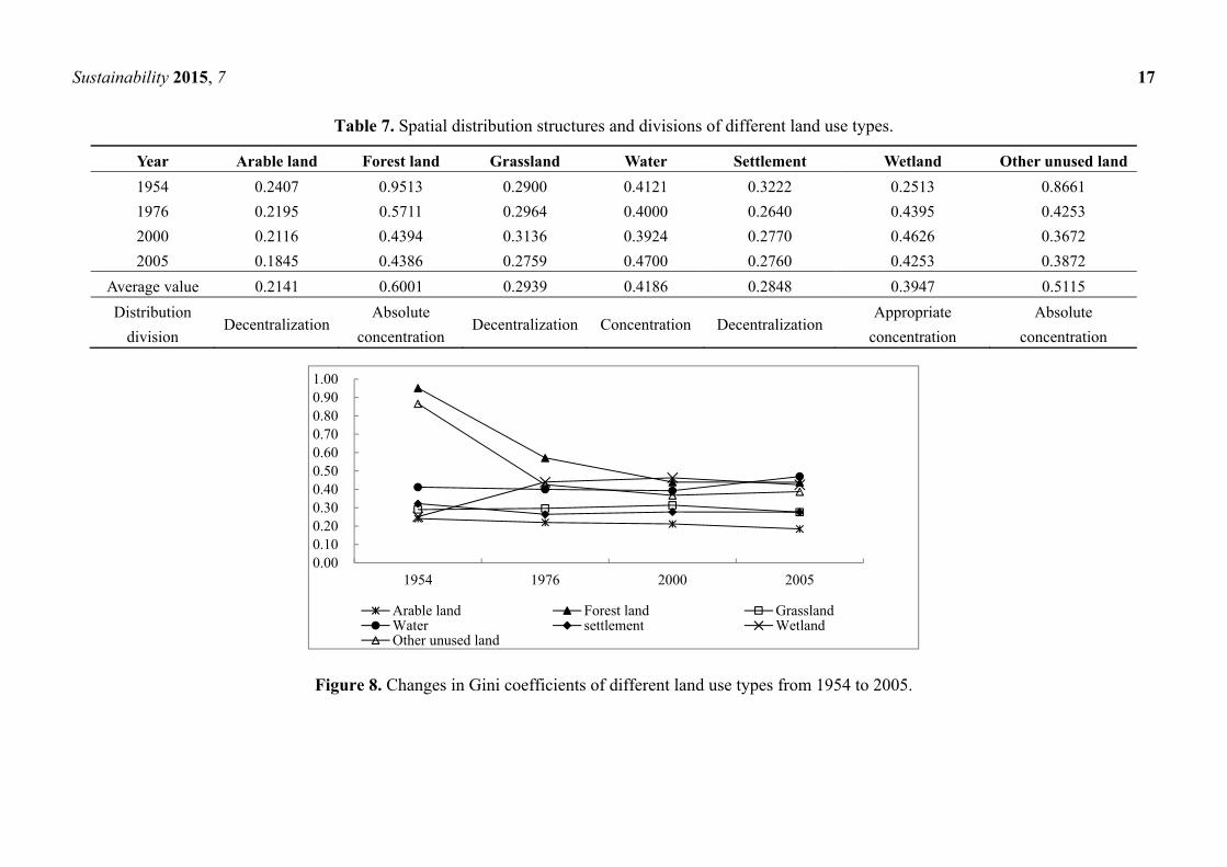
Figure 7 qualitatively demonstrates the respective distribution of land use structure between 1954 and
2005, while the Gini coefficient in the study area (Table 7 and Figure 8) quantitatively measures changes

Sustainability 2015, 7 16
of land use structure in the study period. From 1954 to 2005, there were great changes in the Gini
coefficients, especially those for forest land and other unused land. The average Gini coefficient of arable
land is 0.2141, the smallest among the Gini coefficients of the seven land use types. The results indicate
that during the study period, arable land was decentralized and had a trend of decentralized use explained
by the decreasing Gini coefficients over time. The average Gini coefficients of settlement and grassland
are 0.2848 and 0.2939, respectively, indicating that these two types of land use were distributed in
decentralized manners, with different change trends. Grassland had the minimal fluctuation. Water
bodies exhibited appropriate concentration, with an average Gini coefficient of 0.4186, and water bodies
tended toward concentration. Forest land had the highest average Gini coefficient at 0.6001, showing
absolute concentration. Other unused land had similar characteristics to forest land, and a decreasing
trend was clearly observable, especially from 1954 to 1976.
These changes in the Gini coefficients are consistent with the changes of the land use area. The area
of arable land and settlement increased during the study period, whereas their corresponding Gini
coefficients decreased and the spatial distributions were more even. Increases in cultivated land were
consistent with the result of population growth and excessive reclamation of land, which could be
reflected by increasing settlement. The growth of other unused land and the decrease of grassland and
wetland reflected the deterioration of the eco-environment [15,51] and therefore provided some evidence
indicating that the quality of the ecological environment declined year by year over the past decades.
Figure 7. Spatial Lorenz curves of various land use types.
0
20
40
60
80
100
0 20 40 60 80 100
Arable land
Forest land
Grassland
Water
Settlement
WetlandAcc
umul
ated
per
cent
age
of e
ach
land
-use
ty
pe (
%)
Accumulated percentage of land
1954yr
0
20
40
60
80
100
0 20 40 60 80 100
Arable land
Forest land
Grassland
Water
Settlement
Wetland
Accumulated percentage of land (%)
Acc
umul
ated
per
cent
age
of e
ach
land
-us
e ty
pe (
%)
1976 yr
0
20
40
60
80
100
0 20 40 60 80 100
Arable land
Forest land
Grassland
Water
Settlement
Wetland
Other unusedlandA
ccum
ulat
ed p
erce
ntag
e of
eac
hla
nd-u
se
type
(%
)
Accumulated percentage of land
2000 yr
0
20
40
60
80
100
0 20 40 60 80 100
Arable land
Forest land
Grassland
Water
Settlement
Wetland
Other unusedlandA
ccum
ulat
ed p
erce
ntag
e of
eac
hla
nd-u
se
type
(%
)
Accumulated percentage of land
2005 yr
Sustainability 2015, 7 17
Table 7. Spatial distribution structures and divisions of different land use types.
Year Arable land Forest land Grassland Water Settlement Wetland Other unused land
1954 0.2407 0.9513 0.2900 0.4121 0.3222 0.2513 0.8661
1976 0.2195 0.5711 0.2964 0.4000 0.2640 0.4395 0.4253
2000 0.2116 0.4394 0.3136 0.3924 0.2770 0.4626 0.3672
2005 0.1845 0.4386 0.2759 0.4700 0.2760 0.4253 0.3872
Average value 0.2141 0.6001 0.2939 0.4186 0.2848 0.3947 0.5115
Distribution
division Decentralization
Absolute
concentration Decentralization Concentration Decentralization
Appropriate
concentration
Absolute
concentration
Figure 8. Changes in Gini coefficients of different land use types from 1954 to 2005.
0.000.100.200.300.400.500.600.700.800.901.00
1954 1976 2000 2005
Arable land Forest land GrasslandWater settlement WetlandOther unused land

Sustainability 2015, 7 18
4. Conclusions
In this paper, we used published land cover data, based on topographic and environmental background
maps and also remotely sensed images including Landsat MSS and TM, to study the spatiotemporal
changes of land use and land cover from 1954 to 2005 in Zhenlai County, Jilin province, northeast China.
This study integrated methods of bitemporal change detection and temporal trajectory analysis to trace
the paths of land cover change for every location, and to identify the stability of land-use conversion and
human-induced environmental change. Spatial distribution structures of different land use types were
also analyzed by using the Lorenz curve and associated Gini coefficient. The findings of the case study
can be summarized as follows.
(1) The results of bitemporal change detection showed that land use/cover changed significantly in
Zhenlai County from 1954 to 2005. Arable land expanded at the expense of grassland and wetland.
Meanwhile, plenty of grassland was converted to other unused land, indicating serious
environmental degradation in Zhenlai County during the past decades.
(2) Trajectory analysis of land use and land cover change demonstrated that settlement, arable land, and
water bodies were relatively stable in terms of coverage and spatial distribution, while grassland,
wetland, and forest land had weak stability. Many transitions from wetland to other unused land
indicated that land degradation had difficult reversibility. Furthermore, human-induced changes,
representing an irreversible impact on the environment, could be distinguished from changes caused
by natural forces by using this trajectory analysis. The results suggested that natural forces were still
dominating the environmental processes of the study area, with unchanged (35.83% of the total
area) and indecisive changes between land-cover types (37.28%). However, human-induced
changes, constituting 26.89% of the total area, also played an important role in environmental change.
(3) The research showed that the Lorenz curve/Gini coefficient could be applied effectively to analyze
the land use structure changes. The seven types of land use displayed different concentration trends
and had large changes during 1954 and 2005. Arable land was the most decentralized, whereas forest
land was the most concentrated.
(4) Previous studies of spatiotemporal changes mainly focused on analyzing the categorical changes of
land cover with the accumulation of remotely sensed images using a bitemporal detection method.
It assumed spatially homogeneous transition rates and therefore was of limited use in projecting
future changes. The above results not only revealed notable spatiotemporal features of land
use/cover change in the time series, but also confirmed the applicability and effectiveness of the
combined methods of bitemporal change detection, temporal trajectory analysis, and a Lorenz
curve/Gini coefficient. Integrating methods of bitemporal change detection and temporal trajectory
analysis could explore the trajectories of land cover change by analyzing the extent to which land
use conversion is explained by the concept of stability and by distinguishing human-induced land
changes from natural evolution types, and then could effectively trace the paths of land cover change
for every location. Meanwhile, the Lorenz curve and Gini coefficient of economic models could
supplement and reveal the regularity in land use structural changes to gain a better understanding of
the human impact on this fragile ecosystem.

Sustainability 2015, 7 19
Acknowledgments
We thank the three reviewers for their constructive comments and suggestions. This research was
funded by the Strategic Priority Research Program of the Chinese Academy of Sciences (No.
XDA05090310), the National Natural Science Foundation of China (No. 41271416), and the State
Scholarship Fund of China. The paper was also completed with support from the Center for International
Earth Science Information Network (CIESIN), Columbia University, USA. We would like to thank
Robert S. Chen and Alex de Sherbinin of CIESIN for their valuable suggestions.
Author Contributions
Yuanyuan Yang and Shuwen Zhang conceived and designed the research; Shuwen Zhang and Jiuchun
Yang collected and processed the data; Yuanyuan Yang, Dongyan Wang and Xiaoshi Xing analyzed the
data. All authors have read and approved the final manuscript.
Conflicts of Interest
The authors declare no conflict of interest.
References
1. Lambin, E.F. Modelling and monitoring land-cover change processes in tropical regions. Prog.
Phys. Geogr. 1997, 21, 375–393.
2. Turner, B.L.; Lambin, E.F.; Reenberg, A. The emergence of land change science for global
environmental change and sustainability. Proc. Natl. Acad. Sci. USA 2007, 104, 20666–20671.
3. Foster, D.; Swanson, F.; Aber, J.; Burke, I.; Brokaw, N.; Tilman, D.; Knapp, A. The importance of
land-use legacies to ecology and conservation. Bioscience 2003, 53, 77–88.
4. Gragson, T.L.; Bolstad, P.V. Land use legacies and the future of southern Appalachia. Soc. Nat.
Resour. 2006, 19, 175–190.
5. Lambin, E.F.; Turner, B.L.; Geist, H.J.; Agbola, S.B.; Angelsen, A.; Bruce, J.W.; Coomesf, O.T.;
Dirzog, R.; Fischerh, G.; Folkei, C.; et al. The causes of land-use and land-cover change: Moving
beyond the myths. Glob. Environ. Chang. 2001, 11, 261–269.
6. Chauchard, S.; Carcaillet, C.; Guibal, F. Patterns of land-use abandonment control tree-recruitment
and forest dynamics in Mediterranean mountains. Ecosystems 2007, 10, 936–948.
7. DeFries, R.S.; Eshleman, K.N. Land-use change and hydrologic processes: A major focus for the
future. Hydrol. Process. 2004, 18, 2183–2186.
8. Costanza, R.; d’Arge, R.; de Groot, R.; Farber, S.; Grasso, M.; Hannon, B.; Limburg, K.; Naeem, S.;
O’Nelll, R.V.; Paruelo, J.; et al. The value of the world’s ecosystem service and natural capital.
Nature 1997, 387, 253–260.
9. Chen, Y.H.; Li, X.B.; Su, W.; Li, Y. Simulating the optimal land-use pattern in the farming-pastoral
transitional zone of Northern China. Computers. Environ. Urban Syst. 2008, 32, 407–414.
10. Wang, J.A.; Xu, X.; Liu, P.F. Land use and carrying capacity in ecotone between agriculture and
animal husbandry in northern China. Resour. Sci. 1999, 21, 19–24. (In Chinese)

Sustainability 2015, 7 20
11. Lin, N.; Tang, J.; Bian, J.M.; Yang, J.Q. The quaternary environmental evolution and the problem
of desertification in northeast plain. Quat. Sci. 1999, 5, 448–455.
12. Ren, C.Y.; Zhang, B.; Wang, Z.M.; Song, K.S.; Liu, D.W.; Liu, Z.M. A GIS-based Tupu analysis
of dynamics of saline-alkali land in western Jilin province. Chin. Geogr. Sci. 2007, 17, 333–340.
13. Wang, Z.Q.; Zhang, B.; Yu, L.; Zhang, S.Q.; Wang, Z.M. Study on LUCC and the ecological security
response of wetlands in western Jilin province. Arid Zone Res. 2004, 21, 97–103. (In Chinese)
14. Zang, L.J.; Jiang, Q.G.; Wang, F.Y. Adjustment of land utilization structure in Zhenlai County.
Glob. Geol. 2010, 29, 149–154. (In Chinese)
15. Tang, J.; Wang, X.G. Analysis of the land use structure changes based on Lorenz curves. Environ.
Monit. Assess. 2009, 151, 175–180.
16. Wang, Z.Q.; Zhang, B.; Zhang, S.Q.; Wang, Z.M. Study on dynamics of landscape and responses
of ecological security to it in west Jilin province. J. Soil Water Conserv. 2005, 19, 131–136.
(In Chinese)
17. Rogan, J.; Chen, D.M. Remote sensing technology for mapping and monitoring land-cover and
land-use change. Progr. Plan. 2004, 61, 301–325.
18. Xiao, H.L.; Weng, Q.H. The impact of land use and land cover changes on land surface temperature
in a karst area of China. J. Environ. Manag. 2007, 85, 245–257.
19. Coppin, P.; Jonckheere, I.; Nackaerts, K.; Muys, B.; Lambin, E. Digital change detection methods
in ecosystem monitoring: A review. Int. J. Remote Sens. 2004, 25, 1565–1596.
20. Shafizadeh Moghadam, H.; Helbich, M. Spatiotemporal urbanization processes in the megacity of
Mumbai, India: A Markov chains-cellular automata urban growth model. Appl. Geogr. 2013, 40,
140–149.
21. Deng, J.S.; Wang, K.; Li, J.; Deng, Y.H. Urban land use change detection using multisensory
satellite images. Pedosphere 2009, 19, 96–103.
22. Weber, C.; Petropoulou, C.; Hirsch, J. Urban development in the Athens metropolitan area using
remote sensing data with supervised analysis and GIS. Int. J. Remote Sens. 2005, 26, 785–796.
23. Deng, J.S.; Wang, K.; Hong, Y.; Qi, J.G. Spatio-temporal dynamics and evolution of land use change
and landscape pattern in response to rapid urbanization. Landsc. Urban Plan. 2009, 92, 187–198.
24. Long, H.L.; Wu, X.Q.; Wang, W.J.; Dong, G.H. Analysis of urban-rural land-use change during
1995–2006 and its policy dimensional driving forces in Chongqing, China. Sensors 2008, 8, 681–699.
25. Dewan, A.M.; Yamaguchi, Y.; Rahman, M.Z. Dynamics of land use/cover changes and the analysis
of landscape fragmentation in Dhaka Metropolitan, Bangladesh. GeoJournal 2012, 77, 315–330.
26. Buyantuyev, A.; Wu, J.G.; Gries, C. Multiscale analysis of the urbanization pattern of the Phoenix
metropolitan landscape of USA: Time, space and thematic resolution. Landsc. Urban Plan. 2010,
94, 206–217.
27. Zhou, Q.M.; Li, B.L.; Kurban, A. Trajectory analysis of land cover change in arid environment of
China. Int. J. Remote Sens. 2008, 29, 1093–1107.
28. Wang, D.C.; Gong, J.H.; Chen, L.D.; Zhang, L.H.; Song, Y.Q.; Yue, Y.J. Comparative analysis of
land use/cover change trajectories and their driving forces in two small watersheds in the western
Loess Plateau of China. Int. J. Appl. Earth Obs. Geoinf. 2013, 21, 241–252.
29. Mertens, B.; Lambin, E.F. Land-cover-change trajectories in southern Cameroon. Ann. Assoc. Am.
Geogr. 2000, 90, 467–494.
Sustainability 2015, 7 21
30. Wang, D.C.; Gong, J.H.; Chen, L.D.; Zhang, L.H.; Song, Y.Q.; Yue, Y.J. Spatio-temporal pattern
analysis of land use/cover change trajectories in Xihe watershed. Int. J. Appl. Earth Obs. Geoinf.
2012, 14, 12–21.
31. Zhou, Q.M.; Li, B.L.; Kurban, A. Spatial pattern analysis of land cover change trajectories in
Tarim Basin, northwest China. Int. J. Remote Sens. 2008, 29, 5495–5509.
32. Swetnam, R.D. Rural land use in England and Wales between 1930 and 1998: Mapping trajectories
of change with a high resolution spatio-temporal dataset. Landsc. Urban Plan. 2007, 81, 91–103.
33. Bai, S.Y.; Zhang, S.W. A study on the spatial-temporal land use conversion in county region–Taking
Duerbete county as an example. J. Arid Land Resour. Environ. 2005, 19, 67–70. (In Chinese)
34. Zhao, B.; Kreuter, U.; Li, B.; Ma, Z.J.; Chen, J.K.; Nakagoshi, N. An ecosystem service value
assessment of land-use change on Chongming Island, China. Land Use Policy 2004, 21, 139–148.
35. Isong, M.; Eyo, E.; Eyoh, A.; Nwanekezie, O.; Olayinka, D.N.; Udoudo, D.O.; Ofem, B. GIS
cellular automata using artificial neural network for land use change simulation of Lagos, Nigeria.
J. Geogr. Geol. 2012, 4, 94–101.
36. Lin, Y.P.; Chu, H.J.; Wu, C.F.; Verburg, P.H. Predictive ability of logistic regression, auto-logistic
regression and neural network models in empirical land-use change modeling—A case study. Int.
J. Geogr. Inf. Sci. 2011, 25, 65–87.
37. Lin, Z.M.; Xia, B.; Dong, W.J. Analysis on temporal-spatial changes of land-use structure in
Guangdong province based on information entropy. Trop. Geogr. 2011, 31, 266–271. (In Chinese)
38. Henseler, M.; Wirsig, A.; Herrmann, S.; Krimly, T.; Dabbert, S. Modeling the impact of global
change on regional agricultural land use through an activity-based non-linear programming
approach. Agric. Syst. 2009, 100, 31–42.
39. Huang, Y.; Xia, B.; Yang, L. Relationship study on land use spatial distribution structure and
energy-related carbon emission intensity in different land use types of Guangdong, China,
1996–2008. Sci. World J. 2013, 2013, Article ID 309680.
40. Zheng, X.Q.; Xia, T.; Yang, X.; Yuan, T.; Hu, Y.C. The land Gini coefficient and its application
for land use structure analysis in China. PLoS One 2013, 8, e76165.
41. Ramankutty, N.; Foley, J.A. Estimating historical changes in global land cover: Croplands from
1700 to 1992. Glob. Biogeochem. Cycles 1999, 13, 997–1027.
42. Petit, C.C.; Lambin, E.F. Long-term land-cover changes in the Belgian Ardennes (1775–1929):
Model-based reconstruction vs. Historical maps. Glob. Chang. Biol. 2002, 8, 616–630.
43. Local Record of Zhenlai County; Jilin People’s Press: Changchun, China, 1995. (In Chinese)
44. Bai, S.Y.; Zhang, S.W. The discussion of the method of land utilization spatial information
reappearance of history period. J. Arid Land Resour. Environ. 2004, 18, 77–80. (In Chinese)
45. Bai, S.Y.; Zhang, S.W.; Zhang, Y.Z. Study on the method of diagnose the plowland spacial
distribution in historical era. Syst. Sci. Comp. Stud. Agric. 2005, 21, 252–255. (In Chinese)
46. Liu, J.Y.; Liu, M.L.; Zhuang, D.F.; Zhang, Z.X.; Deng, X.Z. Study on spatial pattern of land-use
change in China during 1995–2000. Science China 2003, 46, 374–384.
47. Bai, S.Y.; Zhang, S.W.; Zhang, Y.Z. Stages and determinants of farmland development and driving
forces in Duerbote County during the past 50 years. Resour. Sci. 2005, 27, 71–76. (In Chinese)
48. Lu, X.N.; Deng, W.; Zhang, S.Q.; Xong, D.H.; Xin, X. Land-use changes along the lower reaches
of Huolin river in the last 50 years. J. Arid Land Resour. Environ. 2007, 21, 68–74. (In Chinese)

Sustainability 2015, 7 22
49. Liu, X.N.; Huang, F. Analysis of the regional co-environmental effect driving by LUCC.
J. Northeast Norm. Univ. 2002, 34, 87–92. (In Chinese)
50. Song, K.S.; Liu, D.W.; Wang, Z.M.; Zhang, B.; Jin, C.; Li, F.; Liu, H.J. Land use change in Saijiang
plain and its driving forces analysis since 1954. Acta Geogr. Sinica 2008, 63, 93–104. (In Chinese)
51. Wang, X.G.; Tang, J.; Li, Z.Y.; Wang, C.Y. Analysis of land use structure change in western of
Jilin province based on Lorrenze curves. Res. Agric. Mod. 2007, 28, 310–313. (In Chinese)
© 2014 by the authors; licensee MDPI, Basel, Switzerland. This article is an open access article
distributed under the terms and conditions of the Creative Commons Attribution license
(http://creativecommons.org/licenses/by/4.0/).