Spatio-temporal variation in pike Spatio-temporal variation in pike demography and dispersal: demography and dispersal:

effects of harvest intensity and effects of harvest intensity and population densitypopulation density

Thrond O Haugen

Who’s involved?Who’s involved?

Project leader: Nils Chr. Stenseth Centre for Ecology and Hydrology

• Ian Winfield University of Oslo

• Leif Asbjørn Vøllestad• Per Aass (Zoologisk museum)

Management• Tore Qvenild (Hedmark)• Ola Hegge (Oppland)• NIVA

• Gösta Kjellberg

Size-biased harvest of fishSize-biased harvest of fish

Ecological implications• Affects demography directly

• Effects on population dynamics

• Affects population density that in turn will affect growth conditions

Evolutionary implications• Life-history adaptations to man-made

mortality regime and growth conditions

General project objectivesGeneral project objectives In order to gain better knowledge

of pike population dynamics:• Estimate demographic rates under

changing harvesting regimes• Quantify natural- and fishing mortality• Estimate recruitment to fisheries• Estimate dispersal under varying

population densities

Over to England...Over to England...

Data backgroundData background Tagged during spring

• Three methods• Pike gill nets (64 mm

mesh size)• 46 mm gill nets• Perch traps

• Live recaptures (all re-released)

Winter fisheries by scientists only (64 mm)• All individuals retrieved

1949–present

Leng

th

20

30

40

50

60

70

80

90

100

110

GN PGN PT

Method

Perch trap (PT) – for tagging

64 mm gillnet (PGN) – retrieved

46/64 mm gillnet (GN) – for tagging

M A M J J A S O N DFJ M AFJ M

pGN(t)pPT(t)

pGN(t+2)pPT(t+2)

pPGN(t+1)

Right-censoring

(t) (t+1)

7 months 5 months

Discretizing the dataDiscretizing the data

p (t) p (t+2)

Changed fishing effortChanged fishing effort

100

1000

10000

1945 1955 1965 1975 1985 1995 2005

Net

ting

eff

ort

(30

yd n

et d

ays) North

South

Total

DDensity-dependent growth, ensity-dependent growth, but what about survival?but what about survival?

r P = -0.77

r P = -0.69

r P = -0.47

500

550

600

650

700

750

800

850

0 1000 2000 3000 4000 5000

Estimated population size

Size

(cm

)

1 2 3 4 5 1 2 3 4 5

Age40 50 60 70 80 90 100 1100

100

200

300

400

500

Nu

mb

er

of

ind

ivid

ua

ls

Length (cm)

64 mm gill net

Kipling (1983), J. Anim. Ecol.

Specific objectivesSpecific objectives We have exact measures on fishing

effort• Is fishing mortality related to effort?

• If so: does this apply to all size classes in both basins?

We have population size estimates and information about individual growth• Is natural survival density dependent?• Is dispersal density dependent?

• If so: does this apply to all size classes in both basins?

Multistate modelsMultistate models

Probability of survival-migration

State 1, 2 or 3i (1,1) i (1,2) i (1,3)

i (2,1) i (2,2) i (2,3)

i (3,1) i (3,2) i (3,3)

Capture probability

State 1State 2State 3

pi+1 (1,1) pi+1 (1,2) pi+1 (1,3)

pi+1 (1) pi+1 (2) pi+1

(3)or

From

To

Jolly MoVe-parameterisation (JMV)

Conditional Arnason-Schwartz parameterisation (CAS)

The transition parameterThe transition parameter

May estimate a separate transition parameter () when conditioning on survival• i,j = i,j/Si

S = fidelity-survivali = from-statej = to-state

Note: S is estimated for the “from” state and p for the “to” state in CAS parameterisation

ParameterisationParameterisation

A: NSN…B: S0N…

N3

SN2

S2

S2

NS1

N1 pSpS Pr(A):

N3

SN2

S2

S2

SS1

NN2

N2

N2

SN1

S1 )( pSqSqS

ik

ik pq 1

Pr(B):

moves

stays

GOF tests for CJS modelsGOF tests for CJS models

A fully efficient GOF test for the CJS model is based on the property that all animals present at any given time behave the same• whatever their past capture history

(Test 3)• whether they are currently captured

or not (Test 2)

NOW: GOF tests also for MS NOW: GOF tests also for MS modelsmodels

A fully efficient GOF test for the JMV model is based on the property that all animals present at any given time on the same site behave the same• whatever their past capture history (Test 3G)• whether they are currently captured or not

(Test M)

Methods described in Pradel et al. 2003, Biometrics• U-Care 2.0 (ftp://ftp.cefe.cnrs-mop.fr/biom/Soft-CR/)

Model constraints (I)Model constraints (I)

Because of right censoring at winter occasions neither S or is separatetly estimable for winter-to-spring intervals• Could set S=1 and = 0 for these

periods or force estimates to equal over both periods within a year• Last approach more often converged

Model constraints (II)Model constraints (II) p could be estimated for each

occasion• Three different methods used during

spring• Different efforts and size selectivity• time models the only possibility

• Same gillnets used during winter fisheries throughout the study• Could constrain according to effort• Could estimate size-dependent recruitment

to fisheries

• p-estimates performed under maximum temporal variation for S and

Analysis outlineAnalysis outline

1. Analysis of natural survival• Using spring records only• Standard CJS modelling• Collapsing basin information• Exploring effects from gear and

density

2. MS modelling• Including winter captures (fishing

mortality)• Recruitment to fisheries

• Between-basin dispersal

GOFs for CJSGOFs for CJS For the 1953-1986 period No evidence for lack of fit for the CJS

model• No trap happiness or shynessTest type 2 p df

Test 3.SR 21.7 0.65 25

Test 3.SM 9.23 0.98 20

Test 2.CT 25.7 0.43 25

Test 2.CL 12.4 0.83 18

Global 68.8 0.94 88

Length- and gear-specific Length- and gear-specific recapture probabilityrecapture probability

0

0.1

0.2

0.3

0.4

0.5

0.6

0 20 40 60 80 100

Tagging length (cm)

Ca

ptu

re p

rob

ab

ility

Perch trap

Gill nets

pa1(gear*length+length2

), a>1(t)

Temporal variation in annual Temporal variation in annual natural survivalnatural survival

0.0

0.1

0.2

0.3

0.4

0.5

0.6

0.7

0.8

0.9

1.053

-54

54-5

555

-56

56-5

757

-58

58-5

959

-60

60-6

161

-62

62-6

363

-64

64-6

565

-66

66-6

767

-68

68-6

969

-70

70-7

171

-72

72-7

373

-74

74-7

575

-76

76-7

777

-78

78-7

979

-80

An

nu

al s

urv

iva

l pro

ba

bili

ty

Perch trap and seine

Gill nets

(gear+t)

perch disease

Fishing effort and natural Fishing effort and natural survivalsurvival

0

0.1

0.2

0.3

0.4

0.5

0.6

0 500 1000 1500 2000 2500 3000 3500 4000

Pike gill net effort (30 yd net days)

Ann

ual n

atur

al s

urvi

val r

ate

Perch trap

Gill nets

(gear+effortPGN)

Summary of the CJS Summary of the CJS resultsresults

Natural survival vary over time• decreased during 1960-1980 period• indication of density dependence?

Capture probability is gear and size specific• As known…

Do MS-CMR models fit the Do MS-CMR models fit the data?data?

Test type 2 p df

Test 3G 23.471 0.987 41

Test M 49.885 0.002 21

GOF J MV 72.277 0.175 62

GOF CAS 104.838 0.000 33

41ˆ2

df

c

Occasion 2 p

2 0.000 1.000 3 0.000 1.000 4 1.101 0.294 5 0.234 0.632 6 0.244 0.622 7 0.242 0.623 8 0.011 0.916 9 0.816 0.366

10 25.000 0.000 11 2.112 0.146 12 0.844 0.330 13 5.500 0.019 14 1.546 0.214 15 0.058 0.809 16 0.152 0.696 17 3.643 0.056 18 1.172 0.279 19 0.563 0.453 20 0.175 0.676 21 0.686 0.408 22 0.750 0.386 23 4.286 0.038 24 0.000 1.000 25 0.000 1.000 26 0.750 0.386

Sum 49.885 0.002

Sum-occ10 24.885 0.412

Final CAS modelFinal CAS model

Sa1(basin*length),Sa>1(basin*popsize)

Pspring(basin+t), PSwinter,a1(length), PN

winter,a1(.), Pwinter,a>1(basin+effort)

NSa1(length), NS

a>1(density gradient), SN (t)

Size-dependent recruitment Size-dependent recruitment to PGN fisheriesto PGN fisheries

0.00

0.05

0.10

0.15

0.20

0.25

0.30

0.35

0.0 20.0 40.0 60.0 80.0 100.0

length at tagging, L(t)

pro

ba

bili

ty o

f PG

N c

ap

ture

at t

+1

Effort and fishing mortalityEffort and fishing mortality

0.00

0.05

0.10

0.15

0.20

0.25

-4.0 -2.0 0.0 2.0 4.0

scaled effort (SD)

pro

ba

bili

ty o

f PG

N c

ap

ture

for

a>

1

Northern

Southern

Basin- and year-specific Basin- and year-specific survivalsurvival

0.0

0.1

0.2

0.3

0.4

0.5

0.6

0.7

0.8

0.9

1.019

53

1954

1955

1956

1957

1958

1959

1960

1961

1962

1963

1964

1965

1966

1967

1968

1969

1970

1971

1972

1973

1974

1975

1976

1977

1978

1979

1980

-199

0

half-

year

sur

viva

l pro

babi

lity

N

S

Length-dependent survival Length-dependent survival from tagging to first winterfrom tagging to first winter

0.00.10.20.30.40.50.60.70.80.91.0

0 20 40 60 80 100

Length at tagging (cm)

prob

of

surv

ival

ove

r a1

Northern Southern

Sa1(basin*length)

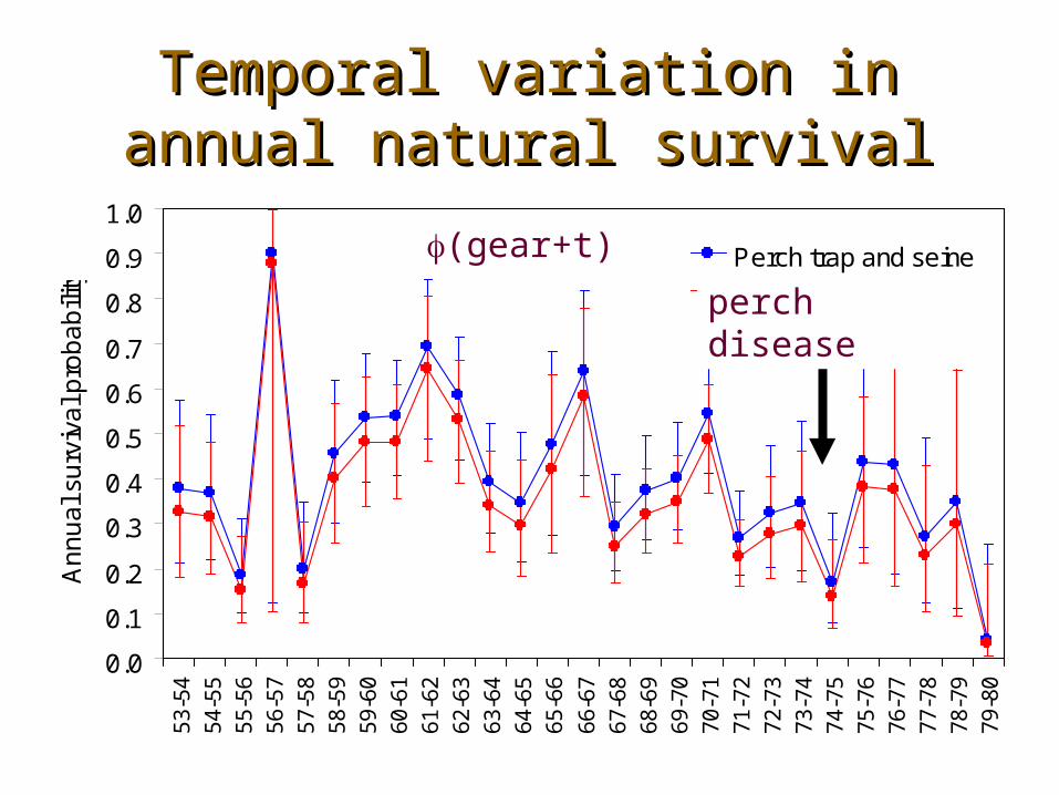
0.70

0.75

0.80

0.85

0.90

0 500 1000 1500 2000 2500 3000

Population size

half

-yea

r su

rviv

al p

roba

bility

Northern

Southern

Density-dependent survival Density-dependent survival for tagging age>1for tagging age>1

Sa>1(basin*popsize)

Size- and basin-dependent Size- and basin-dependent dispersal during first year dispersal during first year

following taggingfollowing tagging

0.00

0.05

0.10

0.15

0.20

0.25

0.30

0.35

0.40

0 20 40 60 80 100

Length at tagging (cm), L(t)

prob

of

N->

S du

ring

t t

o t+

2

0

0.1

0.2

0.3

0.4

0.5

0.6

0.7

0.8

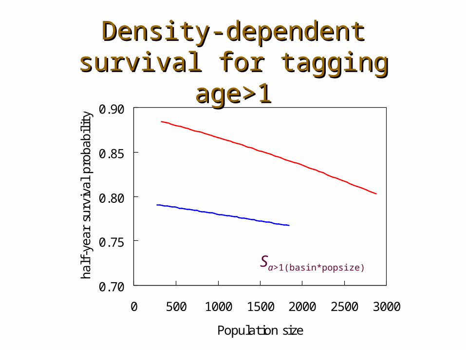
-1.5 -1.0 -0.5 0.0 0.5 1.0 1.5 2.0

relativ density gradient

pro

ba

bili

ty o

f mig

ratio

n d

uri

ng

six

mo

nth

s

N->S

S->N

Density- and basin-Density- and basin-dependent dispersal for a>1dependent dispersal for a>1

Increasing relative density in north

SummarySummary Indications of density-dependent

dispersal and survival• Basin specific responses

Net migration from N to S• larger ones migrate with higher probability

3-4 times higher fishing mortality in S Once lengths of >55 cm is achieved

fishing mortality increase with effort Possible to predict recruitment to

fisheries from spring length distributions• not for N

Further objectives to be Further objectives to be addressedaddressed

Effect of sex Population composition

• Age/size structure Effects from other environmental

variables• Eutrophication• Prey abundance, i.e. perch abundance• Temperature

Should I stay or should I

go?

)29.179.0(

)29.179.0(

1)SNPr(

e

e