Embed Size (px)
Citation preview
Spatio-Temporal Join Selectivity
Jimeng Sun
Department of Computer Science Carnegie Mellon University
Pittsburgh, PA, USA [email protected]
Yufei Tao
Department of Computer Science City University of Hong Kong Tat Chee Avenue, Hong Kong
Dimitris Papadias
Department of Computer Science Hong Kong University of Science and Technology
Clear Water Bay, Hong Kong [email protected]
George Kollios
Department of Computer Science Boston University Boston, MA, USA [email protected]
Abstract
Given two sets S1, S2 of moving objects, a future timestamp tq, and a distance threshold d, a
spatio-temporal join retrieves all pairs of objects that are within distance d at tq. The selectivity
of a join equals the number of retrieved pairs divided by the cardinality of the Cartesian product
S1×S2. This paper develops a model for spatio-temporal join selectivity estimation based on
rigorous probabilistic analysis, and reveals the factors that affect the selectivity. Initially, we
solve the problem for 1D (point and rectangle) objects whose location and velocities distribute
uniformly, and then extend the results to multi-dimensional spaces. Finally, we deal with non-
uniform distributions using a specialized spatio-temporal histogram. Extensive experiments
confirm that the proposed formulae are highly accurate (average error below 10%).
Information Systems, 31(8), 793-813, 2006.
Recommended by Yannis Ioannidis, Area Editor.
Contact Author: Dimitris Papadias Department of Computer Science Hong Kong University of Science and Technology Clear Water Bay, Hong Kong Office: ++852-23586971 http://www.cs.ust.hk/~dimitris/ Fax: ++852-23581477 E-mail: [email protected]
This is the Pre-Published Version

2
1. INTRODUCTION
An important operation in spatio-temporal databases and mobile computing systems is to predict objects’
future location based on information at the current time (e.g., for collision detection). For this purpose the
database usually represents object movement as a function of time and stores the function parameters [14,
1, 24, 23]. As an example, given the location o(0) of object o at the current time 0 and its velocity oV, its
position at future time t can be computed as o(t)=o(0)+oV ·t. According to this representation, an update is
necessary only when the function parameters (i.e., oV) change.
Given two sets S1, S2 of objects, a spatio-temporal join retrieves all pairs of objects <o1, o2> such that
o1∈S1, o2∈S2, and |o1(tq), o2(tq)|≤d, i.e., the distance |o1(tq), o2(tq)| between objects o1 and o2 at a (future)
query timestamp tq is below a threshold d. For instance, consider the query “retrieve all pairs of airplanes
that will come closer than 10 miles 5 minutes from now”. This (self-join) example outputs pairs of
moving objects; in some cases one of the inputs can be static: “retrieve all pairs <city c, typhoon t> such
that t will cover c at 9am tomorrow according to the current spreading speed of t”. An important variation
is the constrained join, which involves an additional constraint window to limit the data space of interest.
For instance, in the previous example, an analyst may be interested only in cities in the southeast US
region.
In this paper we discuss the selectivity of spatio-temporal joins, which is defined as the number of
result pairs divided by the size of the cartesian product of the input datasets. Estimating the join
selectivity is important for several reasons.
• As with conventional and spatial [16] databases, selectivity estimation is vital to query optimization
for computing the best execution plan.
• In many applications users are interested in the number of joined pairs (i.e., a join counting query)
rather than the concrete results. For example, prediction of potential congestions requires the traffic
volume rather than the ids of cars [21]. Furthermore, stream (spatio-temporal) databases [11, 8] may
maintain only aggregate information in order to deal with voluminous updates.
• Performing an exact join (which is time consuming) is meaningless in applications with very frequent
motion function changes because the result may already be invalidated before the join processing
terminates. In such cases, a fast estimation of the output size is the only meaningful computation that
can be performed given the tight time limit.
Although spatial join selectivity can be computed using several methods [4, 9, 22], their application in
spatio-temporal scenarios leads to significant error. Similarly, existing work [7] on estimation of spatio-
temporal window queries on a single dataset cannot be efficiently adapted for joins. Motivated by this, we

3
address the problem by first proposing fundamental probabilistic formulae for spatio-temporal joins on
uniform (point and rectangular) objects. Then, we integrate these equations with spatio-temporal
histograms to support non-uniform data. Compared to the previous approaches, the proposed histogram
achieves significantly lower estimation error and is incrementally updatable (whereas previous solutions
require frequent re-construction). We evaluate the efficiency of our methods with extensive
experimentation.
The rest of the paper is organized as follows. Section 2 reviews previous work on spatial joins,
histograms, and spatio-temporal prediction. Section 3 analyzes spatio-temporal join selectivity on uniform
data, while Section 4 extends the results to non-uniform data (using histograms). Section 5 experimentally
evaluates the proposed methods, and Section 6 concludes the paper with directions for future work.
2. RELATED WORK
Section 2.1 overviews spatial join algorithms (assuming knowledge of R-trees [10, 6]), and join
selectivity estimation on static objects. Section 2.2 introduces MinSkew, a multi-dimensional histogram
that constitutes the starting point of our spatio-temporal histogram. Section 2.3 discusses spatio-temporal
range selectivity and elaborates why it cannot be applied for join selectivity estimation. Finally Section
2.4 reviews the Time Parameterized R-tree (TPR-tree), an index structure for moving objects which is
employed in our histogram techniques.
2.1 Spatial Join Selectivity
Consider two objects o1, o2 belonging to spatial datasets S1, S2 and satisfying the join condition |o1, o2|≤d.
Join processing algorithms [5, 12, 15] are based on the observation that o1 and o2 should reside in R-tree
nodes E1 and E2 respectively, whose minimum bounding rectangles (MBRs) satisfy the property |E1,
E2|≤d. Thus, qualifying pairs are retrieved by synchronously traversing the R-trees of S1 and S2 in a top-
down fashion, recursively following node pairs that are within the distance constraint. The special case
where d=0 corresponds to the intersection join and has received considerable attention. Notice, however,
that intersection join is not meaningful for point data since it reduces to equality of points.
Spatial join selectivity was first studied in [3], which presents a formula for uniform data using the
results of previous work [13, 20] on window query selectivity. Several histogram-based approaches have
been proposed for non-uniform distributions. In particular, the histograms of [27, 16] divide the universe
regularly, while more sophisticated techniques [4, 22] perform the partitioning according to the data
distribution. On the other hand [9] employs a different approach based on power laws. Further, [16]
studies the selectivity of complex queries that involve multiple datasets. All the above methods require
the knowledge of distributions of the join datasets. In spatio-temporal databases, however, the distribution
4
continuously changes due to object movements. Hence, it is extremely expensive (both in terms of
computation time and storage cost) to pre-compute the distributions for future timestamps. Furthermore,
even if such distributions are obtained, they will soon be invalidated due to subsequent updates, rendering
re-computation necessary. Therefore, traditional approaches for spatial join selectivity are insufficient for
moving objects. Effective techniques should take the specialized problem characteristics into account.
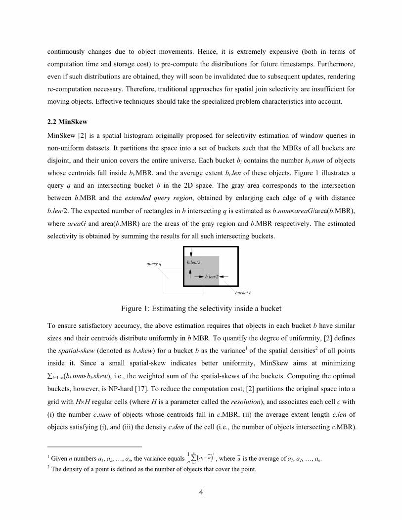
2.2 MinSkew
MinSkew [2] is a spatial histogram originally proposed for selectivity estimation of window queries in
non-uniform datasets. It partitions the space into a set of buckets such that the MBRs of all buckets are
disjoint, and their union covers the entire universe. Each bucket bi contains the number bi.num of objects
whose centroids fall inside bi.MBR, and the average extent bi.len of these objects. Figure 1 illustrates a
query q and an intersecting bucket b in the 2D space. The gray area corresponds to the intersection
between b.MBR and the extended query region, obtained by enlarging each edge of q with distance
b.len/2. The expected number of rectangles in b intersecting q is estimated as b.num×areaG/area(b.MBR),
where areaG and area(b.MBR) are the areas of the gray region and b.MBR respectively. The estimated
selectivity is obtained by summing the results for all such intersecting buckets.
bucket b
b.len/2
b.len/2
query q
Figure 1: Estimating the selectivity inside a bucket
To ensure satisfactory accuracy, the above estimation requires that objects in each bucket b have similar
sizes and their centroids distribute uniformly in b.MBR. To quantify the degree of uniformity, [2] defines
the spatial-skew (denoted as b.skew) for a bucket b as the variance1 of the spatial densities2 of all points
inside it. Since a small spatial-skew indicates better uniformity, MinSkew aims at minimizing
∑i=1~n(bi.num⋅bi.skew), i.e., the weighted sum of the spatial-skews of the buckets. Computing the optimal
buckets, however, is NP-hard [17]. To reduce the computation cost, [2] partitions the original space into a
grid with H×H regular cells (where H is a parameter called the resolution), and associates each cell c with
(i) the number c.num of objects whose centroids fall in c.MBR, (ii) the average extent length c.len of
objects satisfying (i), and (iii) the density c.den of the cell (i.e., the number of objects intersecting c.MBR).
1 Given n numbers a1, a2, …, an, the variance equals ( )2
1
1 n
ii
a an =
−∑ , where a is the average of a1, a2, …, an. 2 The density of a point is defined as the number of objects that cover the point.
5
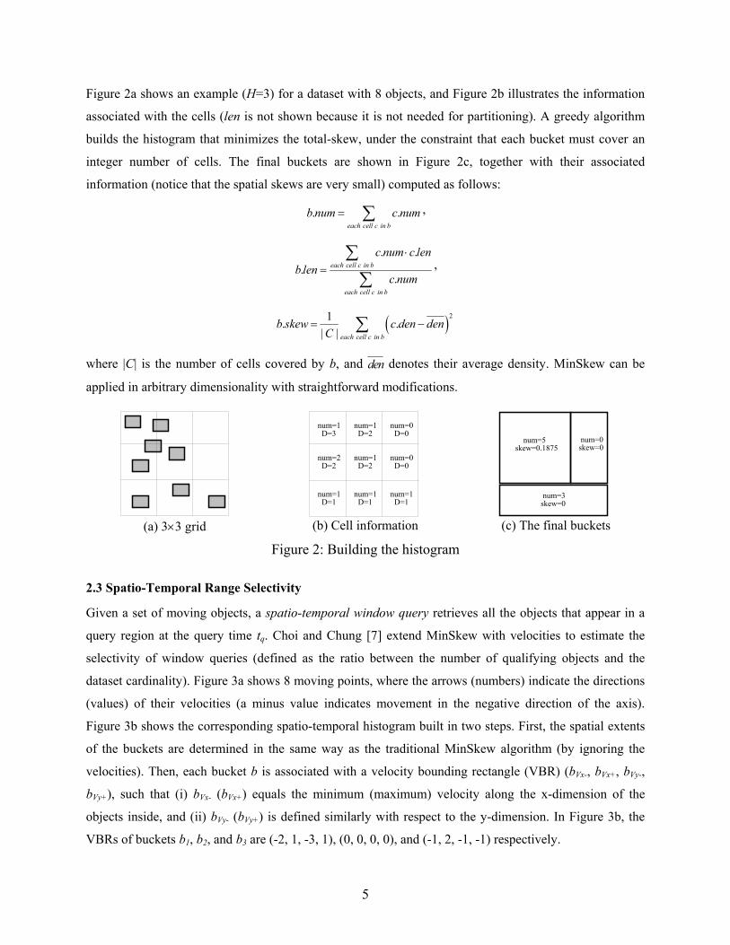
Figure 2a shows an example (H=3) for a dataset with 8 objects, and Figure 2b illustrates the information
associated with the cells (len is not shown because it is not needed for partitioning). A greedy algorithm
builds the histogram that minimizes the total-skew, under the constraint that each bucket must cover an
integer number of cells. The final buckets are shown in Figure 2c, together with their associated
information (notice that the spatial skews are very small) computed as follows:
. .each cell c in b
b num c num= ∑ ,
. .
..
each cell c in b
each cell c in b
c num c len
b lenc num
⋅=
∑∑
,
( )2
1. .
| | each cell c in b
b skew c den denC
= −∑
where |C| is the number of cells covered by b, and den denotes their average density. MinSkew can be
applied in arbitrary dimensionality with straightforward modifications.
num=1D=3
num=1D=2
num=0D=0
num=0D=0
num=2D=2
num=1D=2
num=1D=1
num=1D=1
num=1D=1
num=5skew=0.1875
num=0skew=0
num=3skew=0
(a) 3×3 grid (b) Cell information (c) The final buckets
Figure 2: Building the histogram
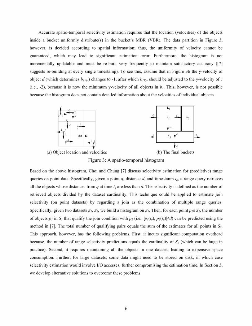
2.3 Spatio-Temporal Range Selectivity
Given a set of moving objects, a spatio-temporal window query retrieves all the objects that appear in a
query region at the query time tq. Choi and Chung [7] extend MinSkew with velocities to estimate the
selectivity of window queries (defined as the ratio between the number of qualifying objects and the
dataset cardinality). Figure 3a shows 8 moving points, where the arrows (numbers) indicate the directions
(values) of their velocities (a minus value indicates movement in the negative direction of the axis).
Figure 3b shows the corresponding spatio-temporal histogram built in two steps. First, the spatial extents
of the buckets are determined in the same way as the traditional MinSkew algorithm (by ignoring the
velocities). Then, each bucket b is associated with a velocity bounding rectangle (VBR) (bVx-, bVx+, bVy-,
bVy+), such that (i) bVx- (bVx+) equals the minimum (maximum) velocity along the x-dimension of the
objects inside, and (ii) bVy- (bVy+) is defined similarly with respect to the y-dimension. In Figure 3b, the
VBRs of buckets b1, b2, and b3 are (-2, 1, -3, 1), (0, 0, 0, 0), and (-1, 2, -1, -1) respectively.
6
Accurate spatio-temporal selectivity estimation requires that the location (velocities) of the objects
inside a bucket uniformly distribute(s) in the bucket’s MBR (VBR). The data partition in Figure 3,
however, is decided according to spatial information; thus, the uniformity of velocity cannot be
guaranteed, which may lead to significant estimation error. Furthermore, the histogram is not
incrementally updatable and must be re-built very frequently to maintain satisfactory accuracy ([7]
suggests re-building at every single timestamp). To see this, assume that in Figure 3b the y-velocity of
object d (which determines b1Vy-) changes to -1, after which b1Vy- should be adjusted to the y-velocity of c
(i.e., -2), because it is now the minimum y-velocity of all objects in b1. This, however, is not possible
because the histogram does not contain detailed information about the velocities of individual objects.
1
1
-2
-2
-3 1
-1
-2
1
2 -1
-1
a
c
d
ef
g
hi
1
-3
1-2
-1
-1
2-1
b1 b2
b3
(a) Object location and velocities (b) The final buckets
Figure 3: A spatio-temporal histogram
Based on the above histogram, Choi and Chung [7] discuss selectivity estimation for (predictive) range
queries on point data. Specifically, given a point q, distance d, and timestamp tq, a range query retrieves
all the objects whose distances from q at time tq are less than d. The selectivity is defined as the number of
retrieved objects divided by the dataset cardinality. This technique could be applied to estimate join
selectivity (on point datasets) by regarding a join as the combination of multiple range queries.
Specifically, given two datasets S1, S2, we build a histogram on S1. Then, for each point p2∈S2, the number
of objects p1 in S1 that qualify the join condition with p2 (i.e., |p1(tq), p2(tq)|≤d) can be predicted using the
method in [7]. The total number of qualifying pairs equals the sum of the estimates for all points in S2.
This approach, however, has the following problems. First, it incurs significant computation overhead
because, the number of range selectivity predictions equals the cardinality of S2 (which can be huge in
practice). Second, it requires maintaining all the objects in one dataset, leading to expensive space
consumption. Further, for large datasets, some data might need to be stored on disk, in which case
selectivity estimation would involve I/O accesses, further compromising the estimation time. In Section 3,
we develop alternative solutions to overcome these problems.
7
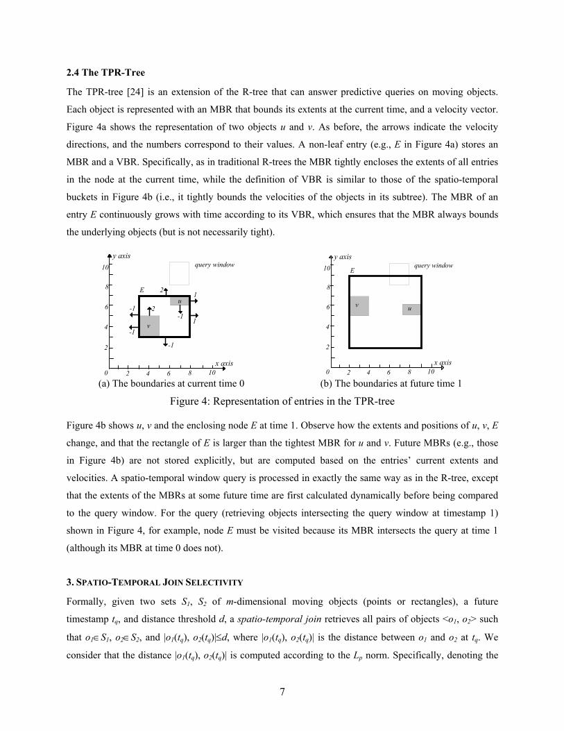
2.4 The TPR-Tree
The TPR-tree [24] is an extension of the R-tree that can answer predictive queries on moving objects.
Each object is represented with an MBR that bounds its extents at the current time, and a velocity vector.
Figure 4a shows the representation of two objects u and v. As before, the arrows indicate the velocity
directions, and the numbers correspond to their values. A non-leaf entry (e.g., E in Figure 4a) stores an
MBR and a VBR. Specifically, as in traditional R-trees the MBR tightly encloses the extents of all entries
in the node at the current time, while the definition of VBR is similar to those of the spatio-temporal
buckets in Figure 4b (i.e., it tightly bounds the velocities of the objects in its subtree). The MBR of an
entry E continuously grows with time according to its VBR, which ensures that the MBR always bounds
the underlying objects (but is not necessarily tight).
20 4 6 8 10
2
4
6
8
10
x axis
y axis
v
E
2-1
2
1
-1
query window
-1
u
-1
1
20 4 6 8 10
2
4
6
8
10
x axis
y axis
v
E
u
query window
(a) The boundaries at current time 0 (b) The boundaries at future time 1
Figure 4: Representation of entries in the TPR-tree
Figure 4b shows u, v and the enclosing node E at time 1. Observe how the extents and positions of u, v, E
change, and that the rectangle of E is larger than the tightest MBR for u and v. Future MBRs (e.g., those
in Figure 4b) are not stored explicitly, but are computed based on the entries’ current extents and
velocities. A spatio-temporal window query is processed in exactly the same way as in the R-tree, except
that the extents of the MBRs at some future time are first calculated dynamically before being compared
to the query window. For the query (retrieving objects intersecting the query window at timestamp 1)
shown in Figure 4, for example, node E must be visited because its MBR intersects the query at time 1
(although its MBR at time 0 does not).
3. SPATIO-TEMPORAL JOIN SELECTIVITY
Formally, given two sets S1, S2 of m-dimensional moving objects (points or rectangles), a future
timestamp tq, and distance threshold d, a spatio-temporal join retrieves all pairs of objects <o1, o2> such
that o1∈S1, o2∈S2, and |o1(tq), o2(tq)|≤d, where |o1(tq), o2(tq)| is the distance between o1 and o2 at tq. We
consider that the distance |o1(tq), o2(tq)| is computed according to the Lp norm. Specifically, denoting the
8
coordinates of an m-dimensional point p as p.x0, p.x1, …, p.xm, the Lp-distance |o1(tq), o2(tq)| equals
(∑i=1~d|p1.xi−p2.xi|p)1/p. A constrained spatio-temporal join is similar to a normal spatio-temporal join,
except that it involves a constraint window Wq which is an m-dimensional rectangle. A pair of qualifying
objects <o1, o2> must satisfy all the conditions of a normal join, and the additional predicate that o1 and o2
both intersect Wq at time tq. The selectivity of the (normal or constrained) join is the ratio between the
number of result pairs and the size of the Cartesian product S1×S2.
Interestingly, as discussed in [9], the join selectivity under various Lp norms (for different p) differs
only by a constant factor. As a result, to deal with arbitrary Lp norm, it suffices to solve the problem under
a particular value of p. In the sequel, we focus on L∞ (i.e., |o1(tq), o2(tq)| =maxi=1,2,…,m|p1.xi−p2.xi|), since the
resulting equations are the simplest in this case. The distance between two (hyper-) rectangles r1, r2 is the
minimum of the distances between all pairs of points in r1 and r2 respectively, or more formally: |r1,
r2|=min{|p1, p2| for all p1∈r1, and p2∈r2}. Under L∞, two (point or rectangle) objects o1, o2 are within
distance d if and only if the extended region of o1, obtained by enlarging its extents with length d along all
dimensions, intersects o2. Figure 5a and b illustrate this for 2D points and rectangles, respectively. When
d=0, the condition |o1(tq), o2(tq)|≤d reduces to simple intersection.
d
d d
d
p1
p2
extended region of p1
d
d
r2
d
d r1
extended region of r1
(a) Points (b) Rectangles
Figure 5: Objects within distance d (the L∞ norm) from each other
We use R1 (V1) to represent the MBR (VBR) that tightly encloses the location (velocities) of all the
objects in S1, and similarly, R2 (V2) for S2. Note that, R1 and R2 may cover different sub-spaces of the
universe (i.e., we allow objects of the two sets to distribute in different areas). The objective is to predict
the join selectivity based solely on R1, R2, V1, V2, assuming that (i) the location of the objects inside S1 (S2)
distributes uniformly in R1 (R2), (ii) the object velocities are uniform in V1 (V2), and (iii) all the
dimensions are independent. Section 3.1 first solves the problem for one-dimensional space, and Section
3.2 extends the results to higher-dimensionality, both assuming L∞. Section 3.3 extends the results to the
constrained join and other Lp norms. In Section 4 we overcome the uniformity assumptions with the aid of
histograms. Table 1 lists the symbols that will appear frequently in our analysis.
9
Symbol Description M dimensionality of the data space tq the query timestamp
S1, S2 The two datasets participating the join R1 (R2) The MBR of S1 (S2) covering the location of objects in the set V1 (V2) The VBRs of S1 (S2) covering the velocities of objects in the set N1 (N2) The number of objects in S1 (S2)
p.xi The i-th coordinate of point p [R.xi-, R.xi+] The extent along the i-th dimension of MBR R [V.vi-, V.vi+] The extent along the i-th dimension of VBR V
PQ{1Dpt, 1Dintv} The qualifying probability for 1D {point, interval} objects Sel{1Dpt,1Dintv, pt, rect} The join selectivity for {1D points, 1D intervals, mD points, mD rectangles}
Wq The constrained window
Table 1: Frequent symbols in the analysis
3.1 Solution for One-Dimensional Space
We first consider the case of 1D point data and then solve the problem for 1D intervals. Let [R1.x-, R1.x+]
be the extent of R1 (the MBR of S1), and [V1.v-, V1.v+] the range of V1 (the VBR of S1). The Cartesian
product S1×S2 consists of N1·N2 pairs of points. Let PQ1Dpt be the probability for a pair to qualify the join
condition; the expected number of qualifying pairs can be represented as N1·N2·PQ1Dpt. Furthermore, since
the selectivity equals the number of qualifying pairs divided by N1·N2, PQ1Dpt directly corresponds to the
join selectivity. In particular, the derivation of PQ1Dpt is equivalent to the following problem: Given two
points p1, p2 such that p1 (p2) uniformly distributes in the range [R1.x-, R1.x+] ([R2.x-, R2.x+]), and the
velocity of p1 (p2) uniformly distributes in [V1.v-, V1.v+] ([V2.v-, V2.v+]), compute the probability PQ1Dpt
that |p1(tq), p2(tq)|≤d.
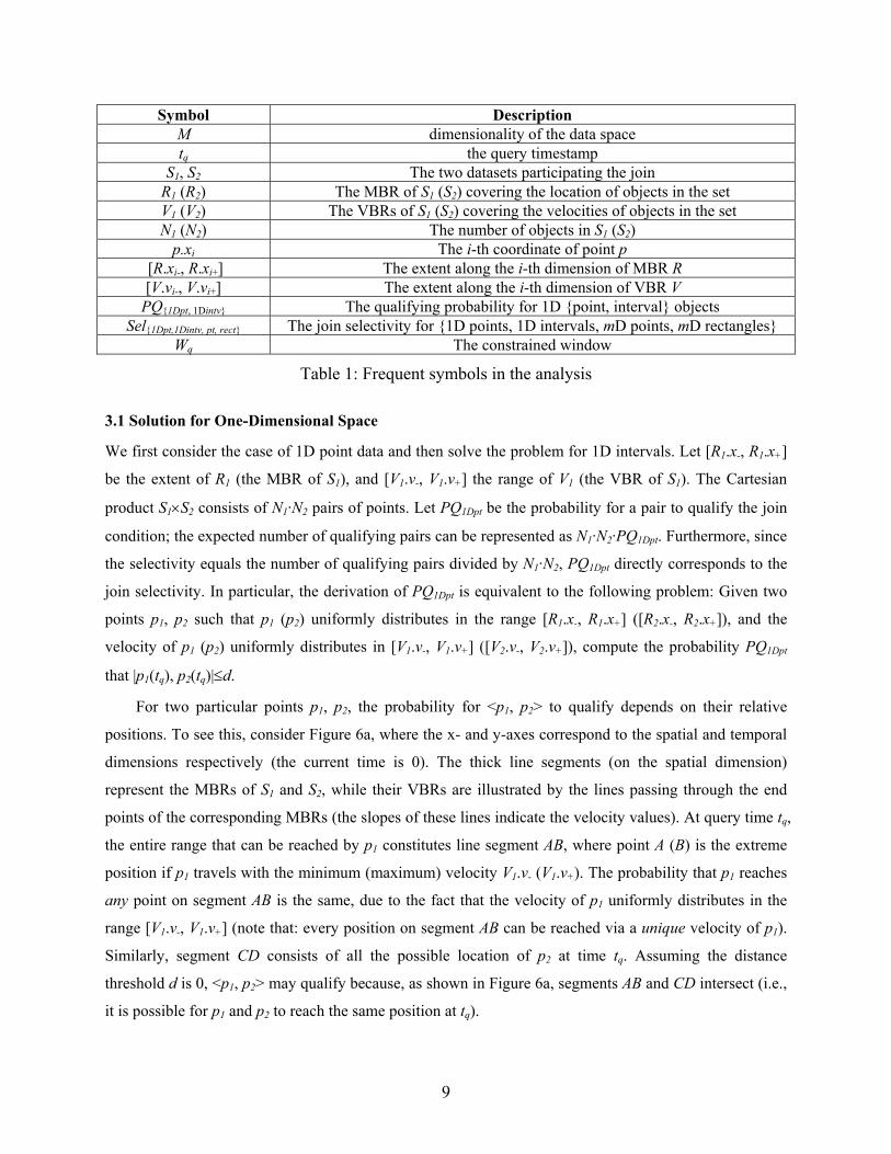
For two particular points p1, p2, the probability for <p1, p2> to qualify depends on their relative
positions. To see this, consider Figure 6a, where the x- and y-axes correspond to the spatial and temporal
dimensions respectively (the current time is 0). The thick line segments (on the spatial dimension)
represent the MBRs of S1 and S2, while their VBRs are illustrated by the lines passing through the end
points of the corresponding MBRs (the slopes of these lines indicate the velocity values). At query time tq,
the entire range that can be reached by p1 constitutes line segment AB, where point A (B) is the extreme
position if p1 travels with the minimum (maximum) velocity V1.v- (V1.v+). The probability that p1 reaches
any point on segment AB is the same, due to the fact that the velocity of p1 uniformly distributes in the
range [V1.v-, V1.v+] (note that: every position on segment AB can be reached via a unique velocity of p1).
Similarly, segment CD consists of all the possible location of p2 at time tq. Assuming the distance
threshold d is 0, <p1, p2> may qualify because, as shown in Figure 6a, segments AB and CD intersect (i.e.,
it is possible for p1 and p2 to reach the same position at tq).
10
R1.x- R1.x+ R2.x- R2.x+
V1.v- V1.v+V2.v - V2.v+
time
p1
p2
tq
A BC D
S1 .MBR S2 .MBR
spatial0histogram building time
spatial
time
p1 p
2
A B C D
S1 .MBR S2 .MBR
V1.v- V2.v+V1.v+V2.v -
R1.x- R1.x+ R2.x- R2.x+0
histogram building time
tq
(a) <p1, p2> may qualify (b) <p1, p2> cannot qualify
Figure 6: Qualifying pairs (distance threshold d=0)
Figure 6b shows similar situation except that p1 and p2 are farther apart from each other at the current time.
Notice that, in this case AB and CD do not intersect, indicating that <p1, p2> does not belong to the result.
Motivated by this, we denote with Ppair(l1, l2) the probability that pair <p1, p2> qualifies if p1 (p2) lies at
location l1 (l2). Consequently, the qualifying probability PQ1Dpt corresponds to the average of Ppair(l1, l2)
over all possible positions for l1 and l2, or formally:
( )( ) ( )1 2
1 2
. .
1 1 2 2 11 1 2 2 . .
1,
. . . .
R x R x
Dpt pair
R x R x
PQ P l l dl dlR x R x R x R x
+ +
− −+ − + −
=− − ∫ ∫ (1)
Given two points at l1 and l2 respectively, Ppair(l1, l2) corresponds to P{|p1(tq), p2(tq)|≤d}, i.e., the
probability that the distance of p1 and p2 at time tq is not greater than the threshold d. Assuming the
velocities of p1 and p2 to be u1 and u2 respectively, p1(tq) and p2(tq) can be represented as:
( )1 1 1q qp t l t u= + ⋅ , and ( )2 2 2q qp t l t u= + ⋅
Thus, ( ) ( ) ( ){ } ( ) ( ){ }1 2 1 2 1 1 2 2 1 2 1 2, ,pair q q qP l l P p t p t d p l and p l P l l t u u d= ≤ = = = − + ⋅ − ≤
The above equation can be converted to:
( ) 1 2 1 21 2 1 2 1,pair
q q
l l d l l dP l l P u u u
t t
⎧ ⎫− − − +⎪ ⎪= + ≤ ≤ +⎨ ⎬⎪ ⎪⎩ ⎭
(2)
Since u1 and u2 uniformly distribute in [V1.v-, V1.v+] and [V2.v-, V2.v+] respectively, they satisfy the
following probability density functions:
11 1
1( )
. .f u
V v V v+ −
=−
, and 2
2 2
1( )
. .f u
V v V v+ −
=−
Therefore, the right hand side of equation 2 can be written as3:
3 In this paper we follow the convention that if a>b, then ( ) 0
b
af x dx =∫ .
11
( ) ( )( )
( )
( )
1 22 1
1
1 1 22 1
min . ,.
1 2 1 21 2 1 1 2 2 1
.max . ,
1 1 2
1
. . .
q
q
l l dV v u tV v
q q V v l l dV v u t
l l d l l dP u u u f u f u du du
t t
V v V v V v
++
−−
⎛ ⎞− ++⎜ ⎟⎝ ⎠
⎛ ⎞− −+⎜ ⎟⎝ ⎠
+ − +
⎧ ⎫⎡ ⎤⎧ ⎫ ⎪ ⎪⎢ ⎥− − − +⎪ ⎪ ⎪ ⎪+ ≤ ≤ + =⎨ ⎬ ⎨ ⎬⎢ ⎥⎪ ⎪ ⎪ ⎪⎩ ⎭ ⎢ ⎥
⎪ ⎪⎣ ⎦⎩ ⎭
=−
∫ ∫
( ) ( )
( )1 22 1
1
1 1 22 1
min . ,.
2 12 .
max . ,
1.
q
q
l l dV v u tV v
V v l l dV v u t
du duV v
++
−−
⎛ ⎞− ++⎜ ⎟⎝ ⎠
− ⎛ ⎞− −+⎜ ⎟⎝ ⎠
− ∫ ∫
(3)
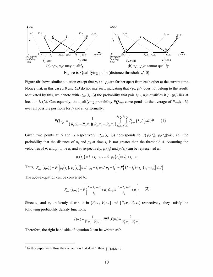
The above integral can be solved into closed form as presented in the appendix. To understand the
formula, consider Figure 7, where point p1(tq) shows the location of p1 at tq when it travels at speed u1
(∈[V1.v-, V1.v+]). Then, line segment AB corresponds to the set of positions for a qualifying point p2 at
time tq (i.e., p2(tq) is within distance d from p1(tq)).
V1.v- V1.v+ V2.v- V2.v+
time
p1
p2
d d
(p1 t )q
u1
u2max
u2min
spatial_l
2 l1
A B
histogram building time
0
tq
Figure 7: Computing the probability Ppair(l1, l2)
Let u2min and u2max be the velocities according to which p2 reaches points A and B at time tq respectively. It
follows that the probability that <p1, p2> is a join result, is (u2max−u2min)/(V2.v+−V2.v-), i.e., the probability
that the velocity u2 of p2 falls in the range [u2min, u2max], given that u2 uniformly distributes in [V2.v-, V2.v+].
So far we have considered a particular value of u1, while, as shown in equation 3, in order to compute
Ppair(l1, l2) we must consider all possible values in [V1.v-, V1.v+] (i.e., the outer integral in the formula).
Combining equations 1, -2, -3, we have represented PQ1Dpt as a function of R1, R2, V1, V2; the following
equation gives the complete formula for join selectivity of 1D points:
( )
( )( )( )( ) ( )
( )1 22 1
1 2 1
1 2 1 1 22 1
1
min . ,. . .
2 1 2 11 1 2 2 1 1 2 2 . . .
max . ,
,
11
. . . . . . . .
q
q
D pt q
l l dV v u tR x R x V v
R x R x V v l l dV v u t
Sel d t
du du dl dlR x R x R x R x V v V v V v V v
++ + +
− − −−
−
⎛ ⎞− ++⎜ ⎟⎝ ⎠
+ − + − + − + − ⎛ ⎞− −+⎜ ⎟⎝ ⎠
=
− − − − ∫ ∫ ∫ ∫ (4)
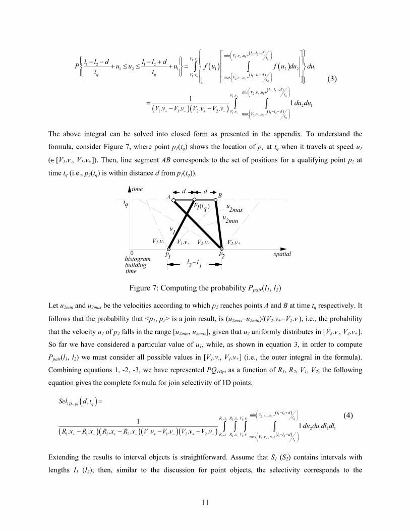
Extending the results to interval objects is straightforward. Assume that S1 (S2) contains intervals with
lengths I1 (I2); then, similar to the discussion for point objects, the selectivity corresponds to the
12
qualifying probability PQ1Dintv that a pair of intervals <i1, i2> in the cartesian product S1×S2 has distance
no longer than d at future time tq. Observe that i1 and i2 are closer than d, if and only if their centroids are
within distance d+(I1+I1)/2. This is illustrated in Figure 8, where intervals i1 and i2 (with lengths I1 and I2)
travel at velocities u1 and u2 respectively. Therefore, the selectivity PQ1Dintv can be estimated using
equation 4, except that, as shown in equation 5, (i) d should be replaced with d+(I1+I1)/2, and (ii) the
lower/upper limit of the integral should be modified to capture the fact that the centroid of i1 distributes in
[R1.x−+I1/2, R1.x+−I1/2] (the range is [R2.x−+I2/2, R2.x+−I2/2] for i2).
( ) ( )( )( )( )
( )
( )1 2 1 22 2 12 1
1 2 1 1 2 1 22 1
2
1 1 2 11 1 2 2 1 1 2 2
/ 2 / 2. min . ,/ 2 .
2 1 2 1
. . . / 2 / 2max . ,/ 2
1, , ,
. . . . . . . .
1q
q
D intv q Dintv
l l d I IR x V v u tI V v
R x R x V v l l d I IV v uI t
Sel d I I t PQR x R x R x R x V v V v V v V v
du du dl dl
+ ++
− − −−
−+ − + − + − + −
⎛ ⎞− + + ++⎜ ⎟− ⎝ ⎠
⎛ ⎞− − − −+⎜ ⎟+ ⎝ ⎠
= =− − − −
∫ ∫ ∫1
1
1
./ 2
/ 2
R xI
I
+−
+
∫
(5)
time
i1
i2
qt
d
i )(2 tq
spatial
(i1 t )q
I1
I2
d I1
I2
+ )/2+(
u1
u2
Figure 8: A pair of qualifying intervals
3.2 Arbitrary Dimensionality
In this section we present the equations for spatio-temporal join selectivity in m-dimensional spaces,
starting with point datasets before extending the results to rectangles. The MBR R1 (VBR V1) of set S1 is
now an m-dimensional rectangle, and its extent along the i-th dimension (1≤i≤m) is [R1.xi-, R1.xi+] ([V1.vi-,
V1.vi+]); similar notations are used for S2. Let PQpt be the probability that a pair of points <p1, p2> in S1×S2
satisfies the join condition. The crucial observation is that (due to the definition of L∞) |p1(tq), p2(tq)|≤d if
and only if |p1.xi(tq)−p2.xi(tq)|≤d for all dimensions 1≤i≤m, where p1.xi(tq) represents the i-th coordinate of
p1 at time tq. Let PQ1Dpt-i (1≤i≤m) be the probability that the ith coordinates of p1 and p2 qualify. Since the
dimensions are independent, we have:
11
m
pt Dpt ii
PQ PQ −=
=∏ (6)
The computation of PQ1Dpt-i along each dimension is based on equation 4 (passing d, tq), except that R1.x-,
R1.x+, V1.v-, V1.v+ should be replaced with R1.xi-, R1.xi+, V1.vi-, and V1.vi+ respectively. As in the 1D case,
PQpt corresponds to the selectivity Selpoint(d, tq, m).
13
In order to estimate the join selectivity for rectangular objects, we denote I1i (I2i) as the extents of the
objects in S1 (S2) along the i-th dimension. Given a pair of rectangles <r1, r2>, let their extents (on the i-th
dimension) at time tq be r1.ii(tq) and r2.ii(tq), respectively. In analogy with the point case, <r1, r2> is a join
result if and only if <r1.ii(tq), r2.ii(tq)> qualifies along the ith dimension (1≤i≤m), or equivalently, |r1.ii(tq),
r2.ii(tq)|≤d. Hence, the selectivity for m-dimensional rectangles is represented as:
( ) 11
, ,m
rect q Dintv ii
Sel d t m PQ −=
=∏ (7)
where PQ1Dintv-i is the probability that <r1.ii(tq), r2.ii(tq)> qualifies, and is computed according to equation
5 (passing d, I1i, I2i, and tq).
3.3 Extensions
In this section, we first study the selectivity estimation for constrained joins (again for L∞ metric), and
then explain the extension to arbitrary Lp norms. Our analysis of the constrained join follows the same
framework as the discussion on normal joins. Specifically, we first solve the fundamental problem
involving 1D points, and then tackle the general version (multi-dimensional, rectangle data) by reducing it
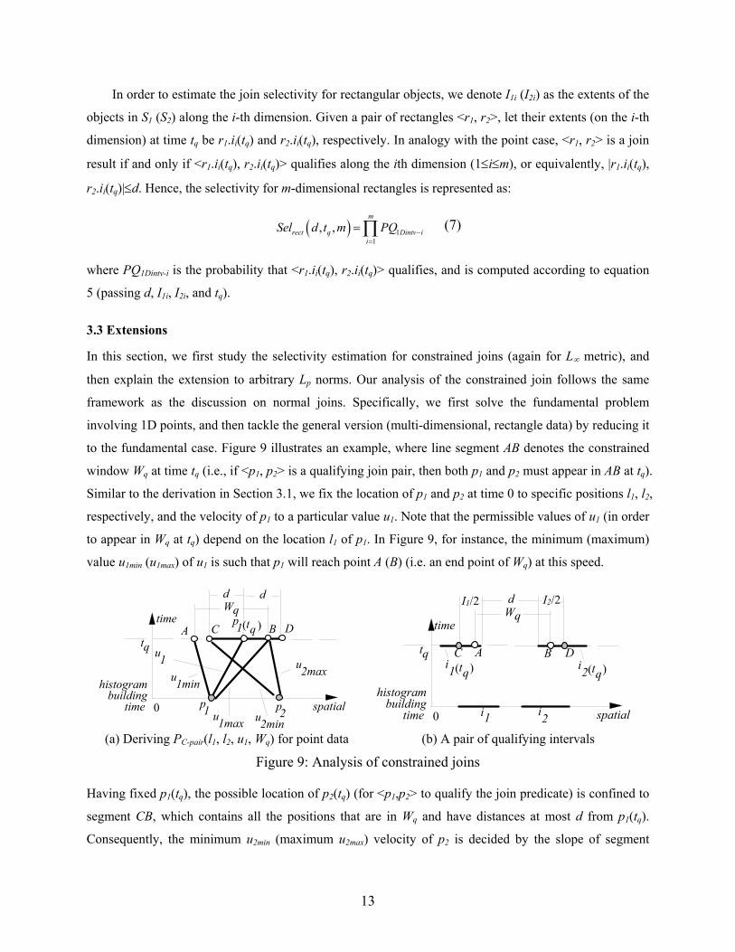
to the fundamental case. Figure 9 illustrates an example, where line segment AB denotes the constrained
window Wq at time tq (i.e., if <p1, p2> is a qualifying join pair, then both p1 and p2 must appear in AB at tq).
Similar to the derivation in Section 3.1, we fix the location of p1 and p2 at time 0 to specific positions l1, l2,
respectively, and the velocity of p1 to a particular value u1. Note that the permissible values of u1 (in order
to appear in Wq at tq) depend on the location l1 of p1. In Figure 9, for instance, the minimum (maximum)
value u1min (u1max) of u1 is such that p1 will reach point A (B) (i.e. an end point of Wq) at this speed.
time
spatial
histogrambuilding
time 0
tq
p1 p
2
(p1 t )q
u1 u
2max
u2min
A B
dWq
u1min
u1max
C D
d
time
spatial
histogrambuilding
time 0
tq
i1 i2
A B
dWq
C D
I1/2 I2/2
i )(2 tqi )(1 tq
(a) Deriving PC-pair(l1, l2, u1, Wq) for point data (b) A pair of qualifying intervals
Figure 9: Analysis of constrained joins
Having fixed p1(tq), the possible location of p2(tq) (for <p1,p2> to qualify the join predicate) is confined to
segment CB, which contains all the positions that are in Wq and have distances at most d from p1(tq).
Consequently, the minimum u2min (maximum u2max) velocity of p2 is decided by the slope of segment
14
connecting p2 and C (B). Therefore, the probability PC-pair(l1, l2, u1, Wq) that <p1, p2> qualifies (given l1, l2,
u1) equals (min(V2.v+, u2max)−max(V2.v−, u2min))/(u2max−u2min), taking into account the fact that u2 is in [u2min,
u2max]. Similar to the discussion in Section 3.1, the overall probability PC-1Dpt (i.e., the selectivity SelC-1Dpt)
can be obtained by integrating PC-pair(l1, l2, u1, Wq) over all the possible values for l1, l2, u1, as shown in
equation (8):
( ) ( ) ( )( )( )( )
( ) ( )( )1max1 2
1 2 1min
1 11 1 2 2 1 1 2 2
. .
2 2max 2 2min 1 2 1
. .
1, , , ,
. . . . . . . .
min . , max . ,
C Dpt q q C Dpt q q
uR x R x
R x R x u
Sel d t W P d t WR x R x R x R x V v V v V v V v
V v u V v u du dl dl+ +
− −
− −+ − + − + − + −
+
= =− − − −
− −∫ ∫ ∫ (8)
Next we study constrained joins on 1D intervals. Figure 9 shows two intervals i1, i2 (with lengths I1, I2,
respectively) that qualify the join (note that both i1(tq) and i2(tq) intersect the constraint region Wq). The
crucial observation is that, the centroids of i1, i2 must satisfy the following conditions: (i) the distance
between them is within d+(I1+I2)/2 (similar to Figure 8), and (ii) the centroid of i1 (i2) should have
distance no more than Wq/2+I1/2 (Wq/2+I2/2) from the centroid of Wq in order for i1(tq) (i2(tq)) to intersect
Wq. Hence, the selectivity for intervals can be reduced to equation 8 by considering the interval centroids
(as with equation 5, the integral ranges must be modified to ensure that both i1 and i2 lie in R1 and R2,
respectively). The extension to multiple dimensions is trivial: we simply multiply the selectivity on each
individual axis, as shown in Section 3.2.
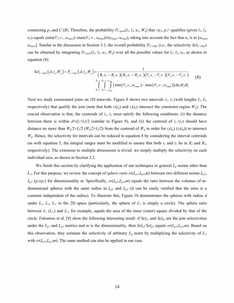
We finish this section by clarifying the application of our techniques to general Lp norms other than
L∞. For this purpose, we review the concept of sphere ratio sr(Lp1,Lp2,m) between two different norms Lp1,
Lp2 (p1≠p2) for dimensionality m. Specifically, sr(Lp1,Lp2,m) equals the ratio between the volumes of m-
dimensional spheres with the same radius in Lp1 and Lp2 (it can be easily verified that the ratio is a
constant independent of the radius). To illustrate this, Figure 10 demonstrates the spheres with radius d
under L1, L2, L∞ in the 2D space (particularly, the sphere of L2 is simply a circle). The sphere ratio
between L1 (L∞) and L2, for example, equals the area of the inner (outer) square divided by that of the
circle. Faloutsos et al. [9] show the following interesting result: if Selp1 and Selp2 are the join selectivities
under the Lp1 and Lp2 metrics and m is the dimensionality, then Selp1/Selp2 equals sr(Lp1,Lp2,m). Based on
this observation, they estimate the selectivity of arbitrary Lp norm by multiplying the selectivity of L∞
with sr(Lp1,Lp2,m). The same method can also be applied in our case.
15
Figure 10: Spheres in L1, L2, L∞ norms
4. SPATIO-TEMPORAL HISTOGRAMS
In the previous section we presented the formulae for estimating the join selectivity for datasets where
objects’ location and velocities distribute uniformly in their corresponding ranges. The uniformity
assumption, however, does not usually hold in real datasets, and thus direct application of the above
models will lead to significant error. In this section we deal with this problem using histograms that
partition the universe into separate buckets, such that the data distribution within a bucket is nearly
uniform. Then, the previous equations are applied locally (in each bucket), and the overall prediction is
obtained by summing up the individual estimations. The accuracy of this approach depends on the quality
of the histogram, which must guarantee that in each bucket both the location and the velocity distributions
are as uniform as possible. In Section 4.1, we first show that existing histograms cannot achieve this (thus,
leading to erroneous estimation), and then provide an alternative solution to avoid their defects. Section
4.2 explains how to use the proposed histogram to perform estimation, as well as various approaches to
reduce the computation cost.
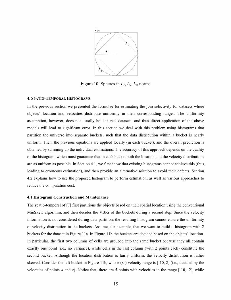
4.1 Histogram Construction and Maintenance
The spatio-temporal of [7] first partitions the objects based on their spatial location using the conventional
MinSkew algorithm, and then decides the VBRs of the buckets during a second step. Since the velocity
information is not considered during data partition, the resulting histogram cannot ensure the uniformity
of velocity distribution in the buckets. Assume, for example, that we want to build a histogram with 2
buckets for the dataset in Figure 11a. In Figure 11b the buckets are decided based on the objects’ location.
In particular, the first two columns of cells are grouped into the same bucket because they all contain
exactly one point (i.e., no variance), while cells in the last column (with 2 points each) constitute the
second bucket. Although the location distribution is fairly uniform, the velocity distribution is rather
skewed. Consider the left bucket in Figure 11b, whose (x-) velocity range is [-10, 8] (i.e., decided by the
velocities of points a and e). Notice that, there are 5 points with velocities in the range [-10, -2], while
16
only one (i.e., e) has positive velocity (8). Similarly, the velocity range of the right bucket is [-8, 10], but
ranges [-8, 0] and [2, 10] contain 2 and 4 points.
8
a
c
d
e
f
g
h
i
-10
-8
-6 -4
-2
-6
-8
2
6
4
b
k
l
j 10
8
a
c
d
e
f
g
h
i
-10
-8
-6 -4
-2
-6
-8
2
6
4
b
k
l
j 10
8
a
c
d
e
f
g
h
i
-10
-8
-6 -4
-2
-6
-8
2
6
4
b
k
l
j 10
(a) Cell information (b) Considering only location (c) Location and velocity
Figure 11: Uniform velocity distribution
An effective spatio-temporal histogram should partition data using both location and velocity information.
Continuing the previous example, Figure 11c shows such a histogram, where the left and right buckets
contain the first and the last two columns of cells respectively. Compared with Figure 11b, the spatial
uniformity is slightly worse (only in the right bucket), while the velocity uniformity is significantly better.
Specifically, the velocities distribute uniformly in the ranges [-10, -6] and [-8, 10] for the two buckets,
respectively. As a result, the new histogram is expected to produce better prediction.
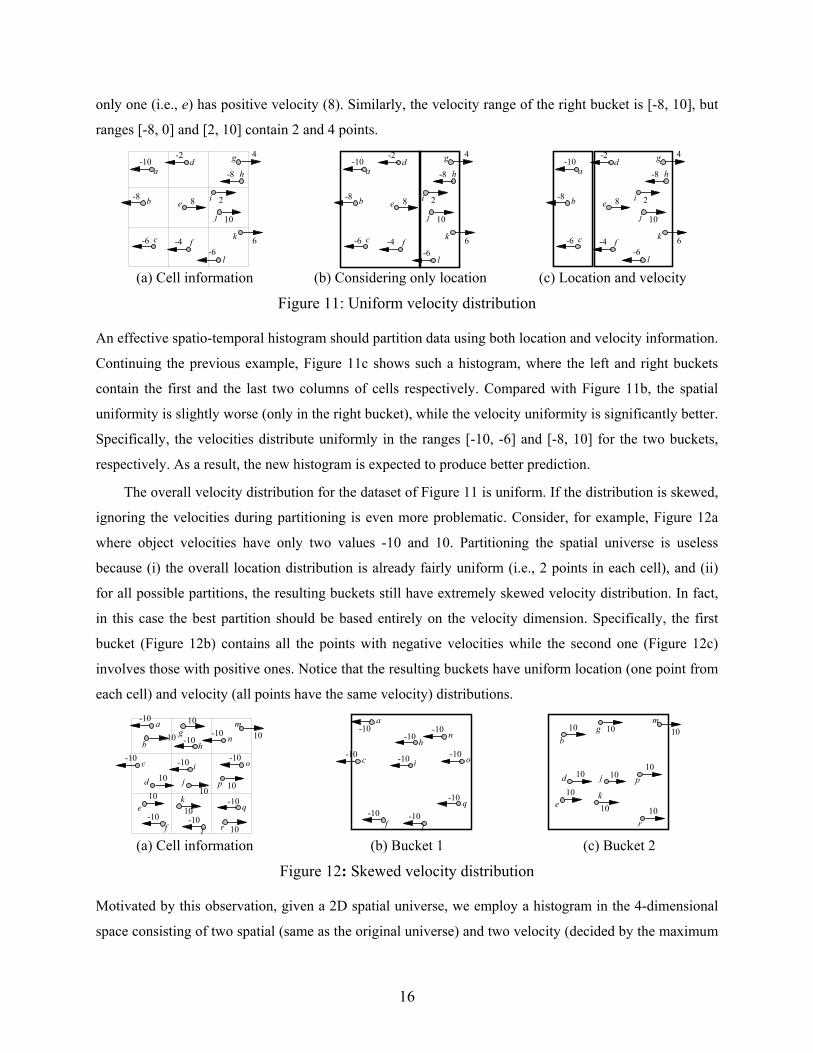
The overall velocity distribution for the dataset of Figure 11 is uniform. If the distribution is skewed,
ignoring the velocities during partitioning is even more problematic. Consider, for example, Figure 12a
where object velocities have only two values -10 and 10. Partitioning the spatial universe is useless
because (i) the overall location distribution is already fairly uniform (i.e., 2 points in each cell), and (ii)
for all possible partitions, the resulting buckets still have extremely skewed velocity distribution. In fact,
in this case the best partition should be based entirely on the velocity dimension. Specifically, the first
bucket (Figure 12b) contains all the points with negative velocities while the second one (Figure 12c)
involves those with positive ones. Notice that the resulting buckets have uniform location (one point from
each cell) and velocity (all points have the same velocity) distributions.
a
f
h
i
k
m-10
10
-1010
-10
-10
d
q
p 10
10b
c-10
10e
10g
10j
l-10
n-10
o-10
r 10
-10
10
-10
a
f
h
i
-10
-10
-10
-10q
c-10
l-10
n-10
o-10
k
m
10
10
10
d p
10
10
b10g
10j
r
10
10e
(a) Cell information (b) Bucket 1 (c) Bucket 2
Figure 12: Skewed velocity distribution
Motivated by this observation, given a 2D spatial universe, we employ a histogram in the 4-dimensional
space consisting of two spatial (same as the original universe) and two velocity (decided by the maximum

17
and minimum velocities along the corresponding spatial axis) dimensions. Specifically, a point (p.x1, p.x2)
with velocities (p.v1, p.v2) is converted into a 4D point (p.x1, p.x2, p.v1, p.v2), and similarly a rectangle r is
transformed to a 4D one with the same extents on the spatial and velocity dimensions. The histogram is
constructed using the MinSkew algorithm with an initial grid that partitions the space into H4 regular cells.
Each bucket b is associated with b.MBR that encloses the MBRs of all the cells in b, and with b.VBR that
tightly bounds the cell VBRs. For point datasets, b.num records the number of 4D points in b. For
rectangle sets, b.num is the number of 4D rectangles whose centroids lie in b, and b.len (b.vlen) is the
average spatial (velocity) extents of these rectangles. The discussion generalizes to arbitrary
dimensionality in a straightforward manner.
An important property of the proposed histogram is that it can be incrementally maintained. Figure
13 illustrates this using point data with one space/velocity dimension (extending to higher dimensionality
and rectangles is straightforward). Figure 13a and b illustrate the bucket extents in the space-velocity and
space-time universe, respectively. Particularly, in the space-time universe, a velocity is represented as the
slope of a line. Consider point p which falls in bucket b2, given its current location (as shown in both
figures) and velocity (25). Assume that p generates a velocity change (to -10) at future time t (when its
location is p(t)). To decide the bucket affected by p(t) (in the histogram constructed at time 0), we find a
point p' (called the surrogate point) at time 0, such that p' will reach the same position p(t) with the
updated velocity (-10) of p. As shown in Figure 13b, p' is the intersection of the spatial axis and the line
with slope -10 that crosses p(t). The bucket affected by p(t) is the one (b3) that contains p' in the space-
velocity universe, as shown in Figure 13a. Since the new bucket b3 is different from the old one b2, the
histogram must be modified by decreasing b2.num and increasing b3.num (by 1). In some cases, the
surrogate point may fall outside the universe, in which case the boundary bucket needs to be enlarged. As
an example, the MBR of bucket b3 must be expanded to cover the surrogate point q' (of q) in Figure 13. It
is worth mentioning that, the VBR of the selected bucket for expansion includes the updated velocity of q'
(i.e., hence b4 is not expanded).
spatial
velocityb2
b1
b4
b3
10
0
20
30
-10
-20
p
p'
q
q'
time
t
spatial0
histogram building time
b2.MBR b4.MBRb3 .MBR &
p
p( )t
p'
b1 .MBR &
pV=25 pV'=10
q
q( )t
q'
qV=25 qV'=10
(a) The cells and buckets (b) Point p falls in a different bucket after update
Figure 13: Updating the histogram
18
An exhaustive scan over all buckets is necessary to identify the ones affected by an update. To avoid this,
we build an in-memory4 TPR-tree on the MBRs and VBRs of the buckets (stored at the leaf level of the
tree), so that the affected ones can be identified very quickly by performing a window query using the
information of p and p' respectively. Since, as with normal TPR-trees, the non-leaf levels account for a
fraction of the total size, the space overhead is very small (less than 15% in our implementation).
Similarly, building the tree after the histogram has been constructed requires less than 1% of the total
construction time. Furthermore, notice that for most updates (except those requiring expansion) the
bucket extents are not changed, and thus the TPR-tree only needs to be maintained infrequently.
Updating the histogram incrementally avoids the frequent histogram re-building, and hence reduces
the maintenance cost considerably. Whenever the system receives an object update, the new information
is intercepted to modify the histogram accordingly. However, the uniformity (in buckets) may gradually
deteriorate along with time as the data (location and velocity) distributions vary. When the distribution
changes significantly, the histogram eventually needs to be re-built in order to ensure satisfactory
estimation accuracy. In order to formulate such a re-building condition, notice that, if sufficient
distribution changes have accumulated, the histogram must have been modified many times. Therefore, a
simple heuristic to ensure satisfactory estimation accuracy is to re-construct the histogram when the
number of modifications reaches a certain threshold. As evaluated in the experiments, high prediction
precision can be achieved with a very large threshold which leads to only occasional re-building.
4.2 Performing Estimation with Histograms
Given the histograms H1 and H2 for datasets S1 and S2 respectively, the expected number of qualifying
join pairs can be obtained by summing up the results of bucket pairs from H1×H2. Specifically, for two
buckets bi, bj (bi∈H1 and bj∈H2), the number of result pairs produced from objects inside them is
bi.num·bj.num·Selij(d, tq, m), where Selij(d, tq, m) is computed using equations 6 (for points), and 7 (for
rectangles), by replacing Ri, Rj, Vi, Vj with bi.MBR, bj.MBR, bi.VBR, bj.VBR respectively. Thus, the join
selectivity can be estimated as:
( )( )
1 2
1 2
. . , ,
, , i j
i j ij qfor all bucketsb H and b H
q
b num b num Sel d t m
Sel d t mN N
∈ ∈
⋅ ⋅
=⋅
∑ (9)
where N1 and N2 are the cardinalities of S1 and S2 respectively.
4 As currently there is no version of the TPR-tree specifically designed for main memory, our implementation follows the disk-resident version, although with a different node size (=10). This choice of the node capacity is discussed towards the end of the section.
19
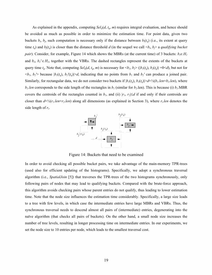
As explained in the appendix, computing Selij(d, tq, m) requires integral evaluation, and hence should
be avoided as much as possible in order to minimize the estimation time. For point data, given two
buckets bi, bj, such computation is necessary only if the distance between bi(tq) (i.e., its extent at query
time tq) and bj(tq) is closer than the distance threshold d (in the sequel we call <bi, bj> a qualifying bucket
pair). Consider, for example, Figure 14 which shows the MBRs (at the current time) of 3 buckets: b1∈H1
and b2, b2' ∈H2, together with the VBRs. The dashed rectangles represent the extents of the buckets at
query time tq. Note that, computing Selij(d, tq, m) is necessary for <b1, b2> (|b1(tq), b2(tq)| =0<d), but not for
<b1, b2'> because |b1(tq), b2'(tq)|>d, indicating that no points from b1 and b2' can produce a joined pair.
Similarly, for rectangular data, we do not consider two buckets if |b1(tq), b2(tq)|>d+½(b1.len+b2.len), where
b1.len corresponds to the side length of the rectangles in b1 (similar for b2.len). This is because (i) b1.MBR
covers the centroids of the rectangles counted in b1, and (ii) |r1, r2|≤d if and only if their centroids are
closer than d+½(r1.len+r2.len) along all dimensions (as explained in Section 3), where ri.len denotes the
side length of ri.
b1
(b1
tq)
b2
(b2
tq)b2
'
' (b2
tq)
d
Figure 14: Buckets that need to be examined
In order to avoid checking all possible bucket pairs, we take advantage of the main-memory TPR-trees
(used also for efficient updating of the histograms). Specifically, we adopt a synchronous traversal
algorithm (i.e., SpatialJoin [5]) that traverses the TPR-trees of the two histograms synchronously, only
following pairs of nodes that may lead to qualifying buckets. Compared with the brute-force approach,
this algorithm avoids checking pairs whose parent entries do not qualify, thus leading to lower estimation
time. Note that the node size influences the estimation time considerably. Specifically, a large size leads
to a tree with few levels, in which case the intermediate entries have large MBRs and VBRs. Thus, the
synchronous traversal needs to descend almost all pairs of (intermediate) entries, degenerating into the
naïve algorithm (that checks all pairs of buckets). On the other hand, a small node size increases the
number of tree levels, resulting in longer processing time on intermediate entries. In our experiments, we
set the node size to 10 entries per node, which leads to the smallest traversal cost.
20
5. EXPERIMENTS
In this section we present an extensive experimentation to prove the effectiveness of the proposed
methods. All experiments were performed using a Pentium IV 1GHz CPU with 256 Mbytes memory. Due
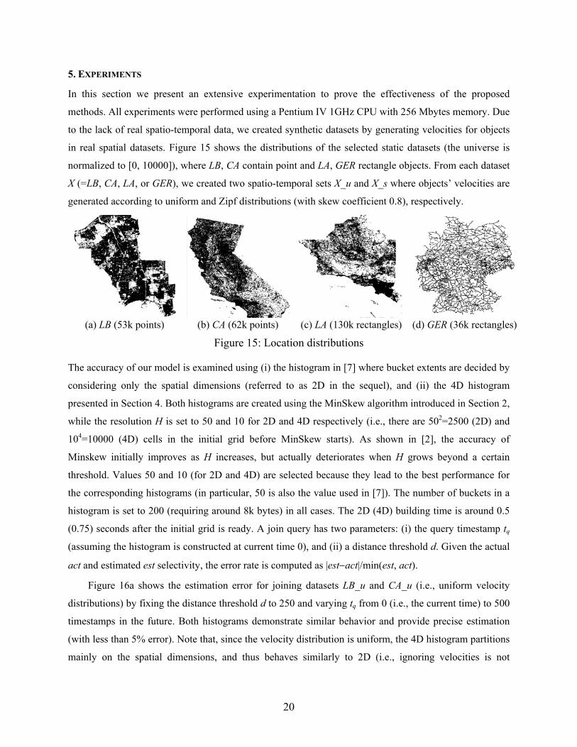
to the lack of real spatio-temporal data, we created synthetic datasets by generating velocities for objects
in real spatial datasets. Figure 15 shows the distributions of the selected static datasets (the universe is
normalized to [0, 10000]), where LB, CA contain point and LA, GER rectangle objects. From each dataset
X (=LB, CA, LA, or GER), we created two spatio-temporal sets X_u and X_s where objects’ velocities are
generated according to uniform and Zipf distributions (with skew coefficient 0.8), respectively.
(a) LB (53k points) (b) CA (62k points) (c) LA (130k rectangles) (d) GER (36k rectangles)
Figure 15: Location distributions
The accuracy of our model is examined using (i) the histogram in [7] where bucket extents are decided by
considering only the spatial dimensions (referred to as 2D in the sequel), and (ii) the 4D histogram
presented in Section 4. Both histograms are created using the MinSkew algorithm introduced in Section 2,
while the resolution H is set to 50 and 10 for 2D and 4D respectively (i.e., there are 502=2500 (2D) and
104=10000 (4D) cells in the initial grid before MinSkew starts). As shown in [2], the accuracy of
Minskew initially improves as H increases, but actually deteriorates when H grows beyond a certain
threshold. Values 50 and 10 (for 2D and 4D) are selected because they lead to the best performance for
the corresponding histograms (in particular, 50 is also the value used in [7]). The number of buckets in a
histogram is set to 200 (requiring around 8k bytes) in all cases. The 2D (4D) building time is around 0.5
(0.75) seconds after the initial grid is ready. A join query has two parameters: (i) the query timestamp tq
(assuming the histogram is constructed at current time 0), and (ii) a distance threshold d. Given the actual
act and estimated est selectivity, the error rate is computed as |est−act|/min(est, act).
Figure 16a shows the estimation error for joining datasets LB_u and CA_u (i.e., uniform velocity
distributions) by fixing the distance threshold d to 250 and varying tq from 0 (i.e., the current time) to 500
timestamps in the future. Both histograms demonstrate similar behavior and provide precise estimation
(with less than 5% error). Note that, since the velocity distribution is uniform, the 4D histogram partitions
mainly on the spatial dimensions, and thus behaves similarly to 2D (i.e., ignoring velocities is not
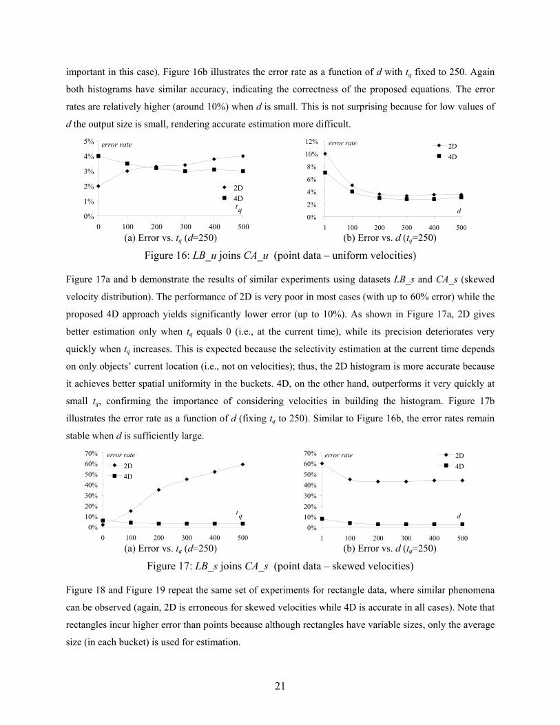
21
important in this case). Figure 16b illustrates the error rate as a function of d with tq fixed to 250. Again
both histograms have similar accuracy, indicating the correctness of the proposed equations. The error
rates are relatively higher (around 10%) when d is small. This is not surprising because for low values of
d the output size is small, rendering accurate estimation more difficult.
tq
error rate
0%
1%
2%
3%
4%
5%
0 100 200 300 400 500
2D
4D
2D
4D
d
error rate
0%
2%
4%
6%
8%
10%
12%
1 100 200 300 400 500 (a) Error vs. tq (d=250) (b) Error vs. d (tq=250)
Figure 16: LB_u joins CA_u (point data – uniform velocities)
Figure 17a and b demonstrate the results of similar experiments using datasets LB_s and CA_s (skewed
velocity distribution). The performance of 2D is very poor in most cases (with up to 60% error) while the
proposed 4D approach yields significantly lower error (up to 10%). As shown in Figure 17a, 2D gives
better estimation only when tq equals 0 (i.e., at the current time), while its precision deteriorates very
quickly when tq increases. This is expected because the selectivity estimation at the current time depends
on only objects’ current location (i.e., not on velocities); thus, the 2D histogram is more accurate because
it achieves better spatial uniformity in the buckets. 4D, on the other hand, outperforms it very quickly at
small tq, confirming the importance of considering velocities in building the histogram. Figure 17b
illustrates the error rate as a function of d (fixing tq to 250). Similar to Figure 16b, the error rates remain
stable when d is sufficiently large.
t q
error rate
0%
10%
20%
30%
40%
50%
60%
70%
0 100 200 300 400 500
2D
4D
d
error rate
0%
10%
20%
30%
40%
50%
60%
70%
1 100 200 300 400 500
2D
4D
(a) Error vs. tq (d=250) (b) Error vs. d (tq=250)
Figure 17: LB_s joins CA_s (point data – skewed velocities)
Figure 18 and Figure 19 repeat the same set of experiments for rectangle data, where similar phenomena
can be observed (again, 2D is erroneous for skewed velocities while 4D is accurate in all cases). Note that
rectangles incur higher error than points because although rectangles have variable sizes, only the average
size (in each bucket) is used for estimation.
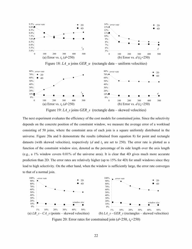
22
tq
error rate
5.0%5.5%6.0%6.5%7.0%7.5%8.0%8.5%9.0%9.5%
0 100 200 300 400 500
2D
4D
d
error rate
5%6%7%8%9%
10%11%12%13%14%
0 100 200 300 400 500
2D
4D
(a) Error vs. tq (d=250) (b) Error vs. d (tq=250)
Figure 18: LA_u joins GER_u (rectangle data – uniform velocities)
tq
error rate
0%
10%
20%30%
40%
50%
60%
70%80%
0 100 200 300 400 500
2D
4D
d
error rate
0%
10%
20%
30%
40%
50%
60%
70%
80%
0 100 200 300 400 500
2D
4D
(a) Error vs. tq (d=250) (b) Error vs. d (tq=250)
Figure 19: LA_s joins GER_s (rectangle data – skewed velocities)
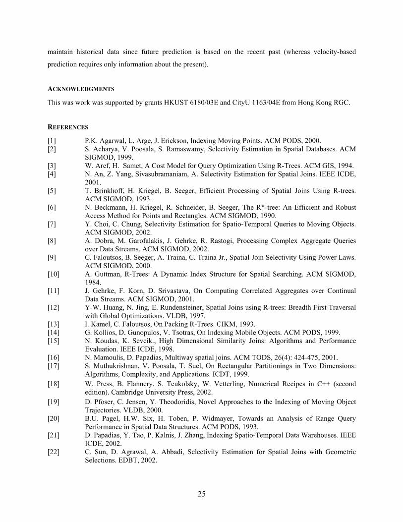
The next experiment evaluates the efficiency of the cost models for constrained joins. Since the selectivity
depends on the concrete position of the constraint window, we measure the average error of a workload
consisting of 50 joins, where the constraint area of each join is a square uniformly distributed in the
universe. Figure 20a and b demonstrate the results (obtained from equation 8) for point and rectangle
datasets (with skewed velocities), respectively (d and tq are set to 250). The error rate is plotted as a
function of the constraint window size, denoted as the percentage of its side length over the axis length
(e.g., a 1% window covers 0.01% of the universe area). It is clear that 4D gives much more accurate
prediction than 2D. The error rates are relatively higher (up to 15% for 4D) for small windows since they
lead to high selectivity. On the other hand, when the window is sufficiently large, the error rate converges
to that of a normal join.
error rate
0%10%20%30%40%50%60%70%80%90%
100%
1% 10% 20% 30% 40% 50%
2D
4D
window size
error rate
window size
0%10%20%30%40%50%60%70%80%90%
100%
1% 10% 20% 30% 40% 50%
2D
4D
(a) LB_s - CA_s (points – skewed velocities) (b) LA_s - GER_s (rectangles – skewed velocities)
Figure 20: Error rates for constrained join (d=250, tq=250)
23
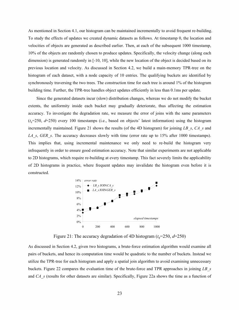
As mentioned in Section 4.1, our histogram can be maintained incrementally to avoid frequent re-building.
To study the effects of updates we created dynamic datasets as follows. At timestamp 0, the location and
velocities of objects are generated as described earlier. Then, at each of the subsequent 1000 timestamp,
10% of the objects are randomly chosen to produce updates. Specifically, the velocity change (along each
dimension) is generated randomly in [-10, 10], while the new location of the object is decided based on its
previous location and velocity. As discussed in Section 4.2, we build a main-memory TPR-tree on the
histogram of each dataset, with a node capacity of 10 entries. The qualifying buckets are identified by
synchronously traversing the two trees. The construction time for each tree is around 1% of the histogram
building time. Further, the TPR-tree handles object updates efficiently in less than 0.1ms per update.
Since the generated datasets incur (slow) distribution changes, whereas we do not modify the bucket
extents, the uniformity inside each bucket may gradually deteriorate, thus affecting the estimation
accuracy. To investigate the degradation rate, we measure the error of joins with the same parameters
(tq=250, d=250) every 100 timestamps (i.e., based on objects’ latest information) using the histogram
incrementally maintained. Figure 21 shows the results (of the 4D histogram) for joining LB_s, CA_s and
LA_s, GER_s. The accuracy decreases slowly with time (error rate up to 15% after 1000 timestamps).
This implies that, using incremental maintenance we only need to re-build the histogram very
infrequently in order to ensure good estimation accuracy. Note that similar experiments are not applicable
to 2D histograms, which require re-building at every timestamp. This fact severely limits the applicability
of 2D histograms in practice, where frequent updates may invalidate the histogram even before it is
constructed.
0%
2%
4%
6%
8%
10%
12%
14%
0 200 400 600 800 1000
error rate
elapsed timestamps
LB_s JOIN CA_s
LA_s JOIN GER_s
Figure 21: The accuracy degradation of 4D histogram (tq=250, d=250)
As discussed in Section 4.2, given two histograms, a brute-force estimation algorithm would examine all
pairs of buckets, and hence its computation time would be quadratic to the number of buckets. Instead we
utilize the TPR-tree for each histogram and apply a spatial join algorithm to avoid examining unnecessary
buckets. Figure 22 compares the evaluation time of the brute-force and TPR approaches in joining LB_s
and CA_s (results for other datasets are similar). Specifically, Figure 22a shows the time as a function of
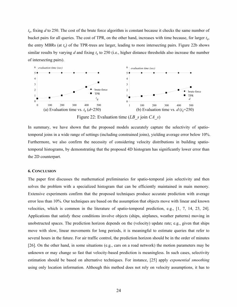
24
tq, fixing d to 250. The cost of the brute force algorithm is constant because it checks the same number of
bucket pairs for all queries. The cost of TPR, on the other hand, increases with time because, for larger tq,
the entry MBRs (at tq) of the TPR-trees are larger, leading to more intersecting pairs. Figure 22b shows
similar results by varying d and fixing tq to 250 (i.e., higher distance thresholds also increase the number
of intersecting pairs).
0
1
2
3
4
5
6
0 100 200 300 400 500
brute-force
TPR
tq
evaluation time (sec)
d
evaluation time (sec)
0
1
2
3
4
5
6
1 100 200 300 400 500
brute-force
TPR
(a) Evaluation time vs. tq (d=250) (b) Evaluation time vs. d (tq=250)
Figure 22: Evaluation time (LB_s join CA_s)
In summary, we have shown that the proposed models accurately capture the selectivity of spatio-
temporal joins in a wide range of settings (including constrained joins), yielding average error below 10%.
Furthermore, we also confirm the necessity of considering velocity distributions in building spatio-
temporal histograms, by demonstrating that the proposed 4D histogram has significantly lower error than
the 2D counterpart.
6. CONCLUSION
The paper first discusses the mathematical preliminaries for spatio-temporal join selectivity and then
solves the problem with a specialized histogram that can be efficiently maintained in main memory.
Extensive experiments confirm that the proposed techniques produce accurate prediction with average
error less than 10%. Our techniques are based on the assumption that objects move with linear and known
velocities, which is common in the literature of spatio-temporal prediction, e.g., [1, 7, 14, 23, 24].
Applications that satisfy these conditions involve objects (ships, airplanes, weather patterns) moving in
unobstructed spaces. The prediction horizon depends on the (velocity) update rate; e.g., given that ships
move with slow, linear movements for long periods, it is meaningful to estimate queries that refer to
several hours in the future. For air traffic control, the prediction horizon should be in the order of minutes
[26]. On the other hand, in some situations (e.g., cars on a road network) the motion parameters may be
unknown or may change so fast that velocity-based prediction is meaningless. In such cases, selectivity
estimation should be based on alternative techniques. For instance, [25] apply exponential smoothing
using only location information. Although this method does not rely on velocity assumptions, it has to
25
maintain historical data since future prediction is based on the recent past (whereas velocity-based
prediction requires only information about the present).
ACKNOWLEDGMENTS
This was work was supported by grants HKUST 6180/03E and CityU 1163/04E from Hong Kong RGC.
REFERENCES
[1] P.K. Agarwal, L. Arge, J. Erickson, Indexing Moving Points. ACM PODS, 2000. [2] S. Acharya, V. Poosala, S. Ramaswamy, Selectivity Estimation in Spatial Databases. ACM
SIGMOD, 1999. [3] W. Aref, H. Samet, A Cost Model for Query Optimization Using R-Trees. ACM GIS, 1994. [4] N. An, Z. Yang, Sivasubramaniam, A. Selectivity Estimation for Spatial Joins. IEEE ICDE,
2001. [5] T. Brinkhoff, H. Kriegel, B. Seeger, Efficient Processing of Spatial Joins Using R-trees.
ACM SIGMOD, 1993. [6] N. Beckmann, H. Kriegel, R. Schneider, B. Seeger, The R*-tree: An Efficient and Robust
Access Method for Points and Rectangles. ACM SIGMOD, 1990. [7] Y. Choi, C. Chung, Selectivity Estimation for Spatio-Temporal Queries to Moving Objects.
ACM SIGMOD, 2002. [8] A. Dobra, M. Garofalakis, J. Gehrke, R. Rastogi, Processing Complex Aggregate Queries
over Data Streams. ACM SIGMOD, 2002. [9] C. Faloutsos, B. Seeger, A. Traina, C. Traina Jr., Spatial Join Selectivity Using Power Laws.
ACM SIGMOD, 2000. [10] A. Guttman, R-Trees: A Dynamic Index Structure for Spatial Searching. ACM SIGMOD,
1984. [11] J. Gehrke, F. Korn, D. Srivastava, On Computing Correlated Aggregates over Continual
Data Streams. ACM SIGMOD, 2001. [12] Y-W. Huang, N. Jing, E. Rundensteiner, Spatial Joins using R-trees: Breadth First Traversal
with Global Optimizations. VLDB, 1997. [13] I. Kamel, C. Faloutsos, On Packing R-Trees. CIKM, 1993. [14] G. Kollios, D. Gunopulos, V. Tsotras, On Indexing Mobile Objects. ACM PODS, 1999. [15] N. Koudas, K. Sevcik., High Dimensional Similarity Joins: Algorithms and Performance
Evaluation. IEEE ICDE, 1998. [16] N. Mamoulis, D. Papadias, Multiway spatial joins. ACM TODS, 26(4): 424-475, 2001. [17] S. Muthukrishnan, V. Poosala, T. Suel, On Rectangular Partitionings in Two Dimensions:
Algorithms, Complexity, and Applications. ICDT, 1999. [18] W. Press, B. Flannery, S. Teukolsky, W. Vetterling, Numerical Recipes in C++ (second
edition). Cambridge University Press, 2002. [19] D. Pfoser, C. Jensen, Y. Theodoridis, Novel Approaches to the Indexing of Moving Object
Trajectories. VLDB, 2000. [20] B.U. Pagel, H.W. Six, H. Toben, P. Widmayer, Towards an Analysis of Range Query
Performance in Spatial Data Structures. ACM PODS, 1993. [21] D. Papadias, Y. Tao, P. Kalnis, J. Zhang, Indexing Spatio-Temporal Data Warehouses. IEEE
ICDE, 2002. [22] C. Sun, D. Agrawal, A. Abbadi, Selectivity Estimation for Spatial Joins with Geometric
Selections. EDBT, 2002.

26
[23] S. Saltenis, C.S. Jensen, Indexing of Moving Objects for Location-Based Services. IEEE ICDE, 2002.
[24] S. Saltenis, C.S. Jensen, S.T. Leutenegger, M.A. Lopez, Indexing the Positions of Continuously Moving Objects. ACM SIGMOD, 2000.
[25] J. Sun, D. Papadias, Y. Tao, B. Liu, Querying about the Past, the Present, and the Future in Spatio-Temporal Databases. IEEE ICDE, 2004.
[26] Y. Tao, J. Sun, D. Papadias, Analysis of Predictive Spatio-temporal Queries. ACM TODS, 28(4): 295-336, 2003.
[27] Y. Theodoridis, E. Stefanakis, T. Sellis, Cost Models for Join Queries in Spatial Databases. IEEE ICDE, 1998.
APPENDIX
This appendix discusses the evaluation of the integrals in equations 3 and 4. For the sake of simplicity, we
use the notation ( )1 2
q
l l dtα − −= and ( )1 2
q
l l dtβ − += ; thus, the integral in equation 3 can be written as
( )
( )2 11
1 2 1
min . ,.
2 1
. max . ,
1V v uV v
V v V v u
du duβ
α
++
− −
+
+∫ ∫ .
The value of the integral equals the area of the intersection (the shaded region in Figure 23a) of (i) the
rectangle bounded by lines {u1=V1.v-, u1=V1.v+, u2=V2.v-, u2=V1.v+}, and (ii) the region between parallel
lines LN1: u2=u1+α and LN2: u2=u1+β. As shown inFigure 23b and c, the shaded area is the difference of
areas Ar1 and Ar2, i.e., the intersection of the rectangle in (i) and the lower half planes of lines LN1 and
LN2 respectively. Obviously Ar1 depends on the intercept (i.e., α) of LN1, which decides the relative
positions of LN1 and the rectangle; Table A.1 illustrates its values for the all six possible cases. Due to the
symmetry, values of Ar2 (as well as the corresponding conditions) are the same as those in Table 1, except
that α should be replaced with β. Notice that since the integral in equation 3 equals Ar1−Ar2, we have
solved the equation into closed form.
u1=V1.v- u1=V1.v+
u2=V2.v-
u2=V2.v+
u2=u1+α
u2=u1+β
LN1
LN2
u1=V1.v- u1=V1.v+
u2=V2.v-
u2=V2.v+
u2=u1+α
u2=u1+β
LN1
LN2
u1=V1.v- u1=V1.v+
u2=V2.v-
u2=V2.v+
u2=u1+αLN1
LN2
(a) Integral area (b) Area Ar1 (c) Area Ar2
Figure 23: Integral area=Ar1−Ar2
Because the exact solution of equation 4 is more complex, in our implementation we evaluate it using the
trapezoidal method [18]. Particularly, the numerical approach is applied to the two outer integral layers
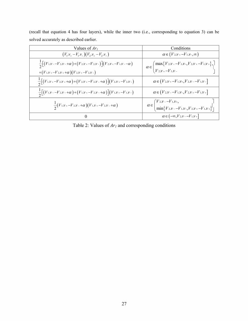
27
(recall that equation 4 has four layers), while the inner two (i.e., corresponding to equation 3) can be
solved accurately as described earlier.
Values of Ar1 Conditions
( )( )1 1 2 2. . . .V v V v V v V v+ − + −− − ( )2 1. . ,V v V vα + −∈ − ∞
( ) ( ) ( )
( )( )
1 2 2 2 2 1
1 2 2 2
1. . . . . .
2. . . .
V v V v V v V v V v V v
V v V v V v V v
α α
α
− − + − + −
+ + + −
⎡ ⎤− + + − − −⎣ ⎦
+ − + −
{ }2 1 2 1
2 1
max . . , . . ,
. .
V v V v V v V v
V v V vα
− − + +
+ −
⎛ ⎤− −∈⎜ ⎥
−⎝ ⎦
( ) ( ) ( )1 2 2 2 2 21
. . . . . .2
V v V v V v V v V v V vα α+ + + − + −⎡ ⎤− + + − + −⎣ ⎦ ( ]2 1 2 1. . , . .V v V v V v V vα + + − −∈ − −
( ) ( ) ( )1 2 1 2 1 11
. . . . . .2
V v V v V v V v V v V vα α− − + − + −⎡ ⎤− + + − + −⎣ ⎦ ( ]2 1 2 1. . , . .V v V v V v V vα − − + +∈ − −
( )( )1 2 1 21
. . . .2
V v V v V v V vα α+ − + −− + − + { }
2 1
2 1 2 1
. . ,
min . . , . .
V v V v
V v V v V v V vα
− +
− − + +
−⎛ ⎤∈⎜ ⎥− −⎝ ⎦
0 ( ]2 1, . .V v V vα − +∈ −∞ −
Table 2: Values of Ar1 and corresponding conditions