Applied Vegetation Science 19 (2016) 267–279

Spatial variation of fuel loading within varying aged stands of chaparral Kellie A. Uyeda, Douglas A. Stow, John F. O’Leary, Ian T. Schmidt & Philip J. Riggan

Keywords

Adenostoma fasciculatum; Biomass

accumulation; California chaparral; Chamise;

Post-fire recovery; Quercus berberidifolia;

Scrub oak; Shrub; Stand age; Vegetation type

map; Wildfire

Nomenclature

Baldwin et al. (2012)

Received 24 February 2015

Accepted 14 October 2015

Co-ordinating Editor: Norbert H€olzel

Uyeda, K.A. (corresponding author, kellie.

uyeda@gmail.com)1,2 ,

Stow, D.A. (stow@mail.sdsu.edu)1,

O’Leary, J.F. (oleary@mail.sdsu.edu)1,

Schmidt, I.T. (itssit@gmail.com)1,

Riggan, P.J. (priggan@fs.fed.us)3

1Department of Geography, San Diego State

University, 5500 Campanile Drive, San Diego,

CA, USA; 2Department of Geography, University of

California, 1832 Ellison Hall, Santa Barbara, CA

93106-4060, USA; 3Pacific Southwest Research Station, United

States Forest Service, 4955 Canyon Crest

Drive, Riverside, CA 92507, USA

Abstract

Questions: How do stand-level biomass and percentage of dead material in cha­parral vary as a function of stand age? How do the landscape properties of aggre­gation index and patch size vary in each of the dominant species groups as a function of stand age?

Location: Stands of 7-, 28- and 68-yr-old chaparral, San Diego County, CA, US.

Methods: We sampled and estimated above-ground biomass in 8 m 9 8 m field plots. Each stand was classified into species groups using high-resolution imagery. After establishing coefficients for the average biomass per area for each species group and stand age using field data, we estimated biomass in 30 random plots in each stand age using the classified map. We also estimated biomass using pooled coefficients (average of the 28- and 68-yr-old biomass per area). We cal­culated landscape metrics in six 60 m 9 60 m study sites for each stand age.

Results: While we found a statistically significant pattern of higher biomass in the older chaparral stands when using age-specific biomass coefficients, there was no statistical difference between the 28- and 68-yr-old stands using the more conservative pooled coefficients. Both approaches revealed a wide range in biomass in all age classes. We were not able to map dead biomass with suffi­cient accuracy to measure age-related differences, but no differences in the two older stands were obvious in the field. There were no significant differences in landscape metrics between the two older stands, and the differences observed in the younger stand might have been partially due to aspect differences.

Conclusions: Our approach of using a combination of field plots and classifica­tion of remote sensing imagery is a valuable method for enlarging the effective study area in chaparral, and allowed us to better measure how widely biomass varies across the study area. High spatial resolution measurements of fuel prop­erties could help support more detailed models of fire behaviour.

Introduction

In southern California chaparral shrublands, wildfires typi­cally occur as intense crown fires, with behaviour influ­enced by high temperatures, low humidity, high wind, terrain and biomass levels. The fires consume all above­ground biomass but the largest live stems in the thick stands of sclerophyllous shrubs. The first 3 to 4 yr follow­

ing a fire are characterized by an abundance of herbaceous vegetation, after which time shrubs become dominant and return to pre-fire cover levels within 10 to 15 yr (Keeley et al. 1981; McMichael et al. 2004). While shrub cover returns to pre-fire levels fairly rapidly, the amount of total above-ground biomass continues to increase with time

(Riggan et al. 1988). The rate of this accumulation declines with time within the first two decades of recovery, but there appears to be positive net accumulation at least until an age of approximately 40 yr (Rundel & Parsons 1979; Black 1987). After 40 yr, vegetation biomass tends to reach a steady state (Black 1987). These patterns of biomass accumulation are important for understanding ecosystem productivity following a fire, which is closely related to the fuel available for future fires and ecological effects of fires (Riggan et al. 1988).

Although broad-scale patterns of fire frequency are not necessarily related to fuel age (Moritz et al. 2004; Keeley & Zedler 2009), fuel characteristics such as total fuel loading and percentage moisture are among the important factors

Applied Vegetation Science Doi: 10.1111/avsc.12209 © 2015 International Association for Vegetation Science 267

Spatial variation in chaparral biomass K.A. Uyeda et al.

that determine fire spread success (Weise et al. 2005). The contribution of dead fuel is particularly important for fire spread since the low moisture levels of dead fuel may allow fire to spread through live fuels (Countryman & Dean 1979).

In a broad sense, the total amount of dead fuel increases with time as branches die back due to light limitation (Mahall & Wilson 1986), drought stress (Davis et al. 2002) or pathogens (Riggan et al. 1994), or as entire shrubs die during stand development (Schlesinger et al. 1982; Riggan et al. 1988). However, the proportion of dead fuel is highly variable. Even for a single species and over large areas, stand age is likely not the most important factor in deter­mining the proportion of dead fuel (Paysen & Cohen 1990). Dead remnant stems from the last fire are also an important source of dead fuel. In young stands without high live biomass, these dead remnant stems may repre­sent a high percentage of total biomass (Regelbrugge & Conard 1996). Large remnant stems, when burned, may not contribute greatly to stand ignitability or fire beha­viour, but would contribute to overall energy release and some ecological fire effects, such as soil heating.

Since the time scales of biomass accumulation are so long, it is usually impossible to track a single stand through time. Instead, researchers typically take measurements from multiple stands to reconstruct a chronosequence of temporal change in fuel (e.g. Specht 1969; Black 1987). Due to the large areas commonly consumed by wildfires, stands that make up each age group are often composed of heterogeneous vegetation, soil types and terrain character­istics. Also, areas that remain unburned for long periods of time may fundamentally differ in their landscape charac­teristics from those that frequently burn or have recently burned.

Previous studies have found variability in chaparral bio­mass at fine spatial scales (Black 1987). Such variability could affect the characteristics of fire, although more data are needed to link fine-scale fire behaviour patterns to the broad scales of interest to fire managers (Hiers et al. 2009). One source of variation is due to the species composition of a given stand. Adenostoma fasciculatum (chamise), the most common chaparral shrub in California (Hanes 1971), has been relatively well studied in terms of shrub-scale fuel properties. It has fine, needle-like leaves, with a high pro­portion of small diameter stems (Countryman & Philpot 1970). It retains dead stems in the canopy, which con­tributes to increased fire intensity (Schwilk 2003). The per­centage of dead biomass is highly variable even in stands of the same age, and might be related to site productivity (Countryman & Philpot 1970; Riggan et al. 1988). A. fascic­ulatum is commonly found on south-facing slopes (Hanes 1971). Quercus berberidifolia (scrub oak) is also often present in California chaparral, typically on north-facing slopes

(Hanes 1971). It has relatively broad leaves, and accumu­

lates only low levels of standing dead biomass (Riggan et al. 1988). It has a comparatively lower proportion of small diameter stems (Riggan et al. 1988) and is usually taller, with higher fuel volume than A. fasciculatum (Green 1970). Regardless of this variation, fuel mapping efforts typically focus on relatively coarse groupings of fuel types rather than species-specific measurements (Arroyo et al. 2008). In addition to specific fuel mapping projects, fire managers have information such as previous fire perime­

ters, vegetation type and fire threat readily available for the entire state of California from the Fire and Resource Assessment Program (http://frap.fire.ca.gov/, accessed 10 Jul 2015).

The objective of this study is to measure the fine-scale changes in fuel properties that occur over long time periods as southern California chaparral ages. Understanding how fuel properties such as total and dead biomass and their spatial arrangement across the landscape change with age has the potential to improve fire modelling and inform fuel management policies.

We address the following research questions using detailed measurements of chaparral field plots and high-resolution species group mapping: (1) how do stand-level biomass and percentage of dead material vary as a function of stand age; and (2) how do the landscape properties of aggregation index and patch size vary in each of the domi­

nant species groups as a function of stand age?

Methods

Study site

The site for this study is located near Kitchen Creek Road on southern Laguna Mountain in San Diego County, CA, US (Fig. 1). Chaparral there experiences a typical mediter­

ranean-type climate with hot, dry summers and cool, wet winters. The soils are classified as being in the Bancas ser­ies, which are fine loamy, mixed, mesic and mollic haplox­eralfs derived from quartz diorite and mica schist (http:// websoilsurvey.nrcs.usda.gov/, accessed 19 Dec 2014).

-1Average annual precipitation is myr66 cm (http:// www.prism.oregonstate.edu/, accessed 4 Apr 2014). Adenostoma fasciculatum, a facultative seeder and Quercus berberidifolia, an obligate resprouter, are dominant species on the site, although Arctostaphylos glandulosa and Ceanothus perplexans (formerly Ceanothus greggii var. perplexans) are also commonly found. The general study location has pre­viously served as the field site for a study of chaparral com­

munity development (Riggan et al. 1988). The entire study area burned in 1944. Three strips were

burned as part of an experimental burn in 1979, then addi­tional areas were burned in the early 1980s, creating one burned area approximately 300 m north of another

Applied Vegetation Science Doi: 10.1111/avsc.12209 © 2015 International Association for Vegetation Science 268

K.A. Uyeda et al. Spatial variation in chaparral biomass

Fig. 1. Overview of field sites and 60 m 9 60 m study areas at Kitchen

Creek (western burn areas) and Long Canyon (eastern burn area). Fire

perimeters at Kitchen Creek were digitized based on imagery collected in

1985.

burned area on a background of older vegetation in the study area, designated ‘Kitchen Creek’ (Dougherty & Rig­gan 1982; Riggan et al. 1988). In 2005, a prescribed burn was conducted on the nearby site called ‘Long Canyon’. This created three stand ages (68 yr, approximately 28 and 7 yr) all within 1 km of one another at elevations ranging from 1430 to 1520 m a.s.l. While minimal differences in aspect exist between the two older, mostly east-facing sites, the 7-yr-old site is more southeast-facing.

Field methods

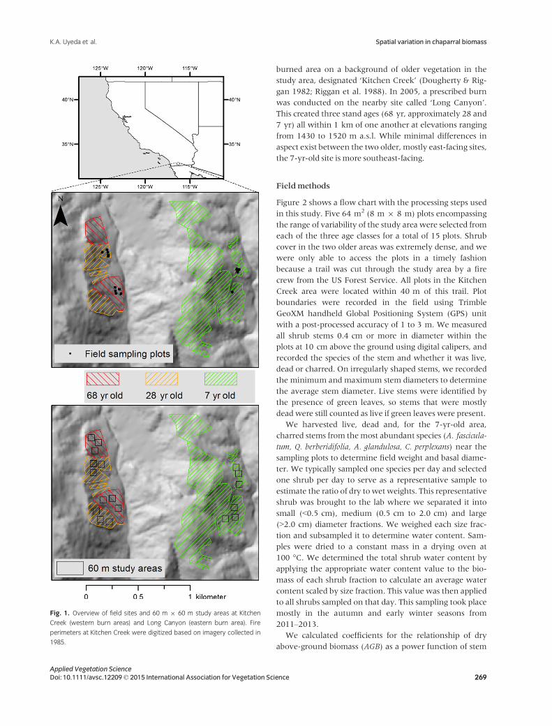
Figure 2 shows a flow chart with the processing steps used in this study. Five 64 m2 (8 m 9 8 m) plots encompassing the range of variability of the study area were selected from each of the three age classes for a total of 15 plots. Shrub cover in the two older areas was extremely dense, and we were only able to access the plots in a timely fashion because a trail was cut through the study area by a fire crew from the US Forest Service. All plots in the Kitchen Creek area were located within 40 m of this trail. Plot boundaries were recorded in the field using Trimble GeoXM handheld Global Positioning System (GPS) unit with a post-processed accuracy of 1 to 3 m. We measured all shrub stems 0.4 cm or more in diameter within the plots at 10 cm above the ground using digital calipers, and recorded the species of the stem and whether it was live, dead or charred. On irregularly shaped stems, we recorded the minimum and maximum stem diameters to determine the average stem diameter. Live stems were identified by the presence of green leaves, so stems that were mostly dead were still counted as live if green leaves were present.

We harvested live, dead and, for the 7-yr-old area, charred stems from the most abundant species (A. fascicula­tum, Q. berberidifolia, A. glandulosa, C. perplexans) near the sampling plots to determine field weight and basal diame­

ter. We typically sampled one species per day and selected one shrub per day to serve as a representative sample to estimate the ratio of dry to wet weights. This representative shrub was brought to the lab where we separated it into small (<0.5 cm), medium (0.5 cm to 2.0 cm) and large (>2.0 cm) diameter fractions. We weighed each size frac­tion and subsampled it to determine water content. Sam­

ples were dried to a constant mass in a drying oven at 100 °C. We determined the total shrub water content by applying the appropriate water content value to the bio­mass of each shrub fraction to calculate an average water content scaled by size fraction. This value was then applied to all shrubs sampled on that day. This sampling took place mostly in the autumn and early winter seasons from 2011–2013.

We calculated coefficients for the relationship of dry above-ground biomass (AGB) as a power function of stem

Applied Vegetation Science Doi: 10.1111/avsc.12209 © 2015 International Association for Vegetation Science 269

Spatial variation in chaparral biomass K.A. Uyeda et al.

Build species specific regression equations

Field -based plot

measurements (stem diameter)

Shrub harvesting

(stem diameter, biomass)

High resolution aerial imagery

Plot biomass (per species)

OBIA classification (by species groups)

Classified image

Species group biomass per

area

Divide plot biomass by classified area

Select 60 × 60 m study areas

Classified 60 × 60 m study

areas

For each species group, multiply area by

biomass per area

8 × 8 m plot biomass

Select random 8 × 8 m plots from study areas

Aggregation, percent cover, mean patch

area

Landscape metric calculation

Separate data by species

Classified 8 × 8 m

plots

Select field plots from classified

image

Classified field plots

Fig. 2. Flowchart of field and remote sensing methods.

basal area (BA) with a bias correction applied (Baskerville 1972; Sprugel 1983):

0:5 sAGB ¼ B0ðBAÞB1 e ð1Þ

where s is the residual mean square, B0 is the proportional­ity coefficient and B1 is the scaling exponent.

In order to optimize time spent in the field, we gener­ated species and age-specific equations for each species in the burned areas where they were most abundant. For example, Q. berberidifolia was only occasionally found in the 7-yr-old area, so we used the equation from the 28-yr­old area rather than generating a new equation. We also generated a generic equation for each age class using the pooled measurements across all species to provide an esti­mate for less abundant species. We calculated above­ground biomass for entirely dead shrubs that could not be identified by species using the generic dead shrub equa­tion for the appropriate burn year. Charred stems were only occasionally found in the older stands, so we esti­mated charred biomass in these areas using half the value given by the appropriate equation for dead biomass.

Image classification

In order to efficiently characterize the fuel properties of each age class, we classified imagery from the 68- and

28-yr-old age classes of chaparral using colour (RGB) aerial imagery collected by Near Earth Observation Systems (NEOS) in Jun 2012 using a 21-megapixel digital camera. The imagery was geometrically corrected using control point based warping and mosaicked using nearest neigh­bour resampling to create a single image of the entire Kitchen Creek study area. The ground sample distance (GSD) of the corrected data set was 4 cm. In addition, the normalized difference vegetation index (NDVI) from May 2012 colour infrared (CIR) imagery having a nominal 50 cm GSD was also used for the classification. NDVI is cal­culated as the difference of near infrared and red digital number values divided by the sum of those values. While some of the 7-yr-old age class was covered by the NEOS imagery, the coverage was not sufficient to classify vegeta­tion within the entire area. Thus, the 2012 50 cm CIR ima­

gery was used as input to the image classification. NEOS imagery was used as a reference for training purposes.

The image-based classification system consisted of the categories broad-leaf shrubs, Af/Ag, sub-shrub, bare and dead categories. We aggregated the biomass measured in the field to those categories. The broad-leaf category mostly consisted of Q. berberidifolia and C. perplexans, although the less common species Ceanothus leucodermis, Cercocarpus betuloides, Quercus agrifolia, Rhamnus ilicifolia, Rhus ovata, Rhus trilobata and Ribes indecorum were also

Applied Vegetation Science Doi: 10.1111/avsc.12209 © 2015 International Association for Vegetation Science 270

K.A. Uyeda et al. Spatial variation in chaparral biomass

included. The Af/Ag class included the species A. fascicula­tum and A. glandulosa. We treated these species as a sepa­rate class since they featured a lower biomass per area than the other shrub species. The sub-shrub category was mostly composed of Salvia apiana, but also included small amounts of Trichostema lanatum, Keckiella ternata, Hazardia squarrosa and Eriogonum fasciculatum. The bare category was mostly composed of granite outcroppings in the 28­and 68-yr-old areas, and a combination of granite outcrop­pings and bare ground in the 7-yr-old area. The dead cate­gory included only shrubs that were entirely dead. Dead biomass attached to living shrubs was included within the appropriate species group. We were unable to classify dead cover in the 7-yr-old area due to the relatively coarse reso­lution of the imagery and small quantity of dead material in this area. We collected calibration/validation samples from 1 m 9 1 m plots in the Kitchen Creek study area (68- and 28-yr-old vegetation) along the trail using the Trimble GeoXM GPS unit. Eighteen of the plots were used to train the classifier, and 42 were used for validation.

We used eCognition, an object-based image analysis (OBIA) software package, for image-based classification of vegetation types (eCognition Developer 8.9, http:// www.ecognition.com/). OBIA segments an image into groups of adjacent pixels (objects) and then assigns these objects to the categories of the classification scheme based on a set of user-defined rules. We used an iterative seg­mentation/classification approach, re-segmenting several times to create objects of the appropriate size for the class of interest. A multi-resolution segmentation algorithm with scale parameters of 10 and 15 was implemented, as well as the chessboard segmentation algorithm with object sizes of 1 and 10. The multi-resolution segmentation algo­rithm works by iteratively merging adjacent pixels based on criteria of spectral and shape homogeneity, and the scale parameter modifies the size of the final image objects. The chessboard segmentation algorithm simply divides the image into equally sized square objects. After each round of segmentation, we used properties such as texture, brightness, colour, adjacency and NDVI to classify the objects in the class of interest, then merged the unclassified objects so they could be re-segmented with appropriate parameters for the next class of interest. Although we made minor manual corrections to the vegetation type maps in the primary study area, the accuracy assessment was based on the uncorrected classification results.

Landscape analysis

Vegetation cover percentages of each field plot were extracted from the image classification product. We cal­culated biomass per m2 using biomass measured in the field and species category cover taken from imagery

classification. We used the average biomass per m2 of the two plots from each age and species category with the highest field measured biomass for a given species category. Since the plots were composed of a mixture of species, samples of some plots were not representa­tive of the species category of interest. In order to reduce the error associated with these plots, we based our calculation on only the plots in which the species category of interest was abundant. In order to provide a more cautious estimate of biomass, we also calculated the average biomass per m2 for the combined 68- and 28-yr-old areas. We did not include the 7-yr-old area in this calculation because these values were much lower than those found in the older burn areas.

There were not enough areas of sub-shrub in the 68-yr­old plots to calculate an average, so the values for these plots were estimated from the 28-yr-old plots. Dead bio­mass per area values fluctuate so widely that it was not possible to calculate realistic values with the procedure used for the rest of the species groups. We simply used a value of 2 kgmm -2 to approximate dead vegetation. This approximation is based on half the value calculated for the combined 68- and 28-yr-old Af/Ag coefficient.

We selected six 60 m 9 60 m study areas within each age class for a total of 18 large study areas. We selected this size because it was the largest area that would fit in the burn perimeters of the 7-yr-old area. We clustered the study areas into three northern and three southern study areas, each separated by at least 200 m (Fig. 1). The aspect of the 60 m 9 60 m study areas, based on a 10 m spatial resolution digital elevation model, is shown in Appendix S1. In each of these study areas, we randomly selected five 8 m 9 8 m plots for a total of 30 plots per burn age (90 plots total).

The landscape properties of aggregation index and patch size were derived from vegetation-class patches from the 18 large study areas using the software program Fragstats (v 4.1, http://www.umass.edu/landeco/research/fragstats/ fragstats.html). The aggregation index is calculated by dividing the cell adjacencies of a given class by the total number of possible cell adjacencies for that class. It is given as a percentage, such that a given class clumped in a single, compact patch would have a value near 100. Patch size for each species group was calculated using the area-weighted patch mean size, in which each patch is weighted by its proportional area representation. We also examined spe­cies composition by calculating the percentage cover of each species group. Since the vegetation map of the 7-yr­old age class was produced using 0.5 m imagery, we reduced the resolution of the 68- and 28-yr-old age classes (originally 4 cm) to match this lower resolution of 50 cm. In order to more closely examine the differences in the 68­and 28-yr-old age classes, we also calculated the same met-

Applied Vegetation Science Doi: 10.1111/avsc.12209 © 2015 International Association for Vegetation Science 271

Spatial variation in chaparral biomass K.A. Uyeda et al.

rics using the original resolution (4 cm) vegetation classifi­cation.

Data analysis

The first research question – how does stand-level biomass vary as a function of stand age? – was addressed using the classified map of biomass. We calculated the total biomass using the age-specific coefficients determined previously. To determine if differences in biomass were robust to possi­ble error in the age-specific coefficients, we also calculated an estimate of biomass using the averaged coefficients for the 68- and 28-yr-old age classes. We tested for biomass differences in the three age classes with one-way ANOVA (n = 30).

We addressed the second research question – how do the landscape properties of aggregation index and patch size vary in each of the dominant species groups as a func­tion of stand age? – using the landscape scale metrics from

7-yr-old 1010

the 60 m 9 60 m study areas. We compared the differ­ence in these metrics in the three age classes with one-way ANOVA (n = 6). We compared the landscape metrics for the original resolution vegetation classification based on two age classes using a series of t-tests (n = 6).

Results

Stand-level biomass

Regressions of biomass as a function of basal area for the four chaparral species are presented in Fig. 3, and regres­sion coefficients are shown in Appendix S2. The coefficient of determination (R2) values for the biomass equations ranged from 0.82 to 0.97. The R2 values for dead biomass were somewhat lower, and ranged from 0.65 to 0.96. The covariation between biomass and basal area was highest in 68-yr-old Q. berberidifolia and lowest in 7-yr-old A. fascicu­latum. We were able to use a species-specific equation to calculate shrub biomass for at least 90% of the total basal

28-yr-old 68-yr-old10

1 1 1

0.1 0.1 0.1

0.01 0.010.01

perp

lexa

ns

C.

Q. b

erbe

ridifo

lia

A. f

asci

cula

tum

glan

dulo

saA

.bi

omas

s (k

g)

0.001 0.0010.001 0.01 1 100 0.01 1 100 0.01 1 100

Basal area (cm2) Basal area (cm2) Basal area (cm2)

10

0.001

0.01

0.1

1

10

0.01 1 100 0.01 1 100

Bio

mas

s (k

g) 1

0.1

0.01

0.001

Basal area (cm2) Basal area (cm2) 1010

11

0.10.1

0.010.01

0.0010.001 0.01 1 100 0.01 1 100

Basal area (cm2)

Bio

mas

s (k

g)

Basal area (cm2)

10

0.01 1 100

Bio

mas

s (k

g) 1

0.1

0.01

0.001

Basal area (cm2)

Fig. 3. Regressions of biomass as a function of basal area. The dotted line is the 10:1 line.

Applied Vegetation Science Doi: 10.1111/avsc.12209 © 2015 International Association for Vegetation Science 272

K.A. Uyeda et al. Spatial variation in chaparral biomass

area present in each plot. We made every effort to sample shrubs from the full range of basal area values found in the field plots, but it was not always possible to locate large enough shrubs for the destructive sampling. A maximum of 4% (and usually much less) of all stems in the field plots were so large as to require an extrapolation of the regres­sion equation to estimate biomass.

Biomass measurements from the field survey ranged -2 -2from 7.5 kgmm in one of the oldest plots to 1.1 kgmm in

one of the youngest plots (Appendix S3). The highest bio­mass values were found in the 68-yr-old stand, particularly in plots dominated by Q. berberidifolia. Despite these much higher values in the oldest plots, there was considerable overlap in the total biomass values in the 68- and 28-yr­old plots. Total biomass values were much lower in the 7­yr-old plots, as expected. Charred stems were found only occasionally in the older areas, but were abundant in the 7-yr-old area. Charred stem biomass ranged from about one-third to nearly equivalent to the amount of post-fire growth in these plots, although the regression relationship for calculating charred stem biomass exhibited a high degree of scatter, meaning that actual values of charred biomass may vary substantially from what we estimated.

The percentage of dead biomass varied substantially, but was generally higher in A. fasciculatum than other species, and overall much lower in the 7-yr-old area. Since par­tially dead stems were categorized as ‘live’ if green leaves were still present, these values represent the lower bound of percentage dead biomass. Biomass from entirely dead shrubs was also highly variable and almost completely absent in the 7-yr-old area.

The image classification product of species groups was assessed to have an overall accuracy of 71% (Table 1), based on reference data from the 1 m 9 1 m field-based validation sample plots. Accuracy was higher in the more abundant categories of broad-leaf and Af/Ag, and particu­larly low in the dead biomass category.

Estimated biomass per area ranged from 6.2 kgmm -2 in the oldest age class of broad-leaf vegetation to 0.4 kgmm -2

in the youngest age class of sub-shrub vegetation (Table 2). The biomass per area coefficients provided a good approximation of the two major categories of shrub species (Af/Ag and broad-leaf) and of overall biomass (Fig. 4a–c). The predicted Af/Ag biomass values based on the mapped cover tended to yield a closer agreement with the field-measured plot biomass values, while the broad-leaf and the combined total calculations were more vari­able.

We found a significant difference in mean biomass in the three age classes when using age-specific biomass coef­ficients (F2,87 = 326, P < 0.001), and the post-hoc Tukey test revealed that all three means were significantly differ­ent (Table 3, Fig. 5). The calculated biomass values showed a clear trend of accumulation through time (Fig. 5). However, the differences between age classes were not as clear when using the biomass values calculated using pooled coefficients (average of 28- and 68-yr-old areas). Although the overall ANOVA was significant (F2,87 = 243, P < 0.001), the post-hoc Tukey test revealed that the 28- and 68-yr-old areas were not significantly dif­ferent (Table 3, Fig. 5). An overall trend of increasing bio­mass through time was evident, but when using these pooled coefficients, the difference between the 68- and 28­yr-old areas was not significant (Fig. 5). Both the results from the age-specific and pooled coefficients revealed a

Table 2. Above-ground biomass per unit area based on classification.

Veg type Age class kgmm -2

Broad-leaf 68 6.2

Broad-leaf 28 4.2

Broad-leaf 7 2.4

Broad-leaf 68/28 5.2

Af/Ag 68 4.3

Af/Ag 28 3.6

Af/Ag 7 1.4

Af/Ag 68/28 4

Sub-shrub 68/28 1.5

Sub-shrub 7 0.4

Table 1. Error matrix from field-based accuracy assessment of the classified high spatial resolution map.

Field classification

Af/Ag Bare Broad-leaf Dead Sub-shrub Total User accuracy

Remote sensing classification Af/Ag 10 1 4 0 0 15 0.67

Bare 0 2 0 0 1 3 0.67

Broad-leaf 3 0 17 2 0 22 0.77

Dead 1 0 0 0 0 1 0.00

Sub-shrub 0 0 0 0 1 1 1.00

Total 14 3 21 2 2 42

Producer accuracy 0.71 0.67 0.81 0.00 0.50 Overall accuracy

0.71

Applied Vegetation Science Doi: 10.1111/avsc.12209 © 2015 International Association for Vegetation Science 273

Spatial variation in chaparral biomass K.A. Uyeda et al.

668 yr 28 yr 7 yr

5400

4

Tota

l bio

mas

s (k

g·m

–2)

7 yr 28 yr 68 yr

a

b

c

a

b b

Age 3 specific

Map

-est

imat

ed b

iom

ass

(kg)

M

ap-e

stim

ated

bio

mas

s (k

g)

Map

-est

imat

ed b

iom

ass

(kg) Af/Ag(a)

0 100 200 300 400

300

200

100

2 Pooled

1

0 0

Field-estimated biomass (kg) Stand age

400

300 post-hoc Tukey tests. Bars with different letters are significantly different

(P < 0.05)

200

wide range in biomass values for each stand age calculated 100 for the 30 sampling plots (Table 3).

0 Landscape properties

Field-estimated biomass (kg) The general trend of average percentage cover in the

Broadleaf(b)

0 100 200 300 400

Fig. 5. Total biomass means using age-specific biomass coefficients and

pooled biomass coefficients. Error bars indicate SE and letters indicate

400 Total biomass(c)

0 100 200 300 400

300

200

100

0

Field-estimated biomass (kg)

60 m 9 60 m study areas within each burn area indicates that broad-leaf percentage cover was higher in the older areas, sub-shrub cover was lower, and bare was not differ­ent (Fig. 6). Af/Ag cover was higher in the 28- than 7-yr­old area, and was similar in the 28- and 68-yr-old areas. However, closer inspection of the associated ANOVA results indicated that while there was a significant cover difference among several of the vegetation classes in each age class (e.g. broad-leaf, F2,15 = 10.2, P = 0.0016), post-hoc Tukey tests revealed that only the youngest age class was significantly different from the two older age classes

Fig. 4. Field-estimated biomass vs biomass estimated using age-specific

biomass coefficients in each field plot for (a) Af/Ag, (b) broad-leaf, and (c)

total biomass. The dotted line is the 1:1 line.

Table 3. Mean, range and ANOVA results for stand-level biomass com­

parisons using age-specific and pooled biomass coefficients. df = 2,87,

n = 30

7 yr 28 yr 68 yr F P

Age-specific

1.3 3.4 5.1 326 <0.001

Mean (kgmm -2)

range 0.5–2.2 1.6–4.0 3.8–6.0

Pooled

1.3 4.0 4.4 243 <0.001

Mean (kgmm -2)

range 0.5–2.2 1.9–4.9 3.5–5.1

(Table 4, Fig. 7a). The post-hoc Tukey tests showed the same pattern for the Af/Ag category and in the sub-shrub category, only the youngest and oldest age classes were sig­nificantly different (Fig. 7a).

In general across stand ages, the aggregation index (landscape pattern metric) is higher (more aggregated) in the broad-leaf and Af/Ag classes, and lower (more dis­persed) for the sub-shrub and bare categories. Within the three age classes, only in the Af/Ag and sub-shrub cate­gories are there significant differences in aggregation index with age (Af/Ag F2,15 = 6.8, P = 0.0079, sub-shrub F2,15 = 6.9, P = 0.0077; Table 4). Post-hoc Tukey tests show that in the Af/Ag category, only the 7- and 28-yr-old age classes are significantly different from one another, and in the sub-shrub category, only the 7- and 68-yr-old age classes are significantly different (Fig. 7b).

Area-weighted patch mean area is higher for the older age classes in the broad-leaf category, with only the differ-

Applied Vegetation Science Doi: 10.1111/avsc.12209 © 2015 International Association for Vegetation Science 274

K.A. Uyeda et al. Spatial variation in chaparral biomass

Ave

rage

cov

er (%

)

100

Dead 80

Bare 60

Subshrub

40 Af/Ag

20 Broadleaf

0 7 yr 28 yr 68 yr

Fig. 6. Average percentage cover in the three age classes. Note that

dead cover could not be estimated in the 7-yr-old age class.

ence between the youngest and oldest age class being sig­nificant (F2,15 = 8.0, P = 0.0042; Table 4). Patch mean area was lower in the youngest age class in the Af/Ag cate­gory, and the youngest area is significantly different than the two older areas (F2,15 = 15.8, P = 0.0002; Fig. 7c).

The series of t-tests of landscape metrics generated from the higher resolution (4 cm) classified imagery comparing the two older age classes indicate that the only significantly different classification/landscape metric combination is percentage cover of sub-shrub, which is higher for the 28­yr-old area (df = 9.561, P = 0.009; Table 5).

Discussion

Stand-level biomass

We could not make statistical inferences regarding the overall stand composition based on the field data. This was due to the sampling of plots that represented the range of variability found in our study area rather than random plots. We instead presented general observations about the

species composition and overall biomass present in the field plots. For this reason, we did not present averages or estimates of error associated with plot biomass values.

We found a high degree of variability in biomass in the study area due to species composition and stand age. Older stands had higher levels of biomass per area, and coeffi­cients of the tall, dense species that make up the broad-leaf category were highest, followed by the more sparse Af/Ag category species, and finally by the much smaller sub-shrub species category. The regression equations calculated in this study were similar to those calculated in a previous study of the same area for the corresponding species and age (Riggan et al. 1988). The resulting biomass per area values were higher for each age than found by Riggan et al. (1988), but similar to those found in other studies within southern California (Black 1987; Riggan et al. 1988). Although the exact biomass per area coefficient val­ues is not necessarily applicable to areas outside of this field site, these values provide valuable field data to more accu­rately map and estimate stand-level biomass across the study area. The high spatial resolution of the mapping effort allowed non-shrub cover (such as large rock out­crops) to be efficiently removed from the estimates of bio­mass per area. This means that caution must be used when applying the biomass coefficients from this study to map­

ping efforts based on lower resolution imagery, in which rock outcrops might not be reliably separated from shrub cover. Field-based biomass sampling is often too time con­suming and logistically difficult to be conducted over large study areas (Lu 2006). Using remotely sensed imagery allows for biomass estimation over of much larger areas in an efficient manner. Our approach of using high spatial resolution imagery with object-based methods is reason­ably successful for mapping fine-scale variation in species composition. Considering all the potential sources of error and uncertainty due to geolocation accuracy, field mea­

surement error and other possible sources, it is promising

Table 4. ANOVA results for class metrics for the classified standardized resolution (0.5 m) data set. Bold P-values indicate significant results (P ≤ 0.01).

df = 2,15, n = 6.

Class Metric Mean 7-yr-old Mean 28-yr-old Mean 68-yr-old F P

Broad-leaf Aggregation 83 86 89 3.0 0.0816

Af/Ag Aggregation 81 65 70 6.8 0.0079

Sub-shrub Aggregation 53 39 31 6.9 0.0077

Bare Aggregation 44 63 53 3.8 0.0477

Broad-leaf % of landscape 26 60 67 10.2 0.0016

Af/Ag % of landscape 51 19 19 13.9 0.0004

Sub-shrub % of landscape 17 6 3 6.7 0.0083

Bare % of landscape 6 7 5 0.9 0.4315

Broad-leaf Mean patch area (m2) 321 1514 2155 8.0 0.0042

Af/Ag Mean patch area (m2) 1293 173 127 15.8 0.0002

Sub-shrub Mean patch area (m2) 79 5 3 4.1 0.0378

Bare Mean patch area (m2) 6 20 10 1.8 0.2059

Applied Vegetation Science Doi: 10.1111/avsc.12209 © 2015 International Association for Vegetation Science 275

Spatial variation in chaparral biomass K.A. Uyeda et al.

could likely be further improved by using high spatial reso-Subshrub Af/Ag Broadleaf lution colour infrared imagery. 100

a

(a)

a

a b

ab

b

b

b

b

It is more challenging to derive reliable maps of dead biomass based on image-based classification. This is partly due to the tendency of dead biomass to be located beneath plant canopies composed mostly of live biomass, either as dead stems within a single shrub or as an entirely dead

Agg

rega

tion

inde

x P

erce

ntag

e of

tota

l are

a

75

50 shrub surrounded by live shrubs. This means that although dead biomass is often spread uniformly throughout stands of chaparral, it is only occasionally visible from above (which would allow it to be measured through aerial ima­

gery). These small patches of dead biomass are not repre­sentative of the total dead biomass found in an area and

25

0 make it more difficult to derive a relationship for biomass 7 yr 28 yr 68 yr per unit area.

We calculated stand-level biomass in two ways to pro­100

75

50

25

a

a

(b)

b

ab

ab

b

vide a more cautious estimate for the older sites. While results for the age-specific coefficients show a substantially higher biomass for the 68-yr-old areas, the results from the pooled coefficients indicate that the difference is not statis­tically significant. It is possible that if the 68-yr-old area had substantially more broad-leaf cover than the 28-yr-old area, the broad-leaf coefficient (higher than the Af/Ag coefficient in both the age-specific and pooled calculations) might have resulted in a higher biomass value in both cal­culations. However, it appears that differences are not that dramatic. Regardless of whether biomass continues to accumulate, it is clear that biomass levels remained high in the oldest stand of chaparral, consistent with the findings of previous studies (Specht 1969; Black 1987). Unsurpris­

0 7 yr 28 yr 68 yr

3000

a

a

(c)

ab

b

b

b

ingly, there was a large difference in biomass between the 7-yr-old and 28-yr-old stands. Shrub growth is rapid dur­ing this early phase of post-fire recovery and shrubs quickly expand in both cover and stature (Rundel & Par­sons 1979; Keeley & Keeley 1981). While there were site

Mea

n pa

tch

area

(m2 ) 2500

2000

1500 differences between the 7-yr-old site and the older sites, the measurements of biomass per unit area for each species

1000 were based on areas in which each species is dominant.

Although it is still uncertain whether or not biomass continues to appreciably accumulate at older stand ages,

500

0 7 yr 28 yr 68 yr

Fig. 7. (a–c) Mean and SE of significantly different age classes for the: (a)

percentage of total area for sub-shrub, Af/Ag and broad-leaf categories, (b)

aggregation index for Af/Ag and broad-leaf categories, and (c) mean patch

area for Af/Ag and broad-leaf categories from the standardized resolution

(0.5 m) data set. Letters indicate post-hoc Tukey comparisons. Bars with

different letters are significantly different (P ≤ 0.05).

that coefficients based on just two plots per stand age and species category yield such close agreement between field-estimated and map-estimated biomass. Mapping success at the species category level (and by extension, biomass)

the high number of plots examined through the scaling approach revealed a wide range of biomass values within a single age class. It is noteworthy that biomass varied so widely at the plot level (8 m 9 8 m) within a relatively constrained spatial extent in an even-aged stand. This fine-scale spatial variation is typically difficult to map and might be important in understanding fire behaviour (Keane et al. 2001).

The scaling approach used in this study is based on two separate relationships, which has advantages and disad­vantages. The final biomass values depend on both the stem-to-biomass regression relationship and the field-mea­

sured biomass-to-mapped cover category relationship. The

Applied Vegetation Science Doi: 10.1111/avsc.12209 © 2015 International Association for Vegetation Science 276

K.A. Uyeda et al. Spatial variation in chaparral biomass

Table 5. t-test results from comparison of class metrics for classification of original resolution (4 cm) imagery from 68- and 28 yr-old sites. Bold P-value

indicates significant results (P ≤ 0.01). n = 6.

Class Metric Mean 28-yr-old Mean 68-yr-old df P

Broad-leaf Aggregation 98 99 6.091 0.419

Af/Ag Aggregation 95 96 10.000 0.266

Sub-shrub Aggregation 88 87 9.505 0.697

Bare Aggregation 95 93 6.670 0.182

Dead Aggregation 88 89 9.992 0.935

Broad-leaf % of landscape 60 68 7.255 0.389

Af/Ag % of landscape 19 19 9.783 0.982

Sub-shrub % of landscape 6 3 9.561 0.009

Bare % of landscape 7 5 9.930 0.084

Dead % of landscape 8 6 9.108 0.228

Broad-leaf Mean patch area (m2) 1477 2105 9.850 0.269

Af/Ag Mean patch area (m2) 168 147 8.814 0.910

Sub-shrub Mean patch area (m2) 4 5 6.338 0.922

Bare Mean patch area (m2) 19 10 7.250 0.297

Dead Mean patch area (m2) 3 3 9.848 0.852

benefit of this approach is that it allowed for estimates over a much larger study area than could be adequately achieved using field sampling alone. However, there is an increased potential for error to propagate through the cal­culations. Still, the high degree of fine-scale variation observed in this study indicates that it was worthwhile to extrapolate the results across a larger area through this scaling approach at the cost of some degree of accuracy.

Landscape properties

Although landscape properties between the 28- and 68-yr­old areas are not substantially different, several signifi­cantly different relations were identified between the 7-yr­old site and the older sites. Broad-leaf cover and patch size were larger, while Af/Ag cover and patch size were smaller in the older age classes. Sub-shrub cover was also lower in the older age classes. While some of these differences might be due to age, it was difficult to make definitive comparisons in landscape properties between the 7-yr-old site and the older sites due to the slightly different aspect of the younger stand (more southeast-facing, compared to the more directly east-facing older sites). Another potential issue with these landscape-level comparisons was that the original classification of the youngest age site was based on a different (and lower resolution) imagery source than the older age classes. While we reduced the spatial resolution of the older age classes to make the results more compara­

ble, it is possible that the results would be different had we been able to use high spatial resolution imagery for the entire study area. In particular, we likely would have been able to more accurately classify the small (but abundant) patches of bare ground observed during our field sampling in the youngest age class. The minimum spatial resolution required to detect a given feature on the ground is

generally considered to be one-half the diameter of that feature (Jensen 2005), and many bare patches observed in the field were smaller than 1 m in diameter. However, the overall trends we observed through the analysis of image-

derived landscape properties seem consistent with obser­vations in the field.

It is also important that almost no significant differences in the landscape properties of the 28- and 68-yr-old stands were identified, even when the high spatial resolution classi­fication results were compared. Other than a small differ­ence in sub-shrub cover, there were no differences in aggregation, percentage of landscape or patch size in these two older age classes. Although we were unable to confi­dently relate field measurements of dead biomass to classi­fied dead biomass cover, it is still noteworthy that there was no significant difference in the landscape-level properties of dead biomass in the two older age classes. A high level of dead biomass in the oldest stand could indicate age-related die back, as observed by Hanes (1971). However, we observed no such age-related shrub die back in the older age classes, consistent with the findings of Keeley (1992).

Conclusion

While it is unclear whether there was a net accumulation in stand biomass from the age of 28 to 68 yr, there was lit­tle difference in the spatial arrangement of species groups in the two age groups. Biomass per unit area for each spe­cies was much lower in the 7-yr-old stand compared to the two older stands, and it seems reasonable to expect that for a given species, the trend towards higher biomass with increasing age reflects the process of post-fire shrub recov­ery. Due to the difference in aspect in the youngest stand, it was more difficult to determine if the differences in total biomass and landscape properties represented an age-

Applied Vegetation Science Doi: 10.1111/avsc.12209 © 2015 International Association for Vegetation Science 277

Spatial variation in chaparral biomass K.A. Uyeda et al.

related trend. In all age classes, we found a wide range of biomass values, indicating a high degree of spatial variabil­ity within chaparral. It was difficult to map dead biomass, although simply knowing the species distribution could help inform estimates of dead biomass, as A. fasciculatum is known to retain dead stems (Schwilk 2003). Dead fuel loading is a significant attribute for modelling fire beha­viour, so improved mapping of dead biomass is an impor­

tant area for future research. Although our field sampling was somewhat limited due

to the physically difficult and time consuming nature of the measurements in barely penetrable mature chaparral shrublands, we were able to extrapolate our field sample across the entire study area through the use of high spatial resolution imagery and OBIA classification of vegetation types. Our approach of combining detailed field measure­

ments with remotely sensed classification of dominant spe­cies groups to map the spatial arrangement of fuels in chaparral is a valuable method for characterizing biomass accumulation. An increased understanding of patterns of biomass accumulation could improve the accuracy of fuel mapping, which is important to fire management. Fuel maps are used for many purposes before and during wild­

fires, including planning fuel reduction treatments and modelling fire behaviour. Fire behaviour modelling relies on coarse-scale fuel models that do not take into account biomass accumulation through time or the wide range in biomass often present within a single stand (Riggan et al. 2010). Understanding biomass accumulation over a wide range of temporal and spatial scales could help to improve the inputs to fire behaviour models, increasing the accu­racy of the predicted behaviour.

Acknowledgements

We thank J. Truett, T. Hayes and J. Kraling from the USFS for arranging for site access. We also thank D. Rachels, C. Riggan, A. Brown, F. Uyeda, J. Jesu, B. Lo, B. Corcoran, D. Smith and Y. Granovskaya for assistance in the field. Fund­ing for this project was provided by the USDA Forest Ser­vice through American Recovery and Reinvestment Act Agreement No. 10-JV-11279701-10: Airborne remote sensing to enable hazardous fuels reduction, forest health protection, rehabilitation and hazard mitigation activities on federal lands.

References

Arroyo, L., Pascual, C. & Manzanera, J. 2008. Fire models and

methods to map fuel types: the role of remote sensing. Forest

Ecology and Management 256: 1239–1252.

Baldwin, B.G., Goldman, D.H., Keil, D.J., Patterson, R.,

Rosatti, T.J. & Wilken, D.H. 2012. The Jepson manual: vas­

cular plants of California. University of California Press,

Berkeley, CA, US.

Baskerville, G. 1972. Use of logarithmic regression in the estima­

tion of plant biomass. Canadian Journal of Forest Research 2:

49–53.

Black, C.H. 1987. Biomass, nitrogen, and phosphorus accu­

mulation over a southern California fire cycle chronose­

quence. In: Tenhunen, J.D., Catarino, F.M., Lange, O.L.

& Oechel, W.C. (eds.) Plant response to stress – functional

analysis in mediterranean ecosystems, pp. 445–458. Springer,

Berlin, DE.

Countryman, C.M. & Dean, W.A. 1979. Measuring moisture con­

tent in living chaparral: a field user’s manual. Berkeley, CA,

Gen. Tech. Rep. PSW-36. USDA Forest Service. Pacific

Southwest Forest and Range Experiment Station, Forest Ser­

vice, U.S. Department of Agriculture, 1982, Berkeley, CA,

US.

Countryman, C.M. & Philpot, C.W. 1970. Physical characteristics of

chamise as a wildland fuel. Research Paper PSW- 66, Pacific

Southwest Forest & Range Experiment Station, Forest Ser­

vice, U.S. Department of Agriculture, Berkeley, CA, US.

Davis, S., Ewers, F., Sperry, J., Portwood, K.A., Crocker, M.C. &

Adams, G.C. 2002. Shoot dieback during prolonged drought

in Ceanothus (Rhamnaceae) chaparral of California: a possi­

ble case of hydraulic failure. American Journal of Botany 89:

820–828.

Dougherty, R. & Riggan, P.J. 1982. Operational use of prescribed

fire in Southern California chaparral. In: Conrad, C.E. &

Oechel, W.C. (eds.), Proceedings of the symposium on dynamics

and management of Mediterranean-type ecosystems, pp. 502–510,

Gen. Tech. Rep PSW-58, Pacific Southwest Forest and Range

Experiment Station, Forest Service, U.S. Department of Agri­

culture, Berkeley, CA, US.

Green, L.R. 1970. An experimental prescribed burn to reduce fuel haz­

ard in chaparral. USDA Forest Service Research Note PSW­

216, Berkeley, CA, US.

Hanes, T.L. 1971. Succession after fire in the chaparral of south­

ern California. Ecological Monographs 41: 27–52.

Hiers, J.K., O’Brien, J.J., Mitchell, R.J., Grego, J.M. & Louder-

milk, E.L. 2009. The wildland fuel cell concept: an approach

to characterize fine-scale variation in fuels and fire in fre­

quently burned longleaf pine forests. International Journal of

Wildland Fire 18: 315.

Jensen, J.R. 2005. Introductory digital image processing: a remote

sensing perspective. Pearson Prentice Hall, Upper Saddle River,

NJ, US.

Keane, R.E., Burgan, R. & van Wagtendonk, J. 2001. Mapping

wildland fuels for fire management across multiple scales:

integrating remote sensing, GIS, and biophysical modeling.

International Journal of Wildland Fire 10: 301–319.

Keeley, J.E. 1992. Demographic structure of California chaparral

in the long-term absence of fire. Journal of Vegetation Science

3: 79–90.

Keeley, J.E. & Keeley, S.C. 1981. Post-fire regeneration of south­

ern California chaparral. American Journal of Botany 68: 524.

Applied Vegetation Science Doi: 10.1111/avsc.12209 © 2015 International Association for Vegetation Science 278

K.A. Uyeda et al.

Keeley, J.E. & Zedler, P.H. 2009. Large, high-intensity fire events

in southern California shrublands: debunking the fine-grain

age patch model. Ecological Applications 19: 69–94.

Keeley, S.C., Keeley, J.E., Hutchinson, S. & Johnson, A. 1981.

Postfire succession of the herbaceous flora in southern Cali­

fornia chaparral. Ecology 62: 1608–1621.

Lu, D. 2006. The potential and challenge of remote sensing based

biomass estimation. International Journal of Remote Sensing 27:

1297–1328.

Mahall, B.E. & Wilson, C.S. 1986. Environmental induction and

physiological consequences of natural pruning in the cha­

parral shrub Ceanothus megacarpus. Botanical Gazette 147: 102–

109.

McMichael, C.E., Hope, A.S., Roberts, D.A. & Anaya, M.R. 2004.

Post-fire recovery of leaf area index in California chaparral: a

remote sensing-chronosequence approach. International

Journal of Remote Sensing 25: 4743–4760.

Moritz, M.A., Keeley, J.E., Johnson, E.A. & Schaffner, A.A.

2004. Testing a basic assumption of shrubland fire manage­

ment: how important is fuel age? Frontiers in Ecology and the

Environment 2: 67–72.

Paysen, T.E. & Cohen, J.D. 1990. Chamise chaparral dead fuel

fraction is not reliably predicted by age. Western Journal of

Applied Forestry 5: 127–131.

Regelbrugge, J.C. & Conard, S.G. 1996. Biomass and fuel charac­

teristics of chaparral in southern California. 13th Conference

on Fire and Forest Meteorology.

Riggan, P.J., Goode, S., Jacks, P.M. & Lockwood, R.N. 1988.

Interaction of fire and community development in

chaparral of Southern california. Ecological Monographs 58:

156–176.

Riggan, P.J., Franklin, S., Brass, J. & Brooks, F. 1994. Perspec­

tives on fire management in Mediterranean ecosystems of

southern California. In: Moreno, J.M. & Oechel, W.C. (eds.)

The role of fire in Mediterranean-type ecosystems, pp. 140–162.

Springer, New York, NY, US.

Riggan, P.J., Wolden, L.G., Tissell, R.G., Weise, D.R. & Coen, J.L.

2010. Remote sensing fire and fuels in Southern California.

In: Wade, D.D. & Robinson, M.L. (eds) Proceedings of 3rd

Fire Behavior and Fuels Conference, October 25–29, 2010,

Spatial variation in chaparral biomass

Spokane, Washington, USA, pp. 1–14. International Associa­

tion of Wildland Fire, Birmingham, AL, US.

Rundel, P.W. & Parsons, D.J. 1979. Structural changes in cha­

mise (Adenostoma fasciculatum) along a fire-induced age gradi­

ent. Journal of Range Management 32: 462–466.

Schlesinger, W.H., Gray, J.T., Gill, D.S. & Mahall, B.E. 1982.

Ceanothus megacarpus chaparral: a synthesis of ecosystem pro­

cesses during development and annual growth. Botanical

Review 48: 71–117.

Schwilk, D.W. 2003. Flammability is a niche construction trait:

canopy architecture affects fire intensity. The American Natu­

ralist 162: 725–733.

Specht, R. 1969. A comparison of the sclerophyllous vegetation

characteristic of mediterranean type climates in France, Cali­

fornia, and southern Australia. II. Dry matter, energy, and

nutrient accumulation. Australian Journal of Botany 17: 293–

308.

Sprugel, D. 1983. Correcting for bias in log-transformed allomet­

ric equations. Ecology 64: 209–210.

Weise, D.R., Zhou, X., Sun, L. & Mahalingam, S. 2005. Fire

spread in chaparral — “go or no-go ?”. International Journal of

Wildland Fire 14: 99–106.

Supporting Information

Additional Supporting Information may be found in the online version of this article:

Appendix S1. Map of aspect within each of the 60 m 9 60 m study areas and 8 m 9 8 m field plots, gen­erated using a 10-m spatial resolution digital elevation model. Appendix S2. Regression coefficients of stem above­ground biomass (AGB) in kilograms as a function of basal area (BA) in cm2 for each species and stand age. Appendix S3. Plot coordinates, area as measured by GPS coordinates, total plot biomass (excludes charred stem esti­mates) and total biomass per area for each plot age.

Applied Vegetation Science Doi: 10.1111/avsc.12209 © 2015 International Association for Vegetation Science 279