Spatial Variation in Higher Education Financing and the Supply of

College Graduates

John Kennan∗

University of Wisconsin-Madison and NBER

August, 2018

Abstract

In the U.S. there are large differences across States in the extent to which college education is

subsidized, and there are also large differences across States in the proportion of college graduates

in the labor force. State subsidies are apparently motivated in part by the perceived benefits of

having a more educated workforce. The paper extends the migration model of Kennan and Walker

(2011) to analyze how geographical variation in college education subsidies affects the migration

decisions of college graduates. The model is estimated using NLSY data, and used to quantify

the sensitivity of migration and college enrollment decisions to differences in expected net lifetime

income, focusing on how cross-State differences in public college financing affect the educational

composition of the labor force. The main finding is that these differences have substantial effects

on college enrollment, and that these effects are not dissipated through migration.

1 Introduction

There are substantial differences in subsidies for higher education across States in the U.S. Are these

differences related to the proportion of college graduates in each State? If so, why? Do the subsidies

change decisions about whether or where to go to college? If State subsidies induce more people to

get college degrees, to what extent does this additional human capital tend to remain in the State

that provided the subsidy?

There is a considerable amount of previous work on these issues, discussed in Section 3 below.

What is distinctive in this paper is that migration is explicitly modeled. Recent work on migration

has emphasized that migration involves a sequence of reversible decisions that respond to migration

∗Department of Economics, University of Wisconsin, 1180 Observatory Drive, Madison, WI 53706; jken-nan@ssc.wisc.edu. Earlier versions of this paper had a different title: “Higher Education Subsidies and Human CapitalMobility.” I thank Gadi Barlevy, John Bound, Rebecca Diamond, Eric French, Chao Fu, Ahu Gemici, Grey Gordon,Joseph Han, Jim Heckman, Tom Holmes, Lisa Kahn, Maurizio Mazzocco, Bob Miller, Derek Neal, Luigi Pistaferri, JackPorter, Mike Rothschild, Jean-Marc Robin, Chris Taber, Sarah Turner, Jim Walker, Yoram Weiss and many seminarparticipants for helpful comments. I thank four referees and the Editor for detailed and constructive comments on bothsubstance and exposition.

1

incentives in the face of potentially large migration costs.1 The results of Kennan and Walker (2011)

indicate that labor supply responds quite strongly to geographical wage differentials and location

match effects, in a life-cycle model of expected income maximization.

This suggests that variation in tuition rates across States should have substantial effects on

schooling decisions. This paper considers these effects in a dynamic programming model that allows

for migration both before and after acquiring a college degree. In the absence of moving costs, the

optimal policy for someone who decides to go to college is to move to the location that provides the

cheapest education (or the best value for money), and subsequently move to the labor market that

pays the highest wage. At the other extreme, if moving costs are very high, the economic incentive

to go to college depends only on the local wage premium for college graduates, and estimates based

on the idea of a national labor market are likely to be misleading. Thus it is natural to consider

college choices and migration jointly in a model that allows for geographical variation in both the

costs and benefits of a college degree.

The model is estimated using panel data from the National Longitudinal Survey of Youth (1979

Cohort); the estimation sample includes white males with at least a high school education born

between 1958 and 1964, observed annually from 1979 to 1994. College graduation is modeled as the

outcome of a stochastic process, rather than as a choice: high school graduates choose whether to

enroll in college, knowing that they may or may not emerge as college graduates, with probabilities

that depend on their ability, and on the type of college. Enrollment and migration choices are

affected by cross-State differences in college tuition and expenditures on higher education, and also

by spatial wage differences. The main empirical finding is that cross-State differences in higher

education expenditures, and (especially) in tuition levels, have substantial and long-lasting effects

on the proportion of college-educated workers in each State.

2 Geographical Distribution of College Graduates

There are big differences across States in the proportion of college graduates among those born in

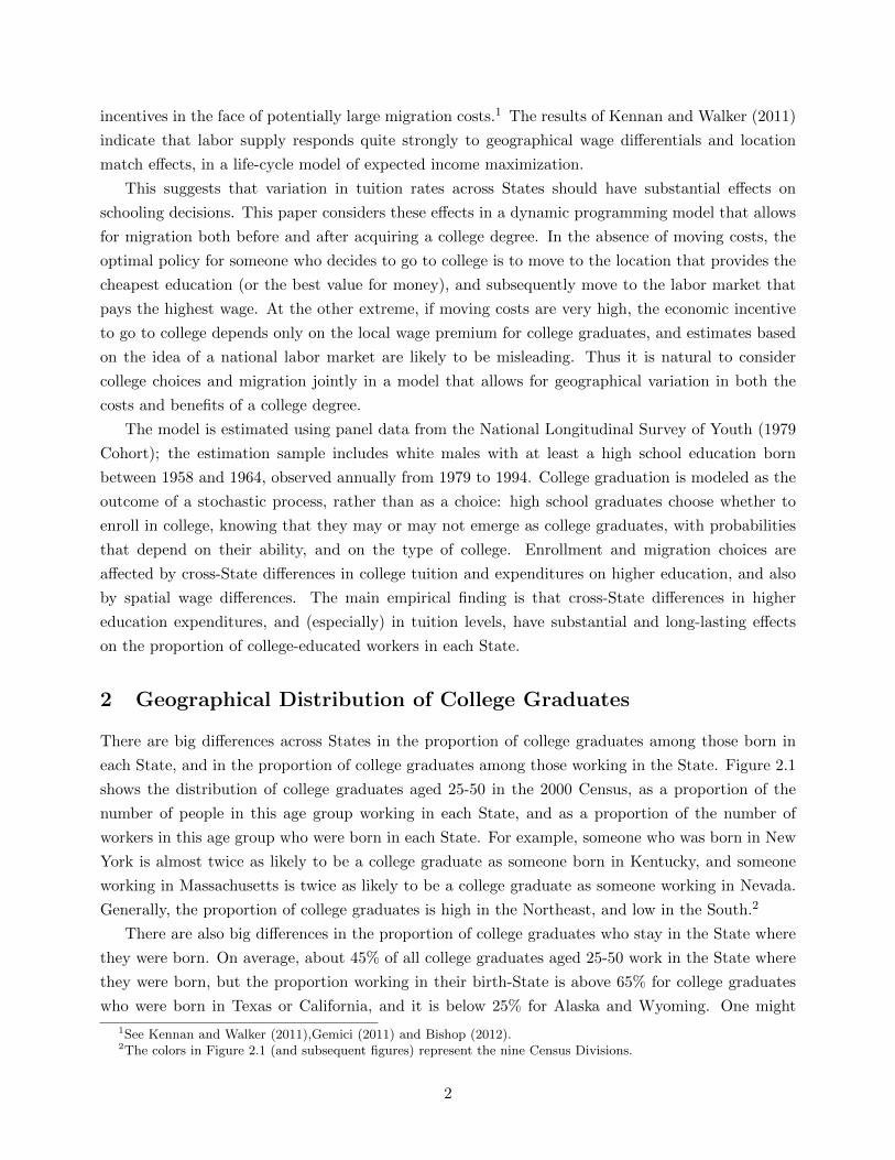
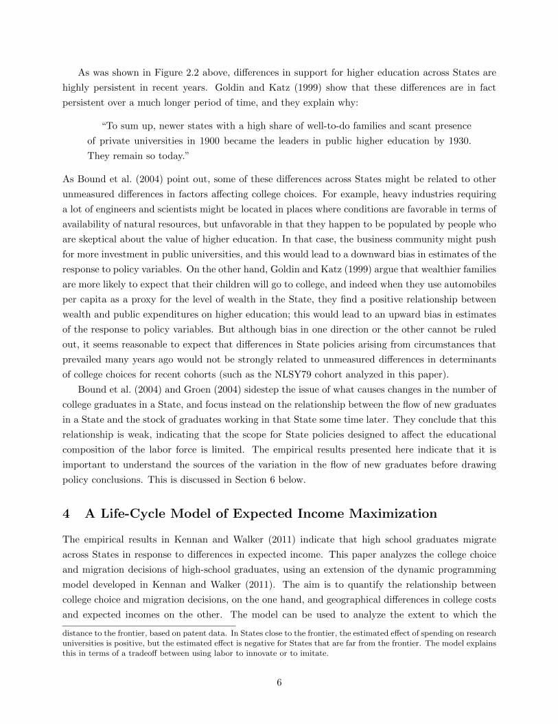
each State, and in the proportion of college graduates among those working in the State. Figure 2.1

shows the distribution of college graduates aged 25-50 in the 2000 Census, as a proportion of the

number of people in this age group working in each State, and as a proportion of the number of

workers in this age group who were born in each State. For example, someone who was born in New

York is almost twice as likely to be a college graduate as someone born in Kentucky, and someone

working in Massachusetts is twice as likely to be a college graduate as someone working in Nevada.

Generally, the proportion of college graduates is high in the Northeast, and low in the South.2

There are also big differences in the proportion of college graduates who stay in the State where

they were born. On average, about 45% of all college graduates aged 25-50 work in the State where

they were born, but the proportion working in their birth-State is above 65% for college graduates

who were born in Texas or California, and it is below 25% for Alaska and Wyoming. One might

1See Kennan and Walker (2011),Gemici (2011) and Bishop (2012).2The colors in Figure 2.1 (and subsequent figures) represent the nine Census Divisions.

2

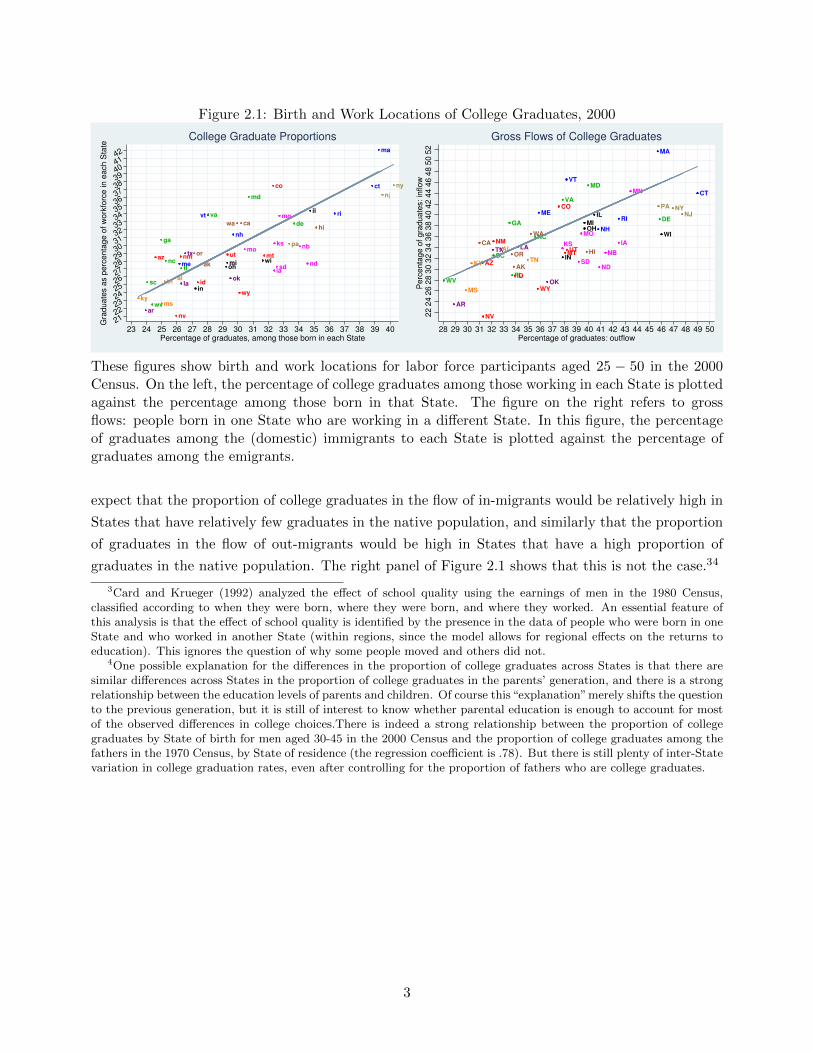
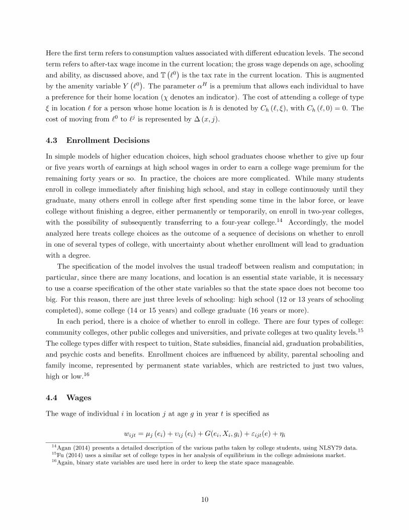
Figure 2.1: Birth and Work Locations of College Graduates, 2000

ct

me

ma

nh

rivt

nj

ny

pa

il

in

mioh

wi

ia

ks

mn

monb

ndsd

de

fl

ga

md

nc

sc

va

wv

al

kyms

tn

ar

laok

txaz

co

id

mt

nv

nm ut

wy

ak

cahi

or

wa

21222324252627282930313233343536373839404142

Gra

duate

s a

s p

erc

enta

ge o

f w

ork

forc

e in e

ach S

tate

23 24 25 26 27 28 29 30 31 32 33 34 35 36 37 38 39 40Percentage of graduates, among those born in each State

College Graduate Proportions

CT

ME

MA

NH

RI

VT

NJ

NYPA

IL

IN

MIOH

WI

IAKS

MN

MO

NB

NDSD

DE

FL

GA

MD

NC

SC

VA

WV

AL

KY

MS

TN

AR

LA

OK

TX

AZ

CO

ID

MT

NV

NM

UT

WY

AK

CA

HIOR

WA

22

24

26

28

30

32

34

36

38

40

42

44

46

48

50

52

Perc

enta

ge o

f gra

duate

s: in

flow

28 29 30 31 32 33 34 35 36 37 38 39 40 41 42 43 44 45 46 47 48 49 50Percentage of graduates: outflow

Gross Flows of College Graduates

These figures show birth and work locations for labor force participants aged 25 − 50 in the 2000Census. On the left, the percentage of college graduates among those working in each State is plottedagainst the percentage among those born in that State. The figure on the right refers to grossflows: people born in one State who are working in a different State. In this figure, the percentageof graduates among the (domestic) immigrants to each State is plotted against the percentage ofgraduates among the emigrants.

expect that the proportion of college graduates in the flow of in-migrants would be relatively high in

States that have relatively few graduates in the native population, and similarly that the proportion

of graduates in the flow of out-migrants would be high in States that have a high proportion of

graduates in the native population. The right panel of Figure 2.1 shows that this is not the case.34

3Card and Krueger (1992) analyzed the effect of school quality using the earnings of men in the 1980 Census,classified according to when they were born, where they were born, and where they worked. An essential feature ofthis analysis is that the effect of school quality is identified by the presence in the data of people who were born in oneState and who worked in another State (within regions, since the model allows for regional effects on the returns toeducation). This ignores the question of why some people moved and others did not.

4One possible explanation for the differences in the proportion of college graduates across States is that there aresimilar differences across States in the proportion of college graduates in the parents’ generation, and there is a strongrelationship between the education levels of parents and children. Of course this“explanation”merely shifts the questionto the previous generation, but it is still of interest to know whether parental education is enough to account for mostof the observed differences in college choices.There is indeed a strong relationship between the proportion of collegegraduates by State of birth for men aged 30-45 in the 2000 Census and the proportion of college graduates among thefathers in the 1970 Census, by State of residence (the regression coefficient is .78). But there is still plenty of inter-Statevariation in college graduation rates, even after controlling for the proportion of fathers who are college graduates.

3

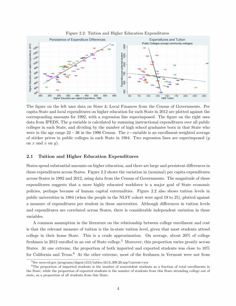
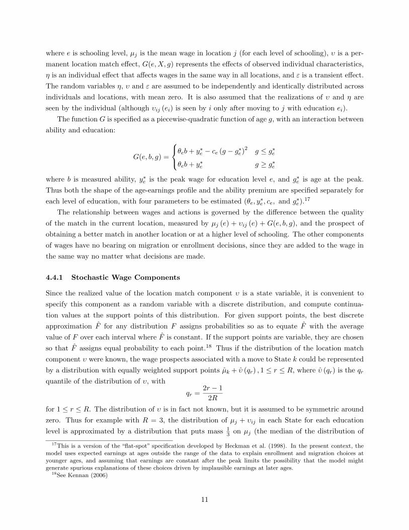
Figure 2.2: Tuition and Higher Education Expenditures

ct

me

ma

nh

ri

vt

nj

ny pail

in

mi

oh

wi

ia

ks

mn

mo

nb

nd

sd

de

fl

ga

mdnc

sc

vawv

al

kyms

tn

ar

la

oktx

az

co

id

mt

nv

nm

utwy

ak

ca

hi

or

wa

400

500

600

700

800

900

1000

1100

1200

1300

Hig

her

Education p

er

capita E

xpenditure

, 2012

200 250 300 350 400 450 500 550 600Higher Education per capita Expenditure, 1992

Persistence of Expenditure Differences

ct

me

ma

nh

ri

vt

njnypail

inmi

oh

wi

ia

ks

mn

mo

nb

nd

sd

de

flga

md

ncsc

va

wv

alky

mstn

ar

la

ok

tx

az co

id

mt

nv

nm

ut

wy

ak

ca

hi orwa

250

500

750

1000

1250

1500

Expenditure

per

pote

ntial stu

dent

500 750 1000 1250 1500 1750 2000 2250 2500

1984 Tuition

Public Colleges (except community colleges)

Expenditures and Tuition

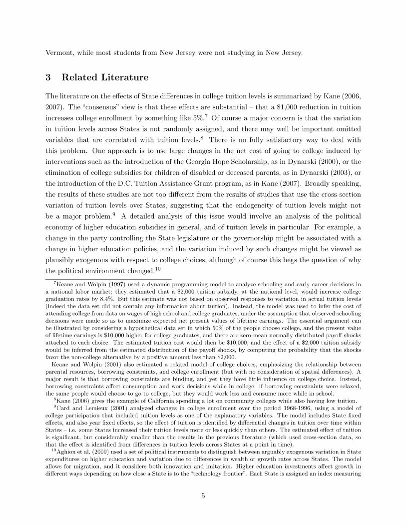
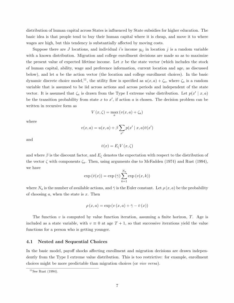
The figure on the left uses data on State & Local Finances from the Census of Governments. Percapita State and local expenditures on higher education for each State in 2012 are plotted against thecorresponding amounts for 1992, with a regression line superimposed. The figure on the right usesdata from IPEDS. The y-variable is calculated by summing instructional expenditures over all publiccolleges in each State, and dividing by the number of high school graduates born in that State whowere in the age range 22− 36 in the 1990 Census. The x−variable is an enrollment-weighted averageof sticker prices in public colleges in each State in 1984. Two regression lines are superimposed (yon x and x on y).

2.1 Tuition and Higher Education Expenditures

States spend substantial amounts on higher education, and there are large and persistent differences in

these expenditures across States. Figure 2.2 shows the variation in (nominal) per capita expenditures

across States in 1992 and 2012, using data from the Census of Governments. The magnitude of these

expenditures suggests that a more highly educated workforce is a major goal of State economic

policies, perhaps because of human capital externalities. Figure 2.2 also shows tuition levels in

public universities in 1984 (when the people in the NLSY cohort were aged 19 to 25), plotted against

a measure of expenditures per student in these universities. Although differences in tuition levels

and expenditures are correlated across States, there is considerable independent variation in these

variables.

A common assumption in the literature on the relationship between college enrollment and cost

is that the relevant measure of tuition is the in-state tuition level, given that most students attend

college in their home State. This is a crude approximation. On average, about 20% of college

freshmen in 2012 enrolled in an out of State college.5 Moreover, this proportion varies greatly across

States. At one extreme, the proportion of both imported and exported students was close to 10%

for California and Texas.6 At the other extreme, most of the freshmen in Vermont were not from

5See nces.ed.gov/programs/digest/d13/tables/dt13 309.20.asp?current=yes6The proportion of imported students is the number of nonresident students as a fraction of total enrollments in

the State, while the proportion of exported students is the number of students from this State attending college out ofstate, as a proportion of all students from this State.

4

Vermont, while most students from New Jersey were not studying in New Jersey.

3 Related Literature

The literature on the effects of State differences in college tuition levels is summarized by Kane (2006,

2007). The “consensus” view is that these effects are substantial – that a $1,000 reduction in tuition

increases college enrollment by something like 5%.7 Of course a major concern is that the variation

in tuition levels across States is not randomly assigned, and there may well be important omitted

variables that are correlated with tuition levels.8 There is no fully satisfactory way to deal with

this problem. One approach is to use large changes in the net cost of going to college induced by

interventions such as the introduction of the Georgia Hope Scholarship, as in Dynarski (2000), or the

elimination of college subsidies for children of disabled or deceased parents, as in Dynarski (2003), or

the introduction of the D.C. Tuition Assistance Grant program, as in Kane (2007). Broadly speaking,

the results of these studies are not too different from the results of studies that use the cross-section

variation of tuition levels over States, suggesting that the endogeneity of tuition levels might not

be a major problem.9 A detailed analysis of this issue would involve an analysis of the political

economy of higher education subsidies in general, and of tuition levels in particular. For example, a

change in the party controlling the State legislature or the governorship might be associated with a

change in higher education policies, and the variation induced by such changes might be viewed as

plausibly exogenous with respect to college choices, although of course this begs the question of why

the political environment changed.10

7Keane and Wolpin (1997) used a dynamic programming model to analyze schooling and early career decisions ina national labor market; they estimated that a $2,000 tuition subsidy, at the national level, would increase collegegraduation rates by 8.4%. But this estimate was not based on observed responses to variation in actual tuition levels(indeed the data set did not contain any information about tuition). Instead, the model was used to infer the cost ofattending college from data on wages of high school and college graduates, under the assumption that observed schoolingdecisions were made so as to maximize expected net present values of lifetime earnings. The essential argument canbe illustrated by considering a hypothetical data set in which 50% of the people choose college, and the present valueof lifetime earnings is $10,000 higher for college graduates, and there are zero-mean normally distributed payoff shocksattached to each choice. The estimated tuition cost would then be $10,000, and the effect of a $2,000 tuition subsidywould be inferred from the estimated distribution of the payoff shocks, by computing the probability that the shocksfavor the non-college alternative by a positive amount less than $2,000.

Keane and Wolpin (2001) also estimated a related model of college choices, emphasizing the relationship betweenparental resources, borrowing constraints, and college enrollment (but with no consideration of spatial differences). Amajor result is that borrowing constraints are binding, and yet they have little influence on college choice. Instead,borrowing constraints affect consumption and work decisions while in college: if borrowing constraints were relaxed,the same people would choose to go to college, but they would work less and consume more while in school.

8Kane (2006) gives the example of California spending a lot on community colleges while also having low tuition.9Card and Lemieux (2001) analyzed changes in college enrollment over the period 1968-1996, using a model of

college participation that included tuition levels as one of the explanatory variables. The model includes State fixedeffects, and also year fixed effects, so the effect of tuition is identified by differential changes in tuition over time withinStates – i.e. some States increased their tuition levels more or less quickly than others. The estimated effect of tuitionis significant, but considerably smaller than the results in the previous literature (which used cross-section data, sothat the effect is identified from differences in tuition levels across States at a point in time).

10Aghion et al. (2009) used a set of political instruments to distinguish between arguably exogenous variation in Stateexpenditures on higher education and variation due to differences in wealth or growth rates across States. The modelallows for migration, and it considers both innovation and imitation. Higher education investments affect growth indifferent ways depending on how close a State is to the “technology frontier”. Each State is assigned an index measuring

5

As was shown in Figure 2.2 above, differences in support for higher education across States are

highly persistent in recent years. Goldin and Katz (1999) show that these differences are in fact

persistent over a much longer period of time, and they explain why:

“To sum up, newer states with a high share of well-to-do families and scant presence

of private universities in 1900 became the leaders in public higher education by 1930.

They remain so today.”

As Bound et al. (2004) point out, some of these differences across States might be related to other

unmeasured differences in factors affecting college choices. For example, heavy industries requiring

a lot of engineers and scientists might be located in places where conditions are favorable in terms of

availability of natural resources, but unfavorable in that they happen to be populated by people who

are skeptical about the value of higher education. In that case, the business community might push

for more investment in public universities, and this would lead to a downward bias in estimates of the

response to policy variables. On the other hand, Goldin and Katz (1999) argue that wealthier families

are more likely to expect that their children will go to college, and indeed when they use automobiles

per capita as a proxy for the level of wealth in the State, they find a positive relationship between

wealth and public expenditures on higher education; this would lead to an upward bias in estimates

of the response to policy variables. But although bias in one direction or the other cannot be ruled

out, it seems reasonable to expect that differences in State policies arising from circumstances that

prevailed many years ago would not be strongly related to unmeasured differences in determinants

of college choices for recent cohorts (such as the NLSY79 cohort analyzed in this paper).

Bound et al. (2004) and Groen (2004) sidestep the issue of what causes changes in the number of

college graduates in a State, and focus instead on the relationship between the flow of new graduates

in a State and the stock of graduates working in that State some time later. They conclude that this

relationship is weak, indicating that the scope for State policies designed to affect the educational

composition of the labor force is limited. The empirical results presented here indicate that it is

important to understand the sources of the variation in the flow of new graduates before drawing

policy conclusions. This is discussed in Section 6 below.

4 A Life-Cycle Model of Expected Income Maximization

The empirical results in Kennan and Walker (2011) indicate that high school graduates migrate

across States in response to differences in expected income. This paper analyzes the college choice

and migration decisions of high-school graduates, using an extension of the dynamic programming

model developed in Kennan and Walker (2011). The aim is to quantify the relationship between

college choice and migration decisions, on the one hand, and geographical differences in college costs

and expected incomes on the other. The model can be used to analyze the extent to which the

distance to the frontier, based on patent data. In States close to the frontier, the estimated effect of spending on researchuniversities is positive, but the estimated effect is negative for States that are far from the frontier. The model explainsthis in terms of a tradeoff between using labor to innovate or to imitate.

6

distribution of human capital across States is influenced by State subsidies for higher education. The

basic idea is that people tend to buy their human capital where it is cheap, and move it to where

wages are high, but this tendency is substantially affected by moving costs.

Suppose there are J locations, and individual i’s income yij in location j is a random variable

with a known distribution. Migration and college enrollment decisions are made so as to maximize

the present value of expected lifetime income. Let x be the state vector (which includes the stock

of human capital, ability, wage and preference information, current location and age, as discussed

below), and let a be the action vector (the location and college enrollment choices). In the basic

dynamic discrete choice model,11, the utility flow is specified as u(x, a) + ζa, where ζa is a random

variable that is assumed to be iid across actions and across periods and independent of the state

vector. It is assumed that ζa is drawn from the Type I extreme value distribution. Let p(x′ | x, a)

be the transition probability from state x to x′, if action a is chosen. The decision problem can be

written in recursive form as

V (x, ζ) = maxa

(v(x, a) + ζa)

where

v(x, a) = u(x, a) + β∑x′

p(x′ | x, a)v(x′)

and

v(x) = EζV (x, ζ)

and where β is the discount factor, and Eζ denotes the expectation with respect to the distribution of

the vector ζ with components ζa. Then, using arguments due to McFadden (1974) and Rust (1994),

we have

exp (v(x)) = exp (γ)

Na∑k=1

exp (v(x, k))

whereNa is the number of available actions, and γ is the Euler constant. Let ρ (x, a) be the probability

of choosing a, when the state is x. Then

ρ (x, a) = exp (v (x, a) + γ − v (x))

The function v is computed by value function iteration, assuming a finite horizon, T . Age is

included as a state variable, with v ≡ 0 at age T + 1, so that successive iterations yield the value

functions for a person who is getting younger.

4.1 Nested and Sequential Choices

In the basic model, payoff shocks affecting enrollment and migration decisions are drawn indepen-

dently from the Type I extreme value distribution. This is too restrictive: for example, enrollment

choices might be more predictable than migration choices (or vice versa).

11See Rust (1994).

7

Suppose the choices are arranged in an array with m rows (for locations), and n columns (for

enrollment choices). The model associates continuation values vij with row i and column j, and

there are payoff shocks ζi associated with each row, and κζ ′j associated with each column, where the

shocks are drawn independently from the Type I extreme value distribution, with κ > 0. Then if

row i has been chosen, the column choice is determined by

j = arg maxk

(vik + ζi + κζ ′k

)The (conditional) probability of choosing column j is

ρ (j | i) =exp

(vijκ

)n∑k=1

exp(vikκ

)and the expected value of the row, vi, is given by

exp (vi) = exp (κγ)

(n∑k=1

exp(vikκ

))κ

If row i is chosen before the column shocks are realized (with the understanding that these shocks

will be realized before the column is chosen) then the row choice is determined by

i = arg maxs

(vs + ζs)

The probability of choosing row i is

ρ0 (i) =exp (vi)m∑s=1

exp (vs)

and the expected value of the whole array is

v0 = γ + log

(m∑s=1

exp (vs)

)

= γ + log

(m∑s=1

exp (κγ)

(n∑k=1

exp(vskκ

))κ)

= (1 + κ) γ + logm+ log

m∑i=1

n∑j=1

exp(vijκ

)κ

8

The choice probabilities are then given by

Prob (dij = 1) = ρ (j | i) ρ0 (i)

=exp

(vijκ

)n∑k=1

exp(vikκ

)(

n∑k=1

exp(vikκ

))κm∑s=1

(n∑k=1

exp(vskκ

))κIf κ = 1 (or if m = 1 or n = 1), this reduces to the standard logit formula for the choice probabilities.

The Nested Logit Model discussed by McFadden (1978) gives these same choice probabilities,

but with a different interpretation: the continuation value associated with each choice is specified

as vij + yij , where yij is a generalized extreme value random vector, with joint distribution function

F (y) given by

F (y) = exp

(−

m∑i=1

Yi

)

Y1κi =

n∑j=1

exp(−yijκ

)

subject to the restriction 0 < κ ≤ 1 (which ensures that the density function is non-negative).12

In this interpretation all of the shocks are realized before any choices are made. In the present

context, the period length is taken to be a year, and the timing of the location and enrollment

choices within the year is necessarily fuzzy, so various interpretations are possible, and each is just

a rough approximation of the way that decisions are actually made. The estimated version of the

model assumes that location choices are made before enrollment choices (but the reverse ordering

gives similar results).

4.2 State Variables and Flow Payoffs

Let ` =(`0, `1

)denote the current and previous location, let ω be a vector recording wage information

at these locations, and let ξ denote current enrollment status (with the convention that ξ = 0 means

that the individual is not enrolled in college, and otherwise ξ represents the college type). The state

vector x consists of `, ω, education level achieved so far, ability, parental education, family income,

home location and age.13

The deterministic part of the flow payoff is specified as

uh (x, j) = α0 (e)+α1

(1− T

(`0))w(g, e, b, `0, ω, ξ

)+α2Y

(`0)

+αHχ(`0 = h

)−Ch

(`0, ξ

)−∆ (x, j)

12See Borsch-Supan (1990). Note that the sequential choice interpretation allows κ > 1.13As in Kennan and Walker (2011), a limited (location) history approximation is used to reduce the size of the state

space in a way that takes advantage of the low migration rates seen in the data.

9

Here the first term refers to consumption values associated with different education levels. The second

term refers to after-tax wage income in the current location; the gross wage depends on age, schooling

and ability, as discussed above, and T(`0)

is the tax rate in the current location. This is augmented

by the amenity variable Y(`0). The parameter αH is a premium that allows each individual to have

a preference for their home location (χ denotes an indicator). The cost of attending a college of type

ξ in location ` for a person whose home location is h is denoted by Ch (`, ξ), with Ch (`, 0) = 0. The

cost of moving from `0 to `j is represented by ∆ (x, j).

4.3 Enrollment Decisions

In simple models of higher education choices, high school graduates choose whether to give up four

or five years worth of earnings at high school wages in order to earn a college wage premium for the

remaining forty years or so. In practice, the choices are more complicated. While many students

enroll in college immediately after finishing high school, and stay in college continuously until they

graduate, many others enroll in college after first spending some time in the labor force, or leave

college without finishing a degree, either permanently or temporarily, on enroll in two-year colleges,

with the possibility of subsequently transferring to a four-year college.14 Accordingly, the model

analyzed here treats college choices as the outcome of a sequence of decisions on whether to enroll

in one of several types of college, with uncertainty about whether enrollment will lead to graduation

with a degree.

The specification of the model involves the usual tradeoff between realism and computation; in

particular, since there are many locations, and location is an essential state variable, it is necessary

to use a coarse specification of the other state variables so that the state space does not become too

big. For this reason, there are just three levels of schooling: high school (12 or 13 years of schooling

completed), some college (14 or 15 years) and college graduate (16 years or more).

In each period, there is a choice of whether to enroll in college. There are four types of college:

community colleges, other public colleges and universities, and private colleges at two quality levels.15

The college types differ with respect to tuition, State subsidies, financial aid, graduation probabilities,

and psychic costs and benefits. Enrollment choices are influenced by ability, parental schooling and

family income, represented by permanent state variables, which are restricted to just two values,

high or low.16

4.4 Wages

The wage of individual i in location j at age g in year t is specified as

wijt = µj (ei) + υij (ei) +G(ei, Xi, gi) + εijt(e) + ηi

14Agan (2014) presents a detailed description of the various paths taken by college students, using NLSY79 data.15Fu (2014) uses a similar set of college types in her analysis of equilibrium in the college admissions market.16Again, binary state variables are used here in order to keep the state space manageable.

10

where e is schooling level, µj is the mean wage in location j (for each level of schooling), υ is a per-

manent location match effect, G(e,X, g) represents the effects of observed individual characteristics,

η is an individual effect that affects wages in the same way in all locations, and ε is a transient effect.

The random variables η, υ and ε are assumed to be independently and identically distributed across

individuals and locations, with mean zero. It is also assumed that the realizations of υ and η are

seen by the individual (although υij (ei) is seen by i only after moving to j with education ei).

The function G is specified as a piecewise-quadratic function of age g, with an interaction between

ability and education:

G(e, b, g) =

θeb+ y∗e − ce (g − g∗e)2 g ≤ g∗e

θeb+ y∗e g ≥ g∗e

where b is measured ability, y∗e is the peak wage for education level e, and g∗e is age at the peak.

Thus both the shape of the age-earnings profile and the ability premium are specified separately for

each level of education, with four parameters to be estimated (θe, y∗e , ce, and g∗e).

17

The relationship between wages and actions is governed by the difference between the quality

of the match in the current location, measured by µj (e) + υij (e) + G(e, b, g), and the prospect of

obtaining a better match in another location or at a higher level of schooling. The other components

of wages have no bearing on migration or enrollment decisions, since they are added to the wage in

the same way no matter what decisions are made.

4.4.1 Stochastic Wage Components

Since the realized value of the location match component υ is a state variable, it is convenient to

specify this component as a random variable with a discrete distribution, and compute continua-

tion values at the support points of this distribution. For given support points, the best discrete

approximation F for any distribution F assigns probabilities so as to equate F with the average

value of F over each interval where F is constant. If the support points are variable, they are chosen

so that F assigns equal probability to each point.18 Thus if the distribution of the location match

component υ were known, the wage prospects associated with a move to State k could be represented

by a distribution with equally weighted support points µk + υ (qr) , 1 ≤ r ≤ R, where υ (qr) is the qr

quantile of the distribution of υ, with

qr =2r − 1

2R

for 1 ≤ r ≤ R. The distribution of υ is in fact not known, but it is assumed to be symmetric around

zero. Thus for example with R = 3, the distribution of µj + υij in each State for each education

level is approximated by a distribution that puts mass 13 on µj (the median of the distribution of

17This is a version of the “flat-spot” specification developed by Heckman et al. (1998). In the present context, themodel uses expected earnings at ages outside the range of the data to explain enrollment and migration choices atyounger ages, and assuming that earnings are constant after the peak limits the possibility that the model mightgenerate spurious explanations of these choices driven by implausible earnings at later ages.

18See Kennan (2006)

11

µj + υij), with mass 13 on µj ± υ0 , where υ0 is a parameter to be estimated.

Measured earnings in the NLSY are highly variable, even after controlling for education and

ability. Moreover, while some people have earnings histories that are well approximated by a concave

age-earnings profile, others have earnings histories that are quite irregular. In other words, the

variability of earnings over time is itself quite variable across individuals. It is important to use

a wage components model that is flexible enough to fit these data, in order to obtain reasonable

inferences about the relationship between measured earnings and the realized values of the location

match component. The wage components at each education level are specified as in Kennan and

Walker (2011). The fixed effect η is assumed to be uniformly and symmetrically distributed around

zero, with three points of support, so that there is one parameter to be estimated. The transient

component ε should be drawn from a continuous distribution that is flexible enough to account for the

observed variability of earnings. It is assumed that ε is drawn from a normal distribution with zero

mean for each person, but with a variance that differs across people. Specifically, person i initially

draws σε (i) from a uniform discrete distribution with two support points (which are parameters to

be estimated), and subsequently draws εit from a normal distribution with mean zero and standard

deviation σε (i), with εit drawn independently in each period.

4.5 College Costs

Aside from consumption values and expected income, all of the variables in the model that affect

college choices do so by changing the costs associated with being in college. Earnings while enrolled

in college are ignored. The college cost depends on ability, b, and on age, g (relative to an initial age

g0 which is set to 19). The cost also depends on resident and nonresident tuition rates, τr (`, ξ) and

τn (`, ξ), expenditure on higher education, y (`, ξ), financial aid (scholarships), s (`, ξ), and parents’

education and family income. Let dm and df be indicators of whether the mother and the father

have some college education, and let yf be an indicator of whether family income is high or low. Let

Ξ be the set of upper-tier colleges. The cost of attending a college of type ξ is specified as

C (`, ξ) = δ0 (ξ) + δ1 (ξ) τ (`, ξ) + δ2 (ξ)E (`, ξ) + δ3b+ δ4bχ (ξ ∈ Ξ) + δ5dm + δ6df + δ7y + δ8 (g − g0)

+ (δ9 (ξ) + δ10b+ δ11dm + δ12df + δ13yf ) s (`, ξ) + (δ14 + δ15b)χ (e = 1) + δ16χ (ξ = ξ−1)χ (e < 2)

where tuition is given by

τ (`, ξ) = χ (` = h) τr (`, ξ) + χ (` 6= h) τn (`, ξ)

(with τr = τn for private colleges). For each college type ξ, δ0 (ξ) measures the disutility of the effort

involved in taking college courses (offset by the utility of life as a student); effort cost depends on

ability (δ3), especially in upper-tier colleges (δ4), and the cost may be higher as students advance

through college, especially for low-ability students (δ14 + δ15b).19 The tuition measures are averages

19In general it is not possible to distinguish between the nonpecuniary costs of college (δ0) and the nonpecuniarybenefits of having a college education (α0). The income coefficient is identified by the migration component of the

12

over each college type within a State; it is assumed that the actual net tuition is a linear function of

the State average tuition measures, and δ1 (ξ) represents the slope of this function, for each college

type. Similarly, δ2 (ξ) measures the extent to which higher education expenditures reduce the cost of

college, without specifying any particular channel through which this effect operates. The effect of

scholarships is also measured separately for each college type, and in addition it depends on ability,

parental education, and family income. The point here is that scholarships are largely allocated on

the basis of merit or need; a college that has a large scholarship budget is more attractive (given

tuition and expenditure levels), but the size of the scholarship budget is obviously more relevant for

students who are more likely to be eligible for scholarships. Finally, persistence in enrollment choices

is captured by the parameter δ16.

4.6 Moving Costs

Moving costs are specified as in Kennan and Walker (2011). Let D(`0, j

)be the distance from the

current location to location j, and let A(`0) be the set of locations adjacent to `0 (where States are

adjacent if they share a border). The moving cost is specified as

∆ (x, j) =(γ0 (e) + γ1D

(`0, j

)− γ2χ

(j ∈ A

(`0))− γ3χ

(j = `1

)+ γ4g − γ5nj

)χ(j 6= `0

)Thus the moving cost varies with education. The observed migration rate is much higher for college

graduates than for high school graduates, and the model can account for this either through differ-

ences in potential income gains or differences in the cost of moving. The moving cost is an affine

function of distance (which is measured as the great circle distance between population centroids).

Moves to an adjacent location may be less costly (because it is possible to change States while re-

maining in the same general area). A move to a previous location may also be less costly, relative to

moving to a new location. In addition, the cost of moving is allowed to depend on age, g. Finally, it

may be cheaper to move to a large location, as measured by population size nj .

4.7 Transition Probabilities

The state vector can be written as x = (x, g), where x =(e, `0, `1, x0υ

)and where x0υ and x1υ index

the realizations of the location match component of wages in the current and previous locations. Let

qb (e, ξ) denote the probability of advancing from education level e to e+ 1, for someone with ability

model. So the proportion who would choose college is known if there is no college cost, and if there is no differencebetween education levels except that college graduates earn more. Suppose the prediction is that the proportion goingto college is 80%, and suppose that only 30% choose college in the data. The model might explain this by saying thatgoing to college is costly. Alternatively, it might be explained by saying that there are nonpecuniary payoffs associatedwith the different education levels. The specification of costs and returns used here imposes an exclusion restrictionthat distinguishes one from the other: the transition probabilities are more favorable for high-ability people, but thenonpecuniary benefits of having a college education are the same for both types. This assumption is arbitrary. Butthe main point of the model is not to make these distinctions, but rather to estimate the responses to changes in thepolicy variables.

13

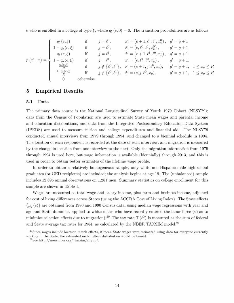
b who is enrolled in a college of type ξ, where qb (e, 0) = 0. The transition probabilities are as follows

p(x′ | x

)=

qb (e, ξ) if j = `0, x′ =(e+ 1, `0, `1, x0υ

), g′ = g + 1

1− qb (e, ξ) if j = `0, x′ =(e, `0, `1, x0υ

), g′ = g + 1

qb (e, ξ) if j = `1, x′ =(e+ 1, `1, `0, x1υ

), g′ = g + 1

1− qb (e, ξ) if j = `1, x′ =(e, `1, `0, x1υ

), g′ = g + 1,

qb(e,ξ)R if j /∈

{`0, `1

}, x′ = (e+ 1, j, `0, xυ), g′ = g + 1, 1 ≤ xυ ≤ R

1−qb(e,ξ)R if j /∈

{`0, `1

}, x′ = (e, j, `0, xυ), g′ = g + 1, 1 ≤ xυ ≤ R

0 otherwise

5 Empirical Results

5.1 Data

The primary data source is the National Longitudinal Survey of Youth 1979 Cohort (NLSY79);

data from the Census of Population are used to estimate State mean wages and parental income

and education distributions, and data from the Integrated Postsecondary Education Data System

(IPEDS) are used to measure tuition and college expenditures and financial aid. The NLSY79

conducted annual interviews from 1979 through 1994, and changed to a biennial schedule in 1994.

The location of each respondent is recorded at the date of each interview, and migration is measured

by the change in location from one interview to the next. Only the migration information from 1979

through 1994 is used here, but wage information is available (biennially) through 2013, and this is

used in order to obtain better estimates of the lifetime wage profile.

In order to obtain a relatively homogeneous sample, only white non-Hispanic male high school

graduates (or GED recipients) are included; the analysis begins at age 19. The (unbalanced) sample

includes 12,895 annual observations on 1,281 men. Summary statistics on college enrollment for this

sample are shown in Table 1.

Wages are measured as total wage and salary income, plus farm and business income, adjusted

for cost of living differences across States (using the ACCRA Cost of Living Index). The State effects

{µj (e)} are obtained from 1980 and 1990 Census data, using median wage regressions with year and

age and State dummies, applied to white males who have recently entered the labor force (so as to

minimize selection effects due to migration).20 The tax rate T(`0)

is measured as the sum of federal

and State average tax rates for 1984, as calculated by the NBER TAXSIM model.21

20Since wages include location match effects, if mean State wages were estimated using data for everyone currentlyworking in the State, the estimated match effect distribution would be biased.

21See http://users.nber.org/˜taxsim/allyup/.

14

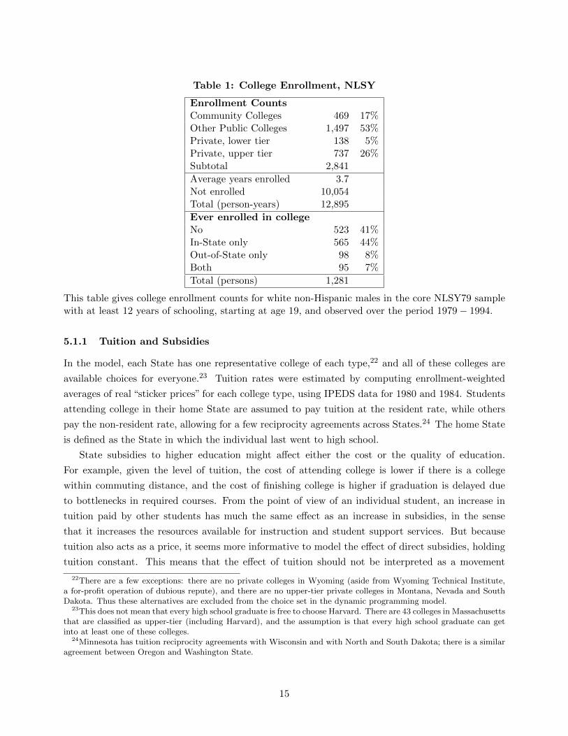
Table 1: College Enrollment, NLSY

Enrollment CountsCommunity Colleges 469 17%Other Public Colleges 1,497 53%Private, lower tier 138 5%Private, upper tier 737 26%Subtotal 2,841

Average years enrolled 3.7Not enrolled 10,054Total (person-years) 12,895

Ever enrolled in collegeNo 523 41%In-State only 565 44%Out-of-State only 98 8%Both 95 7%

Total (persons) 1,281

This table gives college enrollment counts for white non-Hispanic males in the core NLSY79 samplewith at least 12 years of schooling, starting at age 19, and observed over the period 1979− 1994.

5.1.1 Tuition and Subsidies

In the model, each State has one representative college of each type,22 and all of these colleges are

available choices for everyone.23 Tuition rates were estimated by computing enrollment-weighted

averages of real “sticker prices” for each college type, using IPEDS data for 1980 and 1984. Students

attending college in their home State are assumed to pay tuition at the resident rate, while others

pay the non-resident rate, allowing for a few reciprocity agreements across States.24 The home State

is defined as the State in which the individual last went to high school.

State subsidies to higher education might affect either the cost or the quality of education.

For example, given the level of tuition, the cost of attending college is lower if there is a college

within commuting distance, and the cost of finishing college is higher if graduation is delayed due

to bottlenecks in required courses. From the point of view of an individual student, an increase in

tuition paid by other students has much the same effect as an increase in subsidies, in the sense

that it increases the resources available for instruction and student support services. But because

tuition also acts as a price, it seems more informative to model the effect of direct subsidies, holding

tuition constant. This means that the effect of tuition should not be interpreted as a movement

22There are a few exceptions: there are no private colleges in Wyoming (aside from Wyoming Technical Institute,a for-profit operation of dubious repute), and there are no upper-tier private colleges in Montana, Nevada and SouthDakota. Thus these alternatives are excluded from the choice set in the dynamic programming model.

23This does not mean that every high school graduate is free to choose Harvard. There are 43 colleges in Massachusettsthat are classified as upper-tier (including Harvard), and the assumption is that every high school graduate can getinto at least one of these colleges.

24Minnesota has tuition reciprocity agreements with Wisconsin and with North and South Dakota; there is a similaragreement between Oregon and Washington State.

15

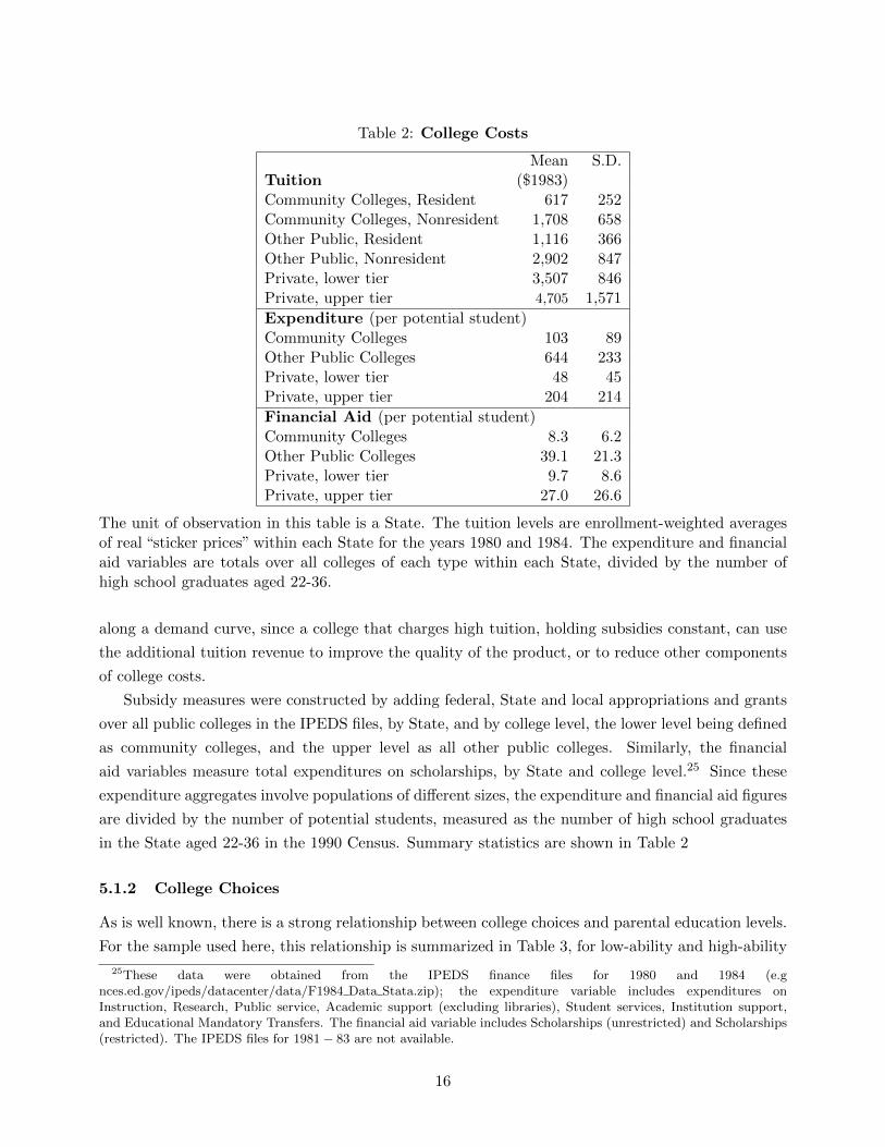
Table 2: College Costs

Mean S.D.Tuition ($1983)Community Colleges, Resident 617 252Community Colleges, Nonresident 1,708 658Other Public, Resident 1,116 366Other Public, Nonresident 2,902 847Private, lower tier 3,507 846Private, upper tier 4,705 1,571

Expenditure (per potential student)Community Colleges 103 89Other Public Colleges 644 233Private, lower tier 48 45Private, upper tier 204 214

Financial Aid (per potential student)Community Colleges 8.3 6.2Other Public Colleges 39.1 21.3Private, lower tier 9.7 8.6Private, upper tier 27.0 26.6

The unit of observation in this table is a State. The tuition levels are enrollment-weighted averagesof real “sticker prices” within each State for the years 1980 and 1984. The expenditure and financialaid variables are totals over all colleges of each type within each State, divided by the number ofhigh school graduates aged 22-36.

along a demand curve, since a college that charges high tuition, holding subsidies constant, can use

the additional tuition revenue to improve the quality of the product, or to reduce other components

of college costs.

Subsidy measures were constructed by adding federal, State and local appropriations and grants

over all public colleges in the IPEDS files, by State, and by college level, the lower level being defined

as community colleges, and the upper level as all other public colleges. Similarly, the financial

aid variables measure total expenditures on scholarships, by State and college level.25 Since these

expenditure aggregates involve populations of different sizes, the expenditure and financial aid figures

are divided by the number of potential students, measured as the number of high school graduates

in the State aged 22-36 in the 1990 Census. Summary statistics are shown in Table 2

5.1.2 College Choices

As is well known, there is a strong relationship between college choices and parental education levels.

For the sample used here, this relationship is summarized in Table 3, for low-ability and high-ability

25These data were obtained from the IPEDS finance files for 1980 and 1984 (e.gnces.ed.gov/ipeds/datacenter/data/F1984 Data Stata.zip); the expenditure variable includes expenditures onInstruction, Research, Public service, Academic support (excluding libraries), Student services, Institution support,and Educational Mandatory Transfers. The financial aid variable includes Scholarships (unrestricted) and Scholarships(restricted). The IPEDS files for 1981 − 83 are not available.

16

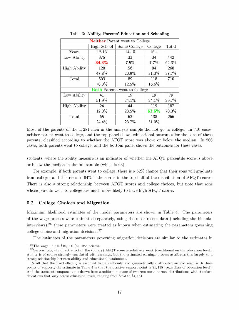
Table 3: Ability, Parents’ Education and Schooling

Neither Parent went to College

High School Some College College Total

Years 12-13 14-15 16+

Low Ability 375 33 34 44284.8% 7.5% 7.7% 62.3%

High Ability 128 56 84 26847.8% 20.9% 31.3% 37.7%

Total 503 89 118 71070.8% 12.5% 16.6%

Both Parents went to College

Low Ability 41 19 19 7951.9% 24.1% 24.1% 29.7%

High Ability 24 44 119 18712.8% 23.5% 63.6% 70.3%

Total 65 63 138 26624.4% 23.7% 51.9%

Most of the parents of the 1, 281 men in the analysis sample did not go to college. In 710 cases,neither parent went to college, and the top panel shows educational outcomes for the sons of theseparents, classified according to whether the AFQT score was above or below the median. In 266cases, both parents went to college, and the bottom panel shows the outcomes for these cases.

students, where the ability measure is an indicator of whether the AFQT percentile score is above

or below the median in the full sample (which is 63).

For example, if both parents went to college, there is a 52% chance that their sons will graduate

from college, and this rises to 64% if the son is in the top half of the distribution of AFQT scores.

There is also a strong relationship between AFQT scores and college choices, but note that sons

whose parents went to college are much more likely to have high AFQT scores.

5.2 College Choices and Migration

Maximum likelihood estimates of the model parameters are shown in Table 4. The parameters

of the wage process were estimated separately, using the most recent data (including the biennial

interviews);26 these parameters were treated as known when estimating the parameters governing

college choice and migration decisions.27

The estimates of the parameters governing migration decisions are similar to the estimates in

26The wage unit is $10, 000 (at 1983 prices).27Surprisingly, the direct effect of the (binary) AFQT score is relatively weak (conditional on the education level).

Ability is of course strongly correlated with earnings, but the estimated earnings process attributes this largely to astrong relationship between ability and educational attainment.

Recall that the fixed effect η is assumed to be uniformly and symmetrically distributed around zero, with threepoints of support; the estimate in Table 4 is that the positive support point is $1, 138 (regardless of education level).And the transient component ε is drawn from a uniform mixture of two zero-mean normal distributions, with standarddeviations that vary across education levels, ranging from $593 to $4, 484.

17

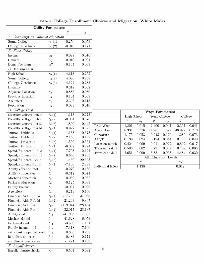
Table 4: College Enrollment Choices and Migration, White Males

Utility Parameters

θ σθ

A. Consumption value of education

Some College α0 (1) -0.256 0.053College Graduate α0 (2) -0.010 0.171

B. Flow Utility

Income α1 0.098 0.010Climate α2 0.010 0.004Home Premium αH 0.164 0.009

C. Moving Cost

High School γ0 (1) 4.613 0.252Some College γ0 (2) 4.090 0.268College Graduate γ0 (3) 4.122 0.283Distance γ1 0.312 0.062Adjacent Location γ2 0.886 0.080Previous Location γ3 0.164 0.009Age effect γ4 2.305 0.113Population γ5 0.083 0.010

D. College Cost

Disutility, college: Pub lo δ0 (1) 1.113 0.273Disutility, college: Pub hi δ0 (2) -0.084 0.376Disutility, college: Pvt lo δ0 (3) 1.800 0.445Disutility, college: Pvt hi δ0 (4) 0.927 0.395Tuition: Public lo δ1 (1) 1.138 0.373Tuition: Public hi δ1 (2) 2.146 0.187Tuition: Private lo δ1 (3) -1.599 0.561Tuition: Private hi δ1 (4) -0.087 0.224Spend/Student: Pub lo δ2 (1) -17.703 2.121Spend/Student: Pub hi δ2 (2) 0.656 0.763Spend/Student: Pvt lo δ2 (3) 11.460 29.693Spend/Student: Pvt hi δ2 (4) -7.160 2.899Ability effect on cost δ3 -0.279 0.160Ability×upper tier δ4 -0.312 0.074Mother’s education δ5 0.069 0.032Father’s education δ6 -0.125 0.033Family Income δ7 -0.067 0.029Age effect δ8 0.279 0.160Financial Aid: Pub lo δ9 (1) -17.762 37.030Financial Aid: Pub hi δ9 (2) 21.243 9.867Financial Aid: Pvt lo δ9 (3) -119.044 128.454Financial Aid: Pvt hi δ9 (4) 32.017 23.137Ability×aid δ10 -41.933 7.302Mother-ed×aid δ11 -41.628 6.953Father-ed×aid δ12 -3.550 7.191Family income×aid δ13 -7.318 7.100extra cost, upper ed level δ14 0.868 0.257hi ability, upper ed δ15 0.483 0.174enrollment persistence δ16 -1.421 0.102

E. Payoff shocks

Enroll/migrate shocks κ 0.504 0.032

Wage Parameters

High School Some College College

θ σθ θ σθ θ σθ

Peak Wage 1.801 0.015 2.400 0.041 2.367 0.041Age at Peak 38.334 0.376 44.961 1.327 48.922 0.713Curvature 1.175 0.053 0.943 0.120 1.285 0.073AFQT 0.139 0.024 0.124 0.044 0.150 0.040Location match 0.424 0.009 0.911 0.022 0.892 0.017Transient s.d. 1 0.593 0.002 0.791 0.007 0.789 0.005Transient s.d. 2 2.651 0.009 3.831 0.053 4.484 0.030

All Education Levelsθ σθ

Individual Effect 1.138 0.012

18

Kennan and Walker (2011). The estimated income coefficient in this model reflects both migration

and college choice decisions; as in the migration model, the effect is highly significant. Ability and

parental education levels have strong effects on college costs (as would be expected, given the data

in Table 3). The sequential structure of the payoff shocks substantially improves the model fit,

and the estimate of κ indicates that migration decisions are much less predictable than enrollment

decisions. The estimated moving costs are decreasing in the level of education, reflecting the positive

relationship between education and migration rates in the data. The age coefficients for both moving

and enrollment costs are quite significant. If these coefficients were zero, the model could still explain

why younger people are more likely to enroll in college, just as they are more likely to move: these

are both investment decisions, and if the net return is positive, it is better to invest sooner rather

than later. The estimates indicate that this human capital explanation is insufficient to fully explain

why observed enrollment and migration rates are decreasing in age.

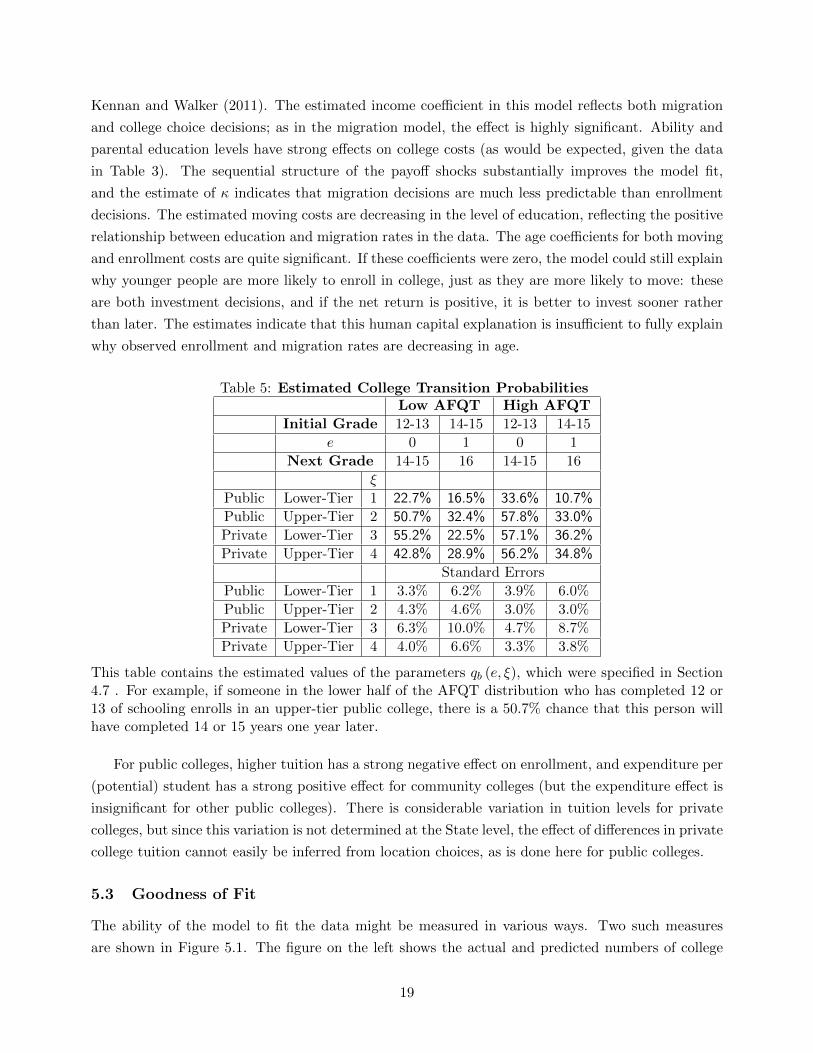
Table 5: Estimated College Transition ProbabilitiesLow AFQT High AFQT

Initial Grade 12-13 14-15 12-13 14-15

e 0 1 0 1

Next Grade 14-15 16 14-15 16

ξ

Public Lower-Tier 1 22.7% 16.5% 33.6% 10.7%

Public Upper-Tier 2 50.7% 32.4% 57.8% 33.0%

Private Lower-Tier 3 55.2% 22.5% 57.1% 36.2%

Private Upper-Tier 4 42.8% 28.9% 56.2% 34.8%

Standard Errors

Public Lower-Tier 1 3.3% 6.2% 3.9% 6.0%

Public Upper-Tier 2 4.3% 4.6% 3.0% 3.0%

Private Lower-Tier 3 6.3% 10.0% 4.7% 8.7%

Private Upper-Tier 4 4.0% 6.6% 3.3% 3.8%

This table contains the estimated values of the parameters qb (e, ξ), which were specified in Section4.7 . For example, if someone in the lower half of the AFQT distribution who has completed 12 or13 of schooling enrolls in an upper-tier public college, there is a 50.7% chance that this person willhave completed 14 or 15 years one year later.

For public colleges, higher tuition has a strong negative effect on enrollment, and expenditure per

(potential) student has a strong positive effect for community colleges (but the expenditure effect is

insignificant for other public colleges). There is considerable variation in tuition levels for private

colleges, but since this variation is not determined at the State level, the effect of differences in private

college tuition cannot easily be inferred from location choices, as is done here for public colleges.

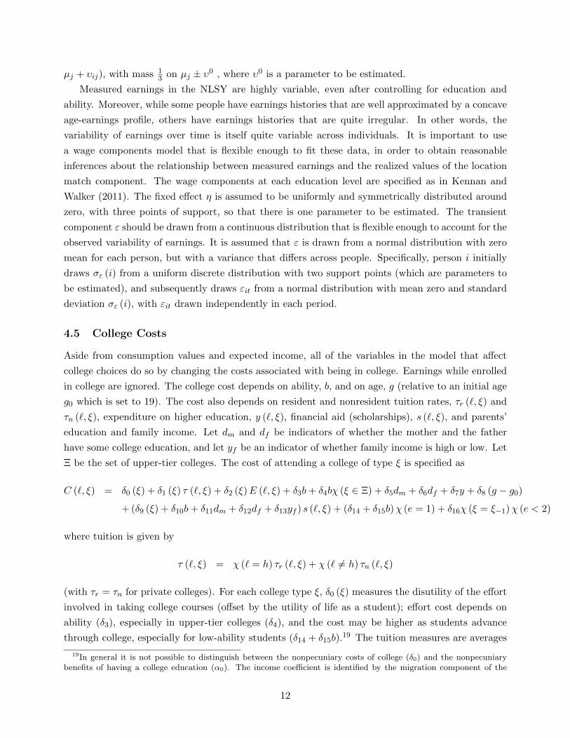
5.3 Goodness of Fit

The ability of the model to fit the data might be measured in various ways. Two such measures

are shown in Figure 5.1. The figure on the left shows the actual and predicted numbers of college

19

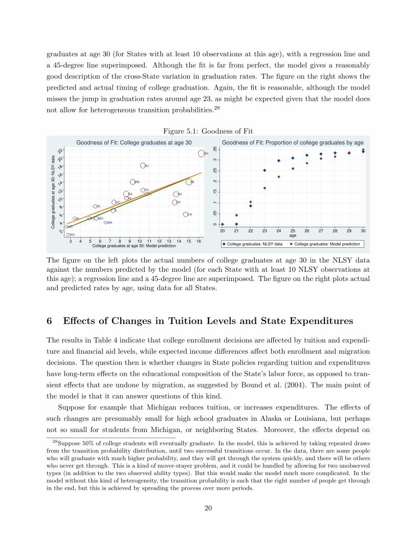
graduates at age 30 (for States with at least 10 observations at this age), with a regression line and

a 45-degree line superimposed. Although the fit is far from perfect, the model gives a reasonably

good description of the cross-State variation in graduation rates. The figure on the right shows the

predicted and actual timing of college graduation. Again, the fit is reasonable, although the model

misses the jump in graduation rates around age 23, as might be expected given that the model does

not allow for heterogeneous transition probabilities.28

Figure 5.1: Goodness of Fit

AL

CA

CT

FL

IL

IN

IA

MA

MIMN

MO

MT

NJ

NYNC

OH

PA

TX

WV

WI

2

4

6

8

10

12

14

16

18

20

22

Colle

ge g

raduate

s a

t age 3

0: N

LS

Y d

ata

3 4 5 6 7 8 9 10 11 12 13 14 15 16College graduates at age 30: Model prediction

Goodness of Fit: College graduates at age 30

0.0

5.1

.15

.2.2

5.3

.35

20 21 22 23 24 25 26 27 28 29 30age

College graduates: NLSY data College graduates: Model prediction

Goodness of Fit: Proportion of college graduates by age

The figure on the left plots the actual numbers of college graduates at age 30 in the NLSY dataagainst the numbers predicted by the model (for each State with at least 10 NLSY observations atthis age); a regression line and a 45-degree line are superimposed. The figure on the right plots actualand predicted rates by age, using data for all States.

6 Effects of Changes in Tuition Levels and State Expenditures

The results in Table 4 indicate that college enrollment decisions are affected by tuition and expendi-

ture and financial aid levels, while expected income differences affect both enrollment and migration

decisions. The question then is whether changes in State policies regarding tuition and expenditures

have long-term effects on the educational composition of the State’s labor force, as opposed to tran-

sient effects that are undone by migration, as suggested by Bound et al. (2004). The main point of

the model is that it can answer questions of this kind.

Suppose for example that Michigan reduces tuition, or increases expenditures. The effects of

such changes are presumably small for high school graduates in Alaska or Louisiana, but perhaps

not so small for students from Michigan, or neighboring States. Moreover, the effects depend on

28Suppose 50% of college students will eventually graduate. In the model, this is achieved by taking repeated drawsfrom the transition probability distribution, until two successful transitions occur. In the data, there are some peoplewho will graduate with much higher probability, and they will get through the system quickly, and there will be otherswho never get through. This is a kind of mover-stayer problem, and it could be handled by allowing for two unobservedtypes (in addition to the two observed ability types). But this would make the model much more complicated. In themodel without this kind of heterogeneity, the transition probability is such that the right number of people get throughin the end, but this is achieved by spreading the process over more periods.

20

individual characteristics. The model has 800 types, classified by home location, and by four binary

characteristics (ability, family income, and mother’s and father’s education). In order to estimate

the effects of changes in college costs (or wages) it is necessary to use the respective value functions

to compute the responses for each type, and then construct a suitably weighted average over types.

The main complication here is that parental education and family income vary considerably across

States. To deal with this, data from the 1970 Census were used to identify households with children

aged 5-13 (corresponding to the ages of the individuals in the NLSY data), and the family income

and parental education data for these children were then tabulated, by State.

The proportion of high-ability types in each State is estimated using the AFQT scores and the

parental education and household income data in the NLSY sample. Surprisingly, the binary family

income variable doesn’t help explain ability differences (there is a slight relationship if parental

education variables are excluded, but there is no effect given parental education). And if just one

parent has been to college, it doesn’t really matter which one. The estimated ability proportions are

applied to the parental education data from the 1970 Census.

6.1 Equilibrium Wage Effects

If policy changes affect the educational composition of the labor force, relative wages might also be

affected. It is true that in the long run, if each individual State is considered as a small open economy,

the factor price equalization theorem implies that wages are invariant to local changes in the supply

of labor at different education levels.29 But there is an extensive literature that considers the supply

and demand for labor without dealing with the general equilibrium effects underlying the factor price

equalization theorem, analyzing the empirical relationship between the return to education and the

relative supplies of workers at different education levels.30 Building on this literature, Fortin (2006)

estimated that the “own-cohort relative supply effect” is about −0.2, meaning that a 10% increase

in the relative supply of college graduates in a State generates a 2% reduction in the college wage

premium, within cohorts spanning 10 years. The policy effect estimates presented below are based

on the assumption that wages do not change, as would be true if the assumptions of the factor

price equalization theorem are empirically valid. But in case wages do actually change, it is clearly

of interest to determine whether such changes are large enough to undo the direct effects of policy

changes, and the results from Fortin (2006) will be used for this purpose.

6.2 Simulation Results: Effects of Changes in Policy Variables

The evolution of the population distribution in the model is computed by iterating the transition

matrix of the Markov chain on the state space. The model specifies choice probabilities ρ (x, a),

where x is the state vector, and a is the choice variable; the next state x′ is then determined by the

transition probabilities q (x, a, x′). There is a frequency distribution p (x) over current states, and

29Similarly, factor price equalization implies that immigration does not affect wages; see Kennan (2013)30See Katz and Murphy (1992) and the many thousands of references thereto

(scholar.google.com/citations?user=MAqEdFMAAAAJ).

21

the model implies a transition matrix T from p (x) to p′ (x) given by

T (p) (x) =∑t∈X

p (t)∑a∈A

ρ (t, a) q (t, a, x)

The effects of changes in the policy variables are computed by first iterating the transition matrix

implied by the values of the policy variables used in the estimation, and then doing the same thing

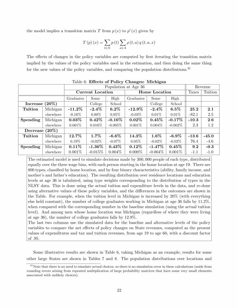
for the new values of the policy variables, and comparing the population distributions.31

Table 6: Effects of Policy Changes: MichiganPopulation at Age 36 Revenue

Current Location Home Location Taxes Tuition

Graduates Some High Graduates Some High

Increase (20%) College School College School

Tuition Michigan -11.2% -2.4% 6.2% -12.9% -2.4% 6.5% 25.2 2.1elsewhere -0.16% 0.00% 0.05% -0.03% 0.01% 0.01% -82.1 2.5

Spending Michigan 0.03% 0.42% -0.16% 0.02% 0.45% -0.17% -10.3 2.6elsewhere 0.001% 0.016% -0.005% 0.001% 0.004% -0.002% 2.3 1.2

Decrease (20%)

Tuition Michigan 12.7% 1.7% -6.6% 14.3% 1.6% -6.9% -13.6 -45.0elsewhere 0.19% -0.02% -0.07% 0.05% -0.02% -0.02% 76.4 -4.6

Spending Michigan 0.11% -1.36% 0.43% 0.12% -1.47% 0.45% 9.2 -0.3elsewhere 0.001% -0.015% 0.004% 0.000% -0.004% 0.001% -1.1 -1.0

The estimated model is used to simulate decisions made by 300, 000 people of each type, distributedequally over the three wage bins, with each person starting in the home location at age 19. There are800 types, classified by home location, and by four binary characteristics (ability, family income, andmother’s and father’s education). The resulting distribution over residence locations and educationlevels at age 36 is tabulated, using type weights corresponding to the distribution of types in theNLSY data. This is done using the actual tuition and expenditure levels in the data, and re-doneusing alternative values of these policy variables, and the differences in the outcomes are shown inthe Table. For example, when the tuition level in Michigan is increased by 20% (with everythingelse held constant), the number of college graduates working in Michigan at age 36 falls by 11.2%,when compared with the corresponding number in the baseline simulation (using the actual tuitionlevel). And among men whose home location was Michigan (regardless of where they were livingat age 36), the number of college graduates falls by 12.9%.The last two columns use the simulated data for the baseline and alternative levels of the policyvariables to compare the net effects of policy changes on State revenues, computed as the presentvalues of expenditures and tax and tuition revenues, from age 19 to age 60, with a discount factorof .95.

Some illustrative results are shown in Table 6, taking Michigan as an example; results for some

other large States are shown in Tables 7 and 8. The population distributions over locations and

31Note that there is no need to simulate actual choices, so there is no simulation error in these calculations (aside fromrounding errors arising from repeated multiplication of large probability matrices that have some very small elementsassociated with unlikely choices).

22

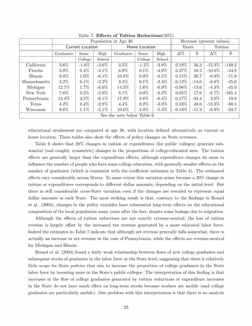
Table 7: Effects of Tuition Reductions(20%)Population at Age 36 Revenue (present values)

Current Location Home Location Taxes Tuition

Graduates Some High Graduates Some High ∆% $ ∆% $

College School College School

California 3.6% -1.0% -3.6% 3.5% -1.2% -3.9% 0.19% 56.3 -12.3% -149.2Florida 5.9% 0.4% -4.1% 6.9% 0.1% -4.9% 0.27% 16.2 -10.0% -44.8Illinois 9.4% 1.0% -6.1% 10.8% 0.9% -6.5% 0.15% 26.7 -6.9% -71.9

Massachusetts 3.2% 0.1% -3.2% 3.4% 0.1% -3.4% -0.12% -14.6 -8.8% -45.6Michigan 12.7% 1.7% -6.6% 14.3% 1.6% -6.9% -0.08% -13.6 -4.3% -45.0New York 7.6% 0.2% -5.8% 8.1% 0.0% -6.2% 0.05% 17.6 -8.7% -165.4

Pennsylvania 13.4% 3.5% -6.1% 17.9% 3.8% -6.4% -0.17% -33.4 2.0% 19.9Texas 4.2% 0.4% -2.8% 4.4% 0.2% -3.0% 0.33% 48.6 -13.3% -80.5

Wisconsin 9.6% 1.1% -5.1% 10.6% 1.0% -5.4% -0.13% -11.3 -6.9% -34.7

See the note below Table 6

educational attainment are compared at age 36, with location defined alternatively as current or

home location. These tables also show the effects of policy changes on State revenues.

Table 6 shows that 20% changes in tuition or expenditures (for public colleges) generate sub-

stantial (and roughly symmetric) changes in the proportions of college-educated men. The tuition

effects are generally larger than the expenditure effects, although expenditure changes do seem to

influence the number of people who have some college education, with generally smaller effects on the

number of graduates (which is consistent with the coefficient estimates in Table 4). The estimated

effects vary considerably across States. To some extent this variation arises because a 20% change in

tuition or expenditures corresponds to different dollar amounts, depending on the initial level. But

there is still considerable cross-State variation even if the changes are rescaled to represent equal

dollar amounts in each State. The most striking result is that, contrary to the findings in Bound

et al. (2004), changes in the policy variables have substantial long-term effects on the educational

composition of the local population many years after the fact, despite some leakage due to migration.

Although the effects of tuition reductions are not exactly revenue-neutral, the loss of tuition

revenue is largely offset by the increased tax revenue generated by a more educated labor force.

Indeed the estimates in Table 7 indicate that although net revenue generally falls somewhat, there is

actually an increase in net revenue in the case of Pennsylvania, while the effects are revenue-neutral

for Michigan and Illinois.

Bound et al. (2004) found a fairly weak relationship between flows of new college graduates and

subsequent stocks of graduates in the labor force at the State level, suggesting that there is relatively

little scope for State policies that aim to increase the proportion of college graduates in the State

labor force by investing more in the State’s public colleges. The interpretation of this finding is that

increases in the flow of college graduates generated by tuition reductions or expenditure increases

in the State do not have much effect on long-term stocks because workers are mobile (and college

graduates are particularly mobile). One problem with this interpretation is that there is no analysis

23

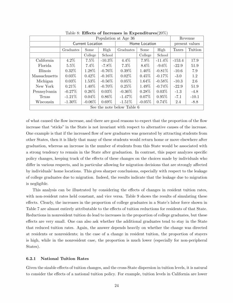
Table 8: Effects of Increases in Expenditures(20%)Population at Age 36 Revenue

Current Location Home Location present values

Graduates Some High Graduates Some High Taxes Tuition

College School College School

California 4.2% 7.5% -10.3% 4.4% 7.9% -11.4% -153.4 17.9Florida 5.5% 7.4% -7.8% 7.3% 8.6% -9.6% -22.9 51.9Illinois 0.32% 1.28% -0.76% 0.39% 1.40% -0.81% -10.6 7.9

Massachusetts 0.03% 0.42% -0.16% 0.02% 0.45% -0.17% -3.0 1.2Michigan 0.03% 1.53% -0.56% 0.05% 1.64% -0.58% -10.3 2.6New York 0.21% 1.40% -0.70% 0.25% 1.49% -0.74% -22.9 51.9

Pennsylvania -0.27% 0.26% 0.03% -0.36% 0.28% 0.03% -1.3 -4.8Texas -1.21% 0.04% 0.86% -1.47% 0.07% 0.95% -7.1 -10.1

Wisconsin -1.30% -0.06% 0.69% -1.51% -0.05% 0.74% 2.4 -8.8

See the note below Table 6

of what caused the flow increase, and there are good reasons to expect that the proportion of the flow

increase that “sticks” in the State is not invariant with respect to alternative causes of the increase.

One example is that if the increased flow of new graduates was generated by attracting students from

other States, then it is likely that many of these students would return home or move elsewhere after

graduation, whereas an increase in the number of students from this State would be associated with

a strong tendency to remain in the State after graduation. In contrast, this paper analyzes specific

policy changes, keeping track of the effects of these changes on the choices made by individuals who

differ in various respects, and in particular allowing for migration decisions that are strongly affected

by individuals’ home locations. This gives sharper conclusions, especially with respect to the leakage

of college graduates due to migration. Indeed, the results indicate that the leakage due to migration

is negligible.

This analysis can be illustrated by considering the effects of changes in resident tuition rates,

with non-resident rates held constant, and vice versa. Table 9 shows the results of simulating these

effects. Clearly, the increases in the proportion of college graduates in a State’s labor force shown in

Table 7 are almost entirely attributable to the effects of tuition reductions for residents of that State.

Reductions in nonresident tuition do lead to increases in the proportion of college graduates, but these

effects are very small. One can also ask whether the additional graduates tend to stay in the State

that reduced tuition rates. Again, the answer depends heavily on whether the change was directed

at residents or nonresidents; in the case of a change in resident tuition, the proportion of stayers

is high, while in the nonresident case, the proportion is much lower (especially for non-peripheral

States).

6.2.1 National Tuition Rates

Given the sizable effects of tuition changes, and the cross-State dispersion in tuition levels, it is natural

to consider the effects of a national tuition policy. For example, tuition levels in California are lower

24

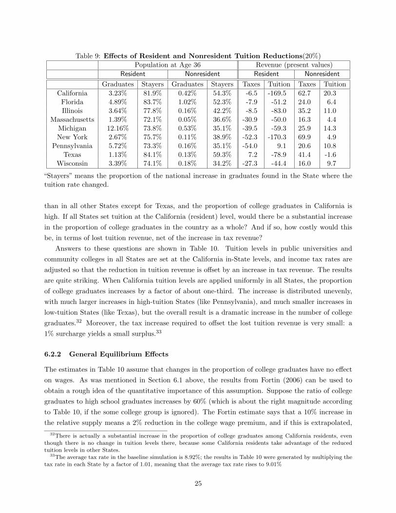
Table 9: Effects of Resident and Nonresident Tuition Reductions(20%)Population at Age 36 Revenue (present values)

Resident Nonresident Resident Nonresident

Graduates Stayers Graduates Stayers Taxes Tuition Taxes Tuition

California 3.23% 81.9% 0.42% 54.3% -6.5 -169.5 62.7 20.3Florida 4.89% 83.7% 1.02% 52.3% -7.9 -51.2 24.0 6.4Illinois 3.64% 77.8% 0.16% 42.2% -8.5 -83.0 35.2 11.0

Massachusetts 1.39% 72.1% 0.05% 36.6% -30.9 -50.0 16.3 4.4Michigan 12.16% 73.8% 0.53% 35.1% -39.5 -59.3 25.9 14.3New York 2.67% 75.7% 0.11% 38.9% -52.3 -170.3 69.9 4.9

Pennsylvania 5.72% 73.3% 0.16% 35.1% -54.0 9.1 20.6 10.8Texas 1.13% 84.1% 0.13% 59.3% 7.2 -78.9 41.4 -1.6

Wisconsin 3.39% 74.1% 0.18% 34.2% -27.3 -44.4 16.0 9.7

“Stayers” means the proportion of the national increase in graduates found in the State where thetuition rate changed.

than in all other States except for Texas, and the proportion of college graduates in California is

high. If all States set tuition at the California (resident) level, would there be a substantial increase

in the proportion of college graduates in the country as a whole? And if so, how costly would this

be, in terms of lost tuition revenue, net of the increase in tax revenue?

Answers to these questions are shown in Table 10. Tuition levels in public universities and

community colleges in all States are set at the California in-State levels, and income tax rates are

adjusted so that the reduction in tuition revenue is offset by an increase in tax revenue. The results

are quite striking. When California tuition levels are applied uniformly in all States, the proportion

of college graduates increases by a factor of about one-third. The increase is distributed unevenly,

with much larger increases in high-tuition States (like Pennsylvania), and much smaller increases in

low-tuition States (like Texas), but the overall result is a dramatic increase in the number of college

graduates.32 Moreover, the tax increase required to offset the lost tuition revenue is very small: a

1% surcharge yields a small surplus.33

6.2.2 General Equilibrium Effects

The estimates in Table 10 assume that changes in the proportion of college graduates have no effect

on wages. As was mentioned in Section 6.1 above, the results from Fortin (2006) can be used to

obtain a rough idea of the quantitative importance of this assumption. Suppose the ratio of college

graduates to high school graduates increases by 60% (which is about the right magnitude according

to Table 10, if the some college group is ignored). The Fortin estimate says that a 10% increase in

the relative supply means a 2% reduction in the college wage premium, and if this is extrapolated,

32There is actually a substantial increase in the proportion of college graduates among California residents, eventhough there is no change in tuition levels there, because some California residents take advantage of the reducedtuition levels in other States.

33The average tax rate in the baseline simulation is 8.92%; the results in Table 10 were generated by multiplying thetax rate in each State by a factor of 1.01, meaning that the average tax rate rises to 9.01%

25

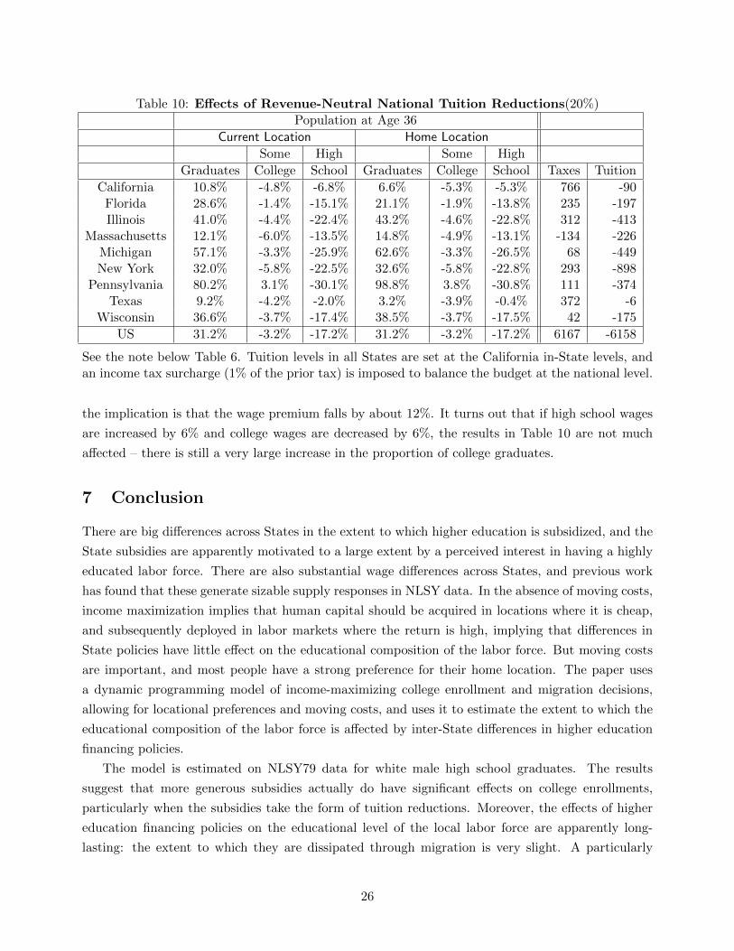
Table 10: Effects of Revenue-Neutral National Tuition Reductions(20%)Population at Age 36

Current Location Home Location

Some High Some High

Graduates College School Graduates College School Taxes Tuition

California 10.8% -4.8% -6.8% 6.6% -5.3% -5.3% 766 -90Florida 28.6% -1.4% -15.1% 21.1% -1.9% -13.8% 235 -197Illinois 41.0% -4.4% -22.4% 43.2% -4.6% -22.8% 312 -413

Massachusetts 12.1% -6.0% -13.5% 14.8% -4.9% -13.1% -134 -226Michigan 57.1% -3.3% -25.9% 62.6% -3.3% -26.5% 68 -449New York 32.0% -5.8% -22.5% 32.6% -5.8% -22.8% 293 -898

Pennsylvania 80.2% 3.1% -30.1% 98.8% 3.8% -30.8% 111 -374Texas 9.2% -4.2% -2.0% 3.2% -3.9% -0.4% 372 -6

Wisconsin 36.6% -3.7% -17.4% 38.5% -3.7% -17.5% 42 -175

US 31.2% -3.2% -17.2% 31.2% -3.2% -17.2% 6167 -6158

See the note below Table 6. Tuition levels in all States are set at the California in-State levels, andan income tax surcharge (1% of the prior tax) is imposed to balance the budget at the national level.

the implication is that the wage premium falls by about 12%. It turns out that if high school wages

are increased by 6% and college wages are decreased by 6%, the results in Table 10 are not much

affected – there is still a very large increase in the proportion of college graduates.

7 Conclusion

There are big differences across States in the extent to which higher education is subsidized, and the

State subsidies are apparently motivated to a large extent by a perceived interest in having a highly

educated labor force. There are also substantial wage differences across States, and previous work

has found that these generate sizable supply responses in NLSY data. In the absence of moving costs,

income maximization implies that human capital should be acquired in locations where it is cheap,

and subsequently deployed in labor markets where the return is high, implying that differences in

State policies have little effect on the educational composition of the labor force. But moving costs

are important, and most people have a strong preference for their home location. The paper uses

a dynamic programming model of income-maximizing college enrollment and migration decisions,

allowing for locational preferences and moving costs, and uses it to estimate the extent to which the

educational composition of the labor force is affected by inter-State differences in higher education

financing policies.

The model is estimated on NLSY79 data for white male high school graduates. The results

suggest that more generous subsidies actually do have significant effects on college enrollments,

particularly when the subsidies take the form of tuition reductions. Moreover, the effects of higher

education financing policies on the educational level of the local labor force are apparently long-

lasting: the extent to which they are dissipated through migration is very slight. A particularly

26

striking implication of the estimated model is that a national tuition policy, set at a uniformly low

level (corresponding to the actual level for California residents), would yield a very large increase in

the proportion of college graduates, and the resulting increase in income tax revenue would almost

completely offset the loss in tuition revenue.

27

Appendix (not for publication)

Estimation Details

The model was estimated by maximum likelihood, using a slightly modified Newton algorithm. Value

functions were computed by backward induction, and numerical derivatives were used to estimate the

gradient of the loglikelihood. The outer product of the gradient was used to estimate the Hessian of

the loglikelihood, and standard errors of the parameter estimates were obtained from the Hessian in

the usual way. Using an MPI-Fortran program, on a cluster with 320 CPUs, the likelihood maximum

was typically reached in less than 24 hours once reasonable starting values for the parameters had

been found.

The wage process was estimated in the same way, using an ordinary Fortran program on a single

computer; this required only a few hours.

28

References

Agan, Amanda Y., “Disaggregating the Returns to College,”January 2014. Unpublished, Princeton

University.

Aghion, P., L. Boustan, C. Hoxby, and J. Vandenbussche, “The Causal Impact of Education

on Economic Growth: Evidence from the United States,” 2009. Unpublished, Harvard University.

Bishop, Kelly C., “A Dynamic Model of Location Choice and Hedonic Valuation,” November 2012.

Unpublished, Washington University in St. Louis.

Borsch-Supan, Axel, “On the compatibility of nested logit models with utility maximization,”

Journal of Econometrics, 1990, 43 (3), 373–388.

Bound, John, Jeffrey Groen, G.Gabor Kezdi, and Sarah Turner, “Trade in university

training: cross-state variation in the production and stock of college-educated labor,” Journal of

Econometrics, 2004, 121 (1-2), 143 – 173. Higher education (Annals issue).

Card, David and Alan B. Krueger, “Does School Quality Matter? Returns to Education and

the Characteristics of Public Schools in the United States,” The Journal of Political Economy,

1992, 100 (1), 1–40.

and Thomas Lemieux, “Dropout and Enrollment Trends in the Postwar Period: What Went

Wrong in the 1970s?,” in Jonathan Gruber, ed., An Economic Analysis of Risky Behavior Among

Youth, Chicago: University of Chicago Press, January 2001, pp. 439–482.

Dynarski, Susan, “Hope for Whom? Financial Aid for the Middle Class and Its Impact on College

Attendance,” National Tax Journal, 2000, 53 (3 Part 2), 629–662.

Dynarski, Susan M., “Does Aid Matter? Measuring the Effect of Student Aid on College Atten-

dance and Completion,” The American Economic Review, 2003, 93 (1), 279–288.

Fortin, Nicole M., “Higher-Education Policies and the College Wage Premium: Cross-State Evi-

dence from the 1990s,” American Economic Review, September 2006, 96 (4), 959–987.

Fu, Chao, “Equilibrium Tuition, Applications, and Admissions and Enrollment in the College Mar-

ket,” Journal of Political Economy, 2014, 122 (2), 225–281.

Gemici, A., “Family migration and labor market outcomes,” January 2011. Unpublished, New York

University.

Goldin, Claudia and Lawrence F. Katz, “The Shaping of Higher Education: The Formative

Years in the United States, 1890 to 1940,” Journal of Economic Perspectives, 1999, 13 (1), 37–62.

Groen, Jeffrey A., “The effect of college location on migration of college-educated labor,” Journal

of Econometrics, 2004, 121 (1-2), 125 – 142. Higher education (Annals issue).

29

Heckman, James J, Lance Lochner, and Christopher Taber, “Explaining Rising Wage In-

equality: Explorations with a Dynamic General Equilibrium Model of Labor Earnings with Het-

erogeneous Agents,” Review of Economic Dynamics, 1998, 1 (1), 1 – 58.

Kane, Thomas J., “Public Intervention in Post-Secondary Education,” in E. Hanushek and

F. Welch, eds., Handbook of the Economics of Education, Vol. 2, Amsterdam, New York and

Oxford: Elsevier Science, North-Holland, 2006, pp. 1369 – 1401.

, “Evaluating the Impact of the D.C. Tuition Assistance Grant Program,” Journal of Human

Resources, 2007, XLII (3), 555–582.

Katz, Lawrence F and Kevin M Murphy, “Changes in Relative Wages, 1963-1987: Supply and

Demand factors,” Quarterly Journal of Economics, 1992, 107 (February), 35–78.

Keane, Michael P. and Kenneth I. Wolpin, “The Career Decisions of Young Men,” Journal of

Political Economy, June 1997, 105 (3), 473–522.

and , “The Effect of Parental Transfers and Borrowing Constraints on Educational Attainment,”

International Economic Review, 2001, 42 (4), 1051–1103.

Kennan, John, “A Note on Discrete Approximations of Continuous Distributions,” 2006. Unpub-

lished, University of Wisconsin–Madison.

, “Open Borders,” Review of Economic Dynamics, April 2013, 16, L1–L13.

and James R. Walker, “The effect of expected income on individual migration decisions,”

Econometrica, January 2011, 79 (1), 211–251.

McFadden, Daniel D,“Conditional logit analysis of qualitative choice behavior,” in Paul Zarembka,

ed., Frontiers in Econometrics, Academic Press, 1974.

McFadden, Daniel L., “Modelling the Choice of Residential Location,” in F. Snickars A. Karlqvist,

L. Lundqvist and J. Weibull, eds., Spatial Interaction Theory and Planning Models, North Holland:

Amsterdam, 1978, chapter 3, pp. 75–96.

Rust, John P., “Structural Estimation of Markov Decision Processes,” in R.F. Engle and D.L.

McFadden, eds., Handbook of Econometrics, Vol. 4, Amsterdam, New York and Oxford: Elsevier

Science, North-Holland, 1994, pp. 3081–3143.

30