Spatial scaling in a changing climate: A hierarchical ...water.columbia.edu/files/2011/11/LimaLall2010Scaling.pdf · assistance of Ercan Kahya, Associate Editor Keywords: Hierarchical

Journal of Hydrology xxx (2010) xxx–xxx

ARTICLE IN PRESS

Contents lists available at ScienceDirect

Journal of Hydrology

journal homepage: www.elsevier .com/ locate / jhydrol

Spatial scaling in a changing climate: A hierarchical bayesian modelfor non-stationary multi-site annual maximum and monthly streamflow

Carlos H.R. Lima *,1, Upmanu LallColumbia University, Water Center, 500 W, 120th Street, Office 842, New York, NY 10027, USA

a r t i c l e i n f o s u m m a r y

Article history:Received 5 April 2009Received in revised form 2 November 2009Accepted 29 December 2009Available online xxxx

This manuscript was handled by A.Bardossy, Editor-in-Chief, with theassistance of Ercan Kahya, Associate Editor

Keywords:Hierarchical Bayesian modelsDrainage area scalingRegionalizationStreamflow spatial scalingFlood frequency analysisFlood flow regionalization

0022-1694/$ - see front matter � 2009 Elsevier B.V. Adoi:10.1016/j.jhydrol.2009.12.045

* Corresponding author. Tel.: +1 212 854 7219.E-mail addresses: [email protected] (C.H.R. L

Lall).1 Supported by Fulbright and CAPES(Brazil) through

Pepsico Foundation.

Please cite this article in press as: Lima, C.H.R.,annual maximum and monthly streamflow. J. H

Several studies have shown that statistics of streamflow time series, in particular empirical moments,scale with physical properties of the drainage basin, such as the catchment area. Those scaling laws havebeen extensively used to estimate statistics of streamflow series at ungauged sites. The role of climate var-iability and change has not been considered in such models. Further, most studies are based on classicalstatistics, where parameter uncertainties are usually neglected or not formally considered. In this paperwe develop and apply hierarchical Bayesian models, to both assess regional and at-site trends in timein a spatial scaling framework, and simultaneously provide a rigorous framework for assessing and reduc-ing parameter and model uncertainties. The models are tested with reconstructed natural inflow seriesfrom over 40 hydropower sites in Brazil with catchments areas varying from 2588 to 823,555 km2. Bothannual maximum flood series and monthly streamflow are considered. Cross-validated results show thatthe Hierarchical Bayesian models are able to skillfully estimate monthly and flood flow probabilitydistribution parameters for sites that were not used in model fitting. The models developed can be usedto provide record augmentation at sites that have short records, or to estimate flow at ungauged sites, evenin the absence of an assumption of time stationarity. Since model uncertainties are accounted for, theprecision of the estimates can be quantified and hypotheses tests for regional and at-site trends can beformally made. A formal inclusion of climate predictors to facilitate seasonal forecasting or climate changescenario development is also feasible. This is indicated, but not developed here.

� 2009 Elsevier B.V. All rights reserved.

Introduction

Regionalization or regional analysis of hydro-climatologicalvariables, such as streamflow, rainfall, evaporation and their asso-ciated statistics (e.g. means, standard deviation, flood quantiles,etc.), has been an active area of research over the last 40 years.The understanding of the spatial variability of these statistics isimportant for hydro-climatological time series and in the water re-sources management. For instance, flood management and designof flood control structures (e.g. dams, bridges, spillways, culverts)usually require the estimate of low exceedance probabilities, e.g.1% for the 100-year flood quantile, which in turn demands a suffi-cient amount of data (no less than 100 years of streamflow recordfor this case) for reliable estimates. Since the desired amount ofdata is rarely available, one wants to use hydroclimatic informa-tion of similar and nearby sites to produce a better, more reliableestimate of the quantiles associated with those low probabilities

ll rights reserved.

ima), [email protected] (U.

Grant # 1650-041, and by the

Lall, U. Spatial scaling in a chanydrol. (2010), doi:10.1016/j.jhy

of occurrence (Stedinger et al., 1993). The recognition that climateis inherently variable and changing also brings the question of howsuch changes should be modeled as part of a formal non-stationaryanalysis (Milly et al., 2008; Jain and Lall, 2001). The work presentedhere addresses aspects of spatial scaling, nonstationarity anduncertainty analysis from a regional perspective working withmultiple time series of monthly flows and annual maximum flow.

At sites with no record of streamflow data (ungauged sites),regional analysis is used to estimate the variable of interest (e.g.the 100-year flood quantile) at sites with historical data of stream-flow available and then relate the estimate with physiographic andgeomorphologic features of the associated region and catchmentbasin. Common features used include drainage area, channel slopeand length, vegetation cover, soil properties, altitude, as well ashistorical and paleo information (e.g. Thomas and Benson, 1970;Stedinger and Cohn, 1986; Martins and Stedinger, 2001). A statis-tical model correlating explanatory and response variables is thenobtained in order to estimate the desired statistics at the ungaugedsite (the problem of prediction in ungauged basins – PUB, seeGupta et al., 2007), where the only information available is relatedto the explanatory variables. Regionalization can also be used toimprove parameter estimates (e.g. the index flood method) and

ging climate: A hierarchical bayesian model for non-stationary multi-sitedrol.2009.12.045

http://dx.doi.org/10.1016/j.jhydrol.2009.12.045

mailto:[email protected]

mailto:[email protected]

http://www.sciencedirect.com/science/journal/00221694

http://www.elsevier.com/locate/jhydrol


watercenter

Stamp

−65 −60 −55 −50 −45 −40 −35 −30−3

5−3

0−2

5−2

0−1

5−1

0−5

0

Daily & Monthly DataDaily Data OnlyMonthly Data Only

Fig. 1. Geographical location of hydropower reservoirs across Brazil. The red linesshow the division of the hydrological basins. Longitude and latitude are shownalong the x and y axes, respectively. (For interpretation of the references to colour inthis figure legend, the reader is referred to the web version of this article.)

2 C.H.R. Lima, U. Lall / Journal of Hydrology xxx (2010) xxx–xxx

ARTICLE IN PRESS

time series augmentation, where only short records of the desiredvariable are present (Salas et al., 1980; Stedinger et al., 1993).

Several attempts have been made to identify spatial scalingattributes of streamflow statistics and catchment physical proper-ties (e.g. Thomas and Benson, 1970; Riggs, 1973; Pandey et al.,1998; Vogel and Sankarasubramanian, 2000; Yue and Gan, 2004;Koscielny-Bunde et al., 2006) or simply to improve the methodsused to link response variables and predictors in current statisticalmodels (e.g. Stedinger and Tasker, 1985; Tasker and Stedinger,1989; Kroll and Stedinger, 1998; Pandey and Nguyen, 1999). Inparticular, annual mean flow and annual peak floods for given re-turn periods have been known for a long time to scale as powerlaws with catchment area (e.g. Benson, 1962; Thomas and Benson,1970; Alexander, 1972), which is the most common variable usedin regionalization due to its availability (one can easily obtain thedrainage area for almost any streamflow site) and reliability (theestimates are very precise). The original scaling relationships havebeen also linked to the literature on multi-fractals where the scal-ing exponents vary by the moment order (Gupta and Waymire,1990; Smith, 1992; Gupta et al., 1994; Becker and Braun, 1999; Vo-gel and Sankarasubramanian, 2000; Sivapalan et al., 2002; Yue andGan, 2004). Poveda et al. (2007) used the long-term water balanceequation to estimate the mean annual flow and then made use ofthe power law to estimate the mean and standard deviation of an-nual floods which in turn were used to calculate annual floods forany given return period. A more comprehensive review of the socalled scaling theory within a nonlinear geophysical frameworkis presented in Gupta et al. (2007), which also discuss the use ofpower laws under global climate changes. However, in none ofthe key papers in this area has a method for assessing temporalvariations in parameters that may be related to climate or otherfactors been discussed. We address this issue.

Following the principle of introduction of more ’structure’ intomodels proposed by the National Research Council (National Re-search Council, 1988), we develop here a hierarchical Bayesianmodel (Gelman et al., 2004), where parameter uncertainties arefully accounted into model outputs and information of differentsources is used in order to shrink those uncertainties and improvethe model reliability. With few exceptions (e.g. Júnior et al., 2005;Poveda et al., 2007; Kwon et al., 2008), regionalization has beenbased on classical statistics, where parameters are assumed sta-tionary in time and space and their associated uncertainties areusually neglected or rely on asymptotic normality assumptionsand are not fully accounted in model outputs. With the frameworkproposed here, we are able to include more information and betterestimate time varying parameters of frequency distributions of an-nual maximum as well as flood quantiles and monthly streamflowsat gauged and ungauged sites, making a significant contribution tothe PUB problem. This paper is organized as follows: in the nextSection we describe the monthly and annual streamflow data. InSection ‘‘Spatial scaling and a bayesian model for the parametersof the probability distribution of annual maximum flood series”we describe a Bayesian model for the parameters of a probabilitydistribution fit to annual maximum flood series. A hierarchicalBayesian model for time varying parameters of the annual maxi-mum series is presented in Section ‘‘Hierarchical bayesian model-ing considering nonstationarity in the scaling of annual maximumflood series”. Finally in Section ‘‘Hierarchical bayesian modeling ofnon-stationary monthly streamflow series” we consider a hierar-chical Bayesian model for monthly streamflow series.

River discharge data

Daily streamflow data of 44 hydropower sites in Brazil (locationshown in Fig. 1) are provided by the System National Operator

Please cite this article in press as: Lima, C.H.R., Lall, U. Spatial scaling in a chanannual maximum and monthly streamflow. J. Hydrol. (2010), doi:10.1016/j.jhy

(ONS), which is the Brazilian institution responsible for definingoperation rules and strategies to maximize the electrical energyproduction across thermal and hydro plants. As displayed inFig. 1, 32 sites are located in nested basins, which together formone of the largest basins (in terms of water flow) in South America,the Paraná basin. The streamflow time series cover the January1931–December 2001 period and span a large range of powercapacities (from 80 MW to 14000 MW) and catchment areas (from322 to 823,555 km2). Most studies of scaling in annual flood fre-quencies have been limited to catchment areas of the order of5000 km2 (e.g. Gupta et al., 1994). To our knowledge, Povedaet al. (2007) was the first article to investigate annual flood scalingstatistics for catchment areas of the order of 1 million km2. Mostsuch analyses consider a nested basin structure, under the assump-tion of a homogeneous climate /rainfall distribution over the re-gion, and topographic/geomorphic controls as the importantdrivers of the scaling relationship of interest between flow anddrainage area. The framework we present here, and the data setused are not limited to this structure. We can allow both spatialand temporal variation in parameters. The latter is formally ex-plored, while the former can be diagnosed through an analysis ofthe site by site variation in model parameters.

The daily series of streamflow used here are reconstructed nat-ural time series, i.e., estimated river flow after accounting for esti-mated water use (e.g. reservoir operation, water withdraws)upstream of the gauge. The annual maximum series are calculatedby taking the maximum daily flow observed for each year of the re-cord. Not all sites have a full record of available data. Fig. 2 showsthe percentage of hydropower reservoirs with available daily flowdata as a function of year. Note that only beyond 1973 one has acomplete set of sites with daily streamflow data. Extension of theserecords to fill in missing values with estimates of the associateduncertainty is one of the motivations of the proposed models.

Monthly inflow series of 45 hydropower sites in Brazil are alsoprovided by ONS. These series cover the 1931–2006 period and arealso reconstructed time series. They have been verified and revisedby the Brazilian National Water Agency (ANA) and do not have any



1930 1940 1950 1960 1970 1980 1990 200055

60

65

70

75

80

85

90

95

100

Perc

enta

ge o

f hyd

ropo

wer

site

s

Year

Fig. 2. Percentage of hydropower reservoirs (out-of 44) with available data of dailystreamflow as a function of year.

C.H.R. Lima, U. Lall / Journal of Hydrology xxx (2010) xxx–xxx 3

ARTICLE IN PRESS

missing values. The geographical location of these sites is displayedin Fig. 1. The associated drainage area varies from 2588 to823,555 km2.

Most of the catchments displayed in Fig. 1 have similar patternsof rainfall seasonality and climate. The rainy season is drivenmainly by the South Atlantic Convergence zone with remote forc-ings from the Tropical Pacific and South Atlantic sea surface tem-peratures (SST). A detailed description of the climate andteleconnection patterns associated with the rainfall regime acrossBrazil can be found in Ropelewski and Halpert (1987), Nogues-Pae-gle and Mo (1997), Grimm (2004), Vera et al. (2006) and referencestherein. Geomorphological attributes of the correspondent drain-age catchments are very diverse, and we do not attempt to inves-

−3 −2 −1 0 1 2

67

89

10

a) Scaling of: Annual Maximum Mean

x

log

( q)

r2 = 0.90

−3 −2 −1 0 1 2

67

89

10

c) Location Parameter

x

log

(a)

r2 = 0.91

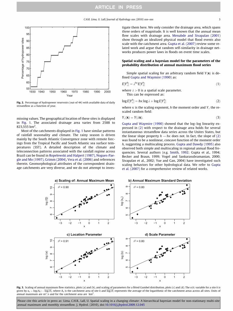
Fig. 3. Scaling of annual maximum flow statistics, plots (a) and (b), and scaling of paramegiven by xk ¼ logðAkÞ � logðAÞ, where Ak is the catchment area of site k and logðAÞ represannual maximum are m3=s and for the catchment area are km2.


tigate them here. We only consider the drainage area, which spansthree orders of magnitude. It is well known that the annual meanflow scales with drainage area. Menabde and Sivapalan (2001)show through an idealized physical model that flood events alsoscale with the catchment area. Gupta et al. (2007) review some re-lated work and argue that random self-similarity in drainage net-works produces power laws in floods on event time scales.

Spatial scaling and a bayesian model for the parameters of theprobability distribution of annual maximum flood series

Simple spatial scaling for an arbitrary random field YðxÞ is de-fined Gupta and Waymire (1990) as:

E½Yhk � ¼ khjE½Yh

1� ð1Þ

where k > 0 is a spatial scale parameter.This can be expressed as:

log E½Yhk � ¼ hj log kþ log E½Yh

1� ð2Þ

where j is the scaling exponent, h the moment order and Yk the re-scaled random field:

YkðxÞ ¼ YðkxÞ: ð3Þ

Gupta and Waymire (1990) showed that the log–log linearity ex-pressed in (2) with respect to the drainage area holds for severalinstantaneous streamflow data series across the Unites States, butthe linear slope property h! hj does not. In fact, the slope of (2)was found to be a nonlinear, concave function of the moment orderh, suggesting a multiscaling process. Gupta and Dawdy (1995) alsoobserved both simple and multiscaling in regional annual flood fre-quencies. Several authors (e.g. Smith, 1992; Gupta et al., 1994;Becker and Braun, 1999; Vogel and Sankarasubramanian, 2000;Sivapalan et al., 2002; Yue and Gan, 2004) have investigated suchscaling behaviors for other hydrological data. We refer to Guptaet al. (2007) for a comprehensive review of related works.

−3 −2 −1 0 1 2

56

78

9

b) Annual Maximum Standard Deviation

x

log

(sq)

r2 = 0.80

−3 −2 −1 0 1 2

56

78

9

d) Scale Parameter

x

log

(b)

r2 = 0.80

ters for a fitted Gumbel distribution, plots (c) and (d). The xðkÞ variable for a site k isents the average of the logarithmic of the catchment areas across all sites. Units of




ARTICLE IN PRESS

The Gumbel distribution and the scaling law of its parameters

We use the Gumbel distribution, which is often employed infrequency analysis of annual maximum flood series (Stedinger etal., 1993) to exemplify the Bayesian model presented. Let

qi � Gumbelða; bÞ; ð4Þ

where its distribution function is given by:

Fðqija; bÞ ¼ ee�

qi�ab ð5Þ

and qi is the at-site annual maximum at year i and a and b are,respectively, the location and scale parameters. These parametersare related to the moments of the distribution as (Stedinger et al.,1993):

a ¼ �q� cb ð6Þ

b ¼ffiffiffi6p

sq

pð7Þ

where �q and s2q are the sample mean and variance of q across years

and c � 0:5772 is the Euler’s constant.Panels of Fig. 3a and b display the log–log linear relationship of

the first two moments (mean and standard deviation) of the an-nual maximum series of 35 hydropower sites and their correspon-

Site 2: 71 years of data

100 Year Flood5000 10000 15000 20000 25000

010

020

030

0

Site 3: 71 y

100 Ye

5000 10000

050

150

250


100 Year Flood5000 15000 25000 35000

010

030

050

0

Site 19: 71 y

100 Ye10000 200

020

040

060

0


100 Year Flood20000 60000 100000

010

020

030

0

Site 35: 71 y

100 Ye5000 1000

010

030

0

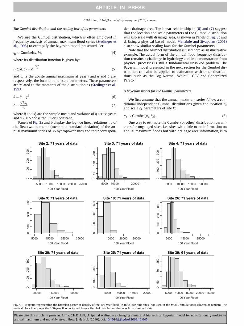
Fig. 4. Histogram representing the Bayesian posterior density of the 100-year flood (invertical black line shows the 100-year flood obtained from a Gumbel distribution that w


dent drainage area. The linear relationship in (6) and (7) suggestthat the location and scale parameters of the Gumbel distributionwill also scale with drainage area, as shown in Panels of Fig. 3c andd. Using a physical based model, Menabde and Sivapalan (2001)also show similar scaling laws for the Gumbel parameters.

Note that the Gumbel distribution is used here as an illustrativeexample. The actual form of the annual flood frequency distribu-tion remains a challenge in hydrology and its demonstration fromphysical processes is still a fundamental unsolved problem. TheBayesian model presented in the next section for the Gumbel dis-tribution can also be applied to estimation with other distribu-tions, such as the Log Normal, Weibull, GEV and GeneralizedPareto.

A bayesian model for the Gumbel parameters

We first assume that the annual maximum series follow a con-ditional independent Gumbel distributions given the location ak

and scale bk parameters of site k:

qik � Gumbelðak; bkÞ: ð8Þ

One way to estimate the Gumbel (or other) distribution param-eters for ungauged sites, i.e., sites with little or no information onannual maximum floods but with drainage area information, is to

ears of data

ar Flood

20000


100 Year Flood5000 10000 15000 20000

010

020

030

0

ears of data

ar Flood00 30000


100 Year Flood5000 15000 25000

010

020

030

0

ears of data

ar Flood0 15000 20000


100 Year Flood5000 10000 15000 20000 25000

050

150

250

m3=s) for nine sites (not used in the MCMC simulations) selected at random. Theas fit to observed data.




ARTICLE IN PRESS

obtain the first two product moments of its distribution throughsome equation that relates these distribution parameters to thedrainage area for sites with data (for instance, obtaining from Pan-els of Fig. 3a and b). These ‘‘regression” based estimates can thenbe used in (6) and (7) to obtain estimates for the location and scaleparameters at the ungaged sites. Usually, the uncertainty in theestimates of the at-site moments for the sites with records (poten-tially of unequal lengths) or in the regression vs drainage area isnot formally considered or transmitted to the subsequent estima-tion process. Also, the changes of these parameters with timedue to climate or land use are not formally integrated.

Under a Bayesian framework, we assume that the parameters in(8) follow a probability distribution, i.e., their prior distribution.Since empirical (Panels of Fig. 3c and d) as well as physical modelbased (Menabde and Sivapalan, 2001) evidence indicates that bothGumbel parameters scale with the drainage area, we assume thatthe prior distribution of location and scale parameters also followsa log–log linear relationship with respect to the drainage area:

pðlogðakÞÞ � Nða0 þ a1xðkÞ;r2aÞ ð9Þ

pðlogðbkÞÞ � Nðb0 þ b1xðkÞ;r2bÞ; ð10Þ

where k refers to streamflow gauge k and xðkÞ is the zero mean log-arithmic area, defined as xðkÞ ¼ logðAðkÞÞ � logðAÞ, where AðkÞ is thecatchment area of site k and logðAÞ represents the average of thelogarithmic of the catchment areas across all sites. The reason fora zero mean predictor is a reparameterization procedure in orderto reduce the correlation between the regression parameters in

−3 −2 −1 0 1 2

57

9

1931

x

log

(Y) r2=0.76

−3 −2 −1

57

9

1

log

(Y) r2=0.78

−3 −2 −1 0 1 2

57

9

1946

x

log

(Y) r2=0.83

−3 −2 −1

57

9

1

log

(Y) r2=0.89

−3 −2 −1 0 1 2

57

9

1961

x

log

(Y) r2=0.84

−3 −2 −1

57

9

1

log

(Y) r2=0.82

−3 −2 −1 0 1 2

57

9

1976

x

log

(Y) r2=0.73

−3 −2 −1

57

9

1

log

(Y) r2=0.86

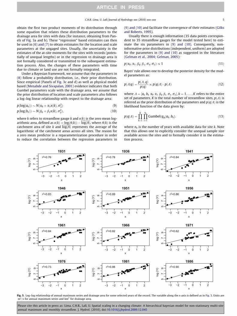
Fig. 5. Log–log relationship of annual maximum series and drainage area for some selectm3=s for annual maximum series and km2 for drainage area.


(9) and (10) and facilitate the convergence of their estimates (Gilksand Roberts, 1995).

Usually there is enough information (35 data points correspon-dent to 35 streamflow gauges for the model tested here) to esti-mate the six parameters in (9) and (10). Consequently, non-informative prior distributions (independent, uniform) are adoptedfor the parameters in (9) and (10) as suggested in the literature(Gelman et al., 2004; Gelman, 2005):

pða0;a1; b0; b1;ra;rbÞ / 1 ð11Þ

Bayes’ rule allows one to develop the posterior density for the mod-el parameters as:

pðKjqÞ ¼ pðK; qÞpðqÞ / pðqjKÞ � pðKÞ ð12Þ

where K ¼ ½ak bk a0 a1 b0 b1 ra rb�; k ¼ 1; . . . ;K refers to the entireset of parameters, K is the total number of streamflow sites, pðKÞ isreferred as the prior distribution of the parameters and pðqjKÞ is thelikelihood function of the data given by:

pðqjKÞ ¼YK

k¼1

Ynk

i¼1

Gumbelðqikjak; bkÞ: ð13Þ

where nk is the number of years with available data for site k. Notethat this allows one to explicitly consider the unequal sample sizeavailable across the sites and to formally consider it in the estima-tion process.

0 1 2

936

x−3 −2 −1 0 1 2

57

9

1941

x

log

(Y) r2=0.84

0 1 2

951

x−3 −2 −1 0 1 2

57

9

1956

x

log

(Y) r2=0.86

0 1 2

966

x−3 −2 −1 0 1 2

57

9

1971

x

log

(Y) r2=0.62

0 1 2

981

x−3 −2 −1 0 1 2

57

9

1986

x

log

(Y) r2=0.90

ed years of the record. The variable along the x-axis is defined as in Fig. 3. Units are




ARTICLE IN PRESS

Substituting the prior of the parameters as defined in (9)–(11),and the likelihood function (13) into (12), yields the joint posteriordistribution of the parameters:

pðKjqÞ /YK

k¼1

Ynk

i¼1

Gumbelðqikjak; bkÞ � NðlogðakÞja0

þ a1xðkÞ;r2aÞ � NðlogðbkÞjb0 þ b1xðkÞ;r2

bÞ ð14Þ

Eq. (14) involves the estimation of several parameters, with non-conjugate prior distributions for the Gumbel scale and locationparameters and for the regression parameters. The integral overall parameters can not be directly solved. In this case, we have toturn on to other methods. We adopt here the widely used MarkovChain Monte Carlo (MCMC) method to draw values of the set ofparameters from their posterior distribution (14). In particular, wecombine the Gibbs sampler and the Metropolis algorithm (Gelmanet al., 2004) for simulating from (14). We apply Gibbs sampler forthe regression parameters, since a closed form of the conditionalposterior distribution (normal distribution in this case) can be eas-ily obtained given the uniform prior distribution (Gelman et al.,2004) adopted. The Metropolis algorithm is used to obtain samplesfrom the conditional posterior distribution of the location and scaleparameters, since there is no closed form for this distribution. AMCMC simulation as described above is run with five chains to ver-ify the convergence of the results (or the mixing) based on themethodology suggested by Gelman et al. (2004).

In order to verify the skill of the model in reproducing the data(predictive check), 1000 simulations of the joint posterior distribu-tion of the regression parameters in (9) and (10) were drawn andapplied to nine randomly selected streamflow sites that were notused in the MCMC simulation. Fig. 4 shows the posterior distribu-tion of the 100-year flood (i.e., the 1 � 1/100 = 0.99 quantile in Eq.(5)) along with the estimates obtaining after fitting a Gumbel dis-tribution to the observed annual maximum series. A general agree-ment is obtained for all sites. The estimated 100-year flood based

φ 0

1930 1940 1950 1960

7.5

8.0

8.5

a) Interce

φ 1

1930 1940 1950 1960

0.60

0.65

0.70

0.75

b) Slope

Fig. 6. Stationary pooled estimates (horizontal dotted line) along with 95% confidence in(gray shaded region) of (a) intercept and (b) slope of the scale equation for annual max


on site data (vertical bar in Fig. 4) lies well within the distributionof the 100-year flood based on the MCMC estimates.

In the context of PUB, the model proposed here is able to predictthe (posterior) distribution rather than point estimates of any an-nual maximum statistic given only the drainage area of the unga-uged sites. Doing that, we are able to provide the uncertainty bandof our estimates (the 100-year flood in case of Fig. 4) after simulta-neously accounting for (i) the uncertainty in the Gumbel distribu-tion parameters of the sites with available data and (ii) uncertaintyfrom the scaling law regression.

Hierarchical bayesian modeling considering nonstationarity inthe scaling of annual maximum flood series

A key problem that has been highlighted recently is that anthro-pogenic climate change and land use, as well as natural climatevariability at inter-annual and decadal time scales lead to nonsta-tionarity in the probability distribution of floods and other hydro-logic variables. If these relations are temporally variable, thenreconstructing past historical data at ungaged locations becomesmuch more challenging, since the statistical relationship thatshould be used for the purpose may itself have parameters thatare changing with time. In this Section we consider the potentialimportance of this issue for the Brazilian data, and propose and ap-ply a methodology that allows for a formal consideration of thesetime varying relationships, i.e., a non-stationary model. Fig. 5shows the log–log scaling law of annual maximum series andcatchment area for selected years of the record. This motivatesthe modeling of annual maximum series through time varyingscaling coefficients, while minimizing the increase in uncertaintyof estimation in the process:

logðqikÞ � Nð/0i þ /1ixðkÞ; s2i Þ: ð15Þ

where k and i represent site and year, respectively.

1970 1980 1990 2000

pt Parameter

Year1970 1980 1990 2000

Parameter

terval (horizontal dashed lines) and average (black line) and 95% Bayesian estimatesimum series.




ARTICLE IN PRESS

The limited amount of data to estimate the regression parame-ters in (15) leads to low degrees of freedom and high uncertainty inthe estimates. For instance, Fig. 2 shows that in the beginning ofthe record (between 1930 and 1940) one had less than 60% (orabout 25 reservoirs) of the total number of hydropower sites withavailable data. In order to pool more information for estimating thetime varying parameters in (15) and consequently reduce theiruncertainty, one can assume that those parameters are drawn froma common distribution, which is represented by their long timeaverage (the distribution that would apply under stationarity),but with some additional variation that may or may not be system-atic with time. The amount of additional variation to allow is aparameter of a hierarchical model. In effect, one can think of amodel that assumes the same relationship holds across all yearsas a fully pooled regression – all years contribute in the sameway to the regression and are assumed to have the same underly-ing parameters. Conversely, if scaling parameters could be esti-mated separately for each year, then one would assume thateach year’s scaling represents a separate process. The HierarchicalBayesian model solves for the amount of variation to allow fromthe fully pooled model so that an appropriate degree of poolingacross years is allowed and departures from the underlying pooledmodel can be appropriately recognized with a quantification of theassociated uncertainty. These departures may be purely random in


Year

y

1930 1950 1970 1990

500

2000

1000

0 r=0.62

Site 2: 71 y

Y

y

1930 1950

500

2000

1000

0 r=0.70


Year

y

1930 1950 1970 1990

200

1000

5000

r=0.63

Site 13: 28

Y

y

1930 1950

500

2000

1000

0 r=0.75


Year

y

1930 1950 1970 1990

500

2000

1000

0 r=0.67

Site 31: 53

Y

y

1930 1950

200

1000

5000 r=0.67

Fig. 7. Observed annual maximum (black lines) of sites (chosen at random) that wereexpected (median) annual maximum (red lines) resulting from Bayesian simulations. Threferences to colour in this figure legend, the reader is referred to the web version of th


time due perhaps to outliers in data, or they may exhibit system-atic variation in time, in which case a specific hypothesis for theform of the nonstationarity can be formulated and explored. Ofcourse, in the process one would have an equation for each yearto apply for filling in values at ungauged locations that recognizesthe changing climate conditions that may apply to that year. Math-ematically, we can proceed by defining the following priordistribution:

/0;i

/1;i

!� N

�/0

�/1;R

!ð16Þ

where �/0 and �/1 can be considered to be the parameters that applyacross years, and R is a covariance matrix of these parameters.

For simplicity, since there is no a priori information about thevariance term in (15), we just assume a uniform prior distribution:

pðsiÞ / 1: ð17Þ

Usually there are enough data available to estimate the mean andcovariance matrix in (16), so a common choice of prior distributionscan be independent uniform priors (in the case of R, a Jefreys prior,see Gelman et al., 2004) for all parameters. However, initial analysiswith our data showed that the off diagonal elements of R and the

ears of data

ear1970 1990


Year

y

1930 1950 1970 1990

5020

010

00

r=0.38

years of data

ear1970 1990


Year

y

1930 1950 1970 1990

200

500

2000

r=0.71

years of data

ear1970 1990


Year

y

1930 1950 1970 1990

2e+0

31e

+04

5e+0

4 r=0.85

not used in the MCMC simulations versus 95% interval (gray shaded region) ande y-axis ðm3= sÞ is in the log scale for better visualization. (For interpretation of theis article.)




ARTICLE IN PRESS

variance of /1;i are relatively close to zero (order of 10�4), whichmakes MCMC convergence difficult (Gilks and Roberts, 1995). Sincefinding uniform (or non-informative) priors for such type of covari-ance matrices is still a topic of research in Bayesian statistics (seefor instance, Gilks and Roberts (1995) or the suggestion in Gelman(2005) to generalize his recently proposed prior distribution for var-iance parameters to covariance matrices), we adopt here conjugateprior distributions with hyperparameters ðK0; m0; /0; /0; k0Þ esti-mated from data:

R � Inv-Wishartm0 ðK0Þ ð18Þ�/0

�/1

��R !

� N/0

/1

;R=k0

!ð19Þ

where m0 and K0 are, respectively, the degrees of freedom and theinverse scale matrix of the inverse Wishart distribution.

Combining prior distributions and the likelihood function (15)yields the joint posterior distribution of the complete set of param-eters U:

−3 −1 0 1 2

24

68

10

MAR 1931: r2 =0.85

x

log

(y)

7.8 + 0.86 * x

−3 −1 0 1 2

24

68

10

JUN 1931: r2 =0.92

x

log

(y)

6.7 + 0.88 * x

−3 −1 0 1 2

24

68

10

MAR 1950: r2 =0.88

x

log

(y)

7.4 + 0.80 * x

−3 −1 0 1 2

24

68

10

JUN 1950: r2 =0.91

x

log

(y)

6.4 + 0.82 * x

−3 −1 0 1 2

24

68

10

MAR 1969: r2 =0.88

x

log

(y)

6.7 + 0.91 * x

−3 −1 0 1 2

24

68

10

JUN 1969: r2 =0.92

x

log

(y)

6.0 + 0.86 * x

−3 −1 0 1 2

24

68

10

MAR 1988: r2 =0.91

x

log

(y)

7.4 + 0.88 * x

−3 −1 0 1 2

24

68

10

JUN 1988: r2 =0.81

x

log

(y)

6.7 + 0.79 * x

Fig. 8. Log–log relationship of streamflow monthly series and drainage area for some selefor annual maximum series and km2 for drainage area.


pðUjqÞ /YK

k¼1

Ynk

i¼1

NðlogðqikÞj/0i þ /1ixðkÞ; s2i Þ � N

/0;i/1;i

�� /0�/1;R

� �� Inv-Wishartm0 ðRjK0Þ � N

�/0�/1

�� /0

/1;R=k0

� �: ð20Þ

Posterior samples of parameters from (20) are drawn using theGibbs sampler algorithm (Gelman et al., 2004). The posteriorparameters /0i and /1i are a weighted average of the likelihoodfunction and the prior distribution, resulting in a multivariate nor-mal distribution (Gelman et al., 2004, pp. 86). The posterior distri-butions of �/0; �/1 and R are also conjugate distributions (i.e. theyare in the same family of the prior distribution). Gelman et al.(2004, pp. 87–88) shows how to obtain those conditional posteri-ors as weighted averages of the prior distribution and likelihoodfunction.

Fig. 6 displays the Bayesian estimates (expected value of theposterior distribution) of the time varying intercept and slopeparameters along with the 95% interval. Pooled estimates (i.e. max-imum likelihood estimates using the complete data and assuming

−3 −1 0 1 2

24

68

10SEP 1931: r2 =0.90

x

log

(y)

6.4 + 0.83 * x

−3 −1 0 1 2

24

68

10

DEC 1931: r2 =0.87

x

log

(y)

7.0 + 0.78 * x

−3 −1 0 1 2

24

68

10

SEP 1950: r2 =0.91

x

log

(y)

5.8 + 0.83 * x

−3 −1 0 1 2

24

68

10

DEC 1950: r2 =0.82

x

log

(y)

7.1 + 0.84 * x

−3 −1 0 1 2

24

68

10

SEP 1969: r2 =0.93

x

log

(y)

5.5 + 0.88 * x

−3 −1 0 1 2

24

68

10

DEC 1969: r2 =0.87

x

log

(y)

6.9 + 0.86 * x

−3 −1 0 1 2

24

68

10

SEP 1988: r2 =0.91

x

log

(y)

6.0 + 0.85 * x

−3 −1 0 1 2

24

68

10

DEC 1988: r2 =0.92

x

log

(y)

6.8 + 0.86 * x

cted years and months of the record. The x-axis is as defined in Fig. 3. Units are m3=s




ARTICLE IN PRESS

stationarity of the parameters) and their 95% confidence intervalare also shown. Note that the Bayesian point estimates are oftenoutside the 95% confidence interval of the pooled estimates, whichsuggests (a) that the uncertainty of those pooled estimates isunderestimated, and/or (b) that there are systematic trends thatneed to be accounted for. Fig. 6 suggests a monotonic upwardtrend in the intercept and a monotonic downward trend in theslope from the non-stationary Bayesian estimates. In order tocheck whether or not those trends are statistically significant, theexpected values of the intercept and slope Bayesian estimates(black lines in Fig. 6) are used as point estimation values in aweighted linear fit on the time variable, where the uncertainty isaccounted by using weights defined as the inverse of the varianceof those estimates. The slopes obtained for the time regressions(0.009281 for the Bayesian intercept and �3:875� 10�4 for theBayesian slope with associated p-values 9:45� 10�6 and1:75� 10�5, respectively) suggest that both monotonic trends arestatistically significant. Hence, time invariant (i.e. constant) scalingparameters are poor estimates and the stationarity assumptionused for pooled estimates does not hold here. The significant tem-poral variations in the intercept and slope parameters suggest thatscaling law features might be influenced by the inter-annual andlonger variations in the climate patterns across the region investi-gated here. One can further build a climate trend model for theseparameters indexed to time (anthropogenic only) and/or Naturalclimate modes (e.g., and ENSO index) and estimate its parametersas part of the hierarchical Bayesian model. We do not pursue thisapproach formally here, but advocate it as a possible tool for sea-sonal forecasts using ENSO or for climate change downscaling orprojections.

In order to verify the ability of the model in reproducing the an-nual maximum flows of sites that were not included in the MCMCsimulations (out-of-sample sites), we show in Fig. 7 Bayesian sim-ulations of the annual maximum flow at nine out-of-sample siteschosen at random. Most of the observed annual maxima fall withinthe 95% Bayesian interval and agree well with expected annualmaximum resulting from the Bayesian simulations.

2 4 6

6.2

6.6

7.0

θ 0

2 4 6

0.82

0.84

0.86

0.88

θ 1

Fig. 9. Time average (lines with dots) intercept and slope of scaling law parameters for thFourier function as defined in Eqs. (25) and (26).


Hierarchical bayesian modeling of non-stationary monthlystreamflow series

Estimates of past monthly flows at ungauged sites or augmen-tation of time series at short record sites are of very interest forseveral reasons. For instance, in calibrating optimization modelsof hydro energy production one often needs monthly series of in-flow into the hydropower reservoirs within the system. The designof water reservoirs also requires estimates of past monthly flows inorder to define operational policies for water releases and storage,in particular for multi-year regularization reservoirs.

Empirical data (Fig. 8) from 36 streamflow sites in Brazil (spatiallocation displayed in Fig. 1) show strong evidences that monthlyflows also scales with drainage area for sites with similar seasonalpatterns. The scaling exponents for monthly flows with drainagearea are consistently less than one. A reviewer noted that if weconsider that the monthly flow volume V is given as the productof the average runoff R per unit area and the drainage area, A, thena slope of 1 is expected for the logðVÞ vs logðAÞ relation under theassumption that R is independent of A. Since this exponent is lessthan unity (estimated slopes typically fall in the range {0.8, 0.9}),an investigation into why R apparently decreases with A is neces-sary. It is likely that heterogeneity in rainfall or the coverage ofarea by storms decreases as the area increases, and hence the aver-age runoff produced per storm and by accumulation across storms,for monthly flow decreases a bit as the underlying area increases.The validity of this conjecture needs to be assessed. Inability to ac-cess highly detailed time series of event or even monthly rainfall toestablish spatial coverage prevented us from exploring this direc-tion. A mechanistic model could indeed be used with syntheticrainfall coverage and other variations to explore this idea.

Similarly to the model for the annual maximum as defined in(15), we can define a stochastic model for the monthly flow y:

logðyijkÞ � Nðh0ij þ h1ijxðkÞ;r2ijÞ ð21Þ

where yijk is the streamflow of site k at month j of year i.

8 10 12

a

Month

8 10 12

b

Month

e monthly flow (Eqs. (21) and (22)). The black lines show the fitting of one-harmonic




ARTICLE IN PRESS

In the first hierarchy of the model, we shrink the monthly inter-cept and slope parameters in (21) towards a common distributionacross years as was done in the previous Section for annual maxi-mum flows:

h0ij

h1ij

� �� N

�h0j

�h1j;Rj

!ð22Þ

For simplicity, we use a common approach in the literature (Gelmanet al., 2004) and define uniform prior distribution for the scaleparameters:

pðrijÞ / 1: ð23Þ

Empirical analysis (Fig. 9) also shows that the time average (acrossyears) of the intercept and slope parameters in (21) follows a well

Site 4

Time

y

1940 1960 1980 2000

100

500

2000

1000

0

r=0.94

Si

T

y

1940 1960

100

500

2000

1000

0

r=0.95

Site 30

Time

y

1940 1960 1980 2000

500

2000

1000

050

000

r=0.88

Sit

T

y

1940 1960

100

500

2000

1000

0

r=0.68

Site 39

Time

y

1940 1960 1980 2000

100

500

2000

r=0.86

Sit

T

y

1940 1960

100

500

2000

1000

0

r=0.85

Fig. 10. Posterior simulations of monthly flow of nine sites not included previously in thlines show observed data. The correlation between the expected flow from the Bayesian sin m3=s.


defined seasonal cycle. In order to maintain this seasonal behavior,one more step of shrinkage is possible:

�h0j

�h1j

!� N

h0j

h1j

; bR !: ð24Þ

Although a further stage of modeling is still possible, we estimatethe hyperparameters in (24) from data. In particular, we fit a firstFourier harmonic function to �h0j and �h1j:

h0j ¼ u00 þu01 sin2pj12

� �þu02 cos

2pj12

� �ð25Þ

h1j ¼ u10 þu11 sin2pj12

� �þu12 cos

2pj12

� �ð26Þ

where

te 6

ime1980 2000

Site 19

Time

y1940 1960 1980 2000

5020

050

020

00

r=0.63

e 33

ime1980 2000

Site 34

Time

y

1940 1960 1980 2000

5020

050

020

00 r=0.91

e 41

ime

1980 2000

Site 42

Time

y

1940 1960 1980 2000

500

2000

1000

050

000

r=0.97

e MCMC simulation. The gray shaded region shows the 95% Bayesian interval. Blackimulations and the observed flow is shown in the top left of the figure. Flow units are



2 4 6 8 10 12

100

500

2000

1000

0 Site 4

Month

y

2 4 6 8 10 12

100

500

2000

1000

0 Site 6

Month

y

2 4 6 8 10 12

5020

010

0050

00

Site 19

Month

y

2 4 6 8 10 12

500

2000

1000

0

Site 30

Month

y

2 4 6 8 10 12

100

500

2000

1000

0 Site 33

Month

y

2 4 6 8 10 12

5020

010

00

Site 34

Month

y

2 4 6 8 10 12

100

500

2000

Site 39

Month

y

2 4 6 8 10 12

100

500

2000

1000

0 Site 41

Month

y

2 4 6 8 10 12

500

2000

1000

050

000 Site 42

Month

y

Fig. 11. Observed average monthly flow (lines with dots) and expected (average) monthly flow from Bayesian simulations (black lines). The gray shaded region shows the95% Bayesian interval. Note that these sites were not used to estimate the model parameters. Flow units are in m3=s.


ARTICLE IN PRESS

u00 ¼1

12

X12

j¼1

�h0j u10 ¼1

12

X12

j¼1

�h1j

u01 ¼2

12

X12

j¼1

�h0j � sin2pj12

� �u11 ¼

212

X12

j¼1

�h1j � sin2pj12

� �

u02 ¼2

12

X12

j¼1

�h0j � cos2pj12

� �u12 ¼

212

X12

j¼1

�h1j � cos2pj12

� �:

The resulting curve is shown in Fig. 9. The associated residual var-iance is used as an estimate for bR.

For the covariance matrix Rj in (22), one could also assume aJefreys prior, since the number of parameters (2) is small (Gelmanet al., 2004). However, as is the case for the hierarchical Bayesianmodel for the annual maximum flow, the off diagonal elementsof Rj and the variance of h1ij are relatively small, which in turn slowthe MCMC convergence. Hence, we propose a conjugate prior for Rj

with hyperparameters Kj and mj estimated from data:

Rj � Inv-WishartmjðKjÞ: ð27Þ

Combining now the likelihood function (21) with the prior distribu-tions (22), (23), (24), (27), yields the posterior distribution of the en-tire set H of model parameters:


pðHjyÞ ¼YK

k¼1

Ynk

i¼1

Y12

j¼1

NðlogðyijkÞjh0ij þ h1ijxðkÞ;r2ijÞ

� N h0ij

h1ij

�� h0j�h1j

;Rj

� �� N

�h0j�h1j

�� h0j

h1j; bR !

� Inv-WishartmjðRjjKjÞ: ð28Þ

Similar procedure as done for (20) can be used here to obtain sam-ples of parameters from the posterior distribution (28). Fig. 10shows Bayesian posterior simulations (predictive check) of themonthly streamflow of nine randomly selected out-of-sample sites.For most sites, a good agreement between simulations and ob-served data is achieved, with correlations between the expectedand the observed streamflow up to 0.98. The proposed model is alsoable to reproduce the seasonality of the streamflow (Fig. 11) acrossthe out-of-sample sites.

Summary and discussion

Our objective in this paper was to illustrate how hierarchicalBayesian models could be developed to provide a formal frame-work for estimating the uncertainty in hydrologic scaling relation-ships and the potential nonstationarity due to climate or otherfactors. The process was introduced by providing a framework




ARTICLE IN PRESS

for the Bayesian estimation of the scaling relationship with drain-age area for annual maximum flows, using the Gumbel distributionas an example with Brazilian data. This model was then extendedto illustrate how time varying scaling parameters could be esti-mated and used to assess whether there are statistically significanttrends in the data. The model was then extended to considermonthly streamflow where in addition to the nonstationarityacross years, one can account for the seasonal variation in the scal-ing relationships such that monthly flows at ungauged sites couldbe reproduced over the historical period. The obvious extension ofthe modeling framework introduced to the inclusion of climatepredictors or trend informing variables and hence providing a basisfor seasonal forecasting or climate change scenario developmentwas not pursued. Work on this extension is under progress and willbe communicated separately.

The results presented clearly demonstrate how regionalizationof flow in terms of scaling parameters can be achieved in a non-sta-tionary setting with uncertainty characterization and applied tothe successful estimation of flow parameters at ungauged loca-tions. We recognize that much of the effort in recent years is fo-cused on the parameterization of highly detailed hydrologicwater balance and stimulus–response models, and relatively littleeffort continues to be expended on empirical modeling of phenom-ena and uncertainty characterization. We see these as complemen-tary approaches, and view our work as contributing directly tooperational hydrology and water resources management by pro-viding estimates of key quantities needed for design and manage-ment using the limited data sets that are typically available whilerecognizing the key issues that need to be addressed. The frame-work we present also presents a set of performance targets thatmore physically based methods need to be able to achieve if theyare to be informative even given that they typically require dra-matically higher amounts of data and processing. Similarly, interms of process understanding, the framework presented hereprovides the capacity to explore specific hypotheses and paramet-ric structures that an investigator may propose to explore thestructure of the underlying processes, e.g., rainfall or other climateor land use data could be introduced as model predictors withappropriate functional forms for the predictive relationships. Inthe limit, a dynamical Bayesian network could be considered tomodel the dynamics of flow and information transfer across thephysical network.

Acknowledgments

We would like to thank Vijay Gupta and the anonymous re-viewer for the insightful comments that greatly improved the ori-ginal manuscript.

References

Alexander, G.N., 1972. Effect of catchment area on flood magnitude. Journal ofHydrology 16, 225–240.

Becker, A., Braun, P., 1999. Disaggregation, aggregation and spatial scaling inhydrological modelling. Journal of Hydrology 217, 239–252.

Benson, M.A., 1962. Factors influencing the occurrence of floods in a humid regionof diverse terrain. Tech. Rep. 1580-B, US Geol. Surv. Water Supply Paper, 64pp.

Gelman, A., 2005. Prior distribution for variance parameters in hierarchical models.Bayesian Analysis 1 (1), 1–19.

Gelman, A., Carlin, J.B., Stern, H.S., Rubin, D.B., 2004. Bayesian Data Analysis.Chapman & Hall/CRC.

Gilks, W.R., Roberts, G.O., 1995. Strategies for improving MCMC. In: Gilks, W.R.,Richardson, S., Spiegelhalter, D. (Eds.), Markov Chain Monte Carlo in Practice:Interdisciplinary Statistics. Chapman & Hall/HRC, pp. 89–114.

Grimm, A.M., 2004. How do La Niña events disturb the summer monsoon system inBrazil? Climate Dynamics 22, 123–138.


Gupta, V.K., Dawdy, D.R., 1995. Physical interpretations of regional variations in thescaling exponents of flood quantities. Hydrological Processes 9, 347–361.

Gupta, V.K., Waymire, E., 1990. Multiscaling properties of spatial rainfall and riverflow distributions. Journal of Geophysical Research 95 (D3), 1999–2009.

Gupta, V.K., Mesa, O.J., Dawdy, D.R., 1994. Multiscaling theory of flood peaks:regional quantile analysis. Water Resources Research 30 (12), 3405–3421.

Gupta, V.K., Troutman, B.M., Dawdy, D.R., 2007. Towards a nonlinear geophysicaltheory of floods in river networks: an overview of 20 years of progress. In:Tsonis, A., Elsner, J. (Eds.), Nonlinear Dynamics in Geosciences. Springer, pp.121–151.

Jain, S., Lall, U., 2001. Floods in a changing climate: does the past represent thefuture? Water Resources Research 37 (12), 31933205.

Júnior, D.S.R., Stedinger, J.R., Martins, E.S., 2005. Bayesian generalized least squaresregression with application to log Pearson type 3 regional skew estimation.Water Resources Research 41, 1–14.

Koscielny-Bunde, E., Kantelhardt, J.W., Braun, P., Bunde, A., Havlin, S., 2006. Long-term persistence and multifractality of river runoff records: detrendedfluctuation studies. Journal of Hydrology 322, 120–137.

Kroll, C.N., Stedinger, J.R., 1998. Regional hydrologic analysis: ordinary andgeneralized least squares revisited. Water Resources Research 34 (1), 121–128.

Kwon, H.-H., Brown, C., Lall, U., 2008. Climate informed flood frequency analysis andprediction in Montana using hierarchical Bayesian modeling. GeophysicalResearch Letters 35, 1–6.

Martins, E.S., Stedinger, J.R., 2001. Historical information in a generalized maximumlikelihood framework with partial duration and annual maximum series. WaterResources Research 37 (10), 2559–2567.

Menabde, M., Sivapalan, M., 2001. Linking space-time variability of river runoff andrainfall fields: a dynamic approach. Advances in Water Resources 24, 1001–1014.

Milly, P.C.D., Betancourt, J., Falkenmark, M., Hirsch, R.M., Kundzewicz, Z.W.,Lettenmaier, D.P., Stouffer, R.J., 2008. Stationarity is dead: whither watermanagement? Science 319, 573–574.

National Research Council, 1988. Estimating Probabilities of Extreme Floods:Methods and Recommended Research. National Academy Press, Washington,DC.

Nogues-Paegle, J., Mo, K.C., 1997. Alternating wet and dry conditions over SouthAmerica during summer. Monthly Weather Review 125, 279–291.

Pandey, G.R., Nguyen, V.-T.-V., 1999. A comparative study of regression basedmethods in regional flood frequency analysis. Journal of Hydrology 225, 92–101.

Pandey, G., Lovejoy, S., Schertzer, D., 1998. Multifractal analysis of daily river flowsincluding extremes for basins of five to two million square kilometres, one dayto 75 years. Journal of Hydrology 208, 62–81.

Poveda, G., Vélez, J.I., Mesa, O.J., Cuartas, A., Barco, J., Mantilla, R.I., Mejía, J.F., Hoyos,C.D., Ramírez, J.M., Ceballos, L.I., Zuluaga, M.D., Arias, P.A., Botero, B.A., Montoya,M.I., Giraldo, J.D., Quevedo, D.I., 2007. Linking long-term water balances andstatistical scaling to estimate river flows along the drainage network ofColombia. Journal of Hydrologic Engineering 12, 4–13.

Riggs, H.C., 1973. Regional analyses of streamflow characteristics. Tech. Rep., USGeol. Surv. Techniques of Water-Resources Investigations, book 4, Chap. B3,15pp.

Ropelewski, C.F., Halpert, M.S., 1987. Global and regional scale precipitationpatterns associated with the El Niño Southern Oscillation. Monthly WeatherReview 115, 1606–1626.

Salas, J.D., Delleur, J., Yevjevich, V., Lane, W., 1980. Applied modeling of hydrologictime series. Water Resources Publications, Littleton, Colo.

Sivapalan, M., Jothityangkoon, C., Menabde, M., 2002. Linearity and nonlinearity ofbasin response as a function of scale: discussion of alternative definitions.Water Resources Research 38 (2).

Smith, J.A., 1992. Representation of basin scale in flood peak distributions. WaterResources Research 28 (11), 2993–2999.

Stedinger, J.R., Cohn, T.A., 1986. Flood frequency analysis with historical andpaleoflood information. Water Resources Research 22 (5), 785–793.

Stedinger, J.R., Tasker, G.D., 1985. Regional hydrologic analysis 1. Ordinary,weighted, and generalized least squares compared. Water Resources Research21 (o), 1421–1432.

Stedinger, J.R., Vogel, R.M., Foufoula-Georgiou, E., 1993. Frequency analysis ofextreme events. In: Maidment, D.R. (Ed.), Handbook of Hydrology. McGraw-Hill,Inc., pp. 18.1–18.66. Chapter 18.

Tasker, G.D., Stedinger, J.R., 1989. An operational GLS model for hydrologicregression. Journal of Hydrology 111, 361–375.

Thomas, D.M., Benson, M.A., 1970. Generalization of streamflow characterisitcsfrom drainage-basin characteristics. Tech. Rep., US Geol. Surv. Water SupplyPaper 1975, 55p.

Vera, C., Baez, J., Douglas, M., Emmanuel, C.B., Marengo, J., Meitin, J., Nicolini, M.,Nogues-Paegle, J., Paegle, J., Penalba, O., Salio, P., Saulo, C., Dias, M.A.S., Dias, P.S.,Zipser, E., 2006. The South American low-level jet experiment. Bulletin of theAmerican Mathematical Society 87, 63–77.

Vogel, R.M., Sankarasubramanian, A., 2000. Spatial scaling properties of annualstreamflow in the unites states. Hydrological Sciences 45 (3), 465–476.

Yue, S., Gan, T.Y., 2004. Simple scaling properties of canadian annual averagestreamflow. Advances in Water Resources 27, 481–495.



Documents

Spatial scaling in a changing climate: A hierarchical ...water.columbia.edu/files/2011/11/LimaLall2010Scaling.pdf · assistance of Ercan Kahya, Associate Editor Keywords: Hierarchical