Gschlößl, Czado:

Spatial modelling of claim frequency and claim size ininsurance

Sonderforschungsbereich 386, Paper 461 (2005)

Online unter: http://epub.ub.uni-muenchen.de/

Projektpartner

Spatial modelling of claim frequency and claim size in insurance

Susanne Gschloßl Claudia Czado ∗

December 6, 2005

Abstract

In this paper models for claim frequency and claim size in non-life insurance are con-

sidered. Both covariates and spatial random effects are included allowing the modelling of

a spatial dependency pattern. We assume a Poisson model for the number of claims, while

claim size is modelled using a Gamma distribution. However, in contrast to the usual com-

pound Poisson model going back to Lundberg (1903), we allow for dependencies between

claim size and claim frequency. Both models for the individual and average claim sizes of a

policyholder are considered. A fully Bayesian approach is followed, parameters are estimated

using Markov Chain Monte Carlo (MCMC). The issue of model comparison is thoroughly ad-

dressed. Besides the deviance information criterion suggested by Spiegelhalter et al. (2002),

the predictive model choice criterion (Gelfand and Ghosh (1998)) and proper scoring rules

(Gneiting and Raftery (2005)) based on the posterior predictive distribution are investigated.

We give an application to a comprehensive data set from a German car insurance company.

The inclusion of spatial effects significantly improves the models for both claim frequency

and claim size and also leads to more accurate predictions of the total claim sizes. Further

we quantify the significant number of claims effects on claim size.

Key words: Bayesian inference, compound Poisson model, non-life insurance, proper scoring

rules, spatial regression models,

∗Both at Center of Mathematical Sciences, Munich University of Technology, Boltzmannstr.3, D-85747 Gar-

ching, Germany, email: cczado@ma.tum.de, susanne@ma.tum.de, http://www.ma.tum.de/m4/

1

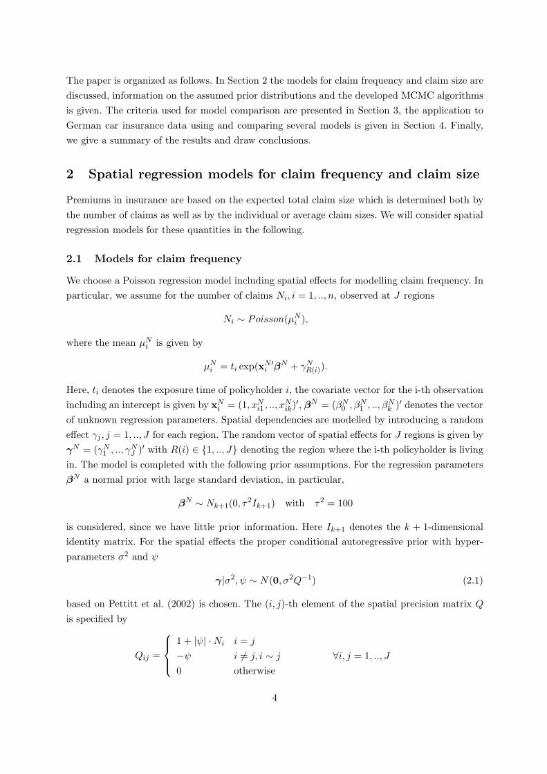
1 Introduction

In this paper statistical models for the number of claims and claim size in non-life insurance are

discussed in a Bayesian context. Based on these models the total claim size can be simulated

which is fundamental for premium calculation. In particular we consider regression models for

spatially indexed data and allow for an underlying spatial dependency pattern by the inclusion

of correlated spatial random effects. One important contribution of this paper is that we further

allow for dependencies between the number of claims and claim size. This is in contrast to the

classical compound Poisson model going back to Lundberg (1903), where independence of claim

frequency and claim size is assumed. We give an application to a comprehensive data set from

a German car insurance company and quantify the impact of number of claims effects on claim

size. Further the issue of model comparison is thoroughly addressed.

In the classical Poisson-Gamma model the number of claims is assumed to follow a Poisson

distribution and to be independent of the claim sizes which are modelled Gamma distributed.

The use of GLMs in actuarial science has been discussed by Haberman and Renshaw (1996) who

give several applications, including premium rating in non-life insurance based on models for

claim frequency and average claim size. A more detailed study of GLMs for claim frequency and

average claim sizes taking covariate information into account is given in Renshaw (1994). Taylor

(1989) and Boskov and Verrall (1994) analyse household contents insurance data incorporating

geographic information. Whereas Taylor (1989) uses spline functions, Boskov and Verrall (1994)

assume a spatial Bayesian model based on Besag et al. (1991). However, instead of performing

a separate modelling of claim frequency and claim size, in both papers adjusted loss ratios are

fitted.

Another approach, which also does not perform a separate analysis of claim size and frequency is

given by Jørgensen and de Souza (1994) and Smyth and Jørgensen (2002). They use a compound

Poisson model, which they call Tweedie’s compound Poisson model due to its association to ex-

ponential dispersion models, for analysing car insurance data. Based on the joint distribution of

the number of claims and the total claim sizes, they model the claim rate, defined by the total

costs per exposure unit, directly. The problem of premium rating taking latent structures into

account and using separate models for claim frequency and claim size has been addressed by

Dimakos and Frigessi (2002). Based on a spatial Poisson regression model and a spatial Gamma

regression model for the average claim size, they determine premiums by the product of the

expected claim frequency and the expected claim size. This approach relies on the independence

assumption of claim frequency and claim size. Here the spatial structure is modelled via an

improper Markov Random Field following Besag et al. (1991).

This paper extends the approach by Dimakos and Frigessi (2002) in several ways. We also as-

sume a spatial Poisson regression model for claim frequency. However, whereas Dimakos and

Frigessi (2002) consider only models for the average claim size per policyholder, we alternatively

assume models for the individual claim sizes of each policyholder and investigate whether this

leads to improved predictions of the total claim sizes. Further we allow for dependencies between

2

the number of claims and claim size. In particular, claim size is modelled conditionally on the

number of claims which allows us to include the observed number of claims as covariate.

We follow a fully Bayesian approach, since this allows to adjust for parameter uncertainty by

assuming the parameters to be random. Panjer and Willmot (1983) state in this context: ”The

operational actuarial interpretation is that the risk is first selected from the whole set of risks in

accordance with the risk distribution, and the performance of the selected risk is then monitored.

The statistical interpretation is essentially Bayesian.” Markov Chain Monte Carlo (MCMC) is

used for parameter estimation and thus facilitates the desired Bayesian inference.

In this paper spatial dependencies are modelled using a Gaussian conditional autoregressive

(CAR) prior introduced by Pettitt et al. (2002) for the spatial effects. CAR models are based

on the assumption that the effects of adjacent sites are similar, leading to a spatially smoothed

dependency pattern. In contrast to the widely used intrinsic CAR model introduced by Besag

and Kooperberg (1995) the spatial prior used in this paper leads to a proper joint distribution of

the spatial effects. Other proper modifications of the intrinsic CAR model have been proposed

by Sun et al. (1999) and Czado and Prokopenko (2004).

Based on the MCMC output of the models for claim frequency and the average and individual

claim sizes, respectively, we approximate the posterior predictive distribution of the total claim

sizes using simulation. We would like to emphasize again, that independence of claim size and

claim frequency is not necessary here.

Using the discussed models, we analyse a large data set from a German car insurance company.

In particular we consider policyholders with full comprehensive car insurance and claims caused

by traffic accidents. One of our main interests is to investigate whether, after adjusting for covari-

ate information, models are improved by additionally including spatial random effects. Further,

we study the impact of the observed number of claims as additional covariate for the claim size

models and quantify these effects on the expected claim sizes. Finally, we are interested, if there

is a gain in using models for individual claim sizes in contrast to models for average claim sizes,

where information is aggregated.

Models are compared using several criteria. Next to the well known deviance information cri-

terion (DIC) suggested by Spiegelhalter et al. (2002), the predictive model choice criterion

(PMCC), see for example Gelfand and Ghosh (1998), is used for comparing model fit and com-

plexity of the considered models. Further, proper scoring rules (Gneiting and Raftery (2005))

based on the posterior predictive distribution are investigated. The inclusion of spatial effects

leads to a significantly improved model fit both for claim frequency and claim size, more accurate

predictions of the total claim sizes are obtained. When spatial effects are neglected the posterior

predictive means of the total claim sizes in some regions with particular high (low) observed

total claims are estimated considerably lower (higher) than based on the spatial models. Fur-

ther, effects for the number of claims turn out to be significant for the claim size models, for

an increasing number of claims, both average and individual claim sizes tend to decrease. The

results for the average and individual claim sizes are very similar, therefore modelling of average

claim sizes seems to be sufficient.

3

The paper is organized as follows. In Section 2 the models for claim frequency and claim size are

discussed, information on the assumed prior distributions and the developed MCMC algorithms

is given. The criteria used for model comparison are presented in Section 3, the application to

German car insurance data using and comparing several models is given in Section 4. Finally,

we give a summary of the results and draw conclusions.

2 Spatial regression models for claim frequency and claim size

Premiums in insurance are based on the expected total claim size which is determined both by

the number of claims as well as by the individual or average claim sizes. We will consider spatial

regression models for these quantities in the following.

2.1 Models for claim frequency

We choose a Poisson regression model including spatial effects for modelling claim frequency. In

particular, we assume for the number of claims Ni, i = 1, .., n, observed at J regions

Ni ∼ Poisson(µNi ),

where the mean µNi is given by

µNi = ti exp(xN ′i βN + γNR(i)).

Here, ti denotes the exposure time of policyholder i, the covariate vector for the i-th observation

including an intercept is given by xNi = (1, xNi1 , .., xNik)

′, βN = (βN0 , βN1 , .., β

Nk )′ denotes the vector

of unknown regression parameters. Spatial dependencies are modelled by introducing a random

effect γj, j = 1, .., J for each region. The random vector of spatial effects for J regions is given by

γN = (γN1 , .., γNJ )′ with R(i) ∈ {1, .., J} denoting the region where the i-th policyholder is living

in. The model is completed with the following prior assumptions. For the regression parameters

βN a normal prior with large standard deviation, in particular,

βN ∼ Nk+1(0, τ2Ik+1) with τ2 = 100

is considered, since we have little prior information. Here Ik+1 denotes the k + 1-dimensional

identity matrix. For the spatial effects the proper conditional autoregressive prior with hyper-

parameters σ2 and ψ

γ|σ2, ψ ∼ N(0, σ2Q−1) (2.1)

based on Pettitt et al. (2002) is chosen. The (i, j)-th element of the spatial precision matrix Q

is specified by

Qij =

1 + |ψ| ·Ni i = j

−ψ i 6= j, i ∼ j ∀i, j = 1, .., J

0 otherwise

4

where i ∼ j denotes adjacent regions. We define regions to be neighbours if they share a common

border. The parameter ψ determines the degree of spatial dependence, for ψ = 0 the spatial

effects are independent, for increasing values of ψ an increasing spatial dependency is obtained.

For the spatial hyperparameters σ2 and ψ proper priors are assumed, in particular we choose

for σ2 the noninformative prior

σ2 ∼ IGamma(a, b) with a = 1 and b = 0.005

which is a common parameter choice for vague Gamma priors and for ψ the prior ψ ∼ 1(1+ψ)2

which is concentrated on small values for ψ close to 0. Only the hyperparameter 1σ2 can be

sampled directly from a Gamma distribution, for the remaining parameters a single component

Metropolis Hastings algorithm is implemented. We choose an independence proposal for the

spatial effects, in particular a t-distribution with 20 degrees of freedom having the same mode and

inverse curvature at the mode as the target distribution. As investigated in Gschloßl and Czado

(2005a) this proposal distribution leads to very good mixing samplers with low Monte Carlo

standard errors. For the regression parameters β and the spatial hyperparameter ψ symmetric

random walk proposal distributions are taken.

2.2 Models for claim size

It is natural for the analysis of claim size to take only observations with positive claim size into

account. We will consider both models for the individual claim sizes and the average claim size

of a policyholder. Since we aim to allow for the modelling of dependencies between the number

and the size of the claims, we consider models for the claim sizes conditionally on the number

of claims. Prior specifications will be given at the end of this section.

2.2.1 Modelling individual claim sizes

For policyholder i = 1, .., n let Sik, k = 1, ..,Ni, denote the individual claim sizes for the Ni

observed claims. In this paper we are interested in modelling claim sizes resulting from traffic

accidents in car insurance, not including IBNR (incurred but not reported) losses. These kind

of data typically have a skewed distribution, but do no contain extremely high claims which

would require the use of heavy tailed distributions like for example the Pareto distribution, see

for example Mikosch (2004). Therefore we assume a Gamma model in this paper. In particular,

we assume the individual claim sizes to be independent Gamma distributed conditionally on Ni

Sik|Ni ∼ Gamma(µSIi , v), k = 1, ..,Ni, i = 1, .., n (2.2)

with mean and variance given by

E(Sik|Ni) = µSIi and V ar(Sik|Ni) =(µSIi )2

v.

For the parameterisation used here, the density of the Gamma distribution is given by

f(sik|µSi , v) =

v

µSIi Γ(v)

(vsik

µSIi

)v−1exp

(

−vsik

µSIi

)

.

5

We consider a regression on the mean µSIi including covariates wi and spatial effects ζI for the

J geographical regions. By choosing a log link we obtain

µSIi = exp(w′iα

I + ζIR(i)), k = 1, ..,Ni, i = 1, .., n. (2.3)

Here wi = (1, wi1, .., wip)′ denotes the vector of covariates for the i-th observation including an

intercept, αI = (αI0, αI1, .., α

Ip)

′ the vector of unknown regression parameters and ζI = (ζI1 , .., ζIJ )

the vector of spatial effects which are modelled by a CAR prior based on Pettitt et al. (2002) like

in the Poisson model for claim frequency. Since we consider a model for the individual claim sizes

conditionally on the number of claims, the observed number of claims Ni may be introduced

as a covariate as well. The number of claims per policyholder observed in car insurance data

typically is very low, therefore we include Ni as a factor covariate with reference level Ni = 1.

Hence, including number of claims effects denoted by αINi=k, k = 2, ..,maxiNi, the mean µSIi

reads as follows

µSIi = exp(w′iα

I + ζIR(i)) (2.4)

= exp(

p∑

k=0

wikαIk +

maxi Ni∑

k=2

nkiαINi=k + ζIR(i)

), k = 1, ..,Ni, i = 1, .., n,

where nki =

{

1, Ni = k

0, otherwise.

Additional variability between policyholders might be modelled by replacing, the number of

claims effects αINi=k, k = 1, ..,maxiNi in (2.4) with normal distributed policyholder specific

random effects ci|Ni ∼ N(αINi=k, σ2Ni=k

) centered at αINi=kand variance σ2

Ni=kdepending on

the number of observed claims. However, this model extension did not improve the model fit for

the data considered in the application presented in Section 4 and therefore will not be further

persecuted.

2.2.2 Modelling average claim sizes

Alternatively, the average claim sizes Si, i = 1, .., n can be modelled. The average claim size Si

for policyholder i is given by

Si :=

Ni∑

k=1

Sik

Ni.

Since we assume the Sik|Ni, k = 1, ..,Ni to be independent and identically distributed, the

average claim size Si given the observed number of claims Ni is again Gamma distributed with

mean E(Si|Ni) = µSAi = µSIi and variance V ar(Si|Ni) =(µSA

i )2

Niv, that is we have

Si|Ni ∼ Gamma(µSAi ,Niv). (2.5)

Again a regression is performed on the mean µSAi , both covariates and spatial effects are taken

into account. Note, that the covariates w = (1, w1, .., wp) do not necessarily have to be the same

6

ones as for the individual claim sizes and that the estimated regression parameters and spatial

effects for the average claim size will differ from the ones for the individual claim sizes. To point

this out, we use the index A for the mean µSAi , the regression parameters αA and the spatial

effects ζA in the model for average claim sizes. With a log link we obtain the following model

µSAi = exp(w′iα

A + ζAR(i)).

Here again, number of claims effects αANi=k, k = 1, ..,maxiNi, can be included leading to

µSAi = exp(w′iα

A + ζAR(i)) (2.6)

= exp(

p∑

k=0

wikαAk +

maxi Ni∑

k=2

nkiαANi=k + ζAR(i)

), k = 1, ..,Ni, i = 1, .., n,

with nki defined as in the previous section.

Prior distributions for claim size models

Similar to the Poisson model for the number of claims we have little prior knowledge on the re-

gression parameters αI and αA in the models for individual and average claim sizes, respectively.

Therefore we assume a normal prior with large standard deviation, in particular,

αI ∼ Np+maxi Ni(0, τ2Ip+maxi Ni

), αA ∼ Np+maxi Ni(0, τ2Ip+maxi Ni

)

with τ2 = 100 which is a common choice. For the scale parameter v the gamma prior v|a, b ∼

Gamma(a, b), i.e. π(v|a, b) = ba

Γ(a)va−1 exp(−vb) with a = 1 is assumed, resulting in the condi-

tional mean and variance given by E(v|a = 1, b) = 1b

and V ar(v|a = 1, b) = 1b2

. Following a

fully Bayesian approach we also assign a noninformative gamma prior to the hyperparameter b,

in particular b|c, d ∼ Gamma(c, d), i.e. π(b|c, d) = dc

Γ(c)bc−1 exp(−bd) with c = 1 and d = 0.005,

resulting in E(b|c, d) = 200 and V ar(b|c, d) = 40000. However, the models turn out to be very

robust with respect to the prior on b, a very similar estimated posterior mean of v is obtained

when b is fixed to 0.005, which is a popular choice for a flat gamma prior.

The spatial effects are modeled using the conditional autoregressive prior (2.1), i.e.

ζl|σ2, ψ ∼ NJ(0, σ2Q−1), l = I,A,

assuming the same prior distributions for the hyperparameters σ2 and ψ as in Section 2.1. The

hyperparameter b can be sampled directly from a gamma distribution, for the regression param-

eters, the spatial effects and spatial hyperparameters a single component Metropolis Hastings

algorithm with the same proposal distributions as in the Poisson model given in Section 2.1 is

used. For the scale parameter v a symmetric random walk proposal distribution is taken.

3 Model comparison

For complex hierarchical models like those considered in this paper, the computation of Bayes

factors often used for model comparison, see for example Kass and Raftery (1995), requires

7

substantial efforts, see Han and Carlin (2001). Therefore, we consider model choice criterions

and scoring rules which can be easily computed using the available MCMC output here. In this

paper only nested models are compared, however, the criterions presented in this section also

can be used for comparing non nested models.

3.1 Deviance Information Criterion (DIC) and Predictive Model Choice Cri-

terion (PMCC)

The deviance information criterion (DIC), suggested by Spiegelhalter et al. (2002), for a proba-

bility model p(y|θ) with observed data y = (y1, .., yn) is defined by

DIC := E[D(θ|y)] + pD.

It considers both model fit as well as model complexity. The goodness-of-fit is measured by the

posterior mean of the Bayesian deviance D(θ) defined as

D(θ) = −2 log p(y|θ) + 2 log f(y)

where f(y) is some fully specified standardizing term. Model complexity is measured by the

effective number of parameters pD defined by

pD := E[D(θ|y)] −D(E[θ|y]).

According to this criterion the model with the smallest DIC is to be preferred. Using the avail-

able MCMC output both pD and DIC are easily computed by taking the posterior mean of the

deviance E[D(θ|y)] and the plug-in estimate of the deviance D(E[θ|y]). We will compute the

DIC with the standardizing term f(y) set equal to zero. An information theoretic discussion of

the DIC as criterion for posterior predictive model comparison is given in van der Linde (2005).

A related approach for model comparison is given by the predictive model choice criterion

(PMCC) considered by Laud and Ibrahim (1995) and Gelfand and Ghosh (1998). It is based

on the posterior predictive distribution given by p(yrep|y) =∫

p(yrep|θ)p(θ|y)dθ where yrep =

(yrep,1, .., yrep,n) denotes a new, replicated data set. Here yrep and y are assumed to be in-

dependent given θ. The posterior predictive distribution can be estimated by p(yrep|y) :=1R

∑Rj=1 p(y|θ

j) where θ

j, j = 1, .., R denotes the j-th MCMC iterate of θ after burnin. The

PMCC is defined by

PMCC :=

n∑

i=1

(µi − yi)2 +

n∑

i=1

σ2i , (3.7)

where µi := E(yrep,i|y) and σ2i := V ar(yrep,i|y) denote the expected value and the variance of a

replicate yrep,i of the posterior predictive distribution. Similar to the DIC, models with a smaller

value of the PMCC are preferred. While the first term∑n

i=1(µi − yi)2 gives a goodness-of-fit

measure which will decrease with increasing model complexity, the second term∑n

i=1 σ2i can be

considered as penalty term which will tend to be large both for poor and overfitted models, see

8

Gelfand and Ghosh (1998). The quantities µi and σ2i can be estimated based on the MCMC

output θj, j = 1, .., R by µi := 1

R

∑Rj=1 µi(θ

j) and σ2

i := 1R

∑Rj=1 σ

2i (θ

j), where µi(θ) and σ2

i (θ)

denote the mean and the variance of the underlying model p(y|θ) depending on the parameters θ.

When the mean µi(θ) and the variance σ2i (θ) of the model are not explicitly available, the PMCC

can be alternatively evaluated using simulation. For every MCMC iteration j = 1, .., R after

burnin, a replicated data set yjrep = (yjrep,1, .., y

jrep,n) can be simulated from p(y|θj). The mean

µi and the variance σ2i can then be estimated by the empirical counterparts µi := 1

R

∑Rj=1 y

jrep,i

and σSi := 1R−1

∑Rj=1(y

jrep− µi)

2. In the application given in Section 4 we will use the PMCC for

comparing models for individual, average and total claim sizes. Since the mean µi(θ) and the

variance σ2i (θ) are explicitly given in the models for the number of claims and for the individual

and average claim sizes, we will compute the PMCC directly using the MCMC output for these

models. The distribution of the total claim sizes however, is not available in an analytically

closed form, therefore here, the PMCC will be evaluated using simulation as described above.

3.2 Scoring rules for continuous variables

Gneiting and Raftery (2005) consider scoring rules for assessing the quality of probabilistic fore-

casts. A scoring rule assigns a numerical score based on the forecast of the predictive distribution

of a specific model and the value that was observed and can be used for comparing the pre-

dictive distribution of several models. Ideally, both calibration and sharpness of the predictive

distribution are taken into account.

Gneiting and Raftery (2005) also use scoring rules in estimation problems for assessing the opti-

mal score estimator for the unknown model parameters. Assume a parametric model Pθ := p(y|θ)

with parameters θ based on the sample y = (y1, .., yn). Then, the mean score

Sn(θ) =1

n

n∑

i=1

S(Pθ, yi)

can be taken as a goodness-of-fit measure, where S is a strictly proper scoring rule, i.e. the

highest score is obtained for the true model. For details on strictly proper and proper scoring

rules see Gneiting and Raftery (2005). Since for the true parameter vector θ0, see Gneiting and

Raftery (2005),

argmaxθSn(θ) → θ0, n→ ∞,

the optimum score estimator based on scoring rule S is given by θn = argmaxθSn(θ). We will

use scoring rules in a Bayesian context as measures for comparing models based on their posterior

predictive distribution. Gneiting and Raftery (2005) provide and discuss several scoring rules,

we will present some of the proper scoring rules for continuous variables here. In particular we

consider the logarithmic score (LS), the continuous ranked probability score (CRPS), the interval

score (IS) and a score for quantiles which we will denote as quantile score (QS). All these scores

are positively oriented, i.e. the model with the highest mean score Sn(θ) is favoured.

The logarithmic score LS is given by

LS(Pθ, yi) := log p(yrep = yi|y),

9

where p(yrep = yi|y) denotes the posterior predictive density at yrep = yi of the model under

consideration. When a sample of MCMC iterates θj, j = 1, .., R after burnin is available, an

approximation of log p(yrep = yi|y) for the i-th observation is straightforward, i.e.

ˆlog p(yrep = yi|y) :=1

R

R∑

j=1

log p(yi|θj),

where p(y|θj) denotes the density at the observed value y based on the j-th MCMC iterates. In

contrast to the logarithmic score which only considers the posterior predictive density evaluated

at the observed value, the following scoring rules take both calibration and sharpness into ac-

count.

The continuous ranked probability score CRPS for a parametric model Pθ with posterior pre-

dictive cumulative density function (cdf) F (x) :=∫ x

−∞ p(y|y)dy is defined by

CRPS(Pθ, yi) = −

∫ ∞

−∞(F (x) − 1{x ≥ yi})

2dx,

where 1{x ≥ y} takes the value 1 if x ≥ y and 0 otherwise. Hence, the CRPS can be interpreted

as the integrated squared difference between the predictive and the empirical cdf based on the

single observation yi. A graphical illustration of the CRPS is presented in Figure 3.2 when Pθ

is a normal distribution with mean θ1 and variance θ2. Here the pdf of a normal distribution

−10 0 100

0.1

0.2

0.3

0.4

−10 0 10

0

0.2

0.4

0.6

0.8

1

y=0

−10 0 10

0

0.2

0.4

0.6

0.8

1

y=2

−10 0 100

0.1

0.2

0.3

0.4

−10 0 10

0

0.2

0.4

0.6

0.8

1

y=0

−10 0 10

0

0.2

0.4

0.6

0.8

1

y=2

Figure 1: Pdf (left column with y = 0, 2 indicated as dashed lines) and cdf of a normal distribution

with mean 0 and standard deviation 1 (first row) and 4 (second row), respectively. The differences

between the cdf and the empirical cdf for two observations y = 0 (middle) and y = 2 (right) are

indicated as dashed regions.

with mean 0 and standard deviation 1 (left panel in first row) and 4 (left panel in second row)

10

respectively is plotted. The difference between the corresponding cdf and the empirical cdf for

two observations y = 0 and y = 2 is indicated in the middle and right plot of each row as

dashed regions. These plots show that the CRPS rewards sharp distributions, but also takes

into account if the observation y is close to the center or rather in the tails of the distribution.

According to Szekely (2003) the CRPS can be expressed as

CRPS(Pθ, yi) =1

2E|yrep,i − yrep,i| − E|yrep,i − yi|. (3.8)

Here yrep,i, yrep,i are independent replicates from the posterior predictive distribution p(·|y) and

the expectation is taken with respect to p(·|y). Estimation of the CRPS is again straightforward

using the available MCMC output: for j = 1, .., R simulate independently two replicated data sets

yjrep = (yjrep,1, .., y

jrep,n), y

jrep = (yjrep,1, .., y

jrep,n) based on the distribution p(y|θ

j) and estimate

the mean formula in (3.8) by E|yrep,i − y,rep,i| := 1R

∑Rj=1 |y

jrep,i − y

jrep,i| and E|yrep,i − yi| :=

1R

∑Rj=1 |y

jrep,i − yi|.

The interval score ISα is based on the (1 − α) 100 % posterior prediction interval defined

by I = [li, ui] where li and ui denote the α2 and 1 − α

2 quantile of the posterior predictive

distribution for the i-th observation. It rewards narrow prediction intervals and assigns a penalty

for observations which are not covered by the interval. The interval score is defined by

ISα(li, ui, yi) =

−2α(ui − li) − 4(li − yi) if yi ≤ li

−2α(ui − li) if li ≤ yi ≤ ui

−2α(ui − li) − 4(yi − ui) if yi ≥ ui

.

Using the available MCMC output, replicated data sets yjrep = (yjrep,1, .., y

jrep,n), j = 1, .., R, can

be simulated from which li and ui, i = 1, .., n can be determined. In order to compare models

based on prediction intervals with both moderate and large coverage, we will use α = 0.1 and

α = 0.5, respectively.

As will be seen in the application, the posterior predictive distribution of the total claim size

in car insurance typically has most of its mass at zero. In particular, zero will in general be

included in the posterior prediction intervals and the interval score will not be appropriate for

model comparison. Here one sided scores might be more interesting to investigate. Gneiting and

Raftery (2005) propose a proper scoring rule based on the quantiles rα,i at level α ∈ (0, 1) of

the predictive distribution for the i-th observation given by

S(rα,i, yi) = αs(rα,i) + (s(yi) − s(rα,i))1{yi ≤ rα,i} + h(yi)

for a nondecreasing function s and h arbitrary. We will use this score with the special choice

s(x) = x and h(x) = −αx and refer to the resulting scoring rule as quantile score QSα which is

given by

QSα(rα,i, yi) = (yi − rα,i)[1{yi≤rα,i} − α].

Analogous to the interval score, the α-quantile rα,i of the posterior predictive distribution can be

computed based on the MCMC output and evaluation of the quantile score is straightforward.

11

The predictive model choice criterion PMCC discussed in the previous section, can be expressed

as a scoring rule as well. The corresponding positively oriented score function is defined by

S(Pθ, yi) = −(E(yrep,i|y) − yi)2 − V ar(yrep,i|y).

However, this is not a proper scoring rule, see Gneiting and Raftery (2005) and should be used

with care.

4 Application

The models described in the previous section will now be used to analyse a data set from a

German car insurance company. Our main questions of interest for this application are the

followings: does the inclusion of spatial effects, after having adjusted for covariate information,

improve the models and can we observe a spatial pattern for the expected number of claims and

the expected claim sizes? Do the individual and average claim sizes of a policyholder depend

on the number of observed claims, i.e. are there significant number of claims effects for the

models for claim size? Based on the models for the number of claims and claim size, we finally

approximate the posterior predictive distribution of the total claim sizes. Here again, we are

interested, to what extent the inclusion of spatial and claim number effects influences the total

claim sizes. Should we prefer models for the individual or the average claim sizes?

4.1 Data description

The data set contains information about policyholders in Germany with full comprehensive car

insurance within the year 2000. Not all policyholders were insured during the whole year, however

the exposure time ti of each policyholder is known. Several covariates like age and gender of the

policyholder, kilometers driven per year, type of car and age of car are given in the data. The

deductible which differs between policyholders will also be included as covariate. Germany is

divided into 440 regions, for each policyholder the region he is living in is known. We analyse a

subset of these data, in particular we only consider traffic accident data for policyholders with

three types of midsized cars. The resulting data set contains about 350000 observations. There

is a very large amount of observations with no claim in the data set and the maximum number

of observed claims is only 4, see Table 1.

The histogram of the observed positive individual claim sizes in DM given in Figure 4.1 reveals

that the distribution of the claim sizes is highly skewed. The average individual claim size is

given by DM 5371.0, the largest observed claim size takes the value DM 49339.1 which is less

than 0.01 % of the sum of all individual claim sizes. Therefore, the use of a Gamma model seems

to be justified.

For an increasing number of observed claims, the average individual claim sizes decrease, see

Table 2, indicating a negative correlation between claim size and the number of claims.

12

number of claims percentage of observations

0 0.960

1 0.039

2 6.9 · 10−4

3 1.7 · 10−5

4 2.8 · 10−6

Table 1: Summary of the observed claim frequencies in the data

0 0.5 1 1.5 2 2.5 3 3.5 4 4.5 5

x 104

0

500

1000

1500

2000

2500

Figure 2: Histogram of the observed positive individual claim sizes.

4.2 Modelling claim frequency

We first address the modelling of claim frequency. In order to identify significant covariates

and interactions, the data set is analysed in Splus first using a Poisson model without spatial

effects. The obtained covariates specification is then used as a starting specification for our

MCMC algorithms. An intercept, seventeen covariates like age, gender of the policyholders or

mileage and interactions were found to be significant for explaining claim frequency. However, for

reasons of confidentiality no details about these covariates and their effects will be reported. In

order to obtain low correlations between covariates, we use centered and standardized covariates

throughout the whole application. Since Germany is divided into 440 irregular spaced regions,

440 spatial effects are introduced for the MCMC analysis. We are interested in spatial effects

after adjusting for population effects, therefore the population density in each region is included

as covariate as well. In particular the population density is considered on a logarithmic scale

which turned out to give the best fit in the initial Splus analysis.

The MCMC algorithm for the spatial Poisson regression model introduced in Section 2.1, is run

all observations Ni = 1 Ni = 2 Ni = 3 Ni = 4

mean 5371.0 5389.9 4403.8 3204.2 330.5

Table 2: Mean of the observed individual claim sizes taken over all observations and over obser-

vations with Ni = k, k = 1, 2, 3, 4 observed claims separately.

13

for 10000 iterations, a burnin of 1000 iterations is found to be sufficient after investigation of

the MCMC trace plots. We assume both a model including and without spatial effects, both

containing the same covariates, and compare them using the DIC and the PMCC. Although the

effective number of parameters pD increases from 16.0 to 98.2, the improvement in the goodness-

of-fit expressed by the posterior mean of the deviance E[D(θ|y)], leads to a lower value of the

DIC when spatial effects are included (see Table 3). This shows that, after taking the information

given by the covariates into account, there is still some unexplained spatial heterogeneity present

in the data which is captured by the spatial effects. Although the inclusion of the population

density in each region allows for geographic differences already, spatial random effects still have

a significant influence on explaining the expected number of claims. The PMCC given in the

Table 3 as well confirms these results.

γ DIC E[D(θ|y)] pD PMCC∑n

i=1(µi − yi)2

∑ni=1 σ

2i

no 122372 122356 16.0 28624 14297 14328

yes 122143 122045 98.2 28613 14280 14334

Table 3: DIC, posterior mean of the deviance D(θ|y), effective number of parameters pD and

PMCC, split in its two components, for the Poisson models for claim frequency with and without

spatial effects γ.

The left panel in the top row in Figure 3 shows a map of the estimated posterior means of

the spatial effects, ranging from -0.441 to 0.285. The corresponding posterior means of the risk

factors exp(γi) for the minimum and maximum spatial effects are given by 0.65 and 1.34. A

trend from the east to the west of Germany is visible for the spatial effects, the risk for claims

tends to be lower in the east and increases towards the south western regions. A map of the 80

% credible intervals for the spatial effects is given by the right panel. For the eastern and south

western regions significant spatial effects are present, whereas the spatial effects for the regions

in the middle of Germany do not significantly differ from zero.

4.3 Modelling the average claim size

In this section the average claim sizes Si :=∑Ni

k=1 Sik are analysed using the spatial Gamma re-

gression Model (2.5), i.e. Si|Ni ∼ Gamma(µSAi ,Niv) with mean specification (2.6). Considering

only observations with a positive number of claims, altogether 14066 observations are obtained.

Again, significant covariates and interactions are identified by analysing the data in Splus first,

assuming a Gamma model without spatial effects. An intercept and fourteen covariates includ-

ing gender, type and age of car as well as the population density in each region, modelled as

polynomial of order four, have been found to have significant influence. Further, the observed

number of claims Ni is included as covariate. Since the highest number of claims is four, the

number of claims is treated as a factor with three levels where Ni = 1 is taken as reference

level. These covariates will be taken into account when analysing the data set using MCMC.

14

number of claims

−0.441 0.285 −1 1

average claim size

−0.215 0.119 −1 1

individual claim size

−0.204 0.129 −1 1

Figure 3: Map of the estimated posterior means (left) together with map of the 80 % credi-

ble intervals (right) for the spatial effects in the Poisson (top row), average (middle row) and

individual (bottom row) claim size regression model. For grey regions, zero is included in the

credible interval, black regions indicate strictly positive, white regions strictly negative credible

intervals. 15

Therefore, including spatial and number of claims effects the mean µSAi is specified by

µSAi = exp(w′iα

A + ζAR(i)) = exp(

15∑

k=1

wikαAk + n2iα

ANi=2 + n3iα

ANi=3 + n4iα

ANi=4 + ζAR(i))

where nki =

{

1, Ni = k

0, otherwise. We consider both models with and without number of claims

effects αANi=k, k = 2, 3, 4 in the following, to quantify the influence of these effects. The MCMC

sampler for Model (2.5) including and without spatial effects and the observed number of claims

is run for 10000 iterations. Again a burnin of 1000 is found to be sufficiently large. Models are

compared using the DIC, the PMCC and some of the scoring rules given in Section 3. The

lowest value of the DIC is obtained for the model both including Ni and spatial effects (see

Table 4). Although the increase of the estimated effective number of parameters is very small

when the number of claims is included as covariate, the values of the posterior mean of the

deviance decreases by 28 and 40 in the model with and without spatial effects respectively,

indicating a significant improvement. The results for the scoring rules and the PMCC, divided

into its two components, see (3.7), are reported in Table 4 as well. The computation of the

DIC, the PMCC and the scores is based on 5000 iterations of the MCMC output, the first 5000

iterations are neglected. Note, that the computation of the interval score ISα and the continuous

ranked probability score CRPS is based on simulated data, whereas the logarithmic score LS

and the PMCC are calculated directly using the MCMC output. For the logarithmic score LS,

the interval score ISα and the CRPS the highest mean score Sn(θ) is obtained for the model

including spatial effects and number of claims effects. This confirms the significance of spatial

and number of claims effects. According to the negatively oriented PMCC the spatial models

also are to be preferred to the non-spatial ones. However, lower values of the PMCC are obtained

for the models without number of claims effects which is mainly caused by the second term of

the PMCC. Here it should be kept in mind, that the PMCC is not a proper scoring rule as noted

in Section 3.2.

A map of the posterior means and the 80 % credible intervals of the spatial effects for the model

both including spatial effects and Ni is given in the middle row in Figure 3. Similar results are

obtained for the model without Ni. The estimated posterior means of the risk factors exp(γi) for

the minimum and maximum spatial effects range from 0.81 to 1.13. Contrary to the estimated

spatial effects for claim frequency, the average claim size tends to be higher for some regions in

the east of Germany, whereas for regions in the south western part lower claim sizes are to be

expected. Again, according to the 80 % credible intervals, the spatial effects are only significant

for some regions in the east and the south west of Germany.

The estimated posterior means together with 95 % credible intervals of the number of claims

effects αANi=k, k = 2, 3, 4 are reported in Table 5. For an easier interpretation of the results we

also give the estimated posterior means of the factors exp(αANi=k), k = 2, 3, 4 which quantify the

relative risk in contrast to observations with the same covariates but only one observed claim.

Compared to a policyholder with one observed claim, the expected average claim size for an

16

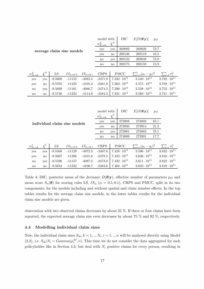
average claim size models

model with DIC E[D(θ|y)] pD

αA

Ni=kζA

yes yes 269092 269020 72.7

yes no 269136 269119 16.5

no yes 269122 269048 73.9

no no 269175 269159 15.9

αA

Ni=kζA LS ISα=0.5 ISα=0.1 CRPS PMCC

∑n

i=1(µi − yi)2

∑n

i=1 σ2i

yes yes -9.5669 -11152 -4082.4 -2471.9 7.332 · 1011 3.540 · 1011 3.792 · 1011

yes no -9.5705 -11225 -4105.2 -2481.8 7.363 · 1011 3.575 · 1011 3.788 · 1011

no yes -9.5699 -11161 -4086.7 -2474.2 7.290 · 1011 3.538 · 1011 3.752 · 1011

no no -9.5740 -11234 -4114.9 -2484.3 7.321 · 1011 3.580 · 1011 3.741 · 1011

individual claim size models

model with DIC E[D(θ|y)] pD

αI

Ni=kζI

yes yes 273888 273803 85.1

yes no 273935 273914 21.2

no yes 273961 273883 78.1

no no 274009 273991 17.7

αI

Ni=kζI LS ISα=0.5 ISα=0.1 CRPS PMCC

∑n

i=1(µi − yi)2

∑n

i=1 σ2i

yes yes -9.5568 -11129 -4072.3 -2467.6 7.428 · 1011 3.596 · 1011 3.832 · 1011

yes no -9.5607 -11206 -4101.6 -2478.5 7.452 · 1011 3.636 · 1011 3.816 · 1011

no yes -9.5596 -11157 -4087.2 -2473.8 7.432 · 1011 3.611 · 1011 3.822 · 1011

no no -9.5634 -11232 -4106.7 -2483.6 7.468 · 1011 3.650 · 1011 3.819 · 1011

Table 4: DIC, posterior mean of the deviance D(θ|y), effective number of parameters pD and

mean score Sn(θ) for scoring rules LS, ISα (α = 0.5, 0.1), CRPS and PMCC, split in its two

components, for the models including and without spatial and claim number effects. In the top

tables results for the average claim size models, in the lower tables results for the individual

claim size models are given.

observation with two observed claims decreases by about 25 %. If three or four claims have been

reported, the expected average claim size even decreases by about 75 % and 92 %, respectively.

4.4 Modelling individual claim sizes

Now, the individual claim sizes Sik, k = 1, ..,Ni, i = 1, .., n will be analysed directly using Model

(2.2), i.e. Sik|Ni ∼ Gamma(µSIi , v). This time we do not consider the data aggregated for each

policyholder like in Section 4.3, but deal with Ni positive claims for every person, resulting in

17

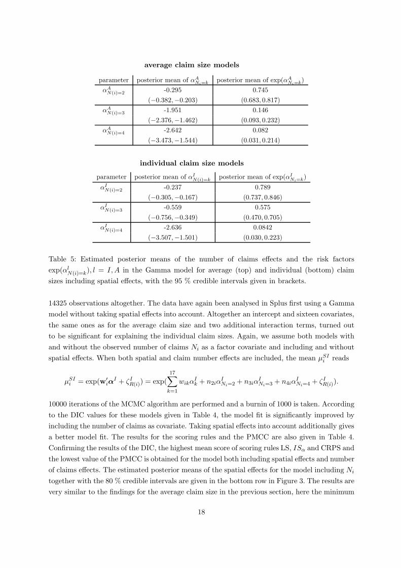
average claim size models

parameter posterior mean of αA

Ni=kposterior mean of exp(αA

Ni=k)

αA

N(i)=2 -0.295 0.745

(−0.382,−0.203) (0.683, 0.817)

αA

N(i)=3 -1.951 0.146

(−2.376,−1.462) (0.093, 0.232)

αA

N(i)=4 -2.642 0.082

(−3.473,−1.544) (0.031, 0.214)

individual claim size models

parameter posterior mean of αI

N(i)=kposterior mean of exp(αI

Ni=k)

αI

N(i)=2 -0.237 0.789

(−0.305,−0.167) (0.737, 0.846)

αI

N(i)=3 -0.559 0.575

(−0.756,−0.349) (0.470, 0.705)

αI

N(i)=4 -2.636 0.0842

(−3.507,−1.501) (0.030, 0.223)

Table 5: Estimated posterior means of the number of claims effects and the risk factors

exp(αlN(i)=k), l = I,A in the Gamma model for average (top) and individual (bottom) claim

sizes including spatial effects, with the 95 % credible intervals given in brackets.

14325 observations altogether. The data have again been analysed in Splus first using a Gamma

model without taking spatial effects into account. Altogether an intercept and sixteen covariates,

the same ones as for the average claim size and two additional interaction terms, turned out

to be significant for explaining the individual claim sizes. Again, we assume both models with

and without the observed number of claims Ni as a factor covariate and including and without

spatial effects. When both spatial and claim number effects are included, the mean µSIi reads

µSIi = exp(w′iα

I + ζIR(i)) = exp(

17∑

k=1

wikαIk + n2iα

INi=2 + n3iα

INi=3 + n4iα

INi=4 + ζIR(i)).

10000 iterations of the MCMC algorithm are performed and a burnin of 1000 is taken. According

to the DIC values for these models given in Table 4, the model fit is significantly improved by

including the number of claims as covariate. Taking spatial effects into account additionally gives

a better model fit. The results for the scoring rules and the PMCC are also given in Table 4.

Confirming the results of the DIC, the highest mean score of scoring rules LS, ISα and CRPS and

the lowest value of the PMCC is obtained for the model both including spatial effects and number

of claims effects. The estimated posterior means of the spatial effects for the model including Ni

together with the 80 % credible intervals are given in the bottom row in Figure 3. The results are

very similar to the findings for the average claim size in the previous section, here the minimum

18

and maximum posterior means of the risk factors exp(γi) are given by 0.82 and 1.14, respectively.

In Table 5 the estimated posterior means together with 95% credible intervals are reported for

the number of claims effects αINi=kand the relative risk factors exp(αINi=k

), k = 2, 3, 4, in the

model including spatial effects. The effects are significant for all levels, indicating a decrease of

the expected individual claim sizes for an increasing number of claims. Note, that in comparison

to the results for the average claim size where the factor exp(αANi=3) for observations with three

claims was estimated by 0.146, the factor exp(αINi=3) for the individual claim sizes is estimated by

0.575, resulting in a considerably lower decrease of the expected individual claim sizes. A direct

comparison of the models for average and individual claim sizes based on the DIC, the PMCC

or the scoring rules is not possible, since the average claim size models are based on aggregated

data resulting in less observations. However, qualitatively the findings are very similar, in both

approaches the best model fit is obtained when both spatial and claim number effects are taken

into account.

4.5 Posterior predictive distribution of the total claim size

The distribution of the total claim sizes is not available analytically, but can be determined

numerically using recursion formulas going back to Panjer (1981) when independence of claim

size and claim frequency is assumed. In our approach the independence assumption is violated,

however, based on the MCMC output of the models for the number of claims and claim size

the posterior predictive distribution of the total claim size can be approximated. For this inde-

pendence of claim size and the number of claims is not required. In the following we describe

how the total claim size STi =∑Ni

k=1 Sik for policyholder i = 1, .., n can be simulated based on

the MCMC output. Let βNj

, γNj ,αAj, ζAj

, αIj , ζIj, j = 1, .., R denote the MCMC draws after

burnin for the regression parameters and spatial effects of the claim frequency and claim size

models, respectively. The quantities vAj and vIj denote the MCMC draws of v in the Gamma

model for average and individual claim sizes, respectively. Then, for models based on the average

claim sizes, proceed as follows. For j = 1, .., R

• simulate N ji ∼ Poisson(µi

Nj) where µiNj := ti exp(xN ′

i βNj

+ γNj

R(i))

• if N ji = 0 set STji = 0

• otherwise simulate:

Sji ∼ Gamma(µSAji , vAjN

ji ) where µi

SAj := exp(w′iα

Aj + ζAj

R(i)) and set STji := Nji · S

ji

Based on the models for individual claim sizes, the simulation of the total claim size changes to:

for j = 1, .., R

• simulate N ji ∼ Poisson(µi

Nj) where µiNj := ti exp(xN ′

i βNj

+ γNj

R(i))

• if N ji = 0 set STji = 0

19

• otherwise simulate for k = 1, .., N ji :

Sjik ∼ Gamma(µSIji , vSj) where µi

SIj := exp(w′iα

Ij + ζIj

R(i)) and set STji :=∑N

ji

k=1 Sjik

Thus, a sample STji , j = 1, .., R of the total claim size STi is obtained by which the posterior

predictive distribution of STi can be approximated. In order to compare the simulated total

claim sizes STi based on the different models for claim size and claim frequency, we compute the

continuous ranked probability score CRPS and the predictive model choice criterion PMCC. The

DIC and the logarithmic score cannot be computed here, since they are based on the explicit

form of the total claim size distribution which is not available. The interval score will also be

omitted out of the following reasons: Due to the large amount of observations with zero claims

in our data set, the percentage of simulations with total claim size equal to zero is also very

high. Zero will be included in the (1− α) 100 % posterior predictive intervals of the total claim

sizes for α = 0.5, 0.1 for almost all observations. Therefore only observations falling above the

upper quantiles of the prediction intervals would be considered as outliers and be penalized.

Hence, the use of the interval score will not be appropriate any more. Instead we consider one-

sided quantities here like the quantiles rα at level α = 0.95, 0.99 and the number of observations

falling above these quantiles and compute the quantile score QSα described in Section 3.2 for

α = 0.95, 0.99. Both the scores as well as the PMCC are computed using 5000 simulations of

the total claim sizes STi .

The results for the simulations based on models for the average and the individual claim sizes,

reported in Tables 6 and 7, are qualitatively the same.

The PMCC favours the simulations based on the models including spatial effects for the number

of claims only, further better results are achieved when number of claims effects are taken into

account. This is caused especially by the second term of the PMCC, representing the model

variances, which are considerably lower when the number of claims is included as covariate in

the claim size models.

The mean scores for the CRPS and the quantile scores QSα, α = 0.95, 0.99, are very close for

all models, in general slightly higher scores are obtained for simulations based on a spatial

Poisson model for the number of claims. Further, the simulations based on a spatial model for

both claim frequency and claim size and including number of claims effects tend to achieve

the highest score. The size of the quantiles seems to be mainly determined by the inclusion or

neglect of spatial effects in the Poisson model for the number of claims. The quantiles at level

α = 0.95 are higher when spatial effects are included on the number of claims, reflecting a higher

model complexity. The percentage of observations falling above the 95 % quantile ranges from

3.60 % to 3.65 %, lying below the expected 5 %. This might be caused by the fact noted already

above. Since for some observations even the 95 % quantile will be only zero, a zero observation

will not be regarded as an outlier. This might be overcome by randomizing zero observations,

i.e. considering zero observations as outliers with a certain probability when the 95 % quantile

takes the value zero. The 99% quantiles in contrast, are slightly higher when no spatial Poisson

models are assumed, the percentage of outliers is close to the expected 1 %. Comparing the

20

freq size

γ ζA PMCC∑n

i=1(µi − yi)2

∑n

i=1 σ2i

with αA

Ni=k

yes yes 1.5757 · 1012 7.8032 · 1011 7.9540 · 1011

no no 1.5735 · 1012 7.8069 · 1011 7.9279 · 1011

yes no 1.5710 · 1012 7.8046 · 1011 7.9089 · 1011

no yes 1.5856 · 1012 7.8088 · 1011 8.0477 · 1011

without αA

Ni=k

yes yes 1.5960 · 1012 7.8055 · 1011 8.1541 · 1011

no no 1.5909 · 1012 7.8088 · 1011 8.1000 · 1011

yes no 1.5894 · 1012 7.8072 · 1011 8.0871 · 1011

no yes 1.6052 · 1012 7.8108 · 1011 8.2414 · 1011

freq size 95 % 99 %

γ ζA CRPS quantile outliers QS0.95 quantile outliers QS0.99

with αA

Ni=k

yes yes -212.26 476.3 3.60 % -205.2 6400.6 1.15 % -134.9

no no -212.35 456.0 3.65 % -205.7 6426.9 1.16 % -135.5

yes no -212.27 480.7 3.60 % -205.3 6393.5 1.17 % -135.4

no yes -212.36 460.0 3.65 % -205.8 6454.0 1.16 % -135.5

without αA

Ni=k

yes yes -212.30 473.6 3.60 % -205.2 6433.6 1.16 % -135.3

no no -212.30 453.8 3.65 % -205.7 6455.1 1.16 % -135.5

yes no -212.28 477.8 3.60 % -205.3 6422.6 1.17 % -135.7

no yes -212.34 456.2 3.65 % -205.9 6482.1 1.16 % -135.7

Table 6: In the upper table the PMCC, split in its two components is given for several models

for the simulated total claim sizes STi , based on models for average claim sizes. In the lower table

the mean score Sn(θ) for the CRPS, the 95 and 99 % quantiles, the percentage of observations

lying above these quantiles and the corresponding quantile mean scores QSα, α = 0.95, 0.99, are

given.

results in Tables 6 and 7, no significant difference is observed for the CRPS and the quantile

scores between the simulations based on average and individual claim sizes, respectively. When

number of claims effects are included, better values of the PMCC are obtained when models

for the average claim sizes are assumed. Without number of claims effects in contrast, the

PMCC gives a slight preference to simulations based on individual claim sizes. Hence, although

more detailed data information is available for the individual claim size models, this additional

knowledge has no significant influence on the prediction of the total claim sizes, at least when

number of claims effects are taken into account.

In Figure 4 map plots of the observed total claim sizes and the posterior predictive means

21

freq size

γ ζI PMCC∑n

i=1(µi − yi)2

∑n

i=1 σ2i

with αI

Ni=k

yes yes 1.5869 · 1012 7.8078 · 1011 8.0607 · 1011

no no 1.5830 · 1012 7.8103 · 1011 8.0196 · 1011

yes no 1.5807 · 1012 7.8091 · 1011 7.9976 · 1011

no yes 1.5960 · 1012 7.8132 · 1011 8.1473 · 1011

without αI

Ni=k

yes yes 1.5911 · 1012 7.8089 · 1011 8.1017 · 1011

no no 1.5878 · 1012 7.8120 · 1011 8.0664 · 1011

yes no 1.5865 · 1012 7.8101 · 1011 8.0550 · 1011

no yes 1.6002 · 1012 7.8141 · 1011 8.1882 · 1011

freq size 95 % 99 %

γ ζI CRPS quantile outliers QS0.95 quantile outliers QS0.99

with αA

Ni=k

yes yes -212.28 484.3 3.60 % -205.5 6442.8 1.15 % -135.0

no no -212.38 464.4 3.64 % -206.0 6469.6 1.15 % -135.3

yes no -212.35 489.3 3.60 % -205.6 6434.0 1.16 % -135.5

no yes -212.35 467.0 3.65 % -206.2 6498.1 1.16 % -135.5

without αA

Ni=k

yes yes -212.27 477.2 3.61 % -205.5 6427.2 1.16 % -135.0

no no -212.33 457.2 3.65 % -206.0 6453.8 1.16 % -135.7

yes no -212.32 481.3 3.61 % -205.6 6422.5 1.16 % -135.5

no yes -212.36 459.6 3.65 % -206.1 6481.6 1.16 % -135.6

Table 7: In the upper table the PMCC, split in its two components is given for several models for

the simulated total claim sizes STi , based on models for individual claim sizes. In the lower table

the mean score Sn(θ) for the CRPS, the 95 and 99 % quantiles, the percentage of observations

lying above these quantiles and the corresponding quantile mean scores QSα, α = 0.95, 0.99, are

given.

1R

∑Rj=1 S

Tji of the simulated total claim sizes, averaged over each region, are given. Since we

only consider the posterior predictive mean of the simulated total claim sizes, it is natural that

the map displaying the true total claim sizes shows more extreme values. Hence, for a better

visual comparison of the maps, we have built six classes for the total claim size in these plots,

assuming equal length for the four middle classes, but summarizing extremely small or high

values in broader classes. The simulations are based on the models for average claim sizes with

the number of claims included as covariate. The plots look very similar for the simulations

based on the models for the individual claim sizes. When spatial effects are included in the

Poisson model (middle row), an increasing trend from the east to the west is observable for

22

the simulated total claim sizes. The additional inclusion of spatial effects for the average claim

size leads to small changes in the very eastern and south western parts of Germany. The rough

spatial structure of the observed total claim sizes (top) is represented reasonable well for these

two models. However, if spatial effects are only included for the average claim sizes, the regions

with high observed total claim sizes in the middle and south western parts of Germany are not

detected. The same holds for the simulations based on the models without any spatial effects.

For regions in the east of Germany with rather low true total claim sizes for example, the mean

of the total claim sizes is estimated up to 1.27 times as high when no spatial effects at all are

taken into account compared to a spatial modelling of claim frequency and claim size. For one

south western region with large observed total claims in contrast, the posterior mean of the

simulated total claim size based on non spatial models is only estimated 0.69 times as large

compared to the simulations based on spatial models for claim frequency and claim size.

The estimated probabilities for the total claim sizes being equal to zero as well as density

estimates of the positive simulated total claim sizes of the policyholders in the two regions

Hannover and Lorrbach are given in Figure 5. For Hannover which is located in the northern

middle part of Germany the largest posterior mean of the spatial effect in the average claim

size model was estimated (ζA = 0.12), while in Lorrbach which is situated in the south west of

Germany the smallest effect ζA = −0.22 was observed. The true total claim size, averaged over

all policyholders in the region, is given by DM 335.0 in Hannover and DM 220.0 in Lorrbach.

The estimated posterior means of the spatial effects in the Poisson model for the number of

claims are given by γ = −0.10 in Hannover and γ = 0.29 in Lorrbach. Figure 5 shows that the

estimated probability for zero total claim sizes and the density estimates of the positive total

claim sizes notedly change when spatial effects are included to the models for claim frequency

and average claim size. In Hannover, the inclusion of spatial effects to the models for claim

frequency and the average claim size leads to a higher estimated probability of zero total claim

sizes and heavier tails for the estimated density of the positive total claim sizes. The posterior

predictive mean of the total claim sizes, averaged over all policyholders in Hannover, takes the

value 254.3 when spatial effects are included which is closer to the true total claim size than

without spatial effects where the posterior predictive mean takes the value 252.3. In Lorrbach in

contrast, the estimated probability for zero total claim sizes decreases and more mass is given to

small positive total claim sizes when spatial effects are added. Here again the posterior predictive

mean of the total claim sizes, averaged over all policyholders in Lorrbach, is closer to the true

total claim size when spatial effects are taken into account (218.4) compared to simulations

based on the non spatial models where the posterior predictive mean is estimated as 201.9.

Ideally, when the predictive quality of models is of interest, the data should not be used twice,

i.e. parameter estimation should be based on part of the data only and predictions should be

done for the remaining data. Since in this section model comparison rather than prediction was

focussed, all data were used for parameter estimation and simulation of the total claim sizes.

However, for the sake of completeness, we also fitted the Poisson models for claim frequency and

the Gamma models for the average claim size based on 75 % of the data only and simulated the

23

0 612

γ for frequency and size γ for frequency

γ for size no γ

Figure 4: Observed total claim sizes (top) and posterior predictive means of the simulated total

claim sizes based on Poisson and Gamma models for average claim sizes with and without spatial

effects. grey level classification: [0, 100), [100, 150), [150, 200), [200, 250), [200, 300), [300,∞)

24

0.9

0.91

0.92

0.93

0.94

0.95

0.96

0.97

0 0.5 1 1.5 2 2.5 3 3.5 4 4.5 5

x 104

0

1

x 10−4

Hannover with γLoerrbach with γHannover without γLoerrbach without γ

Figure 5: Estimated probabilities for zero total claim sizes (left panel) and density estimates

of the positive total claim sizes (right panel) of the policyholders in the regions Hannover and

Lorrbach based on spatial (solid lines) and non spatial (dashed lines) models for both claim

frequency and average claim size.

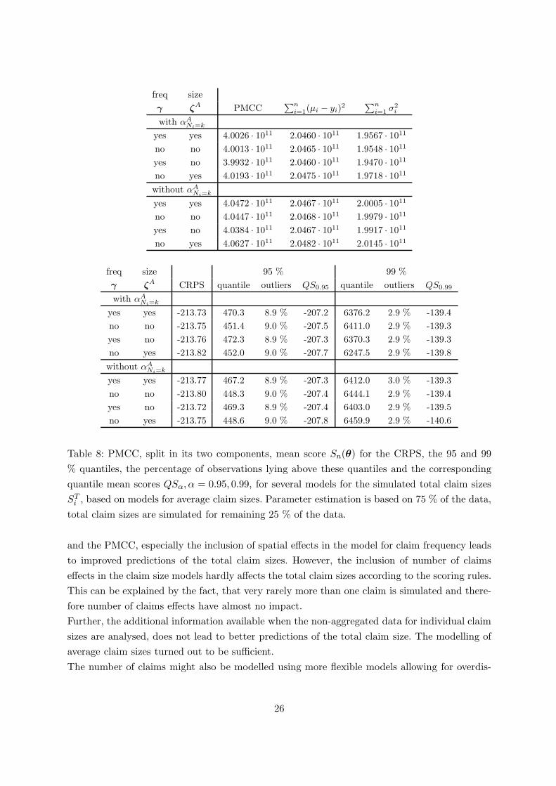
total claim sizes for the remaining 25 % of the data. Results for the PMCC, the CRPS and the

quantile scores, reported in Table 8, are qualitatively the same as observed before. The mean

scores are very close for all models, the quantile scores give a slight preference to simulations

based on a spatial Poisson model. Note, that the mean scores take lower values now compared

to the simulations based on all data. Further, about 9 % of the observations exceed the 95 %

quantile, about 2.9 % fall above the 99 % quantile. This shows, that prediction of the true total

claim sizes is worse here. However, this is to be expected, since the information given in these

25 % of the data has not been accounted for in parameter estimation.

5 Summary and conclusions

We have presented a Bayesian approach for modelling claim frequency and claim size taking both

covariates as well as spatial effects into account. In contrast to the common approach where in-

dependence of the number of claims and claim size is assumed, we do not need this assumption.

Instead, we have shown, that by including the observed number of claims as covariate for claim

size, models for claim sizes are significantly improved. If for example a policyholder caused two

or three claims, the expected average claim size decreases by about 25 and 75 %, respectively,

compared to a policyholder with only one claim.

We have considered models for both individual and average claim sizes, both models gave very

similar results in our application to car insurance data. Based on the models for claim frequency

and individual and average claim sizes, respectively, we finally approximated the posterior pre-

dictive distribution of the total claim sizes using simulation. According to several scoring rules

25

freq size

γ ζA PMCC∑n

i=1(µi − yi)2

∑n

i=1 σ2i

with αA

Ni=k

yes yes 4.0026 · 1011 2.0460 · 1011 1.9567 · 1011

no no 4.0013 · 1011 2.0465 · 1011 1.9548 · 1011

yes no 3.9932 · 1011 2.0460 · 1011 1.9470 · 1011

no yes 4.0193 · 1011 2.0475 · 1011 1.9718 · 1011

without αA

Ni=k

yes yes 4.0472 · 1011 2.0467 · 1011 2.0005 · 1011

no no 4.0447 · 1011 2.0468 · 1011 1.9979 · 1011

yes no 4.0384 · 1011 2.0467 · 1011 1.9917 · 1011

no yes 4.0627 · 1011 2.0482 · 1011 2.0145 · 1011

freq size 95 % 99 %

γ ζA CRPS quantile outliers QS0.95 quantile outliers QS0.99

with αA

Ni=k

yes yes -213.73 470.3 8.9 % -207.2 6376.2 2.9 % -139.4

no no -213.75 451.4 9.0 % -207.5 6411.0 2.9 % -139.3

yes no -213.76 472.3 8.9 % -207.3 6370.3 2.9 % -139.3

no yes -213.82 452.0 9.0 % -207.7 6247.5 2.9 % -139.8

without αA

Ni=k

yes yes -213.77 467.2 8.9 % -207.3 6412.0 3.0 % -139.3

no no -213.80 448.3 9.0 % -207.4 6444.1 2.9 % -139.4

yes no -213.72 469.3 8.9 % -207.4 6403.0 2.9 % -139.5

no yes -213.75 448.6 9.0 % -207.8 6459.9 2.9 % -140.6

Table 8: PMCC, split in its two components, mean score Sn(θ) for the CRPS, the 95 and 99

% quantiles, the percentage of observations lying above these quantiles and the corresponding

quantile mean scores QSα, α = 0.95, 0.99, for several models for the simulated total claim sizes

STi , based on models for average claim sizes. Parameter estimation is based on 75 % of the data,

total claim sizes are simulated for remaining 25 % of the data.

and the PMCC, especially the inclusion of spatial effects in the model for claim frequency leads

to improved predictions of the total claim sizes. However, the inclusion of number of claims

effects in the claim size models hardly affects the total claim sizes according to the scoring rules.

This can be explained by the fact, that very rarely more than one claim is simulated and there-

fore number of claims effects have almost no impact.

Further, the additional information available when the non-aggregated data for individual claim

sizes are analysed, does not lead to better predictions of the total claim size. The modelling of

average claim sizes turned out to be sufficient.

The number of claims might also be modelled using more flexible models allowing for overdis-

26

persion like for example the negative binomial distribution, the generalized Poisson distribution

introduced by Consul and Jain (1973) or zero inflated models, see Gschloßl and Czado (2005b)

for more details. However, for the data set analysed in this paper, the Poisson distribution turned

out to give a sufficient model fit.

Acknowledgement

We would like to thank Tilmann Gneiting for fruitful discussions and helpful suggestions on the

use of proper scoring rules. The first author is supported by a doctoral fellowship within the

Graduiertenkolleg Angewandte Algorithmische Mathematik, while the second author is supported

by Sonderforschungsbereich 386 Statistische Analyse Diskreter Strukturen, both sponsored by

the Deutsche Forschungsgemeinschaft.

References

Besag, J. and C. Kooperberg (1995). On conditional and intrinsic autoregressions.

Biometrika 82, 733–746.

Besag, J., J. York, and A. Mollie (1991). Bayesian image restoration with two applications in

spatial statistics. Ann. Inst. Statist. Math. 43, 1–59. With discussion.

Boskov, M. and R. Verrall (1994). Premium rating by geographic area using spatial models.

ASTIN Bullletin 24 (1), 131–143.

Consul, P. and G. Jain (1973). A generalization of the Poisson distribution. Technometrics 15,

791–799.

Czado, C. and S. Prokopenko (2004). Modeling transport mode decisions using hierarchi-

cal binary spatial regression models with cluster effects. Discussion paper 406, SFB 386

Statistische Analyse diskreter Strukturen. http://www.stat.uni-muenchen.de/sfb386/.

Dimakos, X. and A. Frigessi (2002). Bayesian premium rating with latent structure. Scandi-

navian Actuarial Journal (3), 162–184.

Gelfand, A. and S. Ghosh (1998). Model choice: A minimum posterior predictive loss approach.

Biometrika 85 (1), 1–11.

Gneiting, T. and A. E. Raftery (2005). Strictly proper scoring rules, prediction and estimation.

Technical report no. 463R, Department of Statistics, University of Washington.

Gschloßl, S. and C. Czado (2005a). Does a Gibbs sampler approach to spatial Poisson regres-

sion models outperform a single site MH sampler? submitted .

Gschloßl, S. and C. Czado (2005b). Modelling count data with overdispersion and spa-

tial effects. Discussion paper 412, SFB 386 Statistische Analyse diskreter Strukturen.

http://www.stat.uni-muenchen.de/sfb386/.

27

Haberman, S. and A. Renshaw (1996). Generalized linear models and actuarial science. The

Statistician 45, 407–436.

Han, C. and B. Carlin (2001). Markov chain Monte Carlo methods for computing bayes factors:

A comparative review. Journal of the American Statistical Association 96, 1122–1132.

Jørgensen, B. and M. C. P. de Souza (1994). Fitting Tweedie’s compound Poisson model to

insurance claims data. Scandinavian Actuarial Journal 1, 69–93.

Kass, R. and A. Raftery (1995). Bayes factors and model uncertainty. Journal of the American

Statistical Association 90, 773–795.

Laud, P. and J. Ibrahim (1995). Predictive model selection. Journal of the Royal Statistical

Society. Series B. Statistical Methodology 57 (1), 247–262.

Lundberg, F. (1903). Approximerad framstallning av sannolikhetsfunktionen. aterforsakring

av kollektivrisker. Akad. afhandling. almqvist och wicksell, uppsala, Almqvist och Wicksell,

Uppsala.

Mikosch, T. (2004). Non-Life Insurance Mathematics. An Introduction with Stochastic Pro-

cesses. New York: Springer.

Panjer, H. (1981). Recursive evaluation of a family of compound distributions. ASTIN Bul-

letin 11, 22–26.

Panjer, H. and G. Willmot (1983). Compound Poisson models in actuarial risk theory. Journal

of Econometrics 23, 63–76.

Pettitt, A., I. Weir, and A. Hart (2002). A conditional autoregressive Gaussian process for

irregularly spaced multivariate data with application to modelling large sets of binary

data. Statistics and Computing 12 (4), 353–367.

Renshaw, A. (1994). Modelling the claims process in the presence of covariates. ASTIN Bul-

letin 24, 265–285.

Smyth, G. K. and B. Jørgensen (2002). Fitting Tweedie’s compound Poisson model to insur-

ance claims data: dispersion modelling. ASTIN Bulletin 32 (1), 143–157.

Spiegelhalter, D., N. Best, B. Carlin, and A. van der Linde (2002). Bayesian measures of

model complexity and fit. J. R. Statist. Soc. B 64 (4), 583–640.

Sun, D., R. K. Tsutakawa, and P.L.Speckman (1999). Posterior distribution of hierarchical

models using CAR(1) distributions. Biometrika 86, 341–350.

Szekely, G. (2003). ǫ-statistics: The energy of statistical samples. Technical report no. 2003-16,

Department of Mathematics and Statistics, Bowling Green State University, Ohio.

Taylor, G. (1989). Use of spline functions for premium rating by geographic area. ASTIN

Bullletin 19 (1), 89–122.

van der Linde, A. (2005). DIC in variable selection. Statistica Neerlandica 59 (1), 45–56.

28