CS-TR-4730 June 2005

Spatial Join Techniques ∗

Edwin H. Jacox and Hanan Samet

Computer Science Department

Center for Automation Research

Institute for Advanced Computer Studies

University of Maryland

College Park, Maryland 20742

jacox@cs.umd.edu and hjs@cs.umd.edu

Keywords: spatial join, plane-sweep, external memory algorithms, spatial databases

Abstract

A variety of techniques for performing a spatial join are presented. Rather thanjust summarize the literature, this in-depth survey and analysis of spatial join algo-rithms describes distinct components of the spatial join techniques, and decomposeseach algorithm from the literature into this framework. A typical spatial join articlewill describe many components of a spatial join algorithm, such as partitioning thedata, performing internal memory spatial joins on subsets of the data, and checkingif the full polygons intersect. Rather than describe a technique in its entirety, eachtechnique is decomposed and each component is addressed in a separate section so asto compare and contrast the similar pieces of each technique. The goal of this articleis to describe algorithms within each component in detail, comparing and contrastingcompeting methods, thereby enabling further analysis and experimentation with eachcomponent and allowing for the best algorithms for a particular situation to be builtpiecemeal, or even better, allowing an optimizer to choose which algorithms to use.

∗The support of the National Science Foundation under Grants EIA-99-00268, and IIS-00-86162 is grate-fully acknowledged.

0

Table 1: Spatial join components.Section 3 Internal Memory Methods 3.1 Nested Loop Join [72]

3.2 Index Nested-Loop Join [28]3.3 Plane Sweep [9, 91]3.4 Z-Order [5, 77]

Section 4.1 External Memory Methods 4.1.1 Hierarchical Traversal [20, 36, 48, 53]Both Sets Indexed 4.1.2 Non-Hierarchical Methods [42, 54]

4.1.3 Multi-Dimensional Point Methods [96]

Section 4.2 External Memory Methods 4.2.1 Construct a Second Index [60]One Data Set Not Indexed 4.2.2 The Index as Partitioned Data [102, 69]

4.2.3 The Index as Sorted Data [8, 38]

Section 4.3 External Memory Methods 4.3.1 External Plane Sweep [50]Neither Set Indexed 4.3.2 Generic Partitioning Algorithm

4.3.6 Grid Partitioning [88, 106]4.3.7 Strip Partitioning [9]4.3.8 Size Partitioning [56, 9]4.3.9 Data Partitioning [61, 62]

Section 6 Refinement 6.1 Ordering Candidate Pairs [1]6.2 Polygon Intersection Test [91, 19]6.3 Alternate Intersection Test [19]

1 Introduction

This article presents an in-depth survey and analysis of spatial joins. A large body of diverseliterature exists on the topic of spatial joins. The goal of this article is not only to survey theliterature on spatial joins, but also to extract algorithms and techniques from the literatureand present a coherent description of the state of the art in the design of spatial join algo-rithms. Frequently, an article presents a complete framework for performing a spatial join.Instead of summarizing each complete framework individually, we decompose them intocomponents in two ways. First, if several methods are similar, then a common algorithmis extracted from the frameworks to show specifically how each framework differs from theothers. For instance, there exists several methods for performing a spatial join on R-trees[40], each using a hierarchical traversal method. From these different algorithms, we createa generic hierarchical traversal algorithm and show how each method slightly varies thegeneric algorithm (see Section 4.1.1). Thus, each method is presented in a simpler mannerthat allows it to be more thoroughly compared and contrasted to similar algorithms. Bydoing so, the strengths and weaknesses of each competing algorithm become more apparent.The various components are shown in Table 1. The second approach to deconstructing thevarious methods is to extract common issues from each and address these issues in separatesections. For instance, many of the spatial join methods for handling unindexed data mustdeal with the issue of removing duplicate results from the different stages of spatial joinprocessing. Rather than separately showing how each framework handles duplicate results,different techniques for handling duplicate results are described in a separate section (Sec-tion 4.3.5). The sections dealing with spatial join issues is shown in Table 2. Furthermore,spatial joins for specialized environments are discussed in separate sections, as listed inTable 3.

1

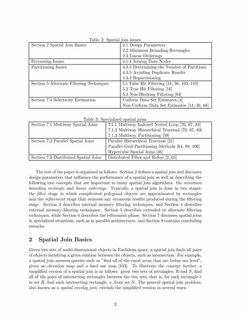
Table 2: Spatial join issues.Section 2 Spatial Join Basics 2.1 Design Parameters

2.2 Minimum Bounding Rectangles2.3 Linear Orderings

Processing Issues 4.1.4 Joining Data Nodes

Partitioning Issues 4.3.3 Determining the Number of Partitions4.3.5 Avoiding Duplicate Results4.3.4 Repartitioning

Section 5 Alternate Filtering Techniques 5.1 False Hit Filtering [18, 56, 103, 110]5.2 True Hit Filtering [16]5.3 Non-Blocking Filtering [64]

Section 7.4 Selectivity Estimation Uniform Data Set Estimates [4]Non-Uniform Data Set Estimates [14, 30, 68]

Table 3: Specialized spatial joins.Section 7.1 Multiway Spatial Joins 7.1.1 Multiway Indexed Nested Loop [70, 67, 83]

7.1.2 Multiway Hierarchical Traversal [70, 67, 83]7.1.3 Multiway Partitioning [59]

Section 7.2 Parallel Spatial Joins Parallel Hierarchical Traversal [21]Parallel Grid Partitioning Methods [64, 89, 106]Hypercube Spatial Joins [46]

Section 7.3 Distributed Spatial Joins Distributed Filter and Refine [2, 65]

The rest of the paper is organized as follows. Section 2 defines a spatial join and discussesdesign parameters that influence the performance of a spatial join as well as describing thefollowing two concepts that are important to many spatial join algorithms: the minimumbounding rectangle and linear orderings. Typically, a spatial join is done in two stages:the filter stage in which complicated polygonal objects are approximated by rectanglesand the refinement stage that removes any erroneous results produced during the filteringstage. Section 3 describes internal memory filtering techniques, and Section 4 describesexternal memory filtering techniques. Section 5 describes extended or alternate filteringtechniques, while Section 6 describes the refinement phase. Section 7 discusses spatial joinsin specialized situations, such as in parallel architectures, and Section 8 contains concludingremarks.

2 Spatial Join Basics

Given two sets of multi-dimensional objects in Euclidean space, a spatial join finds all pairsof objects satisfying a given relation between the objects, such as intersection. For example,a spatial join answers queries such as ”find all of the rural areas that are below sea level”,given an elevation map and a land use map [103]. To illustrate the concept further, asimplified version of a spatial join is as follows: given two sets of rectangles, R and S, findall of the pairs of intersecting rectangles between the two sets, that is, for each rectangle r

in set R, find each intersecting rectangle, s, from set S. The general spatial join problem,also known as a spatial overlay join, extends the simplified version in several ways:

2

1. The data sets can be objects other than rectangles such as points, lines, or polygons.

2. The data sets might have more than two dimensions.

3. The relationship between pairs of objects can be any relation between the objects,such as intersection, nearness, enclosure, or a directional relation (e.g., find all pairsof objects such that r is northwest of s [109]).

4. There might be more than two data sets in the relation (a multiway spatial join) oronly one set (a self spatial join).

Spatial joins are distinguished from a standard relational join [72] in that the join con-dition involves the multi-dimensional spatial attribute of the joined relation. This propertyprevents the use of the more sophisticated relational join algorithms. For instance, becausethe data objects are multi-dimensional, there is no ordering of the data that preserves prox-imity. Relational join techniques that rely on sorting the data, such as the sort-merge join[72], work because neighboring objects (those with the next higher and lower value) areadjacent to each other in the ordering. However, in more than one dimension, the data cannot be sorted so that this property holds. For example, in two dimensions, the left andright neighbors can be adjacent to an object in an ordering, but then the top and bottomneighbors will need to go elsewhere in the order (see Section 2.3 for a further discussion ofmulti-dimensional orderings).

Other relational join techniques are also inapplicable because the data objects mighthave extent. For example, equijoin techniques [72] (e.g. hash joins), will not work withspatial data because they rely on grouping objects with the same value, which is not possiblewhen the objects have extent. This is the same reason that the techniques will not work withintervals (extent in one dimension) or inequalities. As an example, for a one-dimensionalhash join on sets R and S, a group of objects, say G, is formed from set R and placed ina bucket. If any object g in bucket G satisfies the relation with an object from set S, thenso does every object from set G. This property does not hold for objects with extent, suchas a rectangle, because the objects can overlap each other and a disjoint grouping mightnot exist. In fact, an object from set R could potentially intersect every object from set S.Because of these two factors, not proximity preserving and extent, relational join algorithmscan not be used directly to perform a spatial join.

The computational geometry approach to solving the simplified spatial join (a two-setrectangle intersection) is to use a plane-sweep technique [91] (see Section 3.3). In order touse the plane-sweep method for a general spatial join, two problems must be overcome: thatthe objects are not rectangles and that there might be insufficient internal memory for theplane-sweep algorithm. Furthermore, calculating whether two complex objects satisfy thejoin condition, such as intersection, can be an expensive operation, and performing as fewof these operations as possible improves overall performance. To overcome these problems,a spatial join is typically performed in a two stage filter-and-refine approach [79].

In the filter-and-refine approach, the spatial join is first solved using approximations ofthe objects in the filtering stage and any incorrect results due to the approximations areremoved in the refinement stage using the full objects 1. In the filtering stage, objects are

1While the filter and refine stages can be considered two phases of one technique, Park et al. [87] proposeseparating the filter and refinement steps for query optimization so that each stage can be combined withnon-spatial queries.

3

typically approximated using minimum bounding rectangles (see Section 2.2), hereafter re-ferred to as MBR’s, which require less storage space than the full object, making processingand I/O operations less expensive 2. For example, GIS objects might be polygons, eachconsisting of thousand of points. Reading these objects in and out of memory could easilybe the dominant cost of performing a spatial join, whereas a filter-and-refine approach al-leviates this problem. Furthermore, a spatial join on rectangles presents a more tractableproblem. For smaller data sets, the filtering stage of the spatial join can be solved usinginternal memory techniques, which are described in Section 3. For larger data sets, external(secondary) memory techniques are required for the filtering stage, which are described inSection 4.

The output of the filtering stage is a list of all pairs of objects whose approximationssatisfy the join condition, which is referred to as the candidate set, and is typically rep-resented by pairs of object ids. The candidate set includes all of the desired pairs, thosewhose full objects intersect, but also includes pairs whose approximations satisfy the joincondition, but whose full objects do not. The extra pairs appear because of the inaccuracyof the object approximations (see Section 2.2). The purpose of the refinement stage is toremove the undesired pairs using the full objects, producing the final list of object pairsthat satisfy the given join condition. Refinement techniques are described in Section 6.

As mentioned, the dominant cost of a spatial join with very large objects is the I/O costof reading the large objects. Early filtering techniques were dominated by I/O costs [20].Later techniques have improved I/O performance so that it is no longer an axiom that I/Ocosts dominate the CPU costs [88]. Even though filtering reduces the I/O costs, readinglarge objects can still be the major cost of the refinement stage, which is generally moreexpensive than the filtering stage [88]. Furthermore, while the performance improvementfrom using a filter-and-refine approach might be obvious for very large objects, it remainsan open question as to whether it is the best approach for smaller, simpler objects. Asan example of an alternative approach, Zhu et al. [108, 107] have proposed methods forextending the plane-sweep algorithm (Section 3.3) to trapezoids and recti-linear polygons,thereby avoiding the need for the filter-and-refine approach.

Throughout the review of techniques, we avoid discussing experimental results. Mostof the methods in this article were shown to outperform some other method. We findmost of these experimental results to be inconclusive because they frequently use only afew data objects, the techniques are compared with one or no other technique, and theimplementations of the techniques can vary dramatically, which has a large impact onresults. Furthermore, the variety of computer hardware, software and networks used makeit difficult to compare results between methods. For these reasons, we do not discuss mostexperimental results. Nevertheless, we do point out the data set generator of Gunther etal. [37], which helps to establish a benchmark for spatial joins beyond the typical Sequoia[97] and Tiger [76] data sets. Benchmarks are an important step towards achieving the goalof repeatable and predictable algorithm performance.

Also, to simplify the discussion of the techniques, it is assumed that the data is twodimensional and that we are interested in determining pairs of intersecting objects. Both ofthese assumptions are common in the literature. The two-dimensional assumption is madebecause higher dimensional data has not been addressed in the literature in regards to spatialjoins and many of the techniques presented might not work or might not perform well inhigher dimensions. The intersection assumption is made only to simplify the discussion

2Other approximations also can be used (see Section 5).

4

and believe that this assumption does not effect the generality of the algorithms. Forexample, a nearness relation can easily be calculated by extending the size of the MBR’sso that nearness is calculated by an intersection test [57]. When appropriate, a generic joincondition is used, rather than intersection.

Furthermore, although many spatial join techniques depend on spatial indices, the dis-cussion of spatial indices is left to other work [34, 94]. Knowledge of these structures canbe crucial to a deeper understanding of many of the techniques for processing spatial data.Where appropriate, these index structures are described, but mostly the algorithms arepresented in such a way that little or no knowledge of the underlying spatial indices isrequired.

The remainder of this section discusses issues that are fundamental to the design ofspatial join algorithms. Section 2.1 discusses various design considerations and parametersthat influence the performance of spatial join algorithms. Sections 2.2 and 2.3 review MBR’sand linear orderings, respectively, which are concepts that are fundamental to many spatialjoin techniques.

2.1 Design Considerations and Parameters

Many factors contribute to the performance of a spatial join and influence the design of al-gorithms. The foremost factor, of course, is the processor speed and I/O performance. Moreimportantly for the design is the ratio of these two factors. Early spatial joins algorithmswere constrained by I/O, which dominated CPU time, and the focus of improvements wason minimizing the amount of data that needed to be read from and written to external mem-ory. As spatial join algorithms improved, experiments showed that CPU time accounted foran equal share of performance and that the algorithms were no longer I/O dominated [20].Today, algorithms need to account for both CPU performance and I/O performance. Thesetwo factors can be balanced somewhat by tuning page sizes and buffer sizes (the amount ofinternal memory available to the algorithm), two factors which also play an important rolein performance. However, as processor, I/O speeds, and internal memory sizes continueto improve, algorithms need to account for these factors and thus, tuning will always benecessary for the best performance.

The characteristics of the data sets and whether the data sets are indexed are also majorinfluences on performance. The data set sizes obviously effect overall performance, but moreimportantly is whether or not the data set fits into the available internal memory. If theentire data set does fit in internal memory, then the spatial join can be done entirely inmemory (Section 3), which can be significantly faster than using external memory methods(Section 4). One of the most confounding factors for spatial join design is the distribution ofdata. Algorithms for uniformly distributed data sets are easy to develop, but algorithms forhandling skewed data sets are significantly more complicated. A poorly designed algorithmcan thrash with skewed data sets, repeatedly reading the same data in and out of externalmemory, which severely degrades performance. These factors are mitigated if the data isindexed appropriately. If a data set is indexed, then generally, algorithms that use the indexwill be faster than those that don’t. Section 4 classifies spatial join algorithms by whetherthey assume that both data sets are indexed (Section 4.1), only one data set is indexed(Section 4.2), or neither of the data sets are indexed (Section 4.3).

How the data is stored is another factor that contributes to the design of spatial joins.Vectors (a list of vertices) are commonly used to store polygons, but raster approaches arealso used [77]. The choice of storage method for the full object mostly effects the complexity

5

of the object intersection test during the refinement stage, since an approximation of the fullobject is used during the filtering stage. This article only discusses refinement techniques forthe more common vector representation. During the filtering stage, an object is representedby an approximation and an object id or a pointer is used to access the full object. AnMBR is generally chosen as the approximation, but other approximations can also be used(see Section 5).

The environment in which the algorithm runs is also a consideration in the design ofspatial join algorithms. In a pipe-lined system [35], for instance, each stage of the spatial joinalgorithm needs to output results continuously in order for the pipe line to run efficiently.In this case, each stage is said to be non-blocking because the next stage does not needto wait for results. Unfortunately, filtering methods that sort or partition the data areblocking, although there is a method to produce some results earlier (see Section 5.3). Also,specialized algorithms can be used to improve the performance of multiway spatial joins, andmodified algorithms are required to perform spatial joins that run in parallel environmentsand distributed environments (see Section 7).

2.2 Minimum Bounding Rectangles and Approximations

y

x

(a) (b) (c)

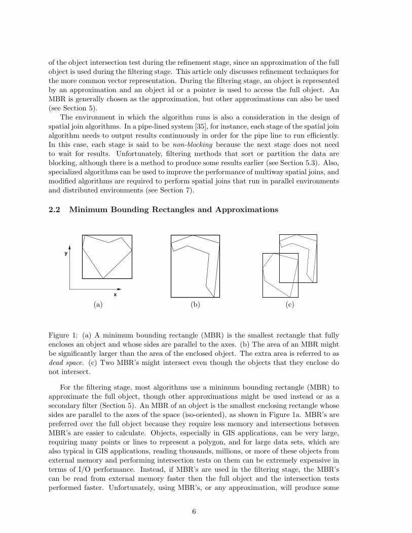
Figure 1: (a) A minimum bounding rectangle (MBR) is the smallest rectangle that fullyencloses an object and whose sides are parallel to the axes. (b) The area of an MBR mightbe significantly larger than the area of the enclosed object. The extra area is referred to asdead space. (c) Two MBR’s might intersect even though the objects that they enclose donot intersect.

For the filtering stage, most algorithms use a minimum bounding rectangle (MBR) toapproximate the full object, though other approximations might be used instead or as asecondary filter (Section 5). An MBR of an object is the smallest enclosing rectangle whosesides are parallel to the axes of the space (iso-oriented), as shown in Figure 1a. MBR’s arepreferred over the full object because they require less memory and intersections betweenMBR’s are easier to calculate. Objects, especially in GIS applications, can be very large,requiring many points or lines to represent a polygon, and for large data sets, which arealso typical in GIS applications, reading thousands, millions, or more of these objects fromexternal memory and performing intersection tests on them can be extremely expensive interms of I/O performance. Instead, if MBR’s are used in the filtering stage, the MBR’scan be read from external memory faster then the full object and the intersection testsperformed faster. Unfortunately, using MBR’s, or any approximation, will produce some

6

wrong answers. As shown in Figure 1b, an object might only occupy a fraction of its MBR,leaving a portion of dead space. Two MBR’s might intersect, but the objects they representmight not intersect, as shown in Figure 1c. This result is referred to as a false hit, whereasthe result is termed a true hit if the MBR’s intersect and the objects they represent alsointersect.

Before performing a spatial join, the MBR’s for the full objects must be calculated. Ifthe data is indexed using a spatial indexing method [34, 94], then typically the MBR’s existalready. If they do not, then a scan of the full data set is required to create the MBR’s.Forming the MBR of an object simply involves checking each corner point of the object,which is an O(n) operation for a polygonal object with n vertices.

(a) (b)

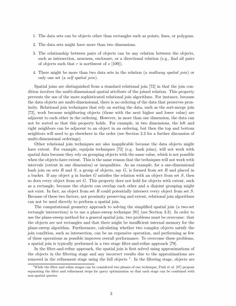
Figure 2: (a) In order to reduce dead space, an object can be approximated by two disjointrectangles. (b) However, both rectangles might intersect a second object, thereby producingduplicate results.

Use of the filter and refine approach for spatial joins was first introduced by Orenstein[79]. Orenstein was concerned that a poor approximation would degrade performance [78]and experimented with using a set of disjoint rectangles to approximate each object. Forexample, to use this representation, the object in Figure 1b is decomposed into the twoMBR’s shown in Figure 2a, improving the approximation by reducing the dead space, butalso increasing the size of the data set. While this approach improves the accuracy of thefilter stage, it also creates the need for an extra step after the filtering stage to removeduplicates from the candidate set. As shown in Figure 2, both pieces of the decomposedobject in Figure 2a might intersect the same object, as shown in Figure 2b. Both of theseintersections create a candidate pair. The duplicate results generally need to be removed formost applications and this typically should be done before the more costly refinement stagein order to avoid extra processing (see Section 4.3.5 for a discussion of duplicate removaltechniques).

Nevertheless, most algorithms use one MBR, rather than approximating an object by aset of rectangles, and rely on the refinement stage to efficiently remove false hits. However,many algorithms intentionally duplicate objects. For instance, if an algorithm creates adisjoint partition of the objects in a divide-and-conquer approach, as is done with a gridpartitioning approach (see Section 4.3.6), then each object will appear in each partitionit overlaps. Similarly, some spatial indices that can be used to perform a spatial join usedisjoint nodes and the objects again are copied into each node they overlap (e.g., the R+-tree [95]). In both cases, duplicate removal (or avoidance) techniques are required (see

7

Section 4.3.5).

2.3 Linear Orderings

a

c

d

e

b

(a)

a

c

d

e

b

(b)

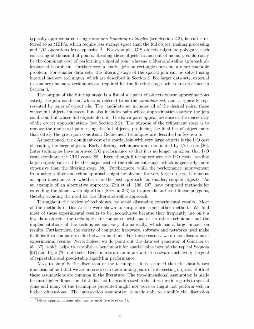
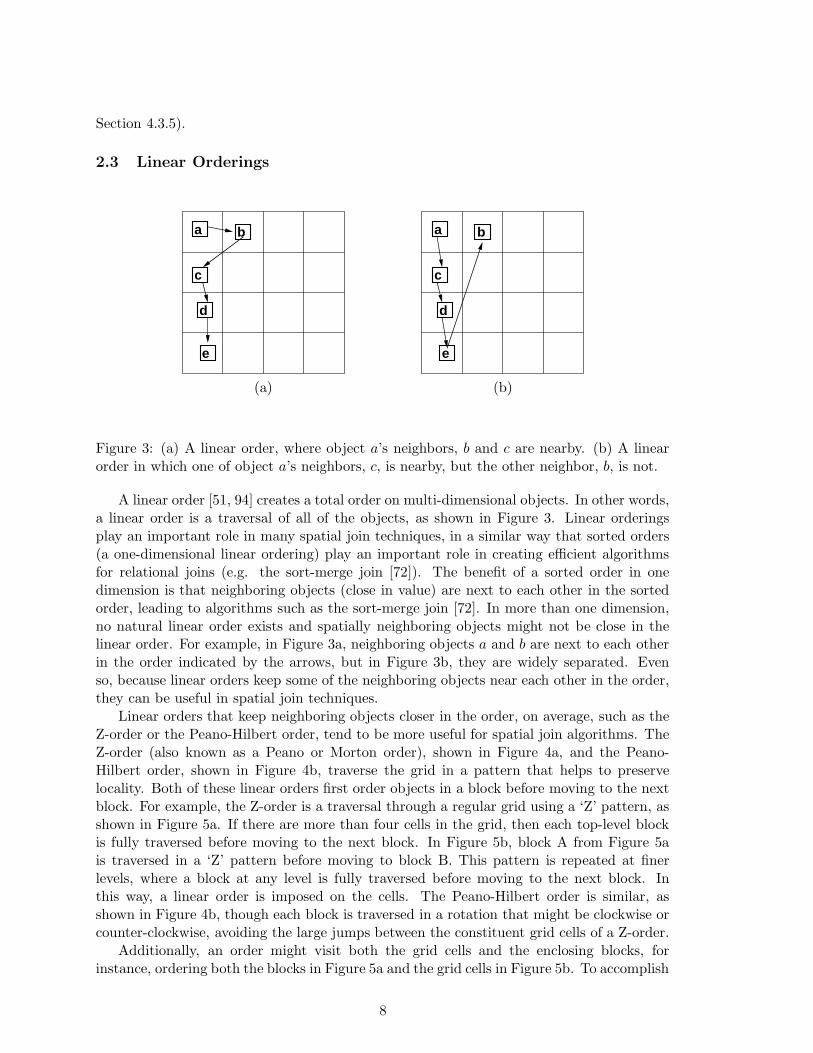
Figure 3: (a) A linear order, where object a’s neighbors, b and c are nearby. (b) A linearorder in which one of object a’s neighbors, c, is nearby, but the other neighbor, b, is not.

A linear order [51, 94] creates a total order on multi-dimensional objects. In other words,a linear order is a traversal of all of the objects, as shown in Figure 3. Linear orderingsplay an important role in many spatial join techniques, in a similar way that sorted orders(a one-dimensional linear ordering) play an important role in creating efficient algorithmsfor relational joins (e.g. the sort-merge join [72]). The benefit of a sorted order in onedimension is that neighboring objects (close in value) are next to each other in the sortedorder, leading to algorithms such as the sort-merge join [72]. In more than one dimension,no natural linear order exists and spatially neighboring objects might not be close in thelinear order. For example, in Figure 3a, neighboring objects a and b are next to each otherin the order indicated by the arrows, but in Figure 3b, they are widely separated. Evenso, because linear orders keep some of the neighboring objects near each other in the order,they can be useful in spatial join techniques.

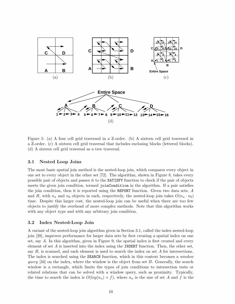
Linear orders that keep neighboring objects closer in the order, on average, such as theZ-order or the Peano-Hilbert order, tend to be more useful for spatial join algorithms. TheZ-order (also known as a Peano or Morton order), shown in Figure 4a, and the Peano-Hilbert order, shown in Figure 4b, traverse the grid in a pattern that helps to preservelocality. Both of these linear orders first order objects in a block before moving to the nextblock. For example, the Z-order is a traversal through a regular grid using a ‘Z’ pattern, asshown in Figure 5a. If there are more than four cells in the grid, then each top-level blockis fully traversed before moving to the next block. In Figure 5b, block A from Figure 5ais traversed in a ‘Z’ pattern before moving to block B. This pattern is repeated at finerlevels, where a block at any level is fully traversed before moving to the next block. Inthis way, a linear order is imposed on the cells. The Peano-Hilbert order is similar, asshown in Figure 4b, though each block is traversed in a rotation that might be clockwise orcounter-clockwise, avoiding the large jumps between the constituent grid cells of a Z-order.

Additionally, an order might visit both the grid cells and the enclosing blocks, forinstance, ordering both the blocks in Figure 5a and the grid cells in Figure 5b. To accomplish

8

(a) (b)

Figure 4: (a) Z-Order (Peano order) and (b) Peano-Hilbert order.

this order, one convention is to visit enclosing regions (the blocks in Figure 5a) before visitingsmaller regions (the cells in Figure 5b), as shown in Figure 5c, which also includes the toplevel cell (the enclosing space) in the ordering. In essence, this a hierarchical traversal ofthe nodes, as shown in Figure 5d.

To traverse points in a linear order, the grid cells can be made small enough such thateach point is in its own grid cell. To traverse objects in a linear order, either a point on theobjects, such as the centroid, is used to represent each object or the objects are assigned tothe smallest enclosing block or grid cell, which is similar to creating an MBR for the object,but with more dead space, as shown in Figure 6. Note that an object, no matter how small,that intersects the center point will always be in the top level cell (root space), as shownin Figure 7. Some algorithms can take advantage of the regular structure of the enclosingcells, but at the price of more false hits due to the increased dead space (see Sections 3.4and 4.3.8).

3 The Filtering Stage – Internal Memory

During the filtering stage, a spatial join is performed on approximations of the objects. Thissection describes techniques for performing a spatial join without using external memory,that is, no data is written to external memory. If there is insufficient internal memory toprocess a spatial join entirely in memory, then external memory must be used to store allor portions of the data sets during processing (see Section 4). Even so, at some point, mostexternal memory spatial join algorithms reduce the size of the problem and process subsetsof the data using internal memory techniques.

Section 3.1 first describes the brute force nested-loop join. Next, Section 3.2 describesthe related index nested-loop join, which is presented as an internal memory method eventhough it can be used as an external memory algorithm if the indices are stored in externalmemory. Two more sophisticated approaches are also described: the plane-sweep algorithm,rooted in computational geometry, in Section 3.3, and a variant of the plane-sweep that usesa linear ordering of the data, in Section 3.4.

9

A B

C D

(a)

A B

C D

(b)

A

B

C D

Entire Space

1 2

3 4

5 6

7 8

9 10

11 12

13 14

15 16

(c)

A

Entire Space

1 2 3 4

B

5 6 7 8

C

9 10 11 12

D

13 14 15 16

(d)

Figure 5: (a) A four cell grid traversed in a Z-order. (b) A sixteen cell grid traversed ina Z-order. (c) A sixteen cell grid traversal that includes enclosing blocks (lettered blocks).(d) A sixteen cell grid traversal as a tree traversal.

3.1 Nested Loop Joins

The most basic spatial join method is the nested-loop join, which compares every object inone set to every object in the other set [72]. The algorithm, shown in Figure 8, takes everypossible pair of objects and passes it to the SATISFY function to check if the pair of objectsmeets the given join condition, termed joinCondition in the algorithm. If a pair satisfiesthe join condition, then it is reported using the REPORT function. Given two data sets, A

and B, with na and nb objects in each, respectively, the nested-loop join takes O(na · nb)time. Despite this larger cost, the nested-loop join can be useful when there are too fewobjects to justify the overhead of more complex methods. Note that this algorithm workswith any object type and with any arbitrary join condition.

3.2 Index Nested-Loop Join

A variant of the nested-loop join algorithm given in Section 3.1, called the index nested-loopjoin [28], improves performance for larger data sets by first creating a spatial index on oneset, say A. In this algorithm, given in Figure 9, the spatial index is first created and everyelement of set A is inserted into the index using the INSERT function. Then, the other set,say B, is scanned, and each element is used to search the index on set A for intersections.The index is searched using the SEARCH function, which in this context becomes a windowquery [34] on the index, where the window is the object from set B. Generally, the searchwindow is a rectangle, which limits the types of join conditions to intersection tests orrelated relations that can be solved with a window query, such as proximity. Typically,the time to search the index is O(log(na) + f), where na is the size of set A and f is the

10

r

s

t

A B

DC

1

3 4

2 5

7

6

8

13 14

1615

10

1211

9

Figure 6: In a linear ordering, objects can be assigned to the smallest enclosing block orgrid cell. Object r is assigned to the root space since it is not within any block. Object s

is assigned to the lower right block, B, and object t is assigned to cell 14.

Figure 7: An object overlapping the center point, no matter how small, will be assigned tothe top level, which is the entire space.

number of intersections found. In theory, an object could intersect every object in the index,creating an O(n) search time. In practice though, the number of intersections is small andthe running time of the entire algorithm is O((na+nb) ·log(na)+f), which includes the timeto construct the index, which is typically O(na · log(na)). Since all of set A is inserted first,more efficient static indices and bulk-loading techniques [45, 101] can be used to improvethe construction time and the performance of the index.

The index nested-loop algorithm can be executed entirely in memory, using in memoryindices, and is useful as a component in other spatial join algorithms (see Section 4). Thealgorithm can also be used as a stand alone external memory spatial join algorithm byusing external memory indices, which allows the algorithm to process larger data sets. Forinstance, Becker et al. [13] used grid files [75] as the index and Henrich and Moller [43]used an LSD tree [44] as the index. However, more sophisticated methods exist for usingan external spatial index to perform a spatial join (see Section 4).

11

procedure NESTED_LOOP_JOIN(setA, setB, joinCondition);

begin

for each a ∈ setA

for each b ∈ SetB

if SATISFIED(a, b, joinCondition) then

REPORT(a, b);

end if;

next b;

next a;

end;

Figure 8: The basic nested loop join with running time O(na · nb), for data sets of size na

and nb.

procedure INDEX_NESTED_LOOP_JOIN(setA, setB);

begin

spatialIndex←CREATE_SPATIAL_INDEX(setA);

for each a ∈ setA

spatialIndex.INSERT(a)

end for each;

for each b ∈ setB

searchResults←spatialIndex.SEARCH(b)

REPORT(searchResults)

end for each;

end;

Figure 9: An index nested-loop join improves the performance of the spatial join to O((na+nb) · log(na) + f), assuming search times of the index are O(log(na) + f), where f is thenumber of intersections found, na is the size of the indexed data set, and nb is the size ofthe unindexed data set.

3.3 Plane Sweep

A two-dimensional plane-sweep [91] of a set of iso-oriented rectangles finds all of the rect-angles that intersect. The algorithm has two passes. The first pass sorts the rectangles inascending order on the basis of their left sides (i.e., x coordinate values) and forms a list.The second pass sweeps a vertical scan line through the sorted list from left to right, haltingat each one of these points, say p. At any instant, all rectangles that intersect the scan lineare considered active and are the only ones whose intersection needs to be checked with therectangle associated with p. This means that each time the sweep line halts, a rectanglebecomes active, causing it to be inserted into the set of active rectangles, and any rectanglesentirely to the left of the scan line are removed from the set of active rectangles 3. Thus,the key to the algorithm is its ability to keep track of the active rectangles (actually, justtheir vertical sides), as well as performing the actual intersection test.

To keep track of the active rectangles, the plane-sweep algorithm uses a structure (re-

3A variant of the plane-sweep algorithm also stops at the right sides of each rectangle, which also mustbe included in the original sorted list, and removes that rectangle from the active set.

12

procedure PLANE_SWEEP(setA, setB);

begin

listA←SORT_BY_LEFT_SIDE( setA );

listB←SORT_BY_LEFT_SIDE( setB );

sweepStructureA←CREATE_SWEEP_STRUCTURE();

sweepStructureB←CREATE_SWEEP_STRUCTURE();

while NOT listA.END() OR NOT listB.END() do

/* get left most rectangle from the two lists */if listA.FIRST() < listB.FIRST() then

sweepStructureA.INSERT(listA.FIRST());

sweepStructureB.REMOVE_INACTIVE(listA.FIRST());

sweepStructureB.SEARCH(listA.FIRST());

listA.NEXT();

else

sweepStructureB.INSERT(listB.FIRST());

sweepStructureA.REMOVE_INACTIVE(listB.FIRST());

sweepStructureA.SEARCH(listB.FIRST());

listB.NEXT();

end if;

end loop;

end;

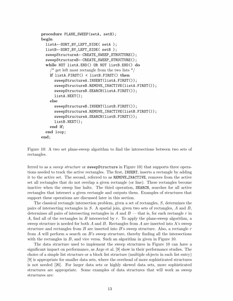
Figure 10: A two set plane-sweep algorithm to find the intersections between two sets ofrectangles.

ferred to as a sweep structure or sweepStructure in Figure 10) that supports three opera-tions needed to track the active rectangles. The first, INSERT, inserts a rectangle by addingit to the active set. The second, referred to as REMOVE INACTIVE, removes from the activeset all rectangles that do not overlap a given rectangle (or line). These rectangles becomeinactive when the sweep line halts. The third operation, SEARCH, searches for all activerectangles that intersect a given rectangle and outputs them. Examples of structures thatsupport these operations are discussed later in this section.

The classical rectangle intersection problem, given a set of rectangles, S, determines thepairs of intersecting rectangles in S. A spatial join, given two sets of rectangles, A and B,determines all pairs of intersecting rectangles in A and B — that is, for each rectangle r inA, find all of the rectangles in B intersected by r. To apply the plane-sweep algorithm, asweep structure is needed for both A and B. Rectangles from A are inserted into A’s sweepstructure and rectangles from B are inserted into B’s sweep structure. Also, a rectangle r

from A will perform a search on B’s sweep structure, thereby finding all the intersectionswith the rectangles in B, and vice versa. Such an algorithm in given in Figure 10.

The data structure used to implement the sweep structures in Figure 10 can have asignificant impact on performance, as Arge et al. [9] show in their performance studies. Thechoice of a simple list structure or a block list structure (multiple objects in each list entry)[9] is appropriate for smaller data sets, where the overhead of more sophisticated structuresis not needed [26]. For larger data sets or highly skewed data sets, more sophisticatedstructures are appropriate. Some examples of data structures that will work as sweepstructures are:

13

1. A simple linked list [23].

2. Interval tries [55], as used by Dittrich and Seeger [26].

3. A dynamic segment tree [23].

4. An interval tree [27] with a skip list [92], as described by Hanson [41] and used byArge et al. [9].

Except for the linked list implementation, the search operation on the sweep structure isO(log(n)), where n is the size of the combined data sets (na + nb), giving a running timefor the plane-sweep algorithm of O(n · log(n)), which includes the initial sort of the data.

Arge et al. [9] modify the plane-sweep algorithm slightly to dramatically increase thesize of data sets that can be processed without resorting to external memory with a tech-nique they call distribution sweeping. The traditional version of the plane-sweep algorithmassumes that all of the data is in internal memory. If the data is in external memory, thenthe entire data set is first read into internal memory before performing the plane sweep.Arge et al. [9] observed that only the data in the sweep structures needs to be kept in in-ternal memory. If the data is in external memory and sorted, then each object can be readone at time from external memory, inserted into the sweep structure, and then purged frommemory when it is deleted from the sweep structure. In this way, only the data intersectingthe sweep line needs to be kept in memory, reducing the internal memory requirements ofthe algorithm and increasing the size of data sets that can be processed without resortingto more sophisticated spatial join techniques. A rough calculation estimates that a typicaldata set will have O(

√n) objects intersecting the sweep line [81], meaning that data sets

of size O(m2), can be processed, where m is the number of objects that can fit in internalmemory. The plane-sweep technique can also be extended to process data sets of any sizeby using external memory (see Section 4.3.1).

3.4 Z-Order Methods

The plane-sweep method described in Section 3.3 only uses input sorted in one dimension,but can be adapted to use more than one dimension using a more general linear orderingthat sorts the points using multiple dimensions (see Section 2.3). Thus, instead of a sweepline, a point or grid cell is swept over the data space, creating an active border [5, 25]. Sincefewer objects will intersect a point than will intersect a line, the sweep structure will bekept smaller, decreasing search times and the amount of internal memory needed. However,since the enclosing cells used for a linear ordering are bigger than MBR’s, as shown inFigure 6, the number of objects in the sweep structure will increase, thereby offsetting someof the benefit. Orenstein [77] first used a variation of the Z-order method in his work onspatial joins. This section shows how to adapt the plane-sweep method to use a Z-order (aPeano-Hilbert order would work as well) and relates the algorithm to Orenstein’s work.

The Z-order algorithm is nearly identical to the plane-sweep algorithm, shown in Fig-ure 10, and this section only describes the two minor modifications needed for the Z-orderalgorithm, rather than listing the entire algorithm. First, the objects from both sets areassigned to Z-order grid cells (see Section 2.3), and second, are then sorted in Z-order ratherthan one-dimensionally. The remainder of the Z-order algorithm, which consists of creatingthe sweep structures and the while loop, is identical to the plane-sweep algorithm, shown inFigure 10. In this case, the active set, instead of being the objects that intersect the sweepline, are the enclosing cells of the objects that intersect the current Z-order grid cell. Since

14

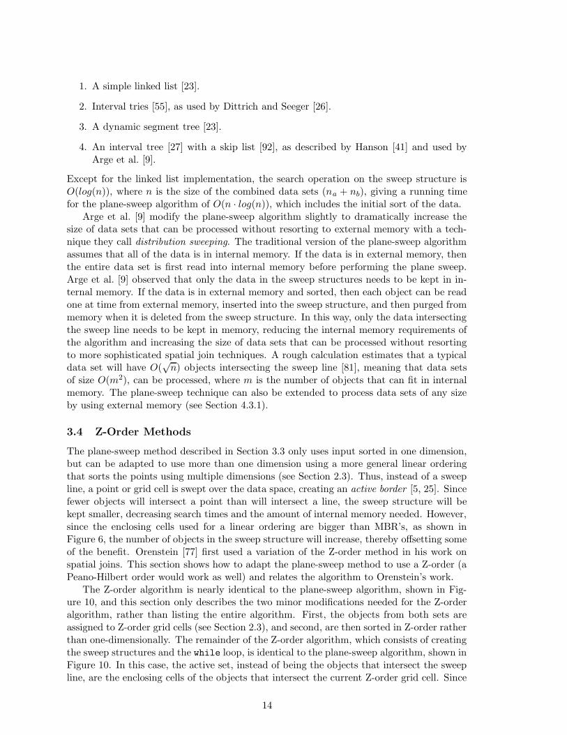
a grid cell will intersect fewer objects, the active set will be smaller and the sweep structurecan be simpler, such as a linked list [23]. Also, the sweep structure can be modified totake advantage of the regular decomposition of the Z-order cells. All of the objects in theactive set (sweep structure), which are the enclosing Z-order grid cells, will have either acontainment relation to each other or be identical. In early work on spatial joins, Orenstein[80] used a stack he called a nest to implement the sweep structure. Because the input issorted in Z-order, large objects will be inserted into the sweep structure before the smallerobjects that are enclosed by the object. These small objects will be removed before theirenclosing objects are removed. This LIFO property makes a stack the natural choice forthe sweep structure. The INSERT and REMOVE INACTIVE methods will be simple becausethey either push elements on to the stack or pop elements from the stack, respectively. TheSEARCH method is also simple since all objects in the stack will intersect the input object.If the enclosing cells intersect, the MBR’s can also be checked for intersection to furtherfilter false hits from the candidate set, assuming the MBR’s are available.

A

B

a2

a1

a3

a4

b1

Figure 11: Objects are shown from set A and set B in the order in which they appear inthe Z-order. Since the stack for the B data set will be empty until b1 is inserted, a2 anda4 do not need to be inserted into A’s stack.

Aref and Samet [6] further improved the use of the sweep structure by avoiding someinsertions. They point out that if one stack is empty, e.g., sweepStructureA, then there is noneed to insert elements into the other stack, sweepStructureB. For example, in Figure 11, ifdata set A contains the objects a1, a2, a3 and a4, then objects a2 and a4 will not intersectany objects in data set B, which contains only b1. The objects a2 and a4 need not beinserted into the stack. If one stack, sweepStructureB, is empty, then the algorithm canlook ahead to the next element, say bTop, that will be inserted into the empty stack using thesweepStructureB.FIRST function, and avoid inserting any elements into sweepStructureA

that do not intersect bTop. In Figure 11, the B stack will be empty until b1 is encountered,which becomes bTop. Therefore, a2 and a4 do not need to be added to the stack for dataset A. In a further extension, Aref and Samet [7] modify the Z-order sweep to report largerpairs first, at each stopping point (iteration of the while loop), by reporting from thebottom of the stack up, rather than from the top. Thus, the output is already in Z-order,which can be useful in a cascaded join situation.

One drawback of the Z-order sweep method is that the stacks can be filled with objectthat have large enclosing cells, even when the objects are small. For instance, as was shownin Figure 7, any object that overlaps the center point of the space will be contained in

15

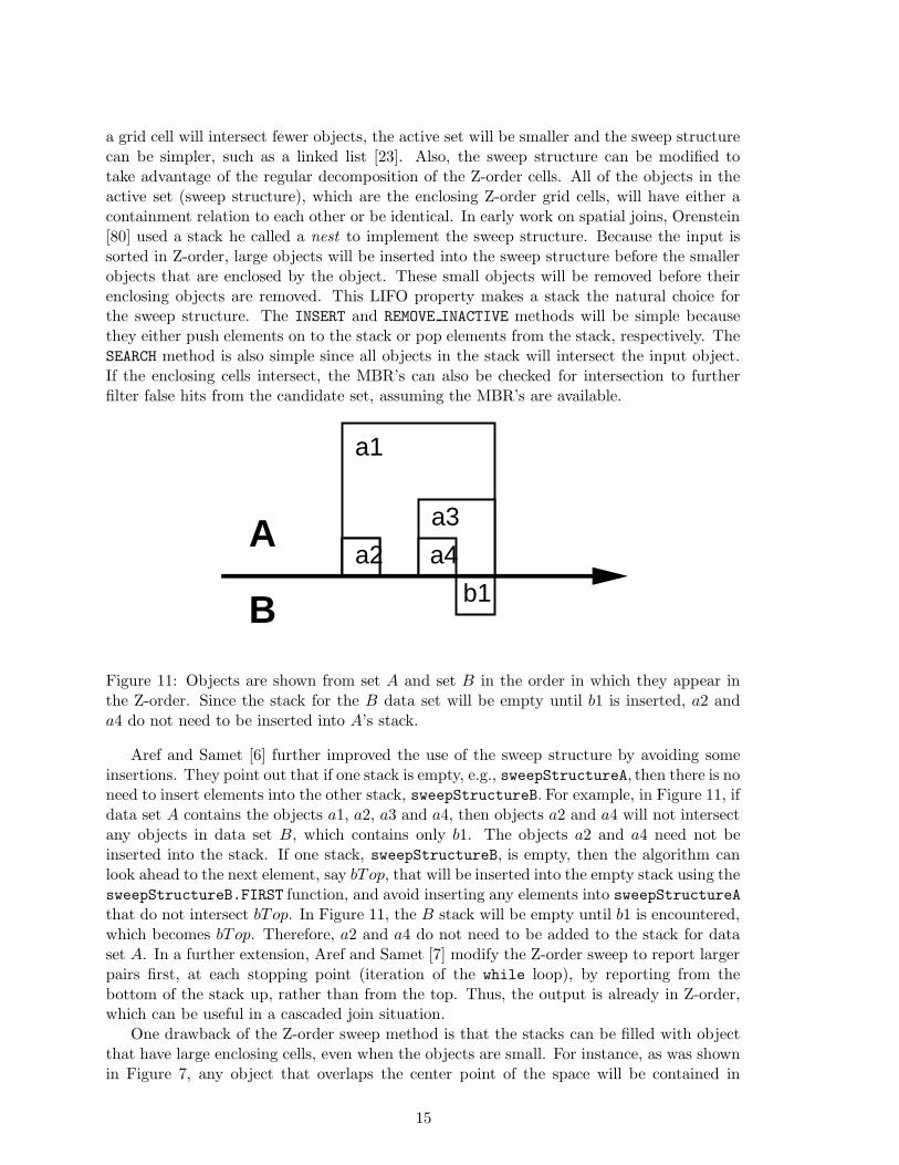
Figure 12: An object can be decomposed into multiple cells.

the highest level enclosing cell, which encloses the entire space. Such an object will beone of the first objects to enter a stack and will remain in the stack until the algorithmis through processing. This increased stack size will impair performance. To alleviate thisproblem, Orenstein [78] suggested decomposing objects into multiple cells, as shown inFigure 12. This decomposition not only reduces the size of the stack, but creates a moreaccurate approximation of the object, which reduces the number of false hits. However,these benefits are offset by the increased number of objects introduced by the redundancyand the need to remove duplicate results (recall Section 2.2). Even so, Orenstein [78] foundthat performance rapidly improves with a modest amount of decomposition. In a furtherstudy, Gaede [33] developed a formula for determining the optimal amount of redundancy.

4 The Filtering Stage – External Memory

The internal memory techniques described in Section 3 require sufficient levels of internalmemory in order to operate efficiently. For instance, to perform the nested-loop join (Sec-tion 3.1), both data sets need to be in internal memory in order to avoid repeatedly readingthe same objects in and out of external memory. To efficiently process data sets of anysize, an algorithm must use external memory to store subsets of the data (or references tothe data) during processing or the data must be indexed. This section describes filteringmethods that use external memory to efficiently process data sets of any size.

If the data is already indexed, then it is generally advantageous to use the index forthe filtering stage of a spatial join. Section 4.1 describes techniques for filtering whenboth data sets are indexed. Even if there is sufficient internal memory to use the internalmemory techniques from Section 3, if both sets are indexed, then it can be faster to usethe two-index filtering techniques 4. Section 4.2 addresses the case where only one of thedata sets is indexed. Of course, the unindexed data set can be indexed and the two-indextechniques from Section 4.1 can be used. Another approach, if only one data set is indexed,is to consider the index as a source of sorted or partitioned data and use the techniques forperforming a spatial join when neither set is indexed, which are described in Section 4.3. Ifneither data set is indexed, then it might not be efficient to build indices in order to do a

4When an external memory filtering technique should be used instead of an internal memory algorithmis an open question.

16

spatial join, especially if the indices will not be used again and immediately discarded, asis the case if the spatial join is an intermediate step in solving a complex query.

Even though the internal memory techniques in Section 3 can not be used directly, atsome point during processing, two subsets of the data that do fit in internal memory arejoined. These subsets can be two pages from indices, as in Section 4.1.1, or subsets createdby partitioning the data, as in Section 4.3. In these cases, when the internal memorytechniques from Section 3 become applicable, the reader is referred to that section, ratherthan elaborating on the in-memory join aspects of the particular algorithm.

4.1 Both Sets Indexed

If both data sets are indexed, but with incompatible types of indices, Corral et al. [24]suggest ignoring one index and performing an index-nested loop join, as described in Sec-tion 3.2. If both data sets are indexed using the same type of index, then the techniquefor performing the filtering stage of the spatial join depends on the structure of the index.Since many spatial indices are hierarchical, a spatial join algorithm for these indices alsohas a hierarchical nature. These methods are described in Section 4.1.1. Early work onspatial joins used a more general non-hierarchical approach, which are described in Sec-tion 4.1.2. Section 4.1.3 discusses a method that works with indices that transform objectsinto higher-dimensional points. Since most methods in this section join data pages or indexnodes, this issue is discussed separately, in Section 4.1.4.

4.1.1 Hierarchical Traversal

A common type of spatial index is one that can be described as a hierarchical containmentindex or a generalization tree [36], such as an R-tree [40] or a multi-level grid file [104]. Thistype of index is a tree structure in which every node of the tree corresponds to a region ofthe data space. An internal node’s region covers the regions of its sub-nodes and each nodemight or might not overlap other nodes, depending on the index type. Each node is typicallystored on one page of external memory. This section assumes that the data objects are onlystored in the leaves of the tree, though the techniques can be adapted to handle data inthe internal nodes. If both data sets are indexed using generalization trees, then a spatialjoin can be performed efficiently with a synchronized traversal of the indices. This sectiondescribes a generic synchronized traversal algorithm and then describes three variationsthat differ in how the indices are traversed, attributable to Gunther [36], Brinkhoff et al.[20], Kim et al. [53], and Huang et al. [48] 5.

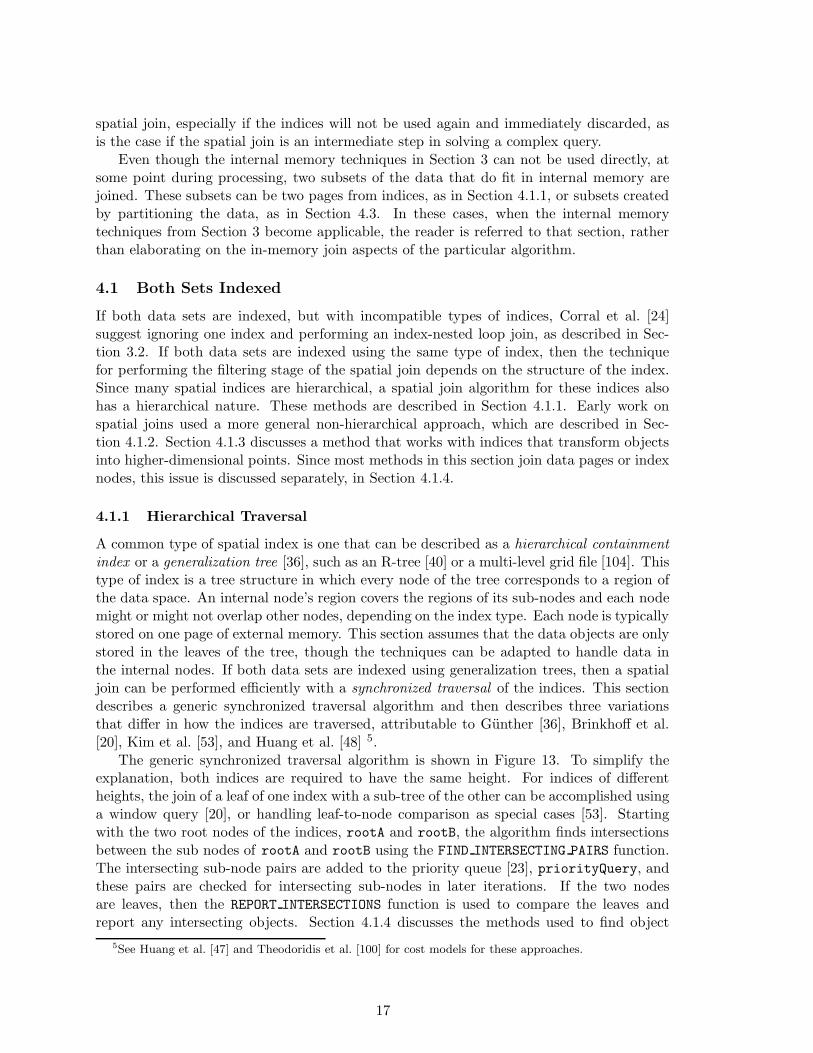
The generic synchronized traversal algorithm is shown in Figure 13. To simplify theexplanation, both indices are required to have the same height. For indices of differentheights, the join of a leaf of one index with a sub-tree of the other can be accomplished usinga window query [20], or handling leaf-to-node comparison as special cases [53]. Startingwith the two root nodes of the indices, rootA and rootB, the algorithm finds intersectionsbetween the sub nodes of rootA and rootB using the FIND INTERSECTING PAIRS function.The intersecting sub-node pairs are added to the priority queue [23], priorityQuery, andthese pairs are checked for intersecting sub-nodes in later iterations. If the two nodesare leaves, then the REPORT INTERSECTIONS function is used to compare the leaves andreport any intersecting objects. Section 4.1.4 discusses the methods used to find object

5See Huang et al. [47] and Theodoridis et al. [100] for cost models for these approaches.

17

procedure INDEX_TRAVERSAL_SPATIAL_JOIN(rootA, rootB);

begin

priorityQuery←CREATE_PRIORITY_QUEUE();

priorityQuery.ADD_PAIR(rootA, rootB);

while NOT priorityQuery.EMPTY() do

nodePair←priorityQuery.POP();

rectanglePairs←FIND_INTERSECTING_PAIRS(nodePair);

for each p ∈ rectanglePairs

if p is a pair of leaves then

REPORT_INTERSECTIONS(p);

else

priorityQuery.ADD_PAIR(p);

end if;

next p;

end loop;

end;

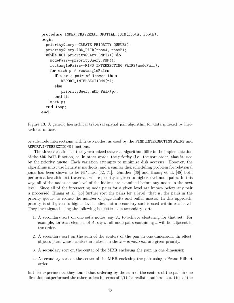
Figure 13: A generic hierarchical traversal spatial join algorithm for data indexed by hier-archical indices.

or sub-node intersections within two nodes, as used by the FIND INTERSECTING PAIRS andREPORT INTERSECTIONS functions.

The three variations of the synchronized traversal algorithm differ in the implementationof the ADD PAIR function, or, in other words, the priority (i.e., the sort order) that is usedby the priority queue. Each variation attempts to minimize disk accesses. However, thealgorithms must use heuristic methods, and a similar disk scheduling problem for relationaljoins has been shown to be NP-hard [32, 71]. Gunther [36] and Huang et al. [48] bothperform a breadth-first traversal, where priority is given to higher-level node pairs. In thisway, all of the nodes at one level of the indices are examined before any nodes in the nextlevel. Since all of the intersecting node pairs for a given level are known before any pairis processed, Huang et al. [48] further sort the pairs for a level, that is, the pairs in thepriority queue, to reduce the number of page faults and buffer misses. In this approach,priority is still given to higher level nodes, but a secondary sort is used within each level.They investigated using the following heuristics as a secondary sort:

1. A secondary sort on one set’s nodes, say A, to achieve clustering for that set. Forexample, for each element of A, say a, all node pairs containing a will be adjacent inthe order.

2. A secondary sort on the sum of the centers of the pair in one dimension. In effect,objects pairs whose centers are closer in the x− dimension are given priority.

3. A secondary sort on the center of the MBR enclosing the pair, in one dimension.

4. A secondary sort on the center of the MBR enclosing the pair using a Peano-Hilbertorder.

In their experiments, they found that ordering by the sum of the centers of the pair in onedirection outperformed the other orders in terms of I/O for realistic buffers sizes. One of the

18

drawbacks of the breadth-first approach is that, as the algorithm progresses, the priorityqueue can grow extremely large and portions of it might need to be kept in external memory.

Brinkhoff et al. [20] and Kim et al. [53] use a depth-first approach in which all of thesub-node pairs for a given node pair, p, are processed before proceeding to the next nodepair at the same level. In this case, priority is given to lower-level node pairs. As withthe breadth-first approach, heuristics can be used to reduce I/O by secondarily ordering p ′s

intersecting sub-node pairs. Brinkhoff et al. experimented with several ordering heuristicsthat secondarily sort the intersecting region of the node pairs 6:

1. In one-dimension.

2. By maximal degree, determining which node, say a, is contained in the most node-pairs, and processing a’s node pairs first.

3. In Z-order.

They found that the Z-order approach worked best for smaller buffer sizes and that the max-imal degree method worked best for larger buffer sizes. To improve performance, Brinkhoffet al. [20] use two path buffers, which keep in memory all of the ancestor nodes of thecurrent node pair. They also advocate the use of an LRU buffer to improve performance.Additionally, Brinkhoff and Kriegel [17] suggest that the performance of the spatial joincould be improved by organizing the nodes of the index into clusters which are physicallyclose on disk. During join processing, a cluster would be read into memory as a whole.However, Gunther [36] show that such clustering does not make a difference.

4.1.2 Non-Hierarchical Methods

A more general approach to performing a spatial join on indexed data is to treat the indicesas simply a partitioned data set, where the data pages of the indices are the partitions. Inthis approach, the data pages are read in an order that is meant to minimize I/O, which isa generalization of the I/O minimization heuristic orders described in Section 4.1.1. Eachpair of intersecting data pages is then read into memory and joined (see Section 4.1.4 fora discussion of joining data pages). This method is applicable to any index type with datapages. Kitsuregawa et al. [54] applied it with k-d trees [15], while Harada et al. [42] appliedit with grid files [75].

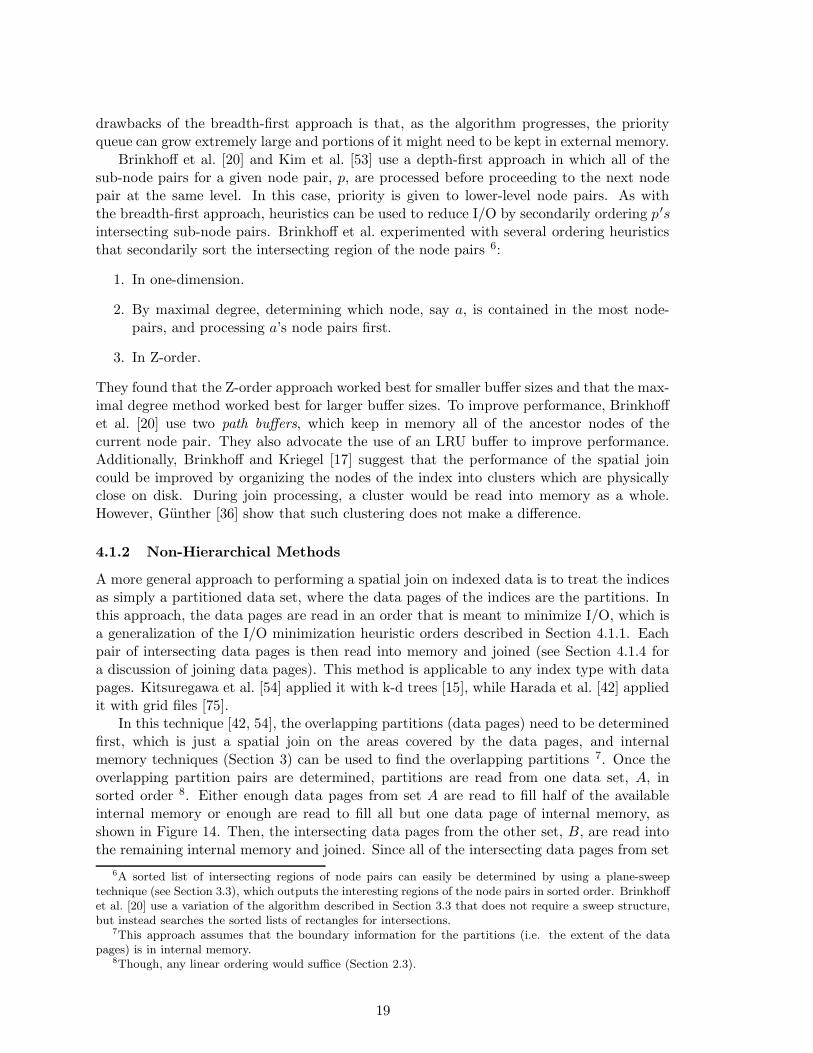
In this technique [42, 54], the overlapping partitions (data pages) need to be determinedfirst, which is just a spatial join on the areas covered by the data pages, and internalmemory techniques (Section 3) can be used to find the overlapping partitions 7. Once theoverlapping partition pairs are determined, partitions are read from one data set, A, insorted order 8. Either enough data pages from set A are read to fill half of the availableinternal memory or enough are read to fill all but one data page of internal memory, asshown in Figure 14. Then, the intersecting data pages from the other set, B, are read intothe remaining internal memory and joined. Since all of the intersecting data pages from set

6A sorted list of intersecting regions of node pairs can easily be determined by using a plane-sweeptechnique (see Section 3.3), which outputs the interesting regions of the node pairs in sorted order. Brinkhoffet al. [20] use a variation of the algorithm described in Section 3.3 that does not require a sweep structure,but instead searches the sorted lists of rectangles for intersections.

7This approach assumes that the boundary information for the partitions (i.e. the extent of the datapages) is in internal memory.

8Though, any linear ordering would suffice (Section 2.3).

19

(a) (b)

Set A

Set B

Figure 14: When joining data sets A and B, internal memory, represented as data pagesin the grid, can be (a) half filled by each of data sets A and B or (b) filled almost entirelywith data set A, leaving only one data page for data set B.

B might not fit in memory, the data pages from set B are purged from memory once theyare joined and more pages from set B are read into memory, until all of the intersectingdata pages from set B have been read. To enhance performance, Lu et al. [63] proposeprecomputing overlapping index nodes if the index will receive few updates, much like aspatial join index [93].

Corral et al. [24] apply a similar strategy for performing a spatial join between an R-tree[40] (hierarchical and non-disjoint) and a quad-tree [31] (hierarchical and disjoint) index.They propose filling internal memory efficiently by reading data pages in groups as shownin Figure 14. Additionally, they propose ordering the first set of data pages using a linearordering (see Section 2.3). Even though the two indices are of different types, the methodworks because the data pages of the indices are treated as partitions.

The methods described in this section use heuristics to determine the order of readingpartitions. In a relevant analysis, Neyer and Widmayer [74] showed that determining theoptimal read schedule to minimize the number of disk reads is NP-hard if no restrictionsare placed on the partitions. However, if the partitions do not share boundaries (that is,they do not have any sides in common), they show that the problem is easy to solve. IfG is a graph where the vertices represent the MBRs of the index nodes and an edge isplaced between all of the intersecting nodes between the two data sets, then the optimalread schedule is the Hamiltonian path through G, which can be found using an algorithmby Chiba and Nishizeki [22].

4.1.3 Transform to Multi-Dimensional Points

Unlike points, rectangles have extent, which complicates spatial join algorithms. For in-stance, since an object will not fit neatly into a partition, either the object must be replicatedinto multiple partitions or the partitions must overlap, as in an R-tree [40]. Transformationmethods avoid this problem by transforming objects into multi-dimensional points, such asused by the grid file index [75]. For example, a two-dimensional rectangle can be trans-formed into a point in four-dimensional space by using the coordinate values of the centerpoint, half of the width, and half of the height as the four values representing the rectangle.Alternatively, the rectangle can be transformed using the coordinate values of the opposingcorner points of the rectangle as the four values, which is a technique known as the corner

20

transformation.

10 12 14 16

b a

(a)

10 12 14 16

b a

10

12

14

16

Region of lines intersecting line a.

Left End Point

Right End Point

(b)

Figure 15: As an example of the transformation to multi-dimensional points, (a) two one-dimensional intervals, a and b, that overlap (b) will be near each other when mapped totwo-dimensional points. Any interval that overlaps interval a will be contained within thedotted lines when represented as a point. Furthermore, since the left point is on the x-axis,all points will be above the dashed, diagonal line.

Song et al. [96] propose a spatial join for data that is indexed using the corner trans-formation method. The indices create partitionings of the multi-dimensional points, andthe method for joining the partitions is similar to the non-hierarchical spatial join meth-ods (Section 4.1.2), which order the processing of overlapping partition pairs between thetwo data sets. However, in transformed space, calculating the overlapping partitions is notstraight-forward. For instance, when joining two indexed data sets, R and S, a region (datapage) containing points from a set R needs to be compared against a larger region contain-ing points from set S. To see why this is so, consider the one-dimensional intervals, a and b,shown in Figure 15a. In two-dimensional space, any interval that overlaps a, such as b, willbe contained within the region shown in Figure 15b, between the dashed and dotted lines.Note that all data points in transformed space are above the diagonal since the left endpoint is on the x axis. Similarly, for two-dimensional objects, such as a rectangle r (e.g. theMBR of an index node), all rectangles overlapping r will occupy a space in four dimensionssimilar to the region shown in Figure 15b (see Song et al. [96] for the exact calculation ofthis region in four dimensions). Once the overlapping partition pairs have been determined,the methods in Section 4.1.2 can be used to order reading the data pages from memory.

4.1.4 Node to Node Comparison

When joining two regions A and B, which could represent two index nodes, two data pages,or two partitions, if both regions cover the same space and fit in internal memory, thenevery object in region A needs to be joined with every other object in region B. This, ofcourse, is an internal memory spatial join and an appropriate internal memory techniquefrom Section 3 should be used. For smaller page sizes, a nested-loop join (Section 3.1)might be best because of the low overhead. For larger page sizes, the plane-sweep method(Section 3.3), as suggested by Brinkhoff et al. [20], or a Z-order sweep (Section 3.4) wouldbe more appropriate.

21

�������������������������

����������������

��������������������x

xx

x

Space A

Space B

Space A

Space B ���

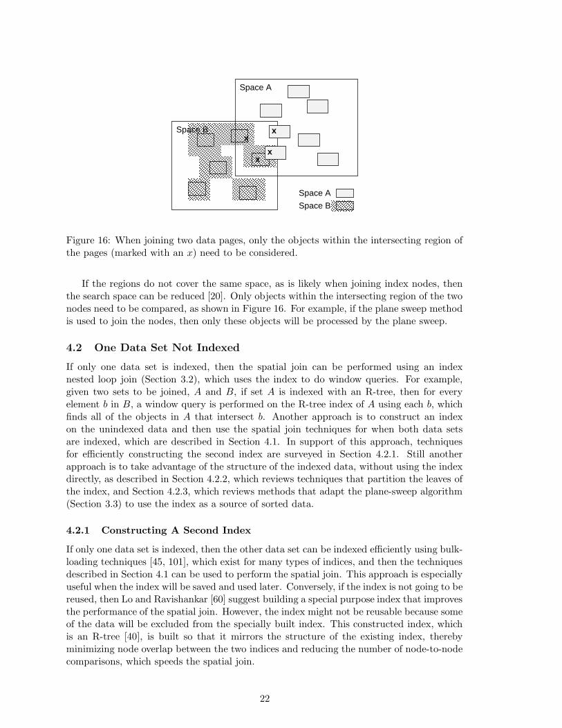
Figure 16: When joining two data pages, only the objects within the intersecting region ofthe pages (marked with an x) need to be considered.

If the regions do not cover the same space, as is likely when joining index nodes, thenthe search space can be reduced [20]. Only objects within the intersecting region of the twonodes need to be compared, as shown in Figure 16. For example, if the plane sweep methodis used to join the nodes, then only these objects will be processed by the plane sweep.

4.2 One Data Set Not Indexed

If only one data set is indexed, then the spatial join can be performed using an indexnested loop join (Section 3.2), which uses the index to do window queries. For example,given two sets to be joined, A and B, if set A is indexed with an R-tree, then for everyelement b in B, a window query is performed on the R-tree index of A using each b, whichfinds all of the objects in A that intersect b. Another approach is to construct an indexon the unindexed data and then use the spatial join techniques for when both data setsare indexed, which are described in Section 4.1. In support of this approach, techniquesfor efficiently constructing the second index are surveyed in Section 4.2.1. Still anotherapproach is to take advantage of the structure of the indexed data, without using the indexdirectly, as described in Section 4.2.2, which reviews techniques that partition the leaves ofthe index, and Section 4.2.3, which reviews methods that adapt the plane-sweep algorithm(Section 3.3) to use the index as a source of sorted data.

4.2.1 Constructing A Second Index

If only one data set is indexed, then the other data set can be indexed efficiently using bulk-loading techniques [45, 101], which exist for many types of indices, and then the techniquesdescribed in Section 4.1 can be used to perform the spatial join. This approach is especiallyuseful when the index will be saved and used later. Conversely, if the index is not going to bereused, then Lo and Ravishankar [60] suggest building a special purpose index that improvesthe performance of the spatial join. However, the index might not be reusable because someof the data will be excluded from the specially built index. This constructed index, whichis an R-tree [40], is built so that it mirrors the structure of the existing index, therebyminimizing node overlap between the two indices and reducing the number of node-to-nodecomparisons, which speeds the spatial join.

22

D

E

F

G

B

C

A

(a)

A

B C

D E F G

Seed Level

(b)

D

E

F

G

B

C

A

p

(c)

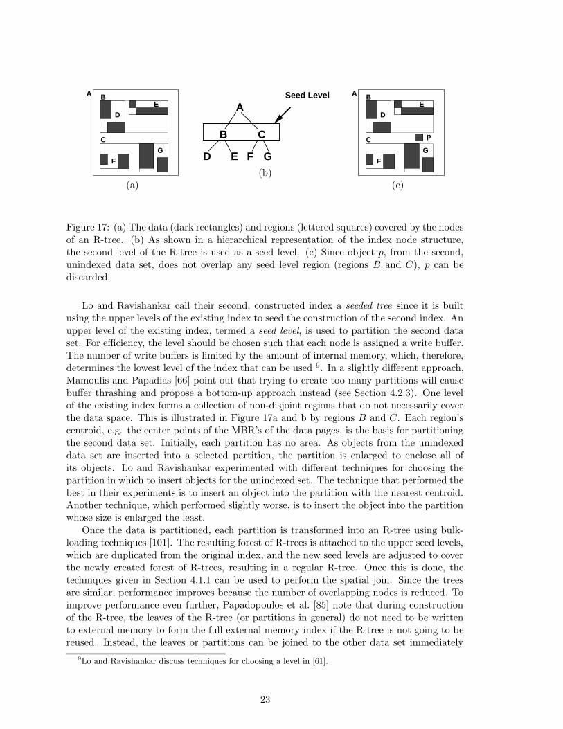
Figure 17: (a) The data (dark rectangles) and regions (lettered squares) covered by the nodesof an R-tree. (b) As shown in a hierarchical representation of the index node structure,the second level of the R-tree is used as a seed level. (c) Since object p, from the second,unindexed data set, does not overlap any seed level region (regions B and C), p can bediscarded.

Lo and Ravishankar call their second, constructed index a seeded tree since it is builtusing the upper levels of the existing index to seed the construction of the second index. Anupper level of the existing index, termed a seed level, is used to partition the second dataset. For efficiency, the level should be chosen such that each node is assigned a write buffer.The number of write buffers is limited by the amount of internal memory, which, therefore,determines the lowest level of the index that can be used 9. In a slightly different approach,Mamoulis and Papadias [66] point out that trying to create too many partitions will causebuffer thrashing and propose a bottom-up approach instead (see Section 4.2.3). One levelof the existing index forms a collection of non-disjoint regions that do not necessarily coverthe data space. This is illustrated in Figure 17a and b by regions B and C. Each region’scentroid, e.g. the center points of the MBR’s of the data pages, is the basis for partitioningthe second data set. Initially, each partition has no area. As objects from the unindexeddata set are inserted into a selected partition, the partition is enlarged to enclose all ofits objects. Lo and Ravishankar experimented with different techniques for choosing thepartition in which to insert objects for the unindexed set. The technique that performed thebest in their experiments is to insert an object into the partition with the nearest centroid.Another technique, which performed slightly worse, is to insert the object into the partitionwhose size is enlarged the least.

Once the data is partitioned, each partition is transformed into an R-tree using bulk-loading techniques [101]. The resulting forest of R-trees is attached to the upper seed levels,which are duplicated from the original index, and the new seed levels are adjusted to coverthe newly created forest of R-trees, resulting in a regular R-tree. Once this is done, thetechniques given in Section 4.1.1 can be used to perform the spatial join. Since the treesare similar, performance improves because the number of overlapping nodes is reduced. Toimprove performance even further, Papadopoulos et al. [85] note that during constructionof the R-tree, the leaves of the R-tree (or partitions in general) do not need to be writtento external memory to form the full external memory index if the R-tree is not going to bereused. Instead, the leaves or partitions can be joined to the other data set immediately

9Lo and Ravishankar discuss techniques for choosing a level in [61].

23

and then thrown out, saving I/O cost and speeding the spatial join.Lo and Ravishankar also propose extensions to filter the second data set, reducing the

size of the second data set and, thus, further speeding the join. Given two data sets A

and B, where A is indexed and B is not, they note that any object in B, say b, that doesnot intersect with the regions covered by the upper level nodes of the existing index onset A, could not intersect any object in A. Therefore, b does not need to be inserted intothe constructed index for set B. This makes the join faster, but renders the second indexunusable since it does not contain the entire data set. For example, if the constructed R-treeis not going to be reused, then objects from the second data set that do not intersect theregions covered by the seed levels do not need to be inserted into the partitions becausethey will not intersect any object in the indexed data set, as shown in Figure 17c for objectp.

4.2.2 An Index as Partitioned Data

Even if just one data set is indexed, the best approach to performing a spatial join mightnot be to construct a second index and use the synchronized traversal methods from Sec-tion 4.1.1. Instead, the index can be viewed as an existing partition of the data set andmethods similar to the non-hierarchical methods (Section 4.1.2) can be used to perform thespatial join. To create partitions from an index, the data pages are grouped to form thepartitions. The data pages can be grouped either in a top-down manner for hierarchicalindices [102] or in a bottom-up fashion for any index type [69].

In the top-down method to partitioning, proposed by van den Bercken et al. [102], theunindexed data set is partitioned based on one of the levels of the existing hierarchicalindex, e.g., the sub-nodes of the root of the indexed set, which is similar to the situationshown in Figure 17b. The partition boundaries are the MBR’s of the internal index nodesfor the chosen level, for example, regions B and C in Figure 17. The unindexed data ispartitioned based on these regions, placing each object into each partition that it overlaps,which replicates the data, requiring that duplicate removal techniques be used on the resultpairs (see Section 4.3.5).

Once the partitioning is done, each partition is joined with the objects in the sub-tree ofthe corresponding index node using any appropriate internal memory method (Section 3).If the data pages and partitions for a sub-node do not fit in memory, then the method canbe recursively applied by descending to the next level of the index. This approach worksbest if the depth of the tree is small or, conversely, if the index has a large fan out. For thisreason, van den Bercken et al. [102] propose this approach as a technique for joining twounindexed data sets, in which case an index is created with the largest possible fan out onone data set before the method is applied.

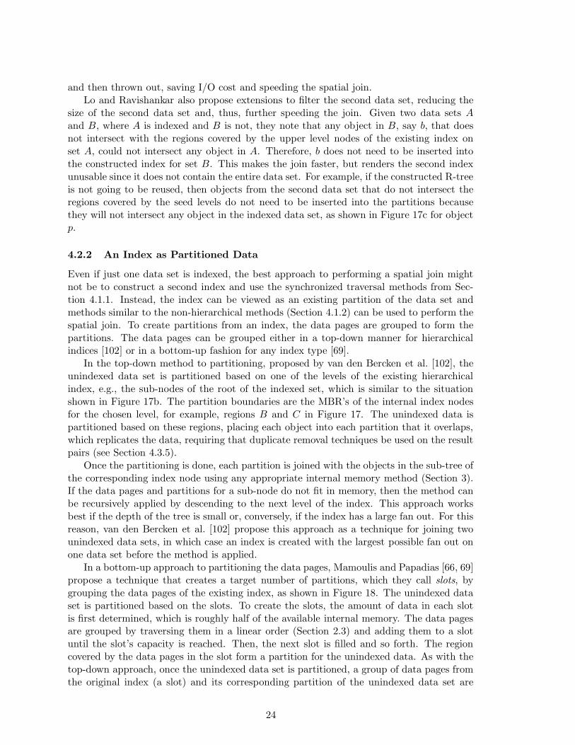
In a bottom-up approach to partitioning the data pages, Mamoulis and Papadias [66, 69]propose a technique that creates a target number of partitions, which they call slots, bygrouping the data pages of the existing index, as shown in Figure 18. The unindexed dataset is partitioned based on the slots. To create the slots, the amount of data in each slotis first determined, which is roughly half of the available internal memory. The data pagesare grouped by traversing them in a linear order (Section 2.3) and adding them to a slotuntil the slot’s capacity is reached. Then, the next slot is filled and so forth. The regioncovered by the data pages in the slot form a partition for the unindexed data. As with thetop-down approach, once the unindexed data set is partitioned, a group of data pages fromthe original index (a slot) and its corresponding partition of the unindexed data set are

24

(a) (b)

Figure 18: (a) A set of index data pages (b) are grouped to form slots, shown by thick-linedrectangles.

read into memory and joined. Due to skew, however, a slot and its partition might not fitin internal memory. In this case, the partitioning method is applied recursively until eachslot and its partition fit in memory.

4.2.3 An Index as Sorted Data

An index can also be viewed as a sorted data set, since extracting the data from an index insorted order is inexpensive using an in-order traversal of the index. In this case, the plane-sweep method (Section 3.3) can used to perform the spatial join. Generally, the plane-sweepmethod is performed after sorting both data sets. Since extracting data from an index insorted order (sorted in one-dimension) is fast, the plane-sweep technique is less expensiveto use because only one data set needs to be sorted [8].

Another approach, one that modifies the plane-sweep method, proposed by Gurret andRigaux [38], is to read the data pages from an index (they use an R-tree) in a one-dimensionalsorted order and insert entire data pages into the sweep structure. In this case, one sweepstructure will contain objects, as is normal, while the other sweep structure will containdata pages. This technique only requires a modification of the plane-sweep SEARCH routine(see Figure 10) to search for intersections between an object and a data page. Since theREMOVE INACTIVE and INSERT routines work with MBR’s and the enclosing rectangle of adata page is an MBR, these two methods do not need to be modified. Additionally, theinitial sort step of the plane-sweep algorithm needs to extract the data pages of the indexas well as sorting the unindexed data set.

If memory overflows (that is, the active set is too large to fit in internal memory),then Gurret and Rigaux [38] propose using a method in which some of the data pages ofthe index are removed (or flushed) from the sweep structure and written to disk for laterprocessing. To do this, before the plane-sweep phase of the algorithm starts, each datapage is assigned to a strip, as shown in Figure 19. The strips are created in a method thatis similar to forming slots in Section 4.2.2, except a one-dimensional sort is used. Onlyentire strips of data pages are flushed at a time. After a strip is flushed, the plane-sweepalgorithm continues. Any rectangle from the unindexed data set that overlaps the flushedstrip is also written to external memory. After the plane-sweep algorithm finishes, it is run

25

Figure 19: The leaves of an R-tree are grouped into strips, which can flushed to externalmemory if internal memory overflows.

again on the flushed data pages and rectangles written to external memory, starting fromthe point where the flush occurred. Additionally, a plane sweep on the flushed data mightalso overflow memory, in which case, the flushed data can be partitioned into strips and theentire algorithm applied recursively.

4.3 Neither Set Indexed

If neither set is indexed, then an index can be built on one or both sets of data, and thenthe techniques from Sections 4.2 and 4.1, respectively, can be used. If the index is to besaved and reused, this can make sense. If not, then other techniques that do not necessarilycreate an index might be faster 10. The key to most of these techniques lies in partitioningthe data sets so that the partitions are small enough to fit in internal memory. In otherwords, a divide-and-conquer approach is used to decompose the data sets into manageablepieces 11. Once the data is partitioned, each pair of overlapping partitions, one from eachset, is read into internal memory and internal memory techniques are used (see Section 3).This assumes that the partition pairs fit in internal memory. If they do not, then they canbe repartitioned (see Section 4.3.4) until the pairs fit.

First, before describing the partitioning methods, Section 4.3.1 discusses an extension tothe plane-sweep algorithm (Section 3.3) that can process data sets of any size by using exter-nal memory. Next, as a foundation for describing the partitioning methods in this section,Section 4.3.2 describes a generic algorithm for performing a spatial join using a partitioningtechnique. The algorithm also serves to introduce several common issues associated withthe partitioning approach – Section 4.3.3 discusses the issue of determining the numberof partitions, handling duplicate results is discussed in Section 4.3.5, and repartitioning,if any of the partition pairs do not fit in internal memory, is discussed in Section 4.3.4.The next sections then describe the more sophisticated partitioning algorithms from theliterature, grouped by how they partition the data: using grids in Section 4.3.6, using stripsin Section 4.3.7, by size in Section 4.3.8, and clustering in Section 4.3.9.

10Some techniques for unindexed data create a usable index as a by product of the spatial join, e.g. thefilter tree [56].

11Interestingly, most indices can be considered to be a partition of the data coupled with an accessstructure.

26

4.3.1 External Plane Sweep

procedure EXTERNAL_PLANE_SWEEP(setA, setB);

begin

mergedSet←SET_MERGE( setA, setB );

sortedSet←SORT_BY_LEFT_SIDE( mergedSet );

insertList←sortedSet;

sweepStructureA←CREATE_SWEEP_STRUCTURE();

sweepStructureB←CREATE_SWEEP_STRUCTURE();

while insertList 6= ∅ do

sweepStructureA.INITIALIZE();

sweepStructureB.INITIALIZE();

doOverFile←new File();

for each r in sortedSet do

if r ∈ setA then

sweepStructureB.REMOVE_INACTIVE( r );

sweepStructureB.SEARCH( r );

if r = insertList.FIRST() then

insertList.POP();

errorStatus←sweepStructureA.INSERT( r );

if errorStatus = InsufficientMemoryError then

doOverFile.WRITE( r );

end if

end if

else

sweepStructureA.REMOVE_INACTIVE( r );

sweepStructureA.SEARCH( r );

if r = insertList.FIRST() then

insertList.POP();

errorStatus←sweepStructureB.INSERT( r );

if errorStatus = InsufficientMemoryError then

doOverFile.WRITE( r );

end if

end if

end if

end for loop

insertList←doOverFile.READ_ENTIRE_FILE();

end while loop

Figure 20: An external memory version of the plane-sweep algorithm with the ability toprocess data sets of any size.

Jacox and Samet [50] extended the modified plane-sweep algorithm of Arge et al. [9](see Section 3.3) to process data sets of any size by using external memory. The algorithm,shown in Figure 20, adds an outer loop to the plane-sweep algorithm that keeps track ofwhich objects have been inserted into the sweep structure. Initially, all objects are includedin the list of objects to insert, which are stored in the insertList variable. In the first

27

run of the outer loop, the plane-sweep runs normally. If there is sufficient internal memory,the external plane-sweep performs exactly as the internal version (see Figure 10), and theouter loop does not need to run again. However, if internal memory is full, then the currentobject is not inserted into the sweep structure, but marked as not having been added tothe sweep structure. In this case, a reference to the object is saved to a file (or some otherexternal memory storage), called doOverFile. When a run of the plane-sweep finishes, thislist of objects in doOverFile serves as the list of objects to insert into the sweep structurein the next run of the outer loop, which just performs the same plane-sweep again, butdoesn’t insert the objects that were inserted on the first pass. The plane-sweep algorithmis run repeatedly until all objects have been inserted into the sweep structure. Note thaton every pass, every object is used to search the sweep structure, thereby not missing anyintersecting pairs. Also note that the algorithm merges the two sets into one data set at thebeginning of the algorithm with the SET MERGE function so that the algorithm only needsto manage one doOverFile instead of two.

4.3.2 Basic Partitioning Algorithm

1

1

2

2

3

3

4

4

Set A

Set B

Figure 21: If both data sets, A and B, are partitioned using the same grid, then each gridcell is joined with exactly one other, corresponding cell.

This section uses a simplified algorithm to illustrate a spatial join technique based onpartitioning. While the algorithm has limited practical applications, it is used as the basisfor describing more sophisticated algorithms and to describe the common issues associatedwith partitioning techniques. The basic concept is to define a grid and use it to partitionthe data from each set, sets A and B, into external memory. Each data object is placedinto each grid cell (partition) that it overlaps. Once the data is partitioned, the partitionsfor each grid cell of set A are joined with the corresponding partition of set B using one ofthe internal memory methods from Section 3. For example, in Figure 21, both sets A andB are partitioned using the same grid, and then, each corresponding cell is joined with theother. Grid cell 1 from set A, for instance, is joined with cell 1 from set B, and so forth.

In the algorithm, shown in Figure 22, the first step is to determine how many parti-tions are needed. The goal is to create partitions that are small enough, when paired witha corresponding partition, to fit in internal memory. To do this, the algorithm first cal-culates the minimum number of partitions needed, minNumberOfPartitions, as the totalstorage costs of the objects in both sets divided by the available internal memory. The

28

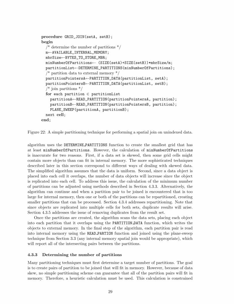
procedure GRID_JOIN(setA, setB);

begin

/* determine the number of partitions */m←AVAILABLE_INTERNAL_MEMORY;

mbrSize←BYTES_TO_STORE_MBR;

minNumberOfPartitions← (SIZE(setA)+SIZE(setB))*mbrSize/m;

partitionList←DETERMINE_PARTITIONS(minNumberOfPartitions);

/* partition data to external memory */partitionPointersA←PARTITION_DATA(partitionList, setA);

partitionPointersB←PARTITION_DATA(partitionList, setB);

/* join partitions */for each partition ∈ partitionList

partitionA←READ_PARTITION(partitionPointersA, partition);

partitionB←READ_PARTITION(partitionPointersB, partition);

PLANE_SWEEP(partitionA, partitionB);

next cell;

end;

Figure 22: A simple partitioning technique for performing a spatial join on unindexed data.

algorithm uses the DETERMINE PARTITIONS function to create the smallest grid that hasat least minNumberOfPartitions. However, the calculation of minNumberOfPartitions

is inaccurate for two reasons. First, if a data set is skewed, then some grid cells mightcontain more objects than can fit in internal memory. The more sophisticated techniquesdescribed later in this section correspond to different ways of dealing with skewed data.The simplified algorithm assumes that the data is uniform. Second, since a data object isplaced into each cell it overlaps, the number of data objects will increase since the objectis replicated into each cell. To address this issue, the calculation of the minimum numberof partitions can be adjusted using methods described in Section 4.3.3. Alternatively, thealgorithm can continue and when a partition pair to be joined is encountered that is toolarge for internal memory, then one or both of the partitions can be repartitioned, creatingsmaller partitions that can be processed. Section 4.3.4 addresses repartitioning. Note thatsince objects are replicated into multiple cells for both sets, duplicate results will arise.Section 4.3.5 addresses the issue of removing duplicates from the result set.

Once the partitions are created, the algorithm scans the data sets, placing each objectinto each partition that it overlaps using the PARTITION DATA function, which writes theobjects to external memory. In the final step of the algorithm, each partition pair is readinto internal memory using the READ PARTION function and joined using the plane-sweeptechnique from Section 3.3 (any internal memory spatial join would be appropriate), whichwill report all of the intersecting pairs between the partitions.

4.3.3 Determining the number of partitions

Many partitioning techniques must first determine a target number of partitions. The goalis to create pairs of partition to be joined that will fit in memory. However, because of dataskew, no simple partitioning scheme can guarantee that all of the partition pairs will fit inmemory. Therefore, a heuristic calculation must be used. This calculation is constrained

29

by the following factors:

1. The amount of internal memory, which determines the number of objects that can bejoined at a time using internal memory techniques.

2. The replication rate, which is the actual number of objects inserted into the partitions,which includes duplicates.

3. The amount of internal memory also limits the number of write buffers that can beused to partition the data to external memory.

Within these constraints, different techniques either try to maximize or minimize the numberof partitions. A minimum number of partitions might be calculated in order to reducereplication, which reduces the number of pairs that need to be joined. A maximum numberof partitions minimizes the chances of a costly repartitioning.

The simplest calculation, ignoring data skew and replication, derives the target numberof partitions by dividing the total storage costs of the objects by the available internalmemory. The total storage costs of the objects is the number of objects multiplied by thesize of an object in bytes, referred to as objectSize. In an implementation, objectSize

might be the sum of the size of a rectangle (MBR) in bytes and the size of an object pointeror object key. To account for replication, a scale factor can be added to the calculation.The replication rate depends on the data set and the partitioning scheme. In one set ofexperiments [88], the replication rate was found to be 3-10%. Incorporating the replicationscale factor, r, the calculation for the minimum number of initial partitions is:

r · (|setA|+ |setB|) · objectSize

m, (1)

where m is the available internal memory. However, this equation does not take into accountdata skew and is only an estimate. In the worst case, with severely skewed data, most of thedata could be in one partition. In this case, repartitioning is required (see Section 4.3.4).

Equation 1 applies to internal memory methods that require all of the data to be readinto internal memory before processing begins. Arge et al. [9] showed that the plane-sweepmethod can process more data than can fit in internal memory, see Section 3.3. However,the exact amount of data that can be processed is dependent on the data set, specificallythe maximum density of the data set [29, 50, 100], which is just the maximum number ofobjects in the active set. However, this value is difficult to calculate for a given data set.Most of the algorithms described in this section do not use this technique because it is stillrelatively new and has not been fully exploited in the literature.

The maximum number of partitions is limited by internal memory in that internal mem-ory limits the number of external memory write buffers. Typically, for better performance,when writing to external memory, a page of internal memory is filled before it is flushed toexternal memory. This places a hard limit on the maximum number of partitions.

The principal motivation for getting the right number of partitions is to avoid reparti-tioning (see Section 4.3.4). However, the more partitions there are, the greater the replica-tion. Some evidence suggests that this replication does not have a significant impact on thetotal processing time [106]. In this case, creating the maximum number of partitions mightoptimize performance. Conversely, internal memory algorithms might perform better withsmaller partitions, thereby improving overall performance. From the literature, it is unclearwhat the best choice is for the number of partitions and thus, we leave this choice as anopen question.

30

4.3.4 Repartitioning

The goal of partitioning is to create partitions that are small enough to be processed by inter-nal memory techniques (Section 3). However, the initial partitioning phase (Section 4.3.3)might create partitions that are too large because of data replication or skewed data. Ifthis occurs, then the partition pairs that are too large can be further sub-divided using theoriginal partitioning scheme, creating a finer grid. If this repartitioning fails, then the pro-cess can be repeated recursively until all of the partition pairs can be processed by internalmemory methods.

Repartitioning can occur immediately after the initial partitioning, or it might be nec-essary to do it later, after some partition pairs have been joined. With the basic internalmemory techniques, such as the nested-loop join (Section 3), the size of the data sets thatcan be processed is known, in which case, any over-full partition pairs can be repartitionedimmediately, before joining any of the partitions. However, with other internal memorytechniques, such as the plane-sweep extension [9], it might not be known whether or not apartition pair is small enough. In this case, repartitioning is done only when an internalmemory technique fails because its sweep structure has grown too large for the availableinternal memory. Any result pairs generated for the current partition pair need to bediscarded since the results will be regenerated after repartitioning.

If a partition pair to be joined, say A and B, is too large for the available internalmemory, Dittrich and Seeger [26] propose repartitioning only one of the data sets, sayA, first, and then joining each sub-partition with B. If this fails to create small enoughpartitions, then the other data set, B can be repartitioned. This process can also occurrecursively until small enough partitions are achieved.

4.3.5 Avoiding Duplicate Results

Partition Boudnary

ba

Figure 23: An intersection between objects a and b is reported from both partitions intowhich they are inserted, creating a duplicate result.

If partitioning the data results in object replication, then duplicate results will be re-ported. For instance, if a pair of overlapping objects is split by a partition boundary,then the intersecting pair will be reported when each partition is processed, as shown inFigure 23. Some experiments have shown that replication does not add considerably toprocessing [106], though other experiments have shown the opposite [64]. In either case,

31

duplicate results need to be removed from the candidate set to avoid extra processing dur-ing the refinement stage (Section 6). The duplicates can be removed with an extra stepbetween the filtering stage and the refinement stage or combined with refinement. Withsome algorithms, duplicate results can be detected during filtering and removed in-line.

One way to remove duplicate results from the candidate set after the filtering stage is tosort the candidate set and then scan the sorted list, removing duplicates. Some refinementtechniques sort the candidate set first, and thus, this duplicate removal technique can beused without a loss of performance (see Section 6). However, to sort the candidate set,the entire candidate set must be produced first. In some systems, such as a pipe-linedsystems [35], results need to be produced continuously. In this case, in-line duplicate removaltechniques are preferred.

Partition A

Partition Bx

Figure 24: The reference point method for in-line duplicate avoidance only reports anintersecting pair if a point in the intersecting region, x, is within the current partition. Thepoint must be chosen consistently, such as always the lower left corner.

To avoid reporting duplicate results during the filter stage, in-line duplicate removal,the internal memory spatial join techniques (Section 3) can be modified with a simple testwhich is applied when the rectangles are checked for intersection. The technique, termedthe reference point method [5, 26], calculates a point based within the intersecting region ofthe two objects. The pair is only reported if this point is within the current partition. Thetest point can lie anywhere within the intersecting region of the two objects, such as thecentroid of the region or a corner point, but must be chosen consistently 12. For instance,as shown in Figure 24, reference point, x, is the lower left corner point of the intersectingregion of the two rectangles. Since point x only lies within the B partition, the intersectingrectangles will only be reported when the B partition is processed, but not when the A

partition is processed, which also includes the rectangle pair.

4.3.6 Partitioning Using Grids

No technique uses a simple grid as did the generic algorithm in Figure 22, as it is onlyuseful for uniform distributions. However, Patel and Dewitt [88] use a uniform grid asa starting point. First, the data space is divided into a uniform grid, where the numberof grid cells, which they call tiles, is greater (typically much greater) than the number of

12To use the reference point method, the approximations of the objects can not be clipped, that is, the fullMBR must be stored and not just the portion of the object within a partition (most partitioning methodsdon’t use clipping).

32

Partition 1

Partition 2

Partition 3

Figure 25: Non-contiguous grid cells are grouped to form three partitions.

2,3

1, 2, 3

3

1

1

2

1,3

1,2

Figure 26: Forming partitions from non-contiguous grid cells helps to prevent data skewproblems by creating partitions of equal size. Even though the data is clustered in the lowerleft corner, the partitioning scheme used in Figure 25 results in each partition containingfour objects. Each object is labeled with the partitions in which it will be placed.

desired partitions. The grid cells are then grouped into partitions using a mapping functionin such a way as to minimize skew by, hopefully, creating partitions that contain a similarnumbers of objects. For example, in Figure 25, the grid cells are grouped to form threepartitions. Even if the data is skewed, each partition will cover part of the data set, asshown in Figure 26. Note that the data is not physically partitioned into the grid cells, butonly into the final partitions. In other words, grid cells are assigned to partitions first, andthen the data is partitioned.

Patel and Dewitt [88] do not proscribe a particular mapping, but only suggest using someform of a hashing function to assign the cells to partitions. The hash function should bechosen to distribute the data evenly between the partitions and is dependent on the data set.As an example, Patel and Dewitt use a round-robin order, that scans the grid in row-majororder and alternates assigning the cells among the partitions, as is shown in Figure 25. In theexample, because the grid cells are not contiguous, the partitions have a larger perimeter,leading to increased data replication since a larger perimeter provides more opportunities foran object to intersect the perimeter. Using more initial grid cells increases the uniformity

33

of the distribution because areas of skewed, dense data are distributed amongst severalpartitions, but using more tiles also increases the replication of objects across partitions.Experiments [88] showed that many more grid cells can create near uniform distributionsfrom skewed data sets, but the replication rate can also increase rapidly. In the experiments,Tiger data [76] had a replication rate of about 2.5% with 100 grid cells per partition whileSequoia data [97] had a replication rate of 10%.

Zhou et al. [106] use a variation of this technique in which the data is physically par-titioned into the grid cells, first. Since the grid cell sizes are known, the partitions canbe formed by grouping contiguous cells until a desired partition size, as determined usingmethods from Section 4.3.3, is reached. This approach reduces the amount of replicationbecause the partition boundary is smaller. The cells can be grouped using any linear order,such as a Z-order (Section 2.3). If any grid cells remain after the maximum number ofpartitions have been formed, then they can be assigned to the partitions with the leastobjects.

4.3.7 Partitioning With Strips

Sort/Sweep Direction

Strip 1

Strip 2

Strip 3

Strip 4

Sweep Line

Figure 27: In strip partitioning, the data is partitioned into strips and sorted parallel tothe strip to take advantage of the plane-sweep modification described in Section 3.3. Thesweep is repeated four times, once for each strip. The actual height of the sweep line is theheight of the strip.

Arge et al. [9] partition the data into strips so that they can take advantage of theirmodification to the plane-sweep algorithm (Section 3.3). For the plane-sweep method, afterthe data is sorted, it is partitioned into strips that are parallel to the sort direction, asshown in Figure 27, 13 With the modified plane-sweep method, the amount of data thatcan be processed with a given amount of internal memory is limited by the maximum size ofthe active set. When the data is partitioned into strips, the maximum size of the active setis the maximum number of objects that intersect the sweep line, which follows the heightof the strip. By appropriately limiting the height of the strip, which can be a difficultcalculation (see Section 4.3.3), the width of the strip can be of any length, even infinite, intheory. Also, because strips are used, fewer partitions are needed than in the grid methodof Section 4.3.6. Thus, if the grid method needs k partitions to process the data without

13Guting and Schilling [39] also used a form of strip partitioning to solve the rectangle intersection problemusing external memory.

34

repartitioning, then the strip method can process the same data with only√

k partitions.For instance, if the grid method creates a regular grid with sixteen cells, then the stripmethod can process the same data with four strips. In other words, the strip method wouldjust ignore the vertical lines of the grid method. Additionally, since fewer partitions areused, less data is replicated.

4.3.8 Partitioning By Size

a

(a)

b

(b)

c

(c)

Figure 28: To partition by size, objects are associated with the level where they first intersecta grid. (a) Object a is associated with the root space, the highest level, since it intersectsthe first (coarsest) grid level with four grid cells. (b) Object b is associated with the nextlevel since it intersects the next finer grid level with sixteen cells. (c) Object c is associatedwith an even lower level.

Koudas and Sevcik [56] roughly partition the data by size, using a series of finer andfiner grids, as shown in Figure 28. Each successive grid is derived by subdividing each cellinto four equal sized cells. To partition the data, each object is placed into the partitionassociated with the finest grid in which the object does not intersect the grid lines. Forexample, as shown in Figure 28a, object a crosses the coarsest partitioning, and therefore,goes into the first partition. The next partition is similarly composed of objects that donot fit in the first partition and which cross partition boundaries for sixteen equal sizedpartitions, as shown Figure 28b. Each lower level partition, such as the one containingobject c in Figure 28c, is similarly formed. In essence, each partition is a filter and objectsfall through to the lowest level partition where a partition boundary is crossed.

35

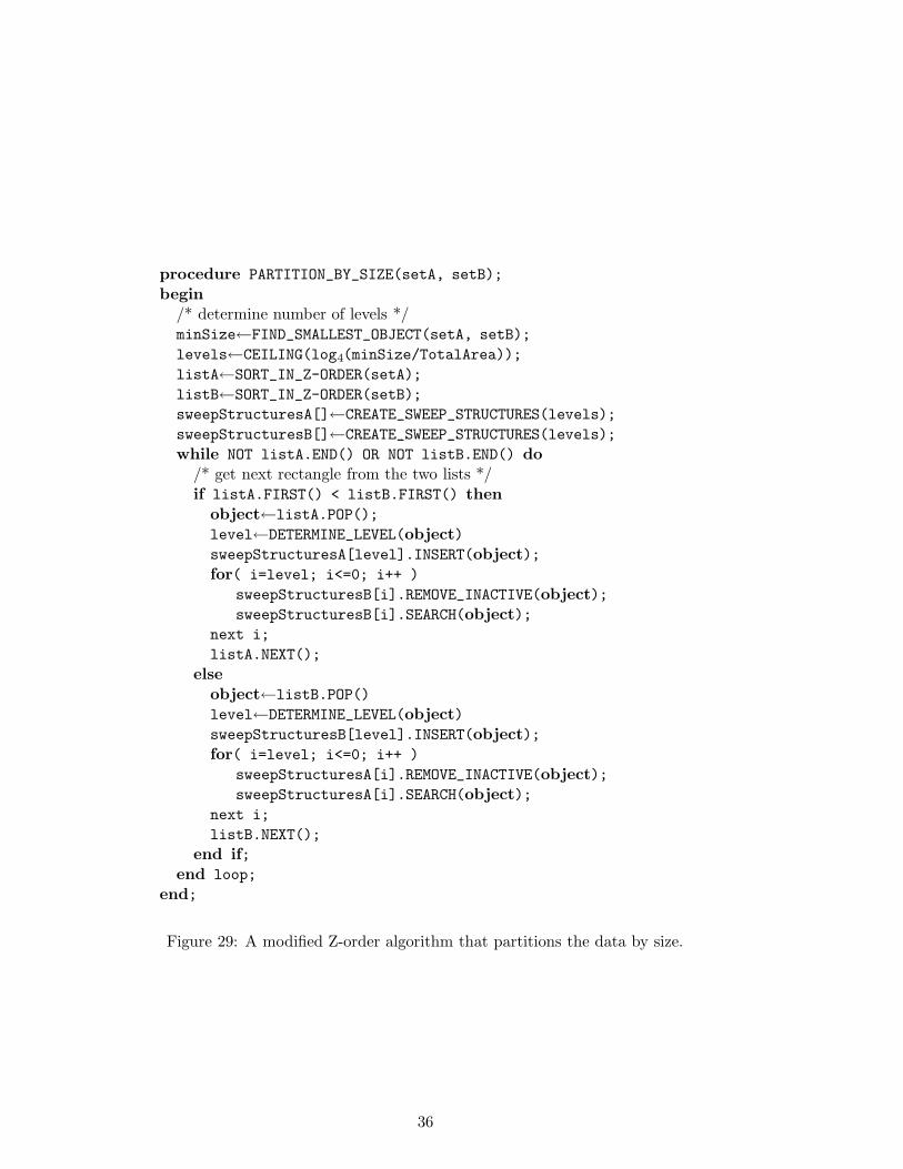
procedure PARTITION_BY_SIZE(setA, setB);

begin

/* determine number of levels */minSize←FIND_SMALLEST_OBJECT(setA, setB);

levels←CEILING(log4(minSize/TotalArea));

listA←SORT_IN_Z-ORDER(setA);

listB←SORT_IN_Z-ORDER(setB);

sweepStructuresA[]←CREATE_SWEEP_STRUCTURES(levels);

sweepStructuresB[]←CREATE_SWEEP_STRUCTURES(levels);

while NOT listA.END() OR NOT listB.END() do

/* get next rectangle from the two lists */if listA.FIRST() < listB.FIRST() then

object←listA.POP();

level←DETERMINE_LEVEL(object)

sweepStructuresA[level].INSERT(object);

for( i=level; i<=0; i++ )

sweepStructuresB[i].REMOVE_INACTIVE(object);

sweepStructuresB[i].SEARCH(object);

next i;

listA.NEXT();

else

object←listB.POP()

level←DETERMINE_LEVEL(object)

sweepStructuresB[level].INSERT(object);

for( i=level; i<=0; i++ )

sweepStructuresA[i].REMOVE_INACTIVE(object);

sweepStructuresA[i].SEARCH(object);

next i;

listB.NEXT();

end if;

end loop;

end;

Figure 29: A modified Z-order algorithm that partitions the data by size.

36

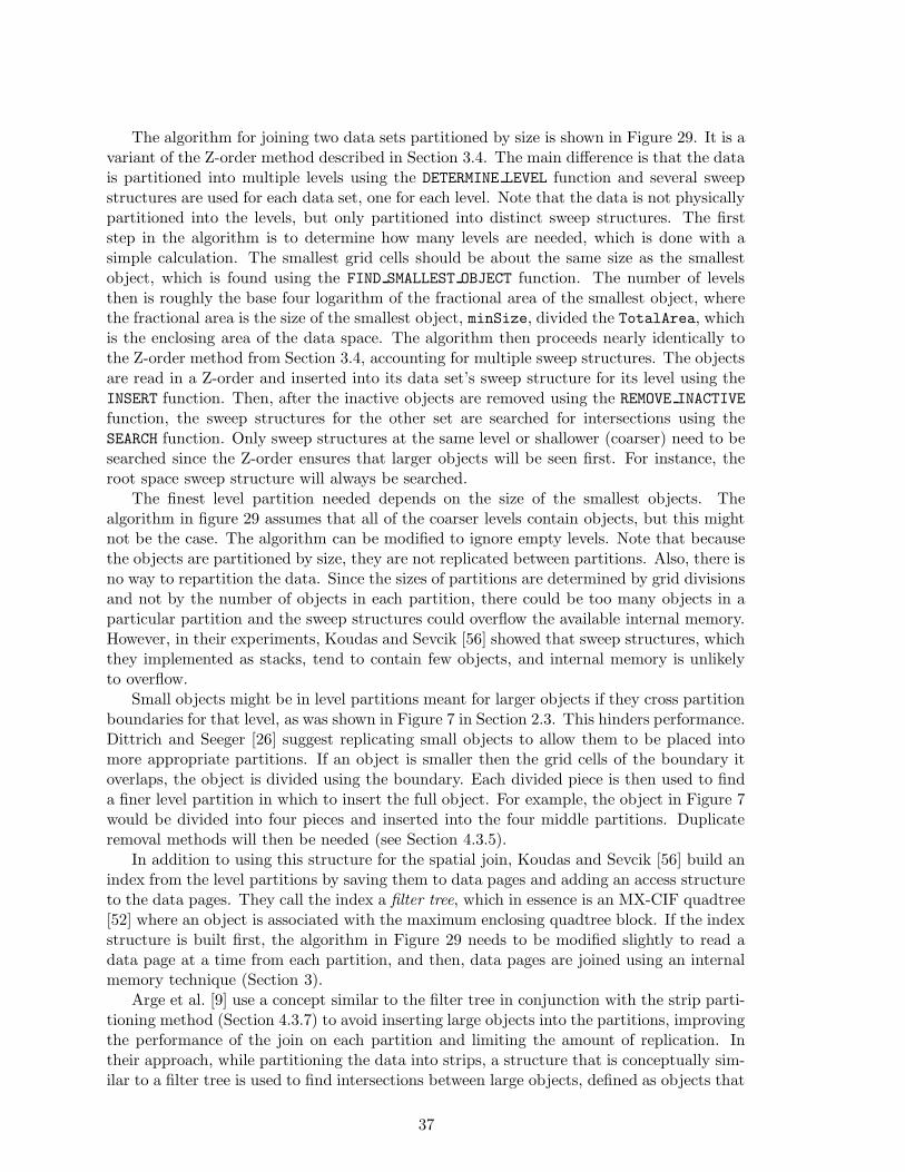
The algorithm for joining two data sets partitioned by size is shown in Figure 29. It is avariant of the Z-order method described in Section 3.4. The main difference is that the datais partitioned into multiple levels using the DETERMINE LEVEL function and several sweepstructures are used for each data set, one for each level. Note that the data is not physicallypartitioned into the levels, but only partitioned into distinct sweep structures. The firststep in the algorithm is to determine how many levels are needed, which is done with asimple calculation. The smallest grid cells should be about the same size as the smallestobject, which is found using the FIND SMALLEST OBJECT function. The number of levelsthen is roughly the base four logarithm of the fractional area of the smallest object, wherethe fractional area is the size of the smallest object, minSize, divided the TotalArea, whichis the enclosing area of the data space. The algorithm then proceeds nearly identically tothe Z-order method from Section 3.4, accounting for multiple sweep structures. The objectsare read in a Z-order and inserted into its data set’s sweep structure for its level using theINSERT function. Then, after the inactive objects are removed using the REMOVE INACTIVE

function, the sweep structures for the other set are searched for intersections using theSEARCH function. Only sweep structures at the same level or shallower (coarser) need to besearched since the Z-order ensures that larger objects will be seen first. For instance, theroot space sweep structure will always be searched.

The finest level partition needed depends on the size of the smallest objects. Thealgorithm in figure 29 assumes that all of the coarser levels contain objects, but this mightnot be the case. The algorithm can be modified to ignore empty levels. Note that becausethe objects are partitioned by size, they are not replicated between partitions. Also, there isno way to repartition the data. Since the sizes of partitions are determined by grid divisionsand not by the number of objects in each partition, there could be too many objects in aparticular partition and the sweep structures could overflow the available internal memory.However, in their experiments, Koudas and Sevcik [56] showed that sweep structures, whichthey implemented as stacks, tend to contain few objects, and internal memory is unlikelyto overflow.

Small objects might be in level partitions meant for larger objects if they cross partitionboundaries for that level, as was shown in Figure 7 in Section 2.3. This hinders performance.Dittrich and Seeger [26] suggest replicating small objects to allow them to be placed intomore appropriate partitions. If an object is smaller then the grid cells of the boundary itoverlaps, the object is divided using the boundary. Each divided piece is then used to finda finer level partition in which to insert the full object. For example, the object in Figure 7would be divided into four pieces and inserted into the four middle partitions. Duplicateremoval methods will then be needed (see Section 4.3.5).

In addition to using this structure for the spatial join, Koudas and Sevcik [56] build anindex from the level partitions by saving them to data pages and adding an access structureto the data pages. They call the index a filter tree, which in essence is an MX-CIF quadtree[52] where an object is associated with the maximum enclosing quadtree block. If the indexstructure is built first, the algorithm in Figure 29 needs to be modified slightly to read adata page at a time from each partition, and then, data pages are joined using an internalmemory technique (Section 3).

Arge et al. [9] use a concept similar to the filter tree in conjunction with the strip parti-tioning method (Section 4.3.7) to avoid inserting large objects into the partitions, improvingthe performance of the join on each partition and limiting the amount of replication. Intheir approach, while partitioning the data into strips, a structure that is conceptually sim-ilar to a filter tree is used to find intersections between large objects, defined as objects that

37

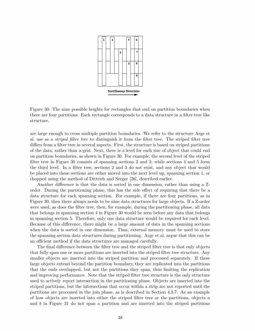
2

3

4

5

6

7

8

9

1

Sort/Sweep Direction

Figure 30: The nine possible heights for rectangles that end on partition boundaries whenthere are four partitions. Each rectangle corresponds to a data structure in a filter-tree likestructure.

are large enough to cross multiple partition boundaries. We refer to the structure Arge etal. use as a striped filter tree to distinguish it from the filter tree. The striped filter treediffers from a filter tree in several aspects. First, the structure is based on striped partitionsof the data, rather than a grid. Next, there is a level for each size of object that could endon partition boundaries, as shown in Figure 30. For example, the second level of the stripedfilter tree in Figure 30 consists of spanning sections 2 and 3, while sections 4 and 5 formthe third level. In a filter tree, sections 2 and 3 do not exist, and any object that wouldbe placed into these sections are either moved into the next level up, spanning section 1, orchopped using the method of Dittrich and Seeger [26], described earlier.

Another difference is that the data is sorted in one dimension, rather than using a Z-order. During the partitioning phase, this has the side effect of requiring that there be adata structure for each spanning section. For example, if there are four partitions, as inFigure 30, then there always needs to be nine data structures for large objects. If a Z-orderwere used, as does the filter tree, then, for example, during the partitioning phase, all datathat belongs in spanning section 4 in Figure 30 would be seen before any data that belongsin spanning section 5. Therefore, only one data structure would be required for each level.Because of this difference, there might be a large amount of data in the spanning sectionswhen the data is sorted in one dimension. Thus, external memory must be used to storethe spanning section data structures during partitioning. Arge et al. argue that this can bean efficient method if the data structures are managed carefully.

The final difference between the filter tree and the striped filter tree is that only objectsthat fully span one or more partitions are inserted into the striped filter tree structure. Anysmaller objects are inserted into the striped partition and processed separately. If theselarge objects extend beyond the partition boundary, they are replicated into the partitionsthat the ends overlapped, but not the partitions they span, thus limiting the replicationand improving performance. Note that the striped filter tree structure is the only structureused to actively report intersection in the partitioning phase. Objects are inserted into thestriped partitions, but the intersections that occur within a strip are not reported until thepartitions are processed in the join phase, as is described in Section 4.3.7. As an exampleof how objects are inserted into either the striped filter tree or the partitions, objects a

and b in Figure 31 do not span a partition and are inserted into the striped partitions

38

a

b c d

1

2

3

Figure 31: The filter tree concept can be used to avoid having to insert large objects intothe partitions when the data is partitioned into strips. Since objects c and d span partitions,they are replicated into the partitions that the ends overlap, but not the partitions that theyspan (partition 2). The spanning portions are inserted into the striped filter tree, whichimmediately checks for intersections with other large objects. Since objects a and b do notspan any partitions, they are simply inserted into the partitions they overlap and joined asdescribed in Section 4.3.7.

they overlap for later processing. On the other hand, object c spans partition 2, and it isinserted into the spanning section for partition 2 and immediately joined with any otherlarge objects using the striped filter tree. Since the ends of object c overlap partitions 1and 3, object c is inserted, with replication, into both of these striped partitions for laterprocessing. Similarly, object 4 is inserted into the spanning section for partition 2 in thefilter tree. Since the lower end of object 4 is on the partition boundary, it does not need tobe inserted into partition 3, but only into partition 1 for later processing.

4.3.9 Data-Centric Partitioning

Lo and Ravishankar [61, 62] cluster the data into partitions. One of the data sets, sayset A, is first sampled and a nearest-center heuristic is used to identify clusters of thesampled objects. The centroids of the clusters form the basis of the partitions. Initially,each partition is just the identified point, with no area. As objects from set A are insertedinto the partitions, the partition boundaries are expanded to enclose the inserted objects.Thus, a partition boundary is the enclosing MBR of the objects in the partition. Data isinserted into the partitions using a choice of heuristics, such as inserting into the partitionwhose size grows the least by area or into the partition whose centroid is closest. Note thatthis process results in non-disjoint partitions. Once set A is inserted, the resulting partitionboundaries are used to partition the second data set, say B. Objects from set B are insertedinto each partition that they overlap. Each partition for set A then needs to be joined withonly one partition from set B using any appropriate internal memory method (Section 3).Duplicate results do not occur since each object from set A is only in one partition. Onebenefit of building non-disjoint partitions is that the partitions might not cover the entiredata space. If this is the case with set A, then objects from set B that do not overlap anypartition can be discarded since they could not be joined with any rectangle in set A.

39

5 Filtering Extensions

This section discusses approximations other than MBRs that can be used for filtering anda method for making the filtering phase non-blocking. Section 5.1 surveys techniques forproducing better candidate sets with fewer false hits by using better approximations. Sec-tion 5.2 discusses tests and approximations that can be used to identify true hits, thatis, pairs of objects that definitely intersect. These pairs can be immediately reported andthen removed from the candidate set, meaning that they are not passed to the more ex-pensive refinement stage. Section 5.3 describes a technique for making the filtering phasenon-blocking.

5.1 False Hit Filtering

The MBR is not the only approximation that can be used during the filtering stage. Otherapproximations can be used if the filtering method is adapted to use the alternate approxi-mation. Additionally, other approximations can be used as a secondary filter after the initialfiltering stage to prune some false hits from the candidate set. To do this, the candidateset is scanned and an intersection test is performed on each pair of objects using a differentapproximation than was used to do the initial filtering. This second approximation shouldbe stored since calculating the approximation on the fly requires the full object to be readinto memory.

(a) (b) (c)

(d) (e)

Figure 32: Alternate approximations to MBR’s include: (a) the rotated minimum boundingrectangle, (b) the minimum bounding circle, (c) the minimum bounding ellipse, (d) theconvex hull, and (e) the minimum bounding n-corner polygon (e.g., 5-corner).

Brinkhoff et al. [18] investigated false hit filtering methods that use approximations

40

other than the MBR, which are shown in Figure 32. The approximations are:

1. The rotated minimum bounding rectangle.

2. The minimum bounding circle.

3. The minimum bounding ellipse.

4. The convex hull.

5. The minimum bounding n-corner polygon (e.g., 5-corner).

They found that using a better approximation generally reduces the number of false hits.The convex hull and 5-corner approximation performed especially well. However, the higherstorage costs, the increased complexity of calculating the approximation, and the increasedcomplexity of the intersection test can mitigate the benefit. Even so, Brinkhoff and Kriegel[16] found that additional filtering with these approximations can improve total performancesignificantly.

(a)

Covered

Mostly Covered

Partially Covered

Not Covered

(b)

Figure 33: An object (a) is approximated using a four color scheme (b) by imposing agrid over the object and coloring the cells depending on whether they are covered, mostlycovered, partially covered, or not covered.

Zimbrao and de Souza [110] propose using a 4-color raster approximation for secondaryfiltering. As shown in Figure 33, a grid is imposed over each object and grid cells are coloreddepending on whether they are covered, mostly covered, partially covered, or not covered.To check for intersections, the two raster approximations of the objects are compared, takinginto account the different offsets and scales of the grids. The number of grid cells can beadjusted to obtain more accurate results for filtering, but at the expense of higher storagecosts.

Veenhoff et al.[103] propose an approximation that is constructed by rotating two par-allel lines around the object. In other words, two more sides, parallel to each, other areadded by chopping two corners of the MBR, as shown in Figure 34, creating a better ap-proximation than the MBR, but still relatively inexpensive to calculate, (i.e., O(n)). Thetighter approximation reduces the number of false hits.

In addition to alternate approximations, Koudas and Sevcik [56] propose an additionalfiltering mechanism that might be useful for sparser data sets. They propose building a

41

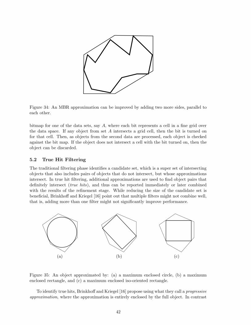
Figure 34: An MBR approximation can be improved by adding two more sides, parallel toeach other.

bitmap for one of the data sets, say A, where each bit represents a cell in a fine grid overthe data space. If any object from set A intersects a grid cell, then the bit is turned onfor that cell. Then, as objects from the second data are processed, each object is checkedagainst the bit map. If the object does not intersect a cell with the bit turned on, then theobject can be discarded.

5.2 True Hit Filtering

The traditional filtering phase identifies a candidate set, which is a super set of intersectingobjects that also includes pairs of objects that do not intersect, but whose approximationsintersect. In true hit filtering, additional approximations are used to find object pairs thatdefinitely intersect (true hits), and thus can be reported immediately or later combinedwith the results of the refinement stage. While reducing the size of the candidate set isbeneficial, Brinkhoff and Kriegel [16] point out that multiple filters might not combine well,that is, adding more than one filter might not significantly improve performance.

(a) (b) (c)

Figure 35: An object approximated by: (a) a maximum enclosed circle, (b) a maximumenclosed rectangle, and (c) a maximum enclosed iso-oriented rectangle.

To identify true hits, Brinkhoff and Kriegel [16] propose using what they call a progressiveapproximation, where the approximation is entirely enclosed by the full object. In contrast

42

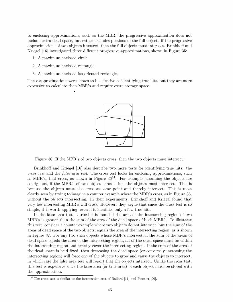
to enclosing approximations, such as the MBR, the progressive approximation does notinclude extra dead space, but rather excludes portions of the full object. If the progressiveapproximations of two objects intersect, then the full objects must intersect. Brinkhoff andKriegel [16] investigated three different progressive approximations, shown in Figure 35:

1. A maximum enclosed circle.

2. A maximum enclosed rectangle.

3. A maximum enclosed iso-oriented rectangle.

These approximations were shown to be effective at identifying true hits, but they are moreexpensive to calculate than MBR’s and require extra storage space.

Figure 36: If the MBR’s of two objects cross, then the two objects must intersect.

Brinkhoff and Kriegel [16] also describe two more tests for identifying true hits: thecross test and the false area test. The cross test looks for enclosing approximations, suchas MBR’s, that cross, as shown in Figure 3614. For example, assuming the objects arecontiguous, if the MBR’s of two objects cross, then the objects must intersect. This isbecause the objects must also cross at some point and thereby intersect. This is mostclearly seen by trying to imagine a counter example where the MBR’s cross, as in Figure 36,without the objects intersecting. In their experiments, Brinkhoff and Kriegel found thatvery few intersecting MBR’s will cross. However, they argue that since the cross test is sosimple, it is worth applying, even if it identifies only a few true hits.

In the false area test, a true-hit is found if the area of the intersecting region of twoMBR’s is greater than the sum of the area of the dead space of both MBR’s. To illustratethis test, consider a counter example where two objects do not intersect, but the sum of theareas of dead space of the two objects, equals the area of the intersecting region, as is shownin Figure 37. For any two such objects whose MBR’s intersect, if the sum of the areas ofdead space equals the area of the intersecting region, all of the dead space must be withinthe intersecting region and exactly cover the intersecting region. If the sum of the area ofthe dead space is held fixed, then decreasing the dead space (or conversely increasing theintersecting region) will force one of the objects to grow and cause the objects to intersect,in which case the false area test will report that the objects intersect. Unlike the cross test,this test is expensive since the false area (or true area) of each object must be stored withthe approximation.

14The cross test is similar to the intersection test of Ballard [11] and Peucker [90].

43

Dead space

(a)

Dead space

(b)

Intersecti ng region of MBR's.

(c)

Figure 37: The two objects in (a) and (b) do not intersect in (c). The false area test doesnot report a true hit since the area of the intersecting region only equals the sum of thedead space in (a) and (b), but is not greater than.

5.3 Non-Blocking Filtering

During the filtering phase, any algorithm will block while building an index, sorting thedata, or partitioning the data. No output will be produced while this occurs, which delaysoverall processing in a pipe-lined system [35]. This section first describes a variant of theindex nested-loop join (Section 3.2) which is non-blocking and then a method to make anyfiltering technique non-blocking.

procedure NON-BLOCKING_NESTED_LOOP_JOIN( combinedDataSets );

begin

spatialIndexA←INTIALIZE_DYNAMIC_SPATIAL_INDEX();

spatialIndexB←INTIALIZE_DYNAMIC_SPATIAL_INDEX();

for each dataElement ∈ combinedDataSets

if dataElement ∈ setA then

spatialIndexA.INSERT(dataElement)

intersections←spatialIndexB.SEARCH(dataElement)

else

spatialIndexB.INSERT(dataElement)

intersections←spatialIndexA.SEARCH(dataElement)

end if

REPORT(intersections)

end for each;

end;

Figure 38: A non-blocking index nested loop join allows results to be reported immediatelyand continuously.

The indexed nested-loop join in Section 3.2 blocks while it is building an index, thatis, it doesn’t produce any result pairs, which can slow processing in pipe-lined systems[35]. To overcome this limitation, Luo et al. [64] use a non-blocking variation of the indexnested-loop join so that some results are returned immediately. In the algorithm, shownin Figure 38, each data set is indexed using a dynamic index, such as an R-tree [40]. Adynamic index must be used, which can be less efficient than static indices, but static

44

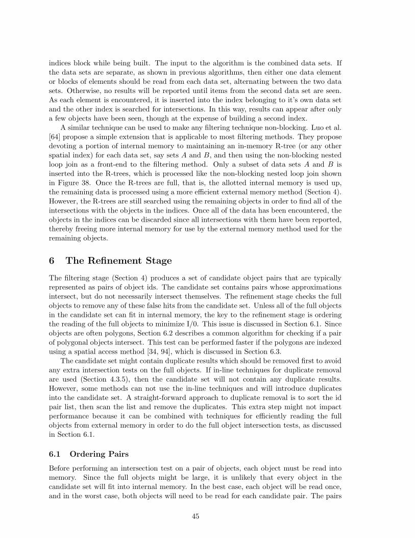
indices block while being built. The input to the algorithm is the combined data sets. Ifthe data sets are separate, as shown in previous algorithms, then either one data elementor blocks of elements should be read from each data set, alternating between the two datasets. Otherwise, no results will be reported until items from the second data set are seen.As each element is encountered, it is inserted into the index belonging to it’s own data setand the other index is searched for intersections. In this way, results can appear after onlya few objects have been seen, though at the expense of building a second index.

A similar technique can be used to make any filtering technique non-blocking. Luo et al.[64] propose a simple extension that is applicable to most filtering methods. They proposedevoting a portion of internal memory to maintaining an in-memory R-tree (or any otherspatial index) for each data set, say sets A and B, and then using the non-blocking nestedloop join as a front-end to the filtering method. Only a subset of data sets A and B isinserted into the R-trees, which is processed like the non-blocking nested loop join shownin Figure 38. Once the R-trees are full, that is, the allotted internal memory is used up,the remaining data is processed using a more efficient external memory method (Section 4).However, the R-trees are still searched using the remaining objects in order to find all of theintersections with the objects in the indices. Once all of the data has been encountered, theobjects in the indices can be discarded since all intersections with them have been reported,thereby freeing more internal memory for use by the external memory method used for theremaining objects.

6 The Refinement Stage

The filtering stage (Section 4) produces a set of candidate object pairs that are typicallyrepresented as pairs of object ids. The candidate set contains pairs whose approximationsintersect, but do not necessarily intersect themselves. The refinement stage checks the fullobjects to remove any of these false hits from the candidate set. Unless all of the full objectsin the candidate set can fit in internal memory, the key to the refinement stage is orderingthe reading of the full objects to minimize I/0. This issue is discussed in Section 6.1. Sinceobjects are often polygons, Section 6.2 describes a common algorithm for checking if a pairof polygonal objects intersect. This test can be performed faster if the polygons are indexedusing a spatial access method [34, 94], which is discussed in Section 6.3.

The candidate set might contain duplicate results which should be removed first to avoidany extra intersection tests on the full objects. If in-line techniques for duplicate removalare used (Section 4.3.5), then the candidate set will not contain any duplicate results.However, some methods can not use the in-line techniques and will introduce duplicatesinto the candidate set. A straight-forward approach to duplicate removal is to sort the idpair list, then scan the list and remove the duplicates. This extra step might not impactperformance because it can be combined with techniques for efficiently reading the fullobjects from external memory in order to do the full object intersection tests, as discussedin Section 6.1.

6.1 Ordering Pairs

Before performing an intersection test on a pair of objects, each object must be read intomemory. Since the full objects might be large, it is unlikely that every object in thecandidate set will fit into internal memory. In the best case, each object will be read once,and in the worst case, both objects will need to be read for each candidate pair. The pairs

45

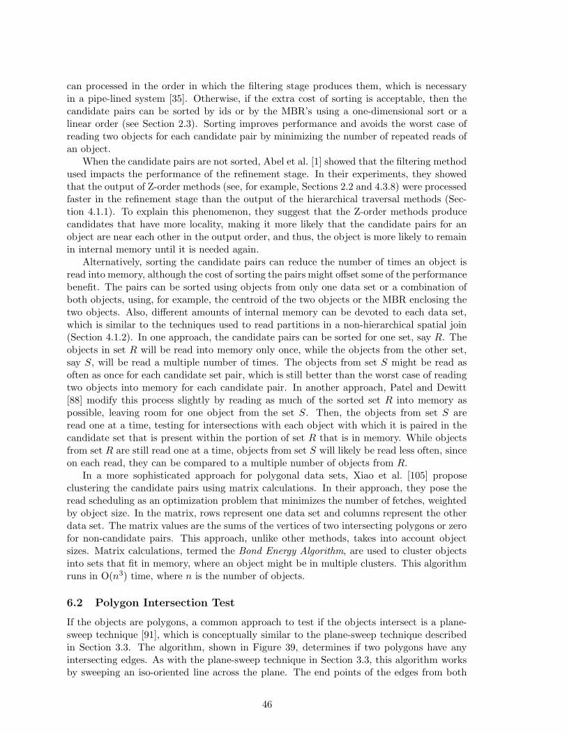
can processed in the order in which the filtering stage produces them, which is necessaryin a pipe-lined system [35]. Otherwise, if the extra cost of sorting is acceptable, then thecandidate pairs can be sorted by ids or by the MBR’s using a one-dimensional sort or alinear order (see Section 2.3). Sorting improves performance and avoids the worst case ofreading two objects for each candidate pair by minimizing the number of repeated reads ofan object.

When the candidate pairs are not sorted, Abel et al. [1] showed that the filtering methodused impacts the performance of the refinement stage. In their experiments, they showedthat the output of Z-order methods (see, for example, Sections 2.2 and 4.3.8) were processedfaster in the refinement stage than the output of the hierarchical traversal methods (Sec-tion 4.1.1). To explain this phenomenon, they suggest that the Z-order methods producecandidates that have more locality, making it more likely that the candidate pairs for anobject are near each other in the output order, and thus, the object is more likely to remainin internal memory until it is needed again.

Alternatively, sorting the candidate pairs can reduce the number of times an object isread into memory, although the cost of sorting the pairs might offset some of the performancebenefit. The pairs can be sorted using objects from only one data set or a combination ofboth objects, using, for example, the centroid of the two objects or the MBR enclosing thetwo objects. Also, different amounts of internal memory can be devoted to each data set,which is similar to the techniques used to read partitions in a non-hierarchical spatial join(Section 4.1.2). In one approach, the candidate pairs can be sorted for one set, say R. Theobjects in set R will be read into memory only once, while the objects from the other set,say S, will be read a multiple number of times. The objects from set S might be read asoften as once for each candidate set pair, which is still better than the worst case of readingtwo objects into memory for each candidate pair. In another approach, Patel and Dewitt[88] modify this process slightly by reading as much of the sorted set R into memory aspossible, leaving room for one object from the set S. Then, the objects from set S areread one at a time, testing for intersections with each object with which it is paired in thecandidate set that is present within the portion of set R that is in memory. While objectsfrom set R are still read one at a time, objects from set S will likely be read less often, sinceon each read, they can be compared to a multiple number of objects from R.

In a more sophisticated approach for polygonal data sets, Xiao et al. [105] proposeclustering the candidate pairs using matrix calculations. In their approach, they pose theread scheduling as an optimization problem that minimizes the number of fetches, weightedby object size. In the matrix, rows represent one data set and columns represent the otherdata set. The matrix values are the sums of the vertices of two intersecting polygons or zerofor non-candidate pairs. This approach, unlike other methods, takes into account objectsizes. Matrix calculations, termed the Bond Energy Algorithm, are used to cluster objectsinto sets that fit in memory, where an object might be in multiple clusters. This algorithmruns in O(n3) time, where n is the number of objects.

6.2 Polygon Intersection Test

If the objects are polygons, a common approach to test if the objects intersect is a plane-sweep technique [91], which is conceptually similar to the plane-sweep technique describedin Section 3.3. The algorithm, shown in Figure 39, determines if two polygons have anyintersecting edges. As with the plane-sweep technique in Section 3.3, this algorithm worksby sweeping an iso-oriented line across the plane. The end points of the edges from both

46

function EDGE_INTERSECTION_TEST(edgesA, edgesB,

MBRoverlap) : boolean

begin

allEdges←edgesA ∪ edgesB;

allEdgesInRegion←EDGES_IN_REGION(allEdges, MBRoverlap);

allEndPoints←DOUBLE_EDGES(allEdgesInRegion);

edgeList=SORT_BY_END_POINT(allEndPoints);

activeEdges←CREATE_SWEEP_STRUCTURE();

while edgeList 6= ∅ do

edge←edgeList.POP();

if edge is the beginning of the edge then

activeEdges.INSERT(edge);

edgeAbove←activeEdges.EDGE_ABOVE(edge);

edgeBelow←activeEdges.EDGE_BELOW(edge);

if INTERSECT(edge, edgeAbove)

OR INTERSECT(edge, edgeBelow) then

return true;

end if

else

if INTERSECT( edgeAbove, edgeBelow ) then

return true;

end if

activeEdges.REMOVE(edge);

end if

end loop

return false; /* No intersection detected. */end

Figure 39: A plane-sweep algorithm for detecting the intersection of simple polygons whoseMBR’s intersect.

polygons are the stopping points of the sweep line and the edges intersecting the sweepline form the active set. If the polygons do not have intersecting edges, one polygon couldbe contained within the other and a separate test for containment needs to be performed,which is described later.

The typical plane-sweep polygon intersection algorithm has been modified to improveits performance for the refinement stage using a technique of Brinkhoff et al. [19]. Sinceonly edges within the intersecting region of the MBRs of the two polygons could possiblyintersect, only those edges are used in the plane-sweep method. Any other edges are removedfrom consideration using the EDGES IN REGION function in the algorithm. For example, inFigure 40, edge e of polygon a is not contained in the intersecting region of the MBR’s andcould not possibly intersect polygon b.

The algorithm has also been simplified by assuming that the polygons are simple, that is,they do not intersect themselves. In the algorithm, as soon as an intersecting edge is found,the algorithm can report that the polygons intersect without checking if the intersectingedges belong to the same polygon because the polygons are simple 15.

15Becker et al. [12] review and propose algorithms for non-simple polygons and efficient algorithms for

47

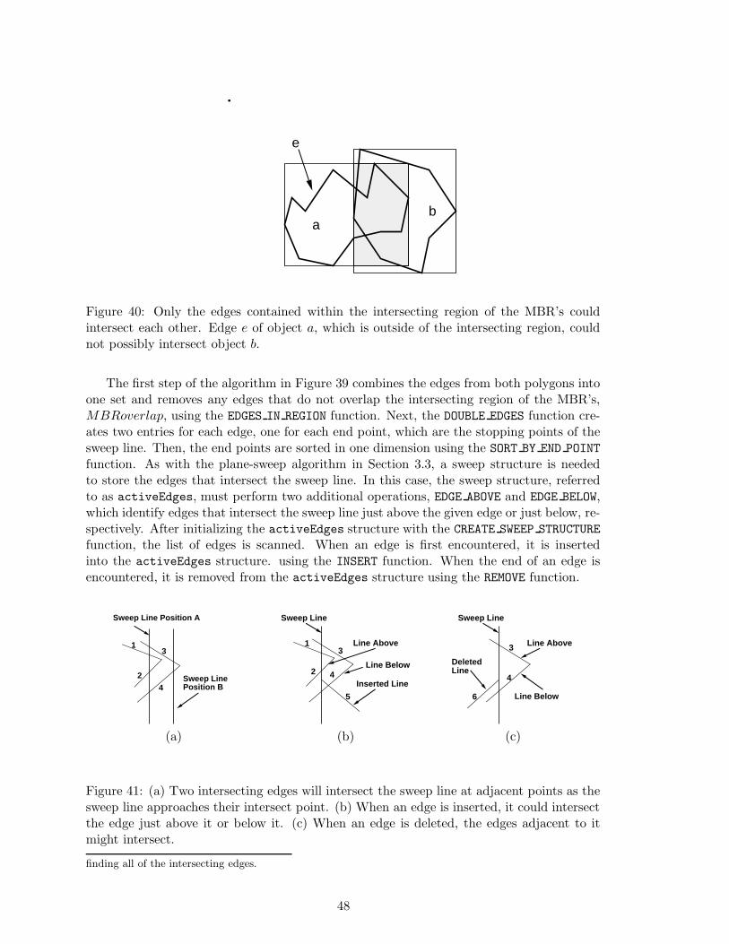
e

ab

Figure 40: Only the edges contained within the intersecting region of the MBR’s couldintersect each other. Edge e of object a, which is outside of the intersecting region, couldnot possibly intersect object b.

The first step of the algorithm in Figure 39 combines the edges from both polygons intoone set and removes any edges that do not overlap the intersecting region of the MBR’s,MBRoverlap, using the EDGES IN REGION function. Next, the DOUBLE EDGES function cre-ates two entries for each edge, one for each end point, which are the stopping points of thesweep line. Then, the end points are sorted in one dimension using the SORT BY END POINT

function. As with the plane-sweep algorithm in Section 3.3, a sweep structure is neededto store the edges that intersect the sweep line. In this case, the sweep structure, referredto as activeEdges, must perform two additional operations, EDGE ABOVE and EDGE BELOW,which identify edges that intersect the sweep line just above the given edge or just below, re-spectively. After initializing the activeEdges structure with the CREATE SWEEP STRUCTURE

function, the list of edges is scanned. When an edge is first encountered, it is insertedinto the activeEdges structure. using the INSERT function. When the end of an edge isencountered, it is removed from the activeEdges structure using the REMOVE function.

Sweep Line Position A

Sweep Line Position B

1

2

3

4

(a)

Sweep Line

Inserted Line

Line Above

Line Below

3

42

1

5

(b)

Sweep Line

Deleted Line

Line Above

Line Below

3

4

6

(c)

Figure 41: (a) Two intersecting edges will intersect the sweep line at adjacent points as thesweep line approaches their intersect point. (b) When an edge is inserted, it could intersectthe edge just above it or below it. (c) When an edge is deleted, the edges adjacent to itmight intersect.

finding all of the intersecting edges.

48

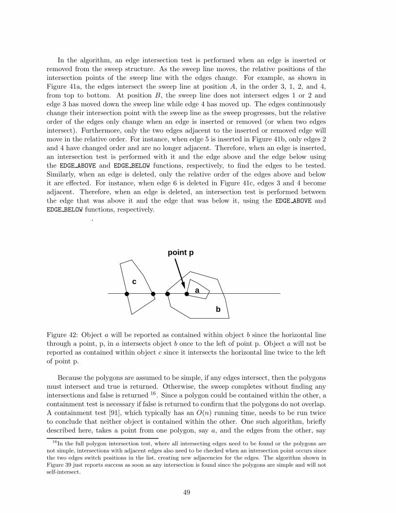
In the algorithm, an edge intersection test is performed when an edge is inserted orremoved from the sweep structure. As the sweep line moves, the relative positions of theintersection points of the sweep line with the edges change. For example, as shown inFigure 41a, the edges intersect the sweep line at position A, in the order 3, 1, 2, and 4,from top to bottom. At position B, the sweep line does not intersect edges 1 or 2 andedge 3 has moved down the sweep line while edge 4 has moved up. The edges continuouslychange their intersection point with the sweep line as the sweep progresses, but the relativeorder of the edges only change when an edge is inserted or removed (or when two edgesintersect). Furthermore, only the two edges adjacent to the inserted or removed edge willmove in the relative order. For instance, when edge 5 is inserted in Figure 41b, only edges 2and 4 have changed order and are no longer adjacent. Therefore, when an edge is inserted,an intersection test is performed with it and the edge above and the edge below usingthe EDGE ABOVE and EDGE BELOW functions, respectively, to find the edges to be tested.Similarly, when an edge is deleted, only the relative order of the edges above and belowit are effected. For instance, when edge 6 is deleted in Figure 41c, edges 3 and 4 becomeadjacent. Therefore, when an edge is deleted, an intersection test is performed betweenthe edge that was above it and the edge that was below it, using the EDGE ABOVE andEDGE BELOW functions, respectively.

a

b

c

point p

Figure 42: Object a will be reported as contained within object b since the horizontal linethrough a point, p, in a intersects object b once to the left of point p. Object a will not bereported as contained within object c since it intersects the horizontal line twice to the leftof point p.

Because the polygons are assumed to be simple, if any edges intersect, then the polygonsmust intersect and true is returned. Otherwise, the sweep completes without finding anyintersections and false is returned 16. Since a polygon could be contained within the other, acontainment test is necessary if false is returned to confirm that the polygons do not overlap.A containment test [91], which typically has an O(n) running time, needs to be run twiceto conclude that neither object is contained within the other. One such algorithm, brieflydescribed here, takes a point from one polygon, say a, and the edges from the other, say

16In the full polygon intersection test, where all intersecting edges need to be found or the polygons arenot simple, intersections with adjacent edges also need to be checked when an intersection point occurs sincethe two edges switch positions in the list, creating new adjacencies for the edges. The algorithm shown inFigure 39 just reports success as soon as any intersection is found since the polygons are simple and will notself-intersect.

49

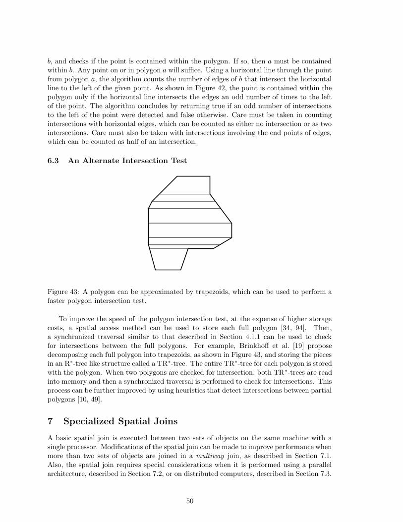
b, and checks if the point is contained within the polygon. If so, then a must be containedwithin b. Any point on or in polygon a will suffice. Using a horizontal line through the pointfrom polygon a, the algorithm counts the number of edges of b that intersect the horizontalline to the left of the given point. As shown in Figure 42, the point is contained within thepolygon only if the horizontal line intersects the edges an odd number of times to the leftof the point. The algorithm concludes by returning true if an odd number of intersectionsto the left of the point were detected and false otherwise. Care must be taken in countingintersections with horizontal edges, which can be counted as either no intersection or as twointersections. Care must also be taken with intersections involving the end points of edges,which can be counted as half of an intersection.

6.3 An Alternate Intersection Test

Figure 43: A polygon can be approximated by trapezoids, which can be used to perform afaster polygon intersection test.

To improve the speed of the polygon intersection test, at the expense of higher storagecosts, a spatial access method can be used to store each full polygon [34, 94]. Then,a synchronized traversal similar to that described in Section 4.1.1 can be used to checkfor intersections between the full polygons. For example, Brinkhoff et al. [19] proposedecomposing each full polygon into trapezoids, as shown in Figure 43, and storing the piecesin an R∗-tree like structure called a TR∗-tree. The entire TR∗-tree for each polygon is storedwith the polygon. When two polygons are checked for intersection, both TR∗-trees are readinto memory and then a synchronized traversal is performed to check for intersections. Thisprocess can be further improved by using heuristics that detect intersections between partialpolygons [10, 49].

7 Specialized Spatial Joins

A basic spatial join is executed between two sets of objects on the same machine with asingle processor. Modifications of the spatial join can be made to improve performance whenmore than two sets of objects are joined in a multiway join, as described in Section 7.1.Also, the spatial join requires special considerations when it is performed using a parallelarchitecture, described in Section 7.2, or on distributed computers, described in Section 7.3.

50

Specialized hardware can also be used to improve performance. Sun et al. [98] proposetaking advantage of graphics hardware to perform efficient spatial joins. They suggest as-signing a different color to each data set and then letting the graphics hardware renderthe data sets for the screen. Then, the frame buffer can be searched for regions contain-ing a combination of the colors, which indicates intersecting objects. From an analyticalstandpoint, the algorithm will be worse because of the scan of the frame buffer, but theoverall performance will be improved due to the advanced hardware. However, the graphicshardware typically only works on convex polygons and only a limited resolution can beachieved, leading to false hits that still need to be refined. Additionally, Sun et al. proposeusing a similar approach to determine if two polygons intersect. In this case, the edges ofone polygon are colored one way and the other polygon’s edges are colored differently.

In another specialized situation, as mentioned by Gunther [36], if the data set is notupdated often and speed is critical, a spatial join index [93] can be used. All of the inter-secting objects are found ahead of time and the resulting pairs of ids are stored in an index.A spatial join algorithm must be used though, to create the original set of results pairs.

7.1 Multiway Joins and Query Plans

A complex query could contain multiple spatial joins. As an example, consider the query– find all regions between 500 meters and 700 meters above sea level that receive 10 to 15centimeters of rainfall and are in a forested area. This query requires a spatial join to findthe intersecting regions of rainfall and elevation and also the intersection with land type(forest). This query can be answered by performing a spatial join between any two of thedata sets and joining the results with the third data set. The intermediate results are theintersecting regions of the result candidate set, which is then joined with the third data set.In the example, rainfall and elevation can be joined, creating a new data set that representsregions with 10 to 15 centimeters of rainfall and are between 500 and 700 meters above sealevel. This intermediate data set is then joined with land type data to create the final resultof regions.

The previous example illustrates a query with mutual intersection between the datasets. A spatial query might not require that the data sets mutually intersect. For example,the query – find all roads that cross a river and a railroad track – does not require thatthe river and railroad track in a result triplet intersect. In Figure 44a, the three objectshave a mutually intersecting region, but in Figure 44b, each object pair-wise intersects.Furthermore, not all data sets in the query might have a relation. For instance, as shownin Figure 44c, the query could only require that objects from data set B intersect an objectfrom both A and C, but no restriction is placed on intersections between A and C, suchas with the road, river, and railroad example. In general, a multiway spatial query can berepresented by a graph, as shown in Figure 45, in which n-ary relations are used to representmutually intersecting regions. For instance, in Figure 45, objects from A, B, and C arerequired to mutually intersect, as in Figure 44a, as opposed to objects D, F , and G, whichare only required to pair-wise intersect, as in Figure 44b.

As mentioned, a multiway spatial join can be solved by joining two data sets at atime and creating intermediate data sets. Furthermore, traditional database optimizationapproaches [35] that order the pair-wise joins to efficiently solve the query can be used[66]. To do this, selectivity estimates (Section 7.4) are required in order to efficientlydetermine which relation to solve first, typically solving the relation that produces thesmallest intermediate result first.

51

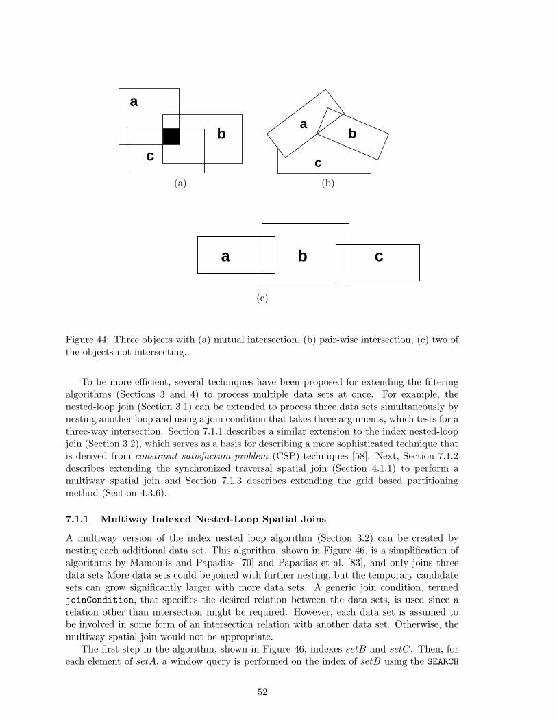
b

a

c

(a)

ba

c(b)

ba c

(c)

Figure 44: Three objects with (a) mutual intersection, (b) pair-wise intersection, (c) two ofthe objects not intersecting.

To be more efficient, several techniques have been proposed for extending the filteringalgorithms (Sections 3 and 4) to process multiple data sets at once. For example, thenested-loop join (Section 3.1) can be extended to process three data sets simultaneously bynesting another loop and using a join condition that takes three arguments, which tests for athree-way intersection. Section 7.1.1 describes a similar extension to the index nested-loopjoin (Section 3.2), which serves as a basis for describing a more sophisticated technique thatis derived from constraint satisfaction problem (CSP) techniques [58]. Next, Section 7.1.2describes extending the synchronized traversal spatial join (Section 4.1.1) to perform amultiway spatial join and Section 7.1.3 describes extending the grid based partitioningmethod (Section 4.3.6).

7.1.1 Multiway Indexed Nested-Loop Spatial Joins

A multiway version of the index nested loop algorithm (Section 3.2) can be created bynesting each additional data set. This algorithm, shown in Figure 46, is a simplification ofalgorithms by Mamoulis and Papadias [70] and Papadias et al. [83], and only joins threedata sets More data sets could be joined with further nesting, but the temporary candidatesets can grow significantly larger with more data sets. A generic join condition, termedjoinCondition, that specifies the desired relation between the data sets, is used since arelation other than intersection might be required. However, each data set is assumed tobe involved in some form of an intersection relation with another data set. Otherwise, themultiway spatial join would not be appropriate.

The first step in the algorithm, shown in Figure 46, indexes setB and setC. Then, foreach element of setA, a window query is performed on the index of setB using the SEARCH

52

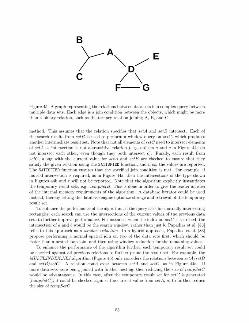
BA

CD

E

GF

Figure 45: A graph representing the relations between data sets in a complex query betweenmultiple data sets. Each edge is a join condition between the objects, which might be morethan a binary relation, such as the ternary relation joining A, B, and C.

method. This assumes that the relation specifies that setA and setB intersect. Each ofthe search results from setB is used to perform a window query on setC, which producesanother intermediate result set. Note that not all elements of setC need to intersect elementsof setA as intersection is not a transitive relation (e.g., objects a and c in Figure 44c donot intersect each other, even though they both intersect c). Finally, each result fromsetC, along with the current value for setA and setB are checked to ensure that theysatisfy the given relation using the SATISFIED function, and if so, the values are reported.The SATISFIED function ensures that the specified join condition is met. For example, ifmutual intersection is required, as in Figure 44a, then the intersections of the type shownin Figures 44b and c will not be reported. Note that the algorithm explicitly instantiatesthe temporary result sets, e.g., tempSetB. This is done in order to give the reader an ideaof the internal memory requirements of the algorithm. A database iterator could be usedinstead, thereby letting the database engine optimize storage and retrieval of the temporaryresult set.

To enhance the performance of the algorithm, if the query asks for mutually intersectingrectangles, each search can use the intersections of the current values of the previous datasets to further improve performance. For instance, when the index on setC is searched, theintersection of a and b would be the search window, rather than just b. Papadias et al. [83]refer to this approach as a window reduction. In a hybrid approach, Papadias et al. [83]propose performing a normal spatial join on two of the data sets first, which should befaster than a nested-loop join, and then using window reduction for the remaining values.

To enhance the performance of the algorithm further, each temporary result set couldbe checked against all previous relations to further prune the result set. For example, theMULTI INDEX NLJ algorithm (Figure 46) only considers the relations between setA/setBand setB/setC. A relation could exist between setA and setC, as in Figure 44a. Ifmore data sets were being joined with further nesting, then reducing the size of tempSetC

would be advantageous. In this case, after the temporary result set for setC is generated(tempSetC), it could be checked against the current value from setA, a, to further reducethe size of tempSetC.

53

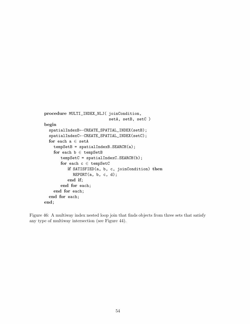
procedure MULTI_INDEX_NLJ( joinCondition,

setA, setB, setC )

begin

spatialIndexB←CREATE_SPATIAL_INDEX(setB);

spatialIndexC←CREATE_SPATIAL_INDEX(setC);

for each a ∈ setA

tempSetB = spatialIndexB.SEARCH(a);

for each b ∈ tempSetB

tempSetC = spatialIndexC.SEARCH(b);

for each c ∈ tempSetC

if SATISFIED(a, b, c, joinCondition) then

REPORT(a, b, c, d);

end if;

end for each;

end for each;

end for each;

end;

Figure 46: A multiway index nested loop join that finds objects from three sets that satisfyany type of multiway intersection (see Figure 44).

54

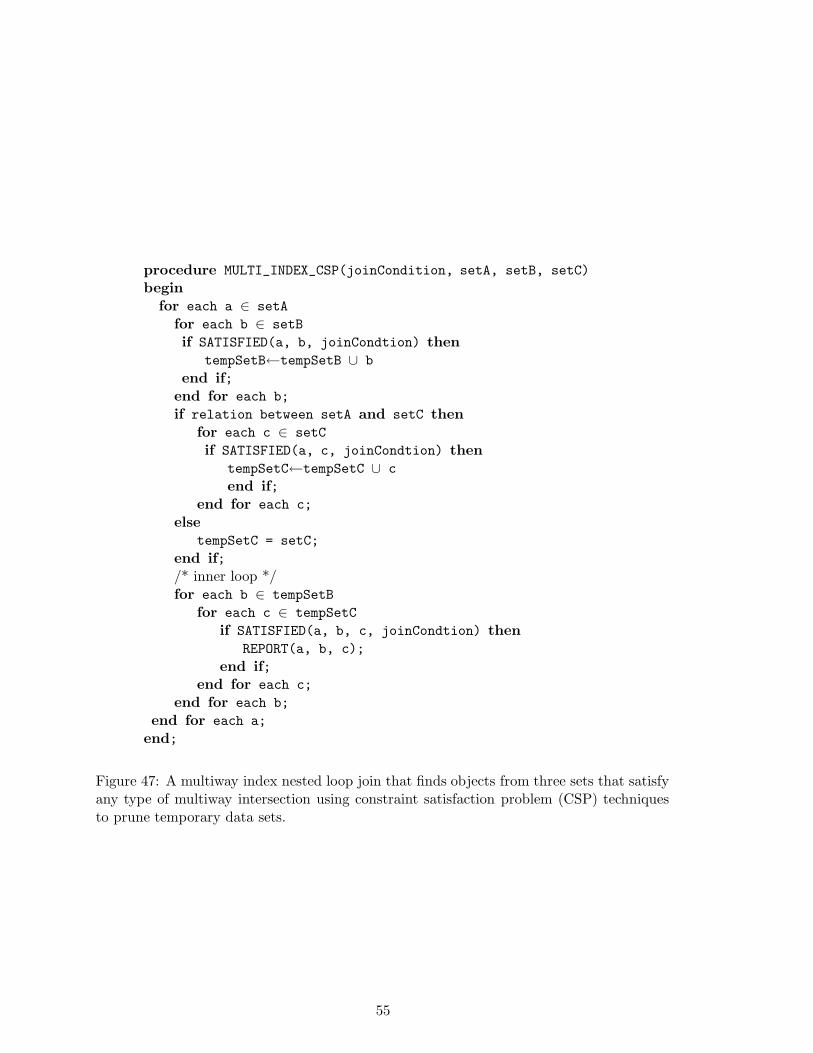
procedure MULTI_INDEX_CSP(joinCondition, setA, setB, setC)

begin

for each a ∈ setA

for each b ∈ setB

if SATISFIED(a, b, joinCondtion) then

tempSetB←tempSetB ∪ b

end if;

end for each b;

if relation between setA and setC then

for each c ∈ setC

if SATISFIED(a, c, joinCondtion) then

tempSetC←tempSetC ∪ c

end if;

end for each c;

else

tempSetC = setC;

end if;

/* inner loop */for each b ∈ tempSetB

for each c ∈ tempSetC

if SATISFIED(a, b, c, joinCondtion) then

REPORT(a, b, c);

end if;

end for each c;

end for each b;

end for each a;

end;

Figure 47: A multiway index nested loop join that finds objects from three sets that satisfyany type of multiway intersection using constraint satisfaction problem (CSP) techniquesto prune temporary data sets.

55

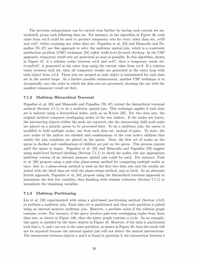
The previous enhancement can be carried even further by having each current set im-mediately prune each following data set. For instance, in the algorithm in Figure 46, eachvalue from setA could be used to produce temporary sets for every other data set, setB

and setC, before scanning any other data set. Papadias et al. [83] and Mamoulis and Pa-padias [70, 67] use this approach to solve the multiway spatial join, which is a constraintsatisfaction problem (CSP) technique [58] called multi-level forward checking. In the CSPapproach, temporary result sets are generated as soon as possible. In this algorithm, shownin Figure 47, if a relation exists between setA and setC, then a temporary result set,tempSetC, is generated in the outer loop using the current value from setA. If a relationexists between each set, then all temporary results are generated in the outer loop witheach object from setA. These sets are pruned as each object is instantiated for each dataset in the nested loops. As a further possible enhancement, another CSP technique is todynamically vary the order in which the data sets are processed, choosing the one with thesmallest temporary result set first.

7.1.2 Multiway Hierarchical Traversal

Papadias et al. [83] and Mamoulis and Papadias [70, 67] extend the hierarchical traversalmethod (Section 4.1.1) to do a multiway spatial join. This technique applies if each dataset is indexed using a hierarchical index, such as an R-tree [40]. For two data sets, theoriginal method compares overlapping nodes of the two indices. If the nodes are leaves,the intersecting objects within the node are reported, else the intersecting child node pairsare placed on a priority queue to be processed later. To do a multiway join, the queue ismodified to hold multiple nodes, one from each data set, instead of pairs. To start, theroot nodes of the indices are checked and combinations of the root node’s children thatsatisfy the join condition are placed on the queue. Next, the first set of nodes on thequeue is checked and combinations of children are put on the queue. This process repeatsuntil the queue is empty. Papadias et al. [83] and Mamoulis and Papadias [70] suggestusing multi-level forward checking (Section 7.1.1) to check the nodes, but any appropriatemultiway version of an internal memory spatial join could be used. For instance, Parket al. [86] propose using a pair-wise plane-sweep method for comparing multiple nodes atonce, that is, a plane-sweep method is used on the first two data sets and the results arejoined with the third data set with the plane-sweep method, and so forth. As an alternatehybrid approach, Papadias et al. [84] propose using the hierarchical traversal approach toinstantiate the first few variables, then finishing with window reduction (Section 7.1.1) toinstantiate the remaining variables.

7.1.3 Multiway Partitioning

Lin et al. [59] experimented with using a grid-based partitioning method (Section 4.3.6)to perform a multiway join. Each data set is partitioned and then each partition is joinedusing an internal memory multiway join. However, a problem arises if the relation graphcontains cycles. For instance, if the query involves pair-wise overlapping tuples from threedata sets, as shown in Figure 44b, then the query graph contains a cycle. As an example,this query is satisfied by the three objects in Figure 48. However, if the data is partitionedsuch that a, b, and c are not in the same partition, as shown in Figure 48, then the result willnot be reported because the internal spatial join will not detect the mutual intersections.The intersection between objects a and b is found in partition 2, the intersection between b

56

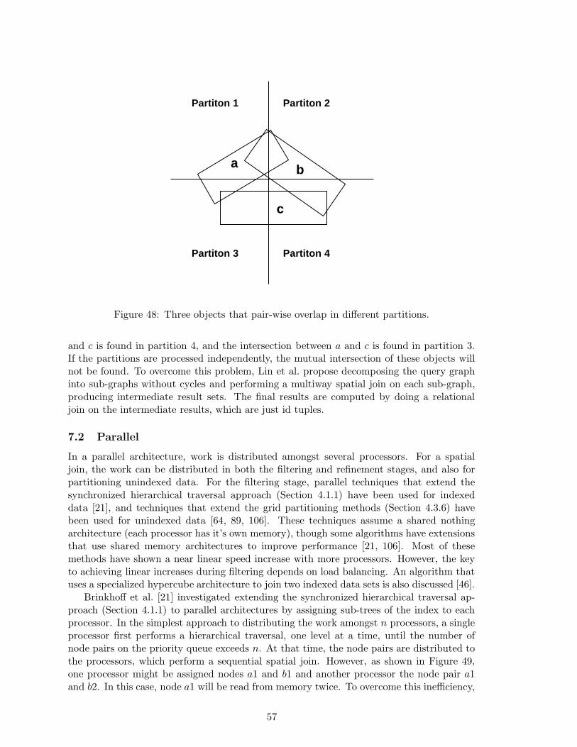
ba

c

Partiton 1 Partiton 2

Partiton 3 Partiton 4

Figure 48: Three objects that pair-wise overlap in different partitions.

and c is found in partition 4, and the intersection between a and c is found in partition 3.If the partitions are processed independently, the mutual intersection of these objects willnot be found. To overcome this problem, Lin et al. propose decomposing the query graphinto sub-graphs without cycles and performing a multiway spatial join on each sub-graph,producing intermediate result sets. The final results are computed by doing a relationaljoin on the intermediate results, which are just id tuples.

7.2 Parallel

In a parallel architecture, work is distributed amongst several processors. For a spatialjoin, the work can be distributed in both the filtering and refinement stages, and also forpartitioning unindexed data. For the filtering stage, parallel techniques that extend thesynchronized hierarchical traversal approach (Section 4.1.1) have been used for indexeddata [21], and techniques that extend the grid partitioning methods (Section 4.3.6) havebeen used for unindexed data [64, 89, 106]. These techniques assume a shared nothingarchitecture (each processor has it’s own memory), though some algorithms have extensionsthat use shared memory architectures to improve performance [21, 106]. Most of thesemethods have shown a near linear speed increase with more processors. However, the keyto achieving linear increases during filtering depends on load balancing. An algorithm thatuses a specialized hypercube architecture to join two indexed data sets is also discussed [46].

Brinkhoff et al. [21] investigated extending the synchronized hierarchical traversal ap-proach (Section 4.1.1) to parallel architectures by assigning sub-trees of the index to eachprocessor. In the simplest approach to distributing the work amongst n processors, a singleprocessor first performs a hierarchical traversal, one level at a time, until the number ofnode pairs on the priority queue exceeds n. At that time, the node pairs are distributed tothe processors, which perform a sequential spatial join. However, as shown in Figure 49,one processor might be assigned nodes a1 and b1 and another processor the node pair a1and b2. In this case, node a1 will be read from memory twice. To overcome this inefficiency,

57

Index Node a1

Index Node b1 Index Node b2

Figure 49: Objects in multiple partitions might be read from memory multiple times.

Brinkhoff et al. propose using global buffers (in a shared memory architecture) so that oneprocessor can access a node that another processor has read into internal memory. However,this approach does incur extra communications to synchronize usage of the buffers. Addi-tionally, the workloads might not be balanced since the processing time for each sub-treecould be different. Rather than assigning all of the node pairs from the queue at once,Brinkhoff et al. suggest assigning only one node pair at a time to each processor. Once aprocessor finishes with one node pair, another is requested while the queue is not empty.When the queue is empty, they further suggest that one processor can share the work ofanother processor by taking node pairs from another processor’s local queue, i.e., sub-treesof the original sub-trees.

For unindexed data, Zhou et al. [106] adapt the variation of the grid partitioning method(Section 4.3.6) that physically creates the tiles. In their approach, the random data isevenly divided amongst the n processors, which then partition the data using the sametiling scheme. Then, with the sizes of the tiles known, a single processor determines themerging of tiles into n partitions using a Z-order merge, creating, on average, an even loaddistribution amongst the processors. Next, each processor is assigned a partition and thedata is redistributed appropriately. Finally, each processor filters the data using a sequentialspatial join filtering technique. Both Patel and Dewitt [89] and Luo et al. [64] investigated asimilar approach. Rather than physically tiling the data, though, they both use the virtualtiling method (Section 4.3.6), relying on a good hash function to distribute the data evenly.

For parallel refinement, each processor could refine the candidate pairs it produces.However, Zhou et al. [106] point out that it is difficult without much selectivity informationto balance the number of candidates produced by each processor during the filtering stage.If the candidate pairs are redistributed, then the workload for refinement can be close tooptimal since the number of vertices in each polygon are good estimates of performance.Like sequential refinement, performance can be improved by ordering the candidate set tominimize the number of times each full object is read. Zhou et al. argue that an efficientapproach is to use one processor to sort the candidates into a linear order, and then assignthe candidates to each processor in a round-robin fashion. Each processor will be process-ing candidate pairs that are near each other (exhibiting locality), allowing for a greaterchance that an object only needs to be read into internal memory once (assuming a sharedmemory architecture), rather than continually reading some of the same objects through-out refinement. Zhou et al. took the approach of assigning full objects to processors, which

58

are responsible for reading the object into memory and distributing the object to otherprocessors. They found that the redistribution costs are negligible.

Hoel and Samet [46] describe parallel algorithms for PMR bucket quad-trees [73] andR-trees [40] using a specialized hypercube architecture. The algorithms require that thedata fit in memory, but result in extremely fast algorithms. In their quad-tree approach,regions of one of the quad-trees are associated with half of the nodes (processors), termedthe source nodes, and corresponding regions of the other quad-tree are associated with theother nodes, termed the target nodes. Each quad-tree is assumed to cover the same area, andthus, because of the regular decomposition, there is a one-to-one correspondence betweensource nodes and target nodes. The source nodes send their objects to the target nodes,which check for intersections. Hoel and Samet also describe a similar algorithm for R-treesin which the index nodes of the R-tree are associated with the processor nodes. However,because of the irregular decomposition, each source node will be associated with multipletarget nodes, dramatically increasing the communication costs and slowing the join.

7.3 Distributed

Abel et al. [2] show how to combine the semi-join [72] concept for distributed join processingand the filter-and-refine approach for spatial join processing. Given two sets of objects, R

and S, that are at different locations (physically distributed), they send the MBR’s of setR to the S location and filter the objects there. Then, they send the full objects from S

that are in the candidate set to R’s location to perform the refinement step. Tan et al. [99]point out that unlike a relational semi-join [82], where the transmission cost is dominant,the processing cost can be just as large of a factor for spatial joins.

Mamoulis et al. [65] explore the distributed spatial join problem in which the dataresides on different servers between which there is no communication and the servers willnot perform a spatial join. This would be the case if the servers are commercially ownedand contain proprietary data. Additionally, it is assumed that the servers will not providestatistics on the data. In this case, the spatial join must be performed at a third, possiblysmall, site, such as a mobile device. They point out that any processing at the dataserver sites is relatively inexpensive compared to a mobile device. Therefore, as much workas possible should be done on the data servers, such as running queries to build usefulstatistics on the data. To do the spatial join, they propose a grid-based partitioning spatialjoin (Section 4.3.6) and use the detailed statistics to determine the best grid such that datafits within the available internal memory. The statistics are also used to identify emptyregions in a data set for which no spatial join needs to be performed, thus saving valuabletransmission costs.

7.4 Selectivity Estimation

Techniques for estimating the selectivity of a spatial join are important as an aid for ana-lyzing spatial join algorithms, for use in optimizers, and as a data mining tool. Gunther etal. [37] have shown that along with the size of the data set, selectivity is crucial in determin-ing the performance of an algorithm. Optimizers assist a database engine in determiningthe order of operations in a complex query. Also, selectivity estimates could play a rollin determining which spatial join algorithm to use. For instance, a very dense data set inwhich nearly every pair is reported, could be computed faster using the simple nested loopjoin (Section 3.1), rather than a more complex algorithm with a large overhead. For data

59

mining applications, selectivity estimates can give approximate answers to queries, whichcan be used to rule out hypothesis [14].

For uniform data sets in two dimensions, a rudimentary estimate of the selectivity forthe filtering stage of a spatial join can be derived from the probability that two averagesized rectangles overlap [4]. Given that both sets are enclosed in a universe of finite area,which is represented as TotalArea, the chances that two rectangles with widths wa and wb

and heights ha and hb are:

(wa + wb) · (ha + hb)

TotalArea=

areaa + areab + (wa · hb) + (wb · ha)

TotalArea, (2)

where areaa and areab are the areas of two rectangles 17. To derive a selectivity estimatefor a spatial join between two uniform data sets, the average sizes of the rectangles in thetwo sets A and B are substituted into Equation 2. Then, the selectivity is approximately:

areaA + areab + (wA · hB) + (wB · hA)

TotalArea. (3)

However, the situation is more complicated for non-uniform data sets. Mamoulis andPapadias [68] and An et al. [3] propose using a two-dimensional histogram on each dataset, which can be a grid with occupancy counts. Within each grid cell, the selectivityestimate for uniform data sets, Equation 3, can be applied. The finer the histogram, themore accurate the results will be. The results for each cell are then combined to get anoverall estimate of selectivity. An et al. also studied sampling techniques and proposed anovel technique for estimating intersections within a grid cell by counting the number ofsides and corners of rectangles within each grid cell.

In another approach, working with points data sets, Belussi and Faloutsos [14] expressedthe selectivity of a self-spatial join in terms of a fractal dimension. Since the data is points,the spatial join finds all pairs of points within a distance ε, which is expressed as nb(ε), andis analogous to the average number of intersecting pairs, that is, the selectivity of the spatialjoin 18. The average number of nearby, or neighboring, points captures information aboutthe distribution of data. If the data is clustered, then the average number of neighborsincreases. The problem, then, is to find a good estimate of the number of neighbors. To dothis, Belussi and Faloutsos use the fractal correlation dimension D2, which is a characteristicof the data set, and calculate the average number of neighbors as:

nb(ε) = (n− 1) · (2 · ε)D2 , (4)

where n is the number of points. Using this equation, the selectivity of a self-spatialjoin is estimated as (2 · ε)D2 . The correlation dimension, D2, can be calculated in O(n ·log(n)) time [14] or even in constant time according to Faloutsos et al. [30], who describealgorithms for efficiently calculating the correlation dimension for a given data set and showthe effectiveness of the calculation for predicting the selectivity of a self-spatial join 19.

17Equation 2 assumes that the space wraps around and doesn’t account for the need for rectangles to bewithin the spaces boundaries. However, the difference is negligible if the rectangle is a small fraction of thespace. Also, a minus one value is also dropped from the sums, for simplicity.

18Though, nb(ε) as defined by Belussi and Faloutsos [14] is the number of points within a circle, here,their generalization to other shapes is used. In this case, a rectangle.

19Faloutsos et al. [30] use the formula K · rP for selectivity, instead of Equation 3, where r replaces 2 · ε

and P replaces D2, and they also use the multiplier K.

60

8 Concluding Remarks

This article provides an in-depth survey and analysis of the various techniques used toperform a spatial join using a filter-and-refine approach in which complex objects are ap-proximated, typically by a minimum bounding rectangle. The approximations are joined,producing a candidate set which is refined to produce the final results using the full objects.We examined various techniques for performing a spatial join using the available internalmemory, using either nested loop joins, indexed nested loop joins, or variants of the plane-sweep technique. If there is insufficient internal memory, then external memory memorycan be used to process larger data sets. We examined cases where the data is indexed ornot indexed. If the data sets are indexed, then overlapping data pages can be read in apredetermined order or the two indices can be traversed synchronously if the indices arehierarchical. Pairs of overlapping data pages are joined using internal memory techniques.Alternatively, if the data is not indexed, then the data can be partitioned using a variety oftechniques, and then overlapping partition pairs can be joined using internal memory tech-niques. We also examined the techniques and issues involved with refining the candidateset produced during the filtering stage. Finally, we looked at spatial joins in a variety ofsituations: multiway spatial joins, parallel spatial joins, and distributed spatial joins.

Our goal was to provide a guide as to what techniques work best in particular situations.However, we are unable to conclusively determine the choice of techniques since we feelthat the experiments comparing techniques are inconclusive and can easily be skewed bythe choice of experimental data or details of implementation. We hope that this surveyilluminates some of these issues and motivates further analysis and experimentation.

References

[1] D. J. Abel, V. Gaede, R. Power, and X. Zhou. Caching strategies for spatial joins.GeoInformatica, 3(1):33–59, June 1999.

[2] D. J. Abel, B. C. Ooi, K.-L. Tan, R. Power, and J. X. Yu. Spatial join strategies indistributed spatial DBMS. In M. J. Egenhofer and J. R. Herring, editors, Advances inSpatial Databases—4th International Symposium, SSD’95, vol. 951 of Springer-VerlagLecture Notes in Computer Science, pages 348–367, Portland, ME, August 1995.

[3] N. An, Z.-Y. Yang, and A. Sivasubramaniam. Selectivity estimation for spatial joins.In Proceedings of the 17th International Conference on Data Engineering, pages 368–375, Heidelberg, Germany, April 2001.

[4] W. G. Aref and H. Samet. A cost model for query optimization using R-trees. InN. Pissinou and K. Makki, editors, Proceedings of the 2nd ACM Workshop on Geo-graphic Information Systems, pages 60–67, Gaithersburg, MD, December 1994.

[5] W. G. Aref and H. Samet. Hashing by proximity to process duplicates in spatialdatabases. In Proceedings of the 3rd International Conference on Information andKnowledge Management (CIKM), pages 347–354, Gaithersburg, MD, December 1994.

[6] W. G. Aref and H. Samet. The spatial filter revisited. In T. C. Waugh and R. G.Healey, editors, Proceedings of the 6th International Symposium on Spatial Data Han-dling, pages 190–208, Edinburgh, Scotland, September 1994. International Geograph-

61

ical Union Commission on Geographic Information Systems, Association for Geo-graphical Information.

[7] W. G. Aref and H. Samet. Cascaded spatial join algorithms with spatially sorted out-put. In S. Shekhar and P. Bergougnoux, editors, Proceedings of the 4th ACM Work-shop on Geographic Information Systems, pages 17–24, Gaithersburg, MD, November1996.

[8] L. Arge, O. Procopiuc, S. Ramaswamy, T. Suel, J. Vahrenhold, and J. S. Vitter. Aunified approach for indexed and non-indexed spatial joins. In C. Zaniolo, P. C. Lock-emann, M. H. Scholl, and T. Grust, editors, Proceedings of the 7th International Con-ference on Extending Database Technology—EDBT 2000, vol. 1777 of Springer-VerlagLecture Notes in Computer Science, pages 413–429, Konstanz, Germany, March 2000.

[9] L. Arge, O. Procopiuc, S. Ramaswamy, T. Suel, and J. S. Vitter. Scalable sweeping-based spatial join. In A. Gupta, O. Shmueli, and J. Widom, editors, Proceedings ofthe 24th International Conference on Very Large Data Bases (VLDB), pages 570–581,New York, August 1998.

[10] W.M. Badawy and W.G. Aref. On local heuristics to speed up polygon-polygonintersection tests. In Claudia Bauzer Medeiros, editor, Proceedings of the 7th ACMInternational Symposium on Advances in Geographic Information Systems, pages 97–102, Kansas City, MO, November 1999.

[11] D. H. Ballard. Strip trees: a hierarchical representation for curves. Communicationsof the ACM, 24(5):310–321, May 1981. Also see corrigendum, Communications of theACM, 25(3):213, March 1982.

[12] L. Becker, A. Giesen, K. Hinrichs, and J. Vahrenhold. Algorithms for performingpolygonal map overlay and spatial join on massive data set. In R. H. Guting, D. Papa-dias, and F. H. Lochovsky, editors, Advances in Spatial Databases—6th InternationalSymposium, SSD’99, vol. 1651 of Springer-Verlag Lecture Notes in Computer Science,pages 270–285, Hong Kong, China, July 1999.

[13] L. Becker, K. Hinrichs, and U. Finke. A new algorithm for computing joins with gridfiles. In Proceedings of the 9th IEEE International Conference on Data Engineering,pages 190–197, Vienna, Austria, April 1993.

[14] A. Belussi and C. Faloutsos. Estimating the selectivity of spatial queries using the‘correlation’ fractal dimension. In U. Dayal, P. M. D. Gray, and S. Nishio, editors,Proceedings of the 21st International Conference on Very Large Data Bases (VLDB),pages 299–310, Zurich, Switzerland, September 1995.

[15] J. L. Bentley. Multidimensional binary search trees used for associative searching.Communications of the ACM, 18(9):509–517, September 1975.

[16] T. Brinkhoff and H.-P. Kriegel. Approximations for a multi-step processing of spatialjoins. In J. Nievergelt, T. Roos, H.-J. Schek, and P. Widmayer, editors, IGIS’94:Geographic Information Systems, International Workshop on Advanced Research inGeographic Information Systems, pages 25–34, Monte Verita, Ascona, Switzerland,March 1994.

62

[17] T. Brinkhoff and H.-P. Kriegel. The impact of global clustering on spatial databasesystems. In J. Bocca, M. Jarke, and C. Zaniolo, editors, Proceedings of the 20th In-ternational Conference on Very Large Data Bases (VLDB), pages 168–179, Santiago,Chile, September 1994.

[18] T. Brinkhoff, H.-P. Kriegel, and R. Schneider. Comparison of approximations of com-plex objects used for approximation-based query processing in spatial database sys-tems. In Proceedings of the 9th IEEE International Conference on Data Engineering,pages 40–49, Vienna, Austria, April 1993.

[19] T. Brinkhoff, H.-P. Kriegel, R. Schneider, and B. Seeger. Multi-step processing ofspatial joins. In Proceedings of the ACM SIGMOD Conference, pages 197–208, Min-neapolis, MN, June 1994.

[20] T. Brinkhoff, H.-P. Kriegel, and B. Seeger. Efficient processing of spatial joins using R-trees. In Proceedings of the ACM SIGMOD Conference, pages 237–246, Washington,DC, May 1993.

[21] T. Brinkhoff, H.-P. Kriegel, and B. Seeger. Parallel processing of spatial joins usingR-trees. In S. Y. W. Su, editor, Proceedings of the Twelfth International Conferenceon Data Engineering, pages 258–265, New Orleans, LA, February 1996.

[22] N. Chiba and T. Nishizeki. The hamiltonian cycle problem is linear-time solvable for4-connect planar graphs. Journal of Algorithms, 10(2):187–211, June 1989.

[23] T. H. Cormen, C. E. Leiserson, and R. L. Rivest. Introduction to Algorithms, pages173–174. MIT Press/McGraw-Hill, Cambridge, MA, 1990.

[24] A. Corral, M. Vassilakopoulos, and Y. Manolopoulos. Algorithms for joining R-treesand linear region quadtrees. In R. H. Guting, D. Papadias, and F. H. Lochovsky,editors, Advances in Spatial Databases—6th International Symposium, SSD’99, vol.1651 of Springer-Verlag Lecture Notes in Computer Science, pages 251–269, HongKong, China, July 1999.

[25] M. B. Dillencourt and H. Samet. Using topological sweep to extract the boundaries ofregions in maps represented by region quadtrees. Algorithmica, 15(1):82–102, January1996. Also see Proceedings of the Third International Symposium on Spatial DataHandling, pages 65–77, Sydney, Australia, August 1988 and University of Californiaat Irvine Information and Computer Science Technical Report ICS TR 91-01.

[26] J.-P. Dittrich and B. Seeger. Data redundancy and duplicate detection in spatialjoin processing. In Proceedings of the 16th IEEE International Conference on DataEngineering, pages 535–546, San Diego, CA, February 2000.

[27] H. Edelsbrunner. A new approach to rectangle intersections: part I. InternationalJournal of Computer Mathematics, 13(3–4):209–219, 1983.

[28] R. Elmasri and S. B. Navathe. Fundamentals of Database Systems. Addison-Wesley,Reading, MA, third edition, 2000.

63

[29] C. Faloutsos and I. Kamel. Beyond uniformity and independence: analysis of R-treesusing the concept of fractal dimension. In Proceedings of the 13th ACM SIGACT-SIGMOD-SIGART Symposium on Principles of Database Systems (PODS), pages4–13, Minneapolis, MN, May 1994.

[30] C. Faloutsos, B. Seeger, A. Traina, and C. Traina. Spatial join selectivity using powerlaws. In W. Chen, J. Naughton, and P. A. Bernstein, editors, Proceedings of the ACMSIGMOD Conference, pages 177–188, Dallas, TX, May 2000.

[31] R. A. Finkel and J. L. Bentley. Quad trees: a data structure for retrieval on compositekeys. Acta Informatica, 4(1):1–9, 1974.

[32] F. Fotouhi and S. Pramanik. Optimal secondary storage access sequence for per-forming relational join. IEEE Transactions on Knowledge and Data Engineering,1(3):318–328, 1989.

[33] V. Gaede. Optimal redundancy in spatial database systems. In M. J. Egenhofer andJ. R. Herring, editors, Advances in Spatial Databases—4th International Symposium,SSD’95, vol. 951 of Springer-Verlag Lecture Notes in Computer Science, pages 96–116,Portland, ME, August 1995.

[34] V. Gaede and O. Gunther. Multidimensional access methods. ACM Computing Sur-veys, 20(2):170–231, June 1998. Also International Computer Science Institute ReportTR–96–043, October 1996.

[35] G. Graefe. Query evaluation techniques for large databases. ACM Computing Surveys,25(2):73–170, June 1993.

[36] O. Gunther. Efficient computation of spatial joins. In Proceedings of the 9th IEEEInternational Conference on Data Engineering, pages 50–59, Vienna, Austria, April1993.

[37] O. Gunther, V. Oria, P. Picouet, J.-M. Saglio, and M. Scholl. Benchmarking spatialjoins a la carte. In M. Rafanelli and M. Jarke, editors, Proceedings of the 10th Inter-national Conference on Scientific and Statistical Database Management, pages 32–41,Capri, Italy, July 1998.

[38] C. Gurret and P. Rigaux. The sort/sweep algorithm: A new method for r-tree basedspatial joins. In Proceedings of the 12th International Conference on Statistical andScientific Database Management (SSDBM), pages 153–165, Berlin, Germany, July2000.

[39] R. H. Guting and W. Schilling. A practical divide-and-conquer algorithm for therectangle intersection problem. Information Sciences, 42(2):95–112, July 1987.

[40] A. Guttman. R-trees: a dynamic index structure for spatial searching. In Proceedingsof the ACM SIGMOD Conference, pages 47–57, Boston, June 1984.

[41] E. N. Hanson. The interval skip list: a data structure for finding all intervals thatoverlap a point. Computer Science and Engineering Technical Report WSU–CS–91–01, Wright State University, Dayton, OH, 1991.

64

[42] L. Harada, M. Nakano, M. Kitsuregawa, and M. Takagi. Query processing for multi-attribute clustered records. In D. McLeod, R. Sacks-Davis, and H.-J. Schek, editors,16th International Conference on Very Large Data Bases, pages 59–70, Brisbane,Queensland, Australia, August 1990.

[43] A. Henrich and J. Moller. Extending a spatial access structure to support additionalstandard attributes. In M. J. Egenhofer and J. R. Herring, editors, Advances inSpatial Databases—4th International Symposium, SSD’95, vol. 951 of Springer-VerlagLecture Notes in Computer Science, pages 132–151, Portland, ME, August 1995.

[44] A. Henrich, H.-W. Six, and P. Widmayer. The LSD tree: spatial access to multidi-mensional point and non-point data. In P. M. G. Apers and G. Wiederhold, editors,Proceedings of the 15th International Conference on Very Large Databases (VLDB),pages 45–53, Amsterdam, The Netherlands, August 1989.

[45] G. R. Hjaltason and H. Samet. Improved bulk-loading algorithms for quadtrees. InClaudia Bauzer Medeiros, editor, Proceedings of the 7th ACM International Sympo-sium on Advances in Geographic Information Systems, pages 110–115, Kansas City,MO, November 1999.

[46] E. Hoel and H. Samet. Data-parallel spatial join algorithms. In Proceedings of the23rd International Conference on Parallel Processing, volume 3, pages 227–234, St.Charles, IL, August 1994.

[47] Y.-W. Huang, N. Jing, and E. A. Rundensteiner. A cost model for estimating theperformance of spatial joins using R-trees. In Y. E. Ioannidis and D. M. Hansen,editors, Proceedings of the 9th International Conference on Scientific and StatisticalDatabase Management, pages 30–38, Olympia, WA, August 1997.

[48] Y.-W. Huang, N. Jing, and E. A. Rundensteiner. Spatial joins using R-trees: breadth-first traversal with global optimizations. In M. Jarke, M. J. Carey, K. R. Dittrich,F. H. Lochovsky, P. Loucopoulos, and M. A. Jeusfeld, editors, Proceedings of the 23rdInternational Conference on Very Large Data Bases (VLDB), pages 396–405, Athens,Greece, August 1997.

[49] Y.-W. Huang, M. Jones, and E. A. Rundensteiner. Improving spatial intersect joinsusing symbolic intersect detection. In M. Scholl and A. Voisard, editors, Advancesin Spatial Databases—5th International Symposium, SSD’97, vol. 1262 of Springer-Verlag Lecture Notes in Computer Science, pages 165–177, Berlin, Germany, July1997.

[50] E. Jacox and H. Samet. Iterative spatial join. ACM Transactions on Database Sys-tems, 28(3):268–294, September 2003.

[51] H. V. Jagadish. Linear clustering of objects with multiple attributes. In Proceedingsof the ACM SIGMOD Conference, pages 332–342, Atlantic City, NJ, June 1990.

[52] G. Kedem. The quad-cif tree: a data structure for hierarchical on-line algorithms.Computer Science Technical Report TR–91, University of Rochester, Rochester, NY,September 1981.

65

[53] S.-W. Kim, W.-S. Cho, M.-J. Lee, and K.-Y. Whang. A new algorithm for process-ing joins using the multilevel grid file. In T. W. Ling and Y. Masunaga, editors,Proceedings of the 4th International Conference on Database Systems for AdvancedApplications (DASFAA’95), volume 5, pages 115–123, Singapore, April 1995.

[54] M. Kitsuregawa, L. Harada, and M. Takagi. Join strategies on KD-tree indexed rela-tions. In Proceedings of the 5th IEEE International Conference on Data Engineering,pages 85–93, Los Angeles, February 1989.

[55] D. E. Knuth. The Art of Computer Programming: Sorting and Searching, volume 3.Addison-Wesley, Reading, MA, 1973.

[56] N. Koudas and K. C. Sevcik. Size separation spatial join. In J. Peckham, editor,Proceedings of the ACM SIGMOD Conference, pages 324–335, Tucson, AZ, May 1997.

[57] N. Koudas and K. C. Sevcik. High dimensional similarity joins: algorithms andperformance evaluation. In Proceedings of the 14th IEEE International Conferenceon Data Engineering, pages 466–475, Orlando, FL, February 1998.

[58] V. Kumar. Algorithms for constraints satisfaction problems: A survey. The AIMagazine, by the AAAI, 13(1):32–44, Spring 1992.

[59] X. Lin, H.-X. Lu, and Q Zhang. Graph partition based multi-way spatial joins. InM. A. Nascimento, M. T. Ozsu, and O. R. Zaıane, editors, International DatabaseEngineering & Applications Symposium, IDEAS, pages 23–32, Edmonton, Canada,July 2002.

[60] M.-L. Lo and C. V. Ravishankar. Spatial joins using seeded trees. In Proceedings ofthe ACM SIGMOD Conference, pages 209–220, Minneapolis, MN, June 1994.

[61] M.-L. Lo and C. V. Ravishankar. Generating seeded trees from data sets. In M. J.Egenhofer and J. R. Herring, editors, Advances in Spatial Databases—4th Interna-tional Symposium, SSD’95, vol. 951 of Springer-Verlag Lecture Notes in ComputerScience, pages 328–347, Portland, ME, August 1995.

[62] M.-L. Lo and C. V. Ravishankar. Spatial hash-joins. In Proceedings of the ACMSIGMOD Conference, pages 247–258, Montreal, Canada, June 1996.

[63] H. Lu, R. Luo, and B. C. Ooi. Spatial joins by precomputation of approximations.In Proceedings of the 6th Australasian Database Conference, Australian ComputerScience Communications, volume 17, number 2, pages 132–142, Glenelg, South Aus-tralia, Australia, January 1995. Also in Australian Computer Science Communica-tions, 17(2):143–152, January 1995.

[64] G. Luo, J. F. Naughton, and C. Ellmann. A non-blocking parallel spatial join al-gorithm. In Proceedings of the 18th International Conference on Data Engineering,pages 697–705, San Jose, CA, February 2002.

[65] N. Mamoulis, P. Kalnis, S. Bakiras, and X. Li. Optimization of spatial joins onmobile devices. In Advances in Spatial and Temporal Databases : 8th InternationalSymposium, SSTD, pages 233–251, Santorini Island, Greece, July 2003.

66

[66] N. Mamoulis and D. Papadias. Integration of spatial join algorithms for process-ing multiple inputs. In Proceedings of the ACM SIGMOD Conference, pages 1–12,Philadelphia, PA, June 1999.

[67] N. Mamoulis and D. Papadias. Multiway spatial joins. ACM Transactions on DatabaseSystems, 26(4):424–475, December 2001.

[68] N. Mamoulis and D. Papadias. Selectivity estimation of complex spatial queries. InAdvances in Spatial and Temporal Databases : 7th International Symposium, SSTD,pages 155–174, Redondo Beach, CA, July 2001.

[69] N. Mamoulis and D. Papadias. Slot index spatial join. IEEE Transactions on Knowl-edge and Data Engineering, 15(1):211–231, February 2003.

[70] N. Mamoullis and D. Papadias. Constraint-based algorithms for computing cliqueintersection joins. In R. Laurini, K. Makki, and N. Pissinou, editors, Proceedingsof the 6th ACM International Symposium on Advances in Geographic InformationSystems, pages 118–123, Washington, DC, November 1998.

[71] T. H. Merrett, Y. Kambayashi, and H. Yasuura. Scheduling of page-fetches in joinoperations. In Very Large Data Bases, 7th International Conference, pages 488–498,Cannes, France, September 1981.

[72] P. Mishra and M. H. Eich. Join processing in relational databases. ACM ComputingSurveys, 24(1):63–113, March 1992.

[73] R. C. Nelson and H. Samet. A population analysis for hierarchical data structures.In Proceedings of the ACM SIGMOD Conference, pages 270–277, San Francisco, May1987.

[74] G. Neyer and P. Widmayer. Singularities make spatial join scheduling hard. InAlgorithms and Computation, 8th International Symposium, ISAAC, pages 293–302,Singapore, December 1997.

[75] J. Nievergelt, H. Hinterberger, and K. C. Sevcik. The grid file: an adaptable, sym-metric multikey file structure. ACM Transactions on Database Systems, 9(1):38–71,March 1984.

[76] U.S. Bureau of the Census. Tiger/line files (tm). Technical report, U.S. Bureau ofthe Census, 1992.

[77] J. A. Orenstein. Spatial query processing in an object-oriented database system. InProceedings of the ACM SIGMOD Conference, pages 326–336, Washington, DC, May1986.

[78] J. A. Orenstein. Redundancy in spatial databases. In Proceedings of the ACM SIG-MOD Conference, pages 294–305, Portland, OR, June 1989.

[79] J. A. Orenstein. Strategies for optimizing the use of redundancy in spatial databases.In A. Buchmann, O. Gunther, T. R. Smith, and Y.-F. Wang, editors, Design andImplementation of Large Spatial Databases—1st Symposium, SSD’89, vol. 409 ofSpringer-Verlag Lecture Notes in Computer Science, pages 115–134, Santa Barbara,CA, July 1989.

67

[80] J. A. Orenstein and F. A. Manola. PROBE spatial data modeling and query process-ing in an image database application. IEEE Transactions on Software Engineering,14(5):611–629, May 1988.

[81] T. Ottmann and D. Wood. Space-economical plane-sweep algorithms. ComputerVision, Graphics, and Image Processing, 34(1):35–51, April 1986.

[82] M. T. Ozsu and P. Valduriez. Principles of Distributed Database Systems. Prentice-Hall, 1991.

[83] D. Papadias, N. Mamoulis, and V. Delis. Algorithms for querying by spatial structure.In A. Gupta, O. Shmueli, and J. Widom, editors, Proceedings of the 24th InternationalConference on Very Large Data Bases (VLDB), pages 546–557, New York, August1998.

[84] D. Papadias, N. Mamoulis, and Y. Theodoridis. Processing and optimization ofmultiway spatial joins using R-trees. In Proceedings of the 18th ACM SIGACT-SIGMOD-SIGART Symposium on Principles of Database Systems (PODS), pages44–55, Philadelphia, PA, May–June 1999.

[85] A. Papadopoulos, P. Rigaux, and M. Scholl. A performance evaluation of spatialjoin processing strategies. In R. H. Guting, D. Papadias, and F. H. Lochovsky, edi-tors, Advances in Spatial Databases—6th International Symposium, SSD’99, vol. 1651of Springer-Verlag Lecture Notes in Computer Science, pages 286–307, Hong Kong,China, July 1999.

[86] H.-H. Park, G.-H. Cha, and C.-W. Chung. Multi-way spatial joins using R-trees:methodology and performance evaluation. In R. H. Guting, D. Papadias, and F. H.Lochovsky, editors, Advances in Spatial Databases—6th International Symposium,SSD’99, vol. 1651 of Springer-Verlag Lecture Notes in Computer Science, pages 229–250, Hong Kong, China, July 1999.

[87] H.-H. Park, C.-G. Lee, Y.-J. Lee, and C.-W. Chung. Early separation of filter andrefinement steps in spatial query optimization. In A. L. P. Chen and F. H. Lochovsky,editors, Database Systems for Advanced Applications, Proceedings of the Sixth In-ternational Conference on Database Systems for Advanced Applications (DASFAA),pages 161–168, Hsinchu, Taiwan, April 1999.

[88] J. M. Patel and D. J. DeWitt. Partition based spatial-merge join. In Proceedings ofthe ACM SIGMOD Conference, pages 259–270, Montreal, Canada, June 1996.

[89] J. M. Patel and D. J. DeWitt. Clone join and shadow join: two parallel spatial joinalgorithms. In Proceedings of the eighth ACM international symposium on Advancesin geographic information systems, pages 54–61, Washington, D.C., November 2000.

[90] T. Peucker. A theory of the cartographic line. International Yearbook of Cartography,16:134–143, 1976.

[91] F. P. Preparata and M. I. Shamos. Computational Geometry: An Introduction.Springer-Verlag, New York, 1985.

[92] W. Pugh. Skip lists: a probabilistic alternative to balanced trees. Communicationsof the ACM, 33(6):668–676, June 1990.

68

[93] D. Rotem. Spatial join indices. In Proceedings of the 7th IEEE International Confer-ence on Data Engineering, pages 500–509, Kobe, Japan, April 1991.

[94] H. Samet. The Design and Analysis of Spatial Data Structures. Addison-Wesley,Reading, MA, 1990.

[95] T. Sellis, N. Roussopoulos, and C. Faloutsos. The R+-tree: a dynamic index for multi-dimensional objects. In P. M. Stocker and W. Kent, editors, Proceedings of the 13thInternational Conference on Very Large Databases (VLDB), pages 71–79, Brighton,United Kingdom, September 1987. Also University of Maryland Computer ScienceTechnical Report TR–1795, 1987.

[96] J.-W. Song, K.-Y. Whang, Y.-K. Lee, M.-J. Lee, and S.-W. Kim. Spatial join pro-cessing using corner transformation. IEEE Transactions on Knowledge and DataEngineering, 11(4):688–695, July/August 1999.

[97] M. Stonebraker, J. Frew, and J. Dozier. The SEQUOIA 2000 project. In D. Abeland B. C. Ooi, editors, Advances in Spatial Databases—3rd International Symposium,SSD’93, vol. 692 of Springer-Verlag Lecture Notes in Computer Science, pages 397–412, Singapore, June 1993.

[98] C. Sun, D. Agrawal, and A. E. Abbadi. Hardware acceleration for spatial selectionsand joins. In Proceedings of the 2003 ACM SIGMOD International Conference onManagement of Data, pages 455–466, San Diego, CA, June 2003.

[99] K.-L. Tan, B. C. Ooi, and D. J. Abel. Exploiting spatial indexes for semijoin-basedjoin processing in distributed spatial databases. IEEE Transactions on Knowledgeand Data Engineering, 12(6):920–937, Nov 2000.

[100] Y. Theodoridis, E. Stefanakis, and T. K. Sellis. Cost models for join queries inspatial databases. In Proceedings of the Fourteenth International Conference on DataEngineering, pages 476–483, Orlando, FL, February 1998.

[101] J. van den Bercken, B. Seeger, and P. Widmayer. A generic approach to bulk loadingmultidimensional index structures. In M. Jarke, M. J. Carey, K. R. Dittrich, F. H.Lochovsky, P. Loucopoulos, and M. A. Jeusfeld, editors, Proceedings of the 23rd In-ternational Conference on Very Large Data Bases (VLDB), pages 406–415, Athens,Greece, August 1997.

[102] J. van den Bercken, B. Seeger, and P. Widmayer. The bulk index join: A genericapproach to processing non-equijoins. In Proceedings of the 15th International Con-ference on Data Engineering, page 257, Sydney, Austrialia, March 1999.

[103] H. M. Veenhof, P. M. G. Apers, and M. A. W. Houtsma. Optimisation of spatialjoins using filters. In C. A. Goble and J. A. Keane, editors, Advances in Databases,Proceedings of 13th British National Conference on Databases (BNCOD13), vol. 940of Springer-Verlag Lecture Notes in Computer Science, pages 136–154, Manchester,United Kingdom, July 1995.

[104] K.-Y. Whang. The multilevel grid file—a dynamic hierarchical multidimensional filestructure. In A. Makinouchi, editor, Proceedings of the 2nd International Conferenceon Database Systems for Advanced Applications (DASFAA’91), pages 449–459, Tokyo,Japan, April 1991.

69

[105] J. Xiao, Y. Zhang, X. Jia, and X. Zhou. Data declustering and cluster-orderingtechnique for spatial join scheduling. In K. Tanaka and S. Ghandeharizadeh, editors,Proceedings of the 5th International Conference on Foundations of Data Organizationand Algorithms (FODO), pages 47–56, Kobe, Japan, November 1998.

[106] X. Zhou, D. J. Abel, and D. Truffet. Data partitioning for parallel spatial join process-ing. In M. Scholl and A. Voisard, editors, Advances in Spatial Databases—5th Inter-national Symposium, SSD’97, vol. 1262 of Springer-Verlag Lecture Notes in ComputerScience, pages 178–196, Berlin, Germany, July 1997.

[107] H. Zhu, J. Su, and O. H. Ibarra. Extending rectangle join algorithms for rectilinearpolygons. In Web-Age Information Management: First International Conference,WAIM 2000, pages 247–258, Shanghai, China, June 2000.

[108] H. Zhu, J. Su, and O. H. Ibarra. Toward spatial joins for polygons. In Proceedings ofthe 12th International Conference on Statistical and Scientific Database Management(SSDBM), pages 233–241, Berlin, Germany, July 2000.

[109] H. Zhu, J. Su, and O. H. Ibarra. On multi-way spatial joins with direction predi-cates. In Advances in Spatial and Temporal Databases : 7th International Symposium,SSTD, pages 217–235, Redondo Beach, CA, July 2001.

[110] G. Zimbrao and J. M. de Souza. A raster approximation for processing of spatial joins.In A. Gupta, O. Shmueli, and J. Widom, editors, Proceedings of the 24th InternationalConference on Very Large Data Bases (VLDB), pages 558–569, New York, August1998.

70