Spatial Filtering and Data Confidentiality:

DMAP and Monte Carlo Simulations

Jason K. Blackburn, Ph.D.

Monday, 7 February 2011

Spatial Epidemiology and Ecology Research Laboratory, Department of Geography & Emerging Pathogens Institute,

University of Florida

Spatial Epidemiology and Ecology Research Laboratory

© Jason K. Blackburn, PhD

Spatial Epidemiology and Ecology Research Laboratory (SEER LAB)Department of Geography, University of Florida

This presentation is the © of Jason K. Blackburn all materials by others are used by permission of the original authors (or properly sited and acknowledged). These materials are strictly for the use of students in Geography 6938, UF. Any reproduction is prohibited without direct written consent of the author.

jkblackburn@ufl.edu

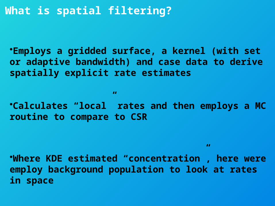
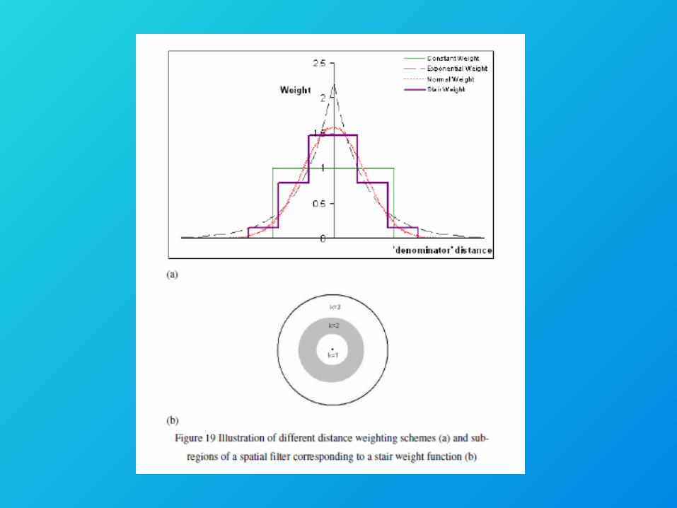
What is spatial filtering?

•Employs a gridded surface, a kernel (with set or adaptive bandwidth) and case data to derive spatially explicit rate estimates

•Calculates “local” rates and then employs a MC routine to compare to CSR

•Where KDE estimated “concentration”, here were employ background population to look at rates in space

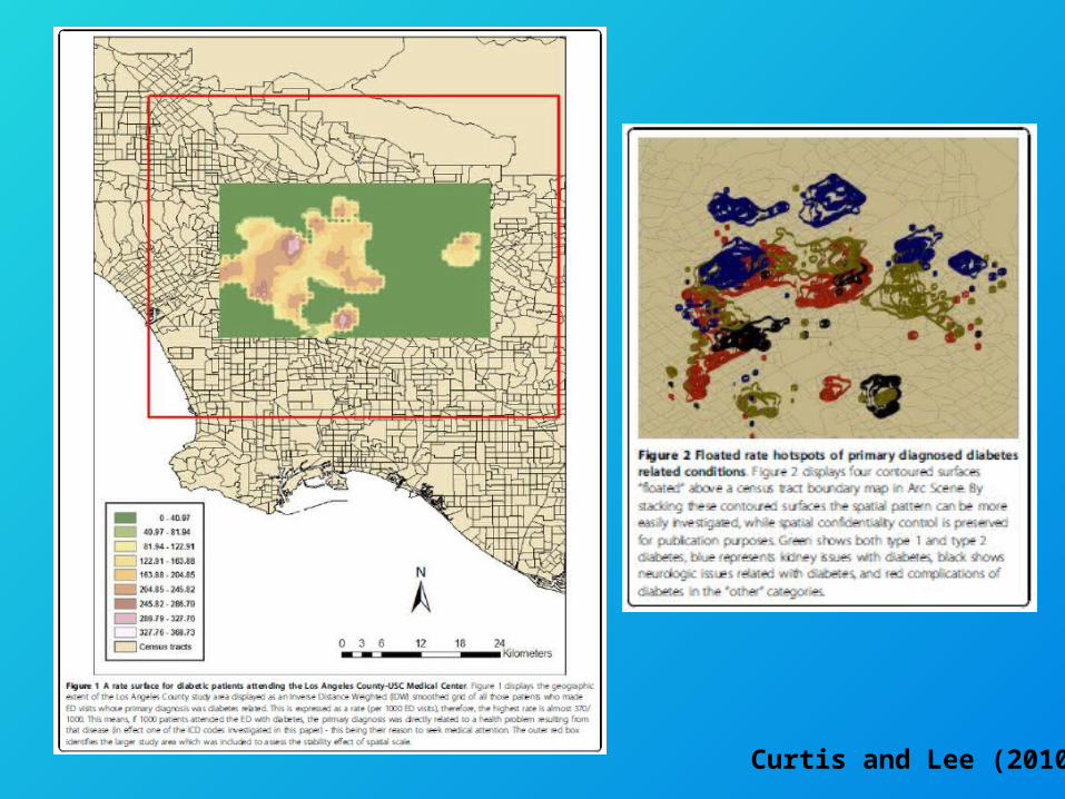
Curtis and Lee (2010)

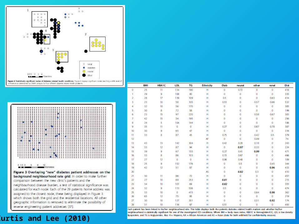
Curtis and Lee (2010)

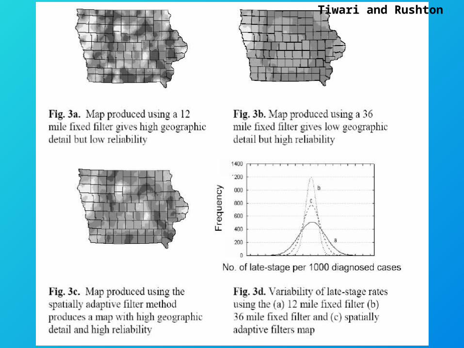
Tiwari and Rushton

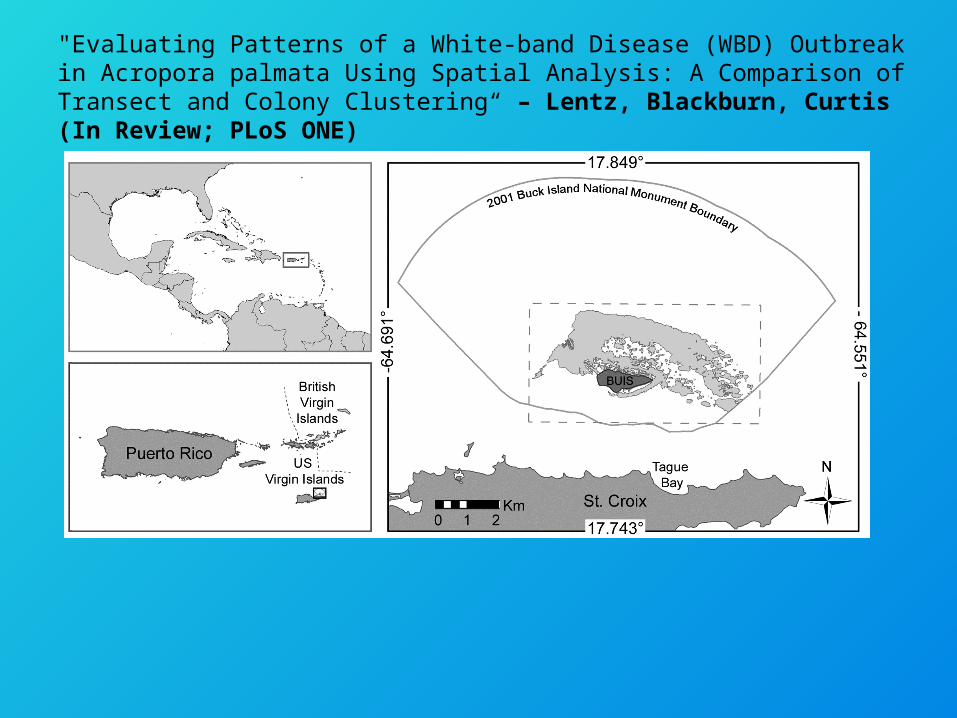
"Evaluating Patterns of a White-band Disease (WBD) Outbreak in Acropora palmata Using Spatial Analysis: A Comparison of Transect and Colony Clustering“ – Lentz, Blackburn, Curtis (In Review; PLoS ONE)

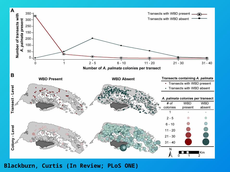
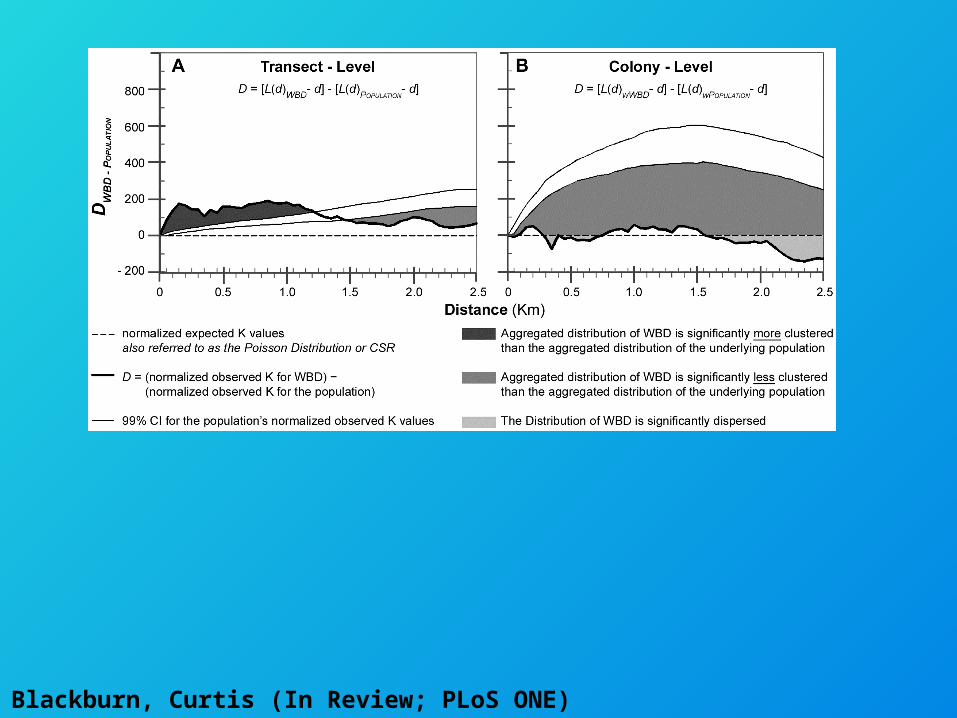
Lentz, Blackburn, Curtis (In Review; PLoS ONE)

Lentz, Blackburn, Curtis (In Review; PLoS ONE)

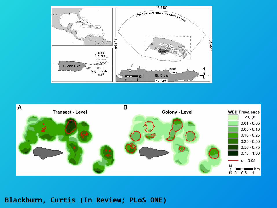
Lentz, Blackburn, Curtis (In Review; PLoS ONE)

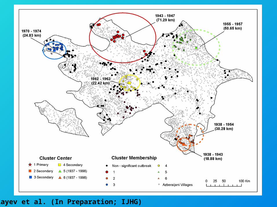
Abdullayev et al. (In Preparation; IJHG)

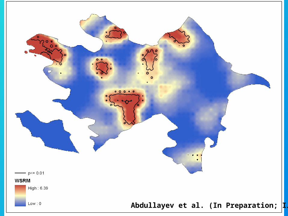
Abdullayev et al. (In Preparation; IJHG)

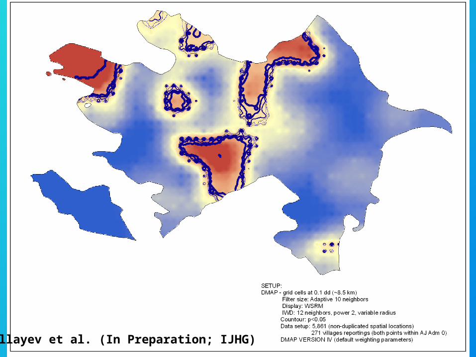
Abdullayev et al. (In Preparation; IJHG)

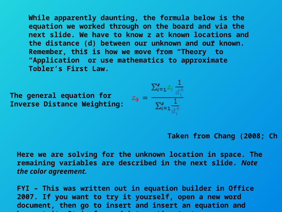
Here we are solving for the unknown location in space. The remaining variables are described in the next slide. Note the color agreement.

FYI – This was written out in equation builder in Office 2007. If you want to try it yourself, open a new word document, then go to insert and insert an equation and have at it. It is fun and interesting to try.

While apparently daunting, the formula below is the equation we worked through on the board and via the next slide. We have to know z at known locations and the distance (d) between our unknown and our known. Remember, this is how we move from “Theory” to “Application” or use mathematics to approximate Tobler’s First Law.

The general equation for Inverse Distance Weighting:

Taken from Chang (2008; Ch 16)

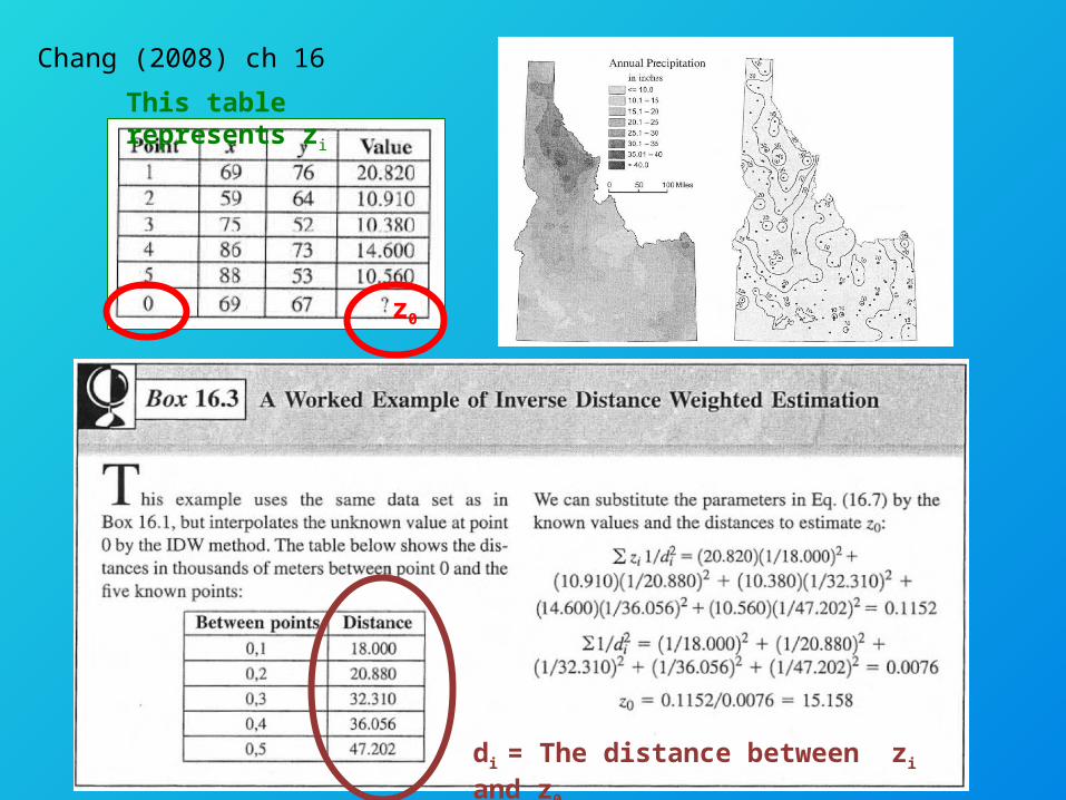
Chang (2008) ch 16

This table represents zi

z0

di = The distance between zi and z0