Embed Size (px)
Citation preview

Spatial distribution of vegetation in deserts: quantification and impact on aeolian geomorphology
Ian Oliver McGlynn Portsmouth, Virginia
B.S., George Washington University, 2003
A Thesis presented to the Graduate Faculty of the University of Virginia in Candidacy for the Degree of
Master of Science
Department of Environmental Sciences
University of Virginia May, 2006

ii
Notes Page Suggested Page Order:
1. Signed and Approved Title Page 2. Copyright page 3. Abstract (350 words) or Introduction 4. Table of Contents 5. Body of Text
(http://artsandsciences.virginia.edu/grad/degree/physical_standards.php ) (http://www.copyright.gov/register/literary.html)
© Copyright by Ian O. McGlynn
All Rights Reserved May 2006

iii
Abstract
Mineral dust aerosols suspended in the atmosphere impact atmospheric radiative
transfer, global and oceanic nutrient cycling, cloud formation and precipitation. The
entrainment of dust in desert environments is highly sensitive to vegetation cover that can
reduce erodibility and stabilize surfaces. It is essential to understand the relationship of
geospatial patterns of vegetation with arid geomorphology to refine the projection of dust
emissions in global climate change models. This thesis seeks to understand and estimate
the impacts of dust emission and transport from the spatial characterization of surface
roughness elements.
Arid and semi-arid region land degradation, or desertification, is fundamentally
linked to aeolian transport of mineral dust and encroachment and degradation of
vegetation. The spatial distribution of surface roughness elements such as vegetation or
large rocks may control wind erosion rate and dust emissions and, as a result, arid-region
geomorphology. Surface geomorphology is assumed to change from the hypothesis:
“dust emissions in the atmosphere are significantly increased by the encroachment of
shrubland through changes in the spatial distribution of vegetation, thereby degrading
arid deserts”. This hypothesis will be tested by two studies: (1) analysis of the pattern of
shrub infestation in degraded, aeolian dominated environments, and from (2) the
contribution of nonerodible roughness elements distribution in mineral dust flux
emissions.
A new geostatistical method presented in Chapter 2 provides a measure of the
spatial distribution of vegetation elements in a highly-degraded landscape. In the Jornada
del Muerto Basin in New Mexico, shrub encroachment is clearly evident from decreased

iv
intershrub patch size in coppice dunes of 27.8 m relative to shrublands of 65.2 m and
grassland spacing of 118.9 m, and a strong SW-NE duneland orientation correlates with
the prevailing wind direction and suggests a strong aeolian control of surface
geomorphology. In Chapter 3, a new model of aeolian flux incorporating the spatial
distribution of vegetation is presented. Shear stress inhomogeneity (m) for vegetated
surfaces, was found to have a non-linear relationship with gap size, was reduced with low
and high lateral cover (0.1<λ<0.3) and suggests possible wake interference at moderate
densities of λ=0.1

v
CONTENTS Abstract .............................................................................................................................. iii
Contents .............................................................................................................................. v
List of figures.................................................................................................................... vii
Acknowledgements............................................................................................................ ix
Chapter 1: Principles of aeolian erosion and geomorphology in deserts............................ 1
1. Introduction............................................................................................................. 1
2. Dust sources and global importance of dust ........................................................... 3
3. Aeolian processes related to production of mineral aerosols................................ 10
4. Effect of vegetation on dust emissions ................................................................. 15
5. Integration of remote sensing analyses ................................................................. 16
6. Structure of the thesis............................................................................................ 18
Chapter 2: Characterization of shrub distribution using high spatial resolution remote
sensing: Ecosystem implications for a former Chihuahuan Desert grassland .................. 20
1. Introduction........................................................................................................... 21
2. Material and experimental methods...................................................................... 24
3. Results................................................................................................................... 37
4. Discussion............................................................................................................. 43
5. Conclusion ............................................................................................................ 49
Chapter 3: Influence of vegetation spacing on wind erosion............................................ 51
1. Introduction........................................................................................................... 52
2. Methods................................................................................................................. 58
3. Results................................................................................................................... 65

vi
4. Discussion and Conclusions ................................................................................. 72
Cited References ............................................................................................................... 77

vii
List of figures Chapter 1: Principles of aeolian erosion and geomorphology in deserts............................ 1
Figure 1. Global distribution of arid environments ...................................................... 1
Figure 2. Comparison mean monthly temperature and precipitation of deserts ........... 2
Figure 3. Intercontinental aeolian transport of nutrients............................................... 6
Figure 4. Global distribution of dust emissions ............................................................ 9
Figure 5. Threshold friction velocity for a variety of particle diameters.................... 13
Chapter 2: Characterization of shrub distribution using high spatial resolution remote
sensing: Ecosystem implications for a former Chihuahuan Desert grassland .................. 20
Figure 1. Connectivity calculation.............................................................................. 25
Figure 2. Theoretical connectivity decay curve.......................................................... 26
Figure 3. Elongation from surface connectivity ......................................................... 27
Figure 4. Simulated images of different orientations used for testing connectivity
orientation angle........................................................................................... 28
Figure 5. Simulated images of different cover and range used for testing connectivity
orientation angle........................................................................................... 30
Figure 6. Jornada Experimental Range (JER), NM .................................................... 31
Figure 7. Aerial coverage and vegetation distribution, JER ....................................... 32
Figure 8. Object-oriented image classification ........................................................... 35
Figure 9. Connectivity orientation validation ............................................................. 38
Figure 10. Connectivity range validation.................................................................... 40
Figure 11. Orientation distribution for grasslands and coppice dunes........................ 42

viii
Chapter 3: Influence of vegetation spacing on wind erosion............................................ 51
Figure 1. Ratio of surface shear velocity to shear velocity for distance downwind of
fences ........................................................................................................... 56
Figure 2. Lateral profile similarity for roughness elements of different heights ........ 57
Figure 3. Average streamwise width versus lateral cover .......................................... 61
Figure 4. Wake development from surface roughness elements ................................ 62
Figure 5. Dust flux versus mean gap size from two field observations, JER, NM..... 64
Figure 6. Flux events for lateral cover from Owens Lake, CA................................... 65
Figure 7. Gap spacing at range distances for three gap distributions ......................... 68
Figure 8. Probability of total dust emissions for three gap distributions .................... 69
Figure 9. Comparison of dust emission models and field observations ..................... 71
Figure 10. Modeled dust flux from the Poisson distribution closely matches observed
field emissions ............................................................................................. 72
Figure 11. Shear stress inhomogeneity from low moderate and high densities of
vegetation..................................................................................................... 75

ix
Acknowledgements
Funding to support the research and analysis included in the thesis was supported
in part by the National Science Foundation grant DEB 03-16320.
My thesis advisor, Professor Gregory Okin has been a consistent source of
inspiration, professional guidance and technical support. His countless hours of teaching
guided this research through many challenges. This thesis would not have been
completed without his invaluable support. Special thanks towards committee members,
Professors Paolo D’Odorico and Hank Shugart for sharing their diverse expertise and
insights, and have been incredibly encouraging throughout all of my academic studies.
Additional thanks to my family and friends, who have tolerated and supported my
endeavors, academic and otherwise.

1
CHAPTER 1
Principles of aeolian erosion and geomorphology in deserts 1. INTRODUCTION
Continentality, anticyclonic subsidence, orographic influences, coastal upwelling
of cold water, and the highly reflective albedo of desert surfaces create the major
subtropical arid deserts, the majority of which are located between the equator to 30° N,
and on the western edge of continents (fig. 1).
Figure 1. One third of the Earth’s land surface is classified as semi-arid to hyper-arid, with deserts formed from anticyclone Hadley-Ferrel cell convergence at 30° N and S latitude, rain shadowing from orographic relief, and distance to moisture (from Houghton et al., 2001).
The deserts of the world are often considered to be barren wastelands incapable of
supporting life. They are associated with images of landscapes consisting of extensive
sand dunes, dry lakebeds, and limited vegetation. Deserts are highly varied landscapes
with robust vegetation and climatic conditions ranging from subhumid to hyperarid.
Drylands are found on every continent and cover nearly one-third of the Earth’s land
surface. Deserts may be defined in various ways, with climate, geomorphology, soils, and
2
vegetation considered in several definitions (Dregne and Chou, 1992). Generally
speaking, though, deserts are defined by a lack of water, which can be measured with
indices of aridity, developed as the moisture differential between inputs from
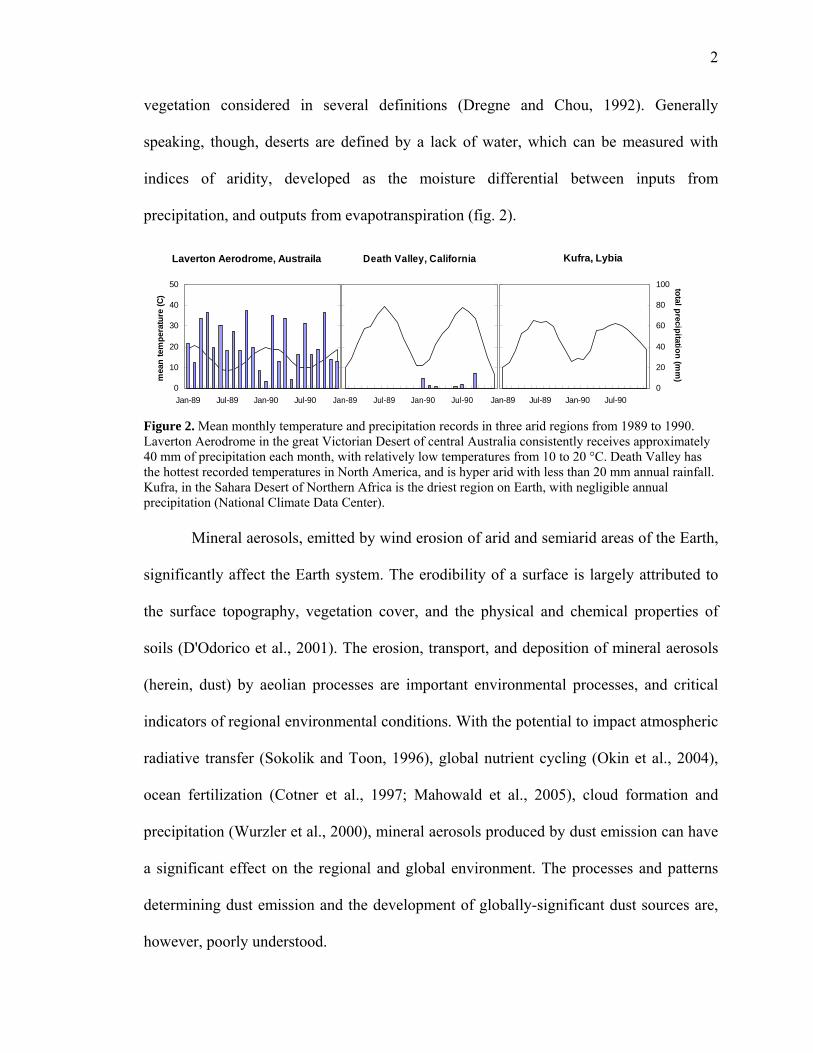
precipitation, and outputs from evapotranspiration (fig. 2).
Figure 2. Mean monthly temperature and precipitation records in three arid regions from 1989 to 1990. Laverton Aerodrome in the great Victorian Desert of central Australia consistently receives approximately 40 mm of precipitation each month, with relatively low temperatures from 10 to 20 °C. Death Valley has the hottest recorded temperatures in North America, and is hyper arid with less than 20 mm annual rainfall. Kufra, in the Sahara Desert of Northern Africa is the driest region on Earth, with negligible annual precipitation (National Climate Data Center).
Mineral aerosols, emitted by wind erosion of arid and semiarid areas of the Earth,
significantly affect the Earth system. The erodibility of a surface is largely attributed to
the surface topography, vegetation cover, and the physical and chemical properties of
soils (D'Odorico et al., 2001). The erosion, transport, and deposition of mineral aerosols
(herein, dust) by aeolian processes are important environmental processes, and critical
indicators of regional environmental conditions. With the potential to impact atmospheric
radiative transfer (Sokolik and Toon, 1996), global nutrient cycling (Okin et al., 2004),
ocean fertilization (Cotner et al., 1997; Mahowald et al., 2005), cloud formation and
precipitation (Wurzler et al., 2000), mineral aerosols produced by dust emission can have
a significant effect on the regional and global environment. The processes and patterns
determining dust emission and the development of globally-significant dust sources are,
however, poorly understood.
Laverton Aerodrome, Austraila
0
10
20
30
40
50
Jan-89 Jul-89 Jan-90 Jul-90
mea
n te
mpe
ratu
re (C
)
Death Valley, California
Jan-89 Jul-89 Jan-90 Jul-90
Kufra, Lybia
Jan-89 Jul-89 Jan-90 Jul-900
20
40
60
80
100 total precipitation (mm
)

3
2. DUST SOURCES AND GLOBAL IMPORTANCE OF DUST
Deserts are the primary source of mineral aerosols but there are a variety of
additional natural sources of aerosols in the atmosphere such as volcanic ejecta, smoke,
and sea salt (table 1). Anthropogenic aerosol sources include biomass burning and
industrial air pollution (Miller et al., 2004). This thesis will focus on mineral aerosols
produced by dust emission from deserts.
2.1. Nutrient cycling
The global biosphere is intricately linked through the chemical weathering,
transport and deposition of nutrients. Elements weathered from exposed geologic sources,
such as Mg, P, K, and Ca are essential for life. Regions with old, highly weathered soils
in humid climates such as oxisols in the Brazilian and Hawaiian rainforest or ultisols and
vertisols in Southeast Asia are depleted in mineral-derived nutrients, primarily
phosphorus-containing minerals. Although these regions are typically characterized as
having high nutrient retention, loss from leaching, fire, and erosion does occur. The loss
of mineral derived, biologically available nutrients necessitates foreign inputs to sustain
photosynthetic productivity. Mass-balance measurements of nutrient budgets,
atmospheric deposition, and isotope analysis of soils have shown that deposition of wind
transported nutrients can sustain regions at very large distances from the dust sources
(Chadwick et al., 1999). The geographically isolation region of Hawaii supports diverse
ecosystems and high productivity due, in part, to the influx of Mg, P, K, and Ca from
Asian sources over 6,000 miles to the west. Dust from North African deserts has been
attributed as the primary source of P for the P-limited Amazon Basin (Okin et al., 2004;

4
Swap et al., 1992). The disruption of mineral dust emissions and transport pathways can
lead to a systematic degradation of mineral-limited regions globally.
Table 1. Relative estimated contribution of mineral dust to total aerosol emissions (Tg/yr) in 2000 (from Houghton et al., 2001).
Northern Hemisphere
Southern Hemisphere Global Low High
Carbonaceous aerosols Organic matter (0-2 mm)
Biomass burning 28 26 54 45 80 Fossil fuel 28 0.4 28 10 30 Biogenic (>1 mm) -- -- 56 0 90
Black Carbon (0-2 mm) Biomass burning 2.9 2.7 5.7 5 9 Fossil fuel 6.5 0.1 6.6 6 8 Aircraft 0.005 0.0004 0.006
Industrial Dust (>1 mm) 100 40 130 Sea Salt
D<1 mm) 23 31 54 18 100 D=1-16 mm) 1420 1870 3290 1000 6000 Total 1440 1900 3340 1000 6000
Mineral Dust D<1 mm) 90 17 110 -- -- D=1-2 mm) 240 50 290 -- -- D=2-20 mm) 1470 282 1750 -- -- Total 1800 349 2150 1000 3000
Aeolian dust deposits are also a significant source of mineral-derived nutrients in
ocean environments. Large amounts of terrestrial-sourced dust particles are deposited in
the oceans (fig. 3). Wind-transported Fe, N, and P inputs are common, but only Fe and P
are readily soluble and easily accessible by microorganisms (Baker et al., 2006). Several
studies have suggested a restriction of microbial activity from phosphorous limitations in
the Atlantic and Indian oceans (Cotner et al., 1997; Sanudo-Wilhelmy et al., 2001), and
strong response of microbial biomass increase to iron sediments from large dust events in
the Pacific (Bishop et al., 2002; Mahowald et al., 2005).
2.2. Radiative transfer Incoming solar radiation drives the climate and most life on the planet. Aerosols
in the atmosphere can scatter and absorb solar radiation (Li et al., 1996), and have both
direct and indirect effects on climate. Direct effects result from the scattering or

5
absorption of radiation by aerosols in the atmosphere (fig. 4). Indirect effects result from
the impact of aerosols on cloud-forming processes, resulting in changes in cloud cover
that impact the radiation budget.
The direct effect of desert dust on global or regional climate is complex, because
dust can either scatter incoming short-wave solar radiation back to space or absorb
infrared light. Thus, the presence of dust in the atmosphere can result in a net negative or
net positive radiative forcing (Sokolik and Toon, 1996; Tegen et al., 1997). Negative
forcing due to increases in atmospheric albedo from the presence of scattering aerosols is
expected to be strongest over low-albedo regions such as oceans. Positive forcing, due to
absorption of incoming shortwave or outgoing longwave radiation is typical in desert
environments and other high-albedo surfaces such as snow, providing a strong thermal
contrast between continents and oceans. The presence of mineral dust has been shown to
reduce photolysis rates throughout the atmosphere (Liao et al., 1999).

6
Figure 3. Large-scale transport of and deposition from Saharan and central-Asian sourced P as mineral dust provides a substantial influx to highly depleted P regions in the Amazon basin, central Africa, and southeast Asia (from Okin et al., 2004).
African dust has been observed to be the predominant light-scattering aerosol
over the North Atlantic (Li et al., 1996). With a global climate model, Tegen et al. (1996)
suggested mineral aerosols create a negative global mean forcing at the surface of 1 W m-
2. More recent studies of direct radiative forcing have suggested a larger global decrease
of 1.9 W m-2 (Bellouin et al., 2005), and local radiative transfer models predicting 4.7 W
m-2 (Liao and Seinfeld, 1998).
In the presence of a cloud layer, radiative forcing by mineral aerosols is sensitive
to altitude (Haywood and Boucher, 2000). When atmospheric dust is above a cloud layer,
incoming solar radiation and reflected radiation from the clouds are absorbed, warming
the upper atmosphere from 3.5 to 5.0 W m-2 over low to high albedo surfaces, and

7
negative forcing of -1.5 to -0.8 W m-2. Dust below a cloud layer increases multiple
scattering with a lower radiative forcing in the upper atmosphere -0.2 to 2.0 W m-2 and
higher negative forcing on the surface -1.6 to -1.4 W m-2 (Liao and Seinfeld, 1998).
The indirect effects of mineral aserosols on atmospheric radiative transfer are not
yet fully understood. Clouds are the most important, and most variable, controls on total
planetary albedo. Mineral aerosols impact cloud formation because dust particles can
behave as cloud condensation nuclei (CCN) (Warner and Twomey, 1967). Thus, the
presence of dust can increase cloud cover, and hence albedo, while reducing precipitation
(Rosenfeld et al., 2001; Warner and Twomey, 1967). Suppression of precipitation has
been suggested to occur as the result in decreases in cloud droplet size related to
increases in CCN concentration. When atmospheric dust is above a cloud layer, incoming
solar radiation and reflected radiation from the clouds are absorbed, warming the upper
atmosphere from 3.5 to 5.0 W m-2 over low to high albedo surfaces, and negative forcing
of -1.5 to -0.8 W m-2. Dust below a cloud layer increases multiple scattering with a lower
radiative forcing in the upper atmosphere -0.2 to 2.0 W m-2 and higher negative forcing
on the surface -1.6 to -1.4 W m-2 (Liao and Seinfeld, 1998).
The intricate feedback of both positive and negative radiative forcing and high
uncertainty of predictions of future dust emissions hinders definitive assessment of how
mineral aerosols impact atmospheric radiative transfer. Preliminary estimates from the
Intergovernmental Panel on Climate Change (IPCC) science report predicted a net global
increase of dust emissions by 10% in 2100, but with high regional and spatial variability
(Houghton et al., 2001). Saharan dust refractive index measurements were inferred to
estimate a small net increase in radiative forcing globally. Up to 50% of mineral dust

8
emissions were attributed to anthropogenic land use changes. Past natural dust emissions
were assumed to be constant. Both assumptions are highly speculative and omit natural
variations in vegetation, climate, and atmospheric circulation which certainly have not
remained constant, and should contribute to high variability in dust emissions, as has
been reported for the past century (Prospero and Lamb, 2003). Accurate quantification of
dust sources and predictions of future spatial and temporal variability of emissions is
essential for substantial progress in climate change models.

9
Figure 4. Global distribution of dust emissions, concentrated in Northern Africa and Central Asia (A), corresponding with dust transport concentrated in Western Africa (B) (from Houghton et al., 2001).
(B)
(A)

10
3. AEOLIAN PROCESSES RELATED TO PRODUCTION OF MINERAL
AEROSOLS
The largest dust sources in the world are in hyperarid areas and drylakes. Dust
emissions can also originate from semiarid areas, particularly when the vegetation is
degraded or the surface is disturbed by anthropogenic activities. Desert dust generally
consists of sediment and soil particles with diameters from ~ 2 to 50 μm (Pye, 1987),
although only the smallest particles (< 10 μm) are transported long distances. Particles
are transported by wind through saltation, creep and suspension.
3.1. Law of the wall and friction velocity
Many attempts have been made to model desert dust emissions. Dust emission
models have been generally based on the observation that wind erosion and dust emission
are initiated when a minimum wind velocity threshold has been reached, and are not
linearly dependent upon wind velocity (Bagnold, 1941). At distances approaching a
surface, viscous flow dominates, creating a boundary layer with no pressure gradient. The
velocity profile near that surface approaches zero. Particle flux near the surface is
controlled not by the wind velocity, but by the roughness characteristics of the surface,
and the associated boundary layer thickness. Movement at the surface is characterized by
a relationship of shear stress ( 0τ ) and air density ( ρ ), known as friction velocity ( *u ).
0
*u τρ
≡ (1)
This can also be expressed with the law of the wall, where velocity and friction velocity
are a function and where *yuv
, y is a nondimensionalized distance.

11
*
*
( )yuU f f yu v
⎛ ⎞= =⎜ ⎟⎝ ⎠
(2)
For rough, natural surfaces, roughness elements must be introduced which disturb the
movement between the viscous sublayer and outer layer. The geometry of rough elements
on the surface create a pressure drag and modify the law of the wall to account for
roughness height, 0y and the von Karman constant ( k ) in turbulent flow.
* 0
1 lnU yu k y
⎛ ⎞= ⎜ ⎟
⎝ ⎠ (3)
In high density vegetated surfaces, the boundary profile becomes distorted near the
surface, which can be corrected as the difference between the height y and with the
introduction of mean momentum displacement d.
* 0
1 lnU y du k y
⎛ ⎞−= ⎜ ⎟
⎝ ⎠ (4)
A series of papers by Raupach (Raupach, 1991; Raupach, 1992; Raupach, 1994; Raupach
et al., 1993) presented a modification of roughness characteristics on saltating surface to
increase the roughness length. In areas of little or sparse vegetation, the roughness
sublayer below the mean momentum sink can be difficult to quantify but creates critical
sheltered areas from downwind wake effects which limit the predictive erodibilty of some
surfaces.
3.2. Wind threshold friction velocity
Several equations to predict horizontal aeolian flux have been suggested. One
such model is (Gillette et al., 1996):
2 2* * *( ) ( ) ( )tq x f x A u u u
gρ
= − (5)

12
where, q is the horizontal sediment flux (g/m s-1), A is a dimensionless constant, ρ is
the density of air, g is gravitational acceleration, *u is friction velocity, *tu is threshold
friction velocity. Once a particle movement has been initiated by overcoming the
threshold friction velocity, it often looses velocity and impacts into the surface. This
collision initiates the movement of disrupted surface particles from the impact, increasing
horizontal flux and creating an avalanche effect, similar to the propagation of downslope
snow movement. The saltation movement of particles along the surface increases the
aerodynamic roughness height. An internal boundary layer is formed from the increase in
surface roughness, creating a positive feedback system where both flux and roughness
can increase.
3.3. Sandblasting
Particle movement from saltation and sandblasting are the primary mechanism of
dust entrainment. Through the net horizontal movement of saltation, surface particles are
entrained by aerodynamic forces through a series of ballistic jumps on a centimeter scale
within the near-surface turbulent layer. Through sandblasting, particles can be entrained
at u* lower than soil saltation thresholds, transporting large particles and dust (Alfaro and
Gomes, 2001; Gomes et al., 1990). With each ballistic impact, kinetic energy and
momentum is transferred from impacting particles, and can break cohesive interparticle
bonds on the surface, releasing tightly-bonded, fine-grained desert dust (Shao et al.,
1993).
3.4. Grain size
The initiation of aeolian transport can occur at the minimum friction velocity, the
threshold friction velocity ( * *tu u= ). This initiation is when such as those due to

13
mineralogy, soil moisture, and microbial crusts, are less than the driving forces of
aerodynamic drag ( dF ) and lift ( lF ). For dry and bare surfaces, typical of arid and semi-
arid regions, Shao and Lu (2000 suggest a threshold equation modified from Greeley and
Iversen (1985), where NA is an experimental value for *tu and particle diameter derived
*t N pu A gd
dγσ
ρ⎛ ⎞
= +⎜ ⎟⎝ ⎠
(6)
from the particle friction Reynolds number where NA ~ 0.11-0.12 for d >200 μm, pσ is
the particle to air density ratio, d is particle size, and γ results from a curve fit. Wind
tunnel results give recommended values of 0.0123NA = , 4 23 10 kg sγ − −= × , assuming
spherical particles. Threshold friction velocity for a variety of diameters were shown by
Marticorena and Bergametti (1995) in figure 5.
Figure 5. Threshold friction velocity for a variety of particle diameters (from Marticorena and Bergametti 1995).
Physical characteristics such as the size distribution of loose particles and
atmospheric characteristics such as surface roughness are primary factors controlling the

14
aeolian erosion of surfaces. Bagnold (1941) and Marticorena and Bergametti (1995)
investigated the erosion threshold and erosion strength with surface roughness and wind
friction velocity.
( ) -1 -1* *, g cm stq f u u= (7)
While soil moisture and organic matter is not included, application of the model
determined emission production rates for a variety of soil ranges and surface types. Soil
size distribution, roughness length, and wind friction velocity were all considered to be
primary parameters. Analytical values for the various mechanisms acting upon soil
erosion previously mentioned were calculated. Suspension was found to act on particles
of sizes < 60 μm. Saltation occurs for particles from 60-2000 μm, where initiation of
movement can occur, but lift is insufficient to sustain transport. Larger particles (> 2000
μm) become too heavy for vertical movement and instead move along the surface, a
phenomenon known as creeping.
3.5. Soil moisture
Moist or wet soils have long been observed to experience little or no entrainment
of dust particles, relative to comparable dry surfaces, even when wind threshold
velocities are exceeded. Soil moisture creates interparticle bonds between surface grains
reducing the erosive potential. Capillary bonds in equilibrium with the atmosphere, create
a pressure differential between pore water particles and the air (Cornelis and Gabriels,
2003). Individual particles are also coated with a moist microlayer formed from a
polarized bond between charged particles called the electrostatic force (Ravi et al., in
press). Water may also act as an absorptive buffer, diminishing the momentum and
kinetic energy transfer to surface particles during bombardment. These cohesive forces

15
are likely to be in a constant state of disequilibrium, due to natural variability in surface
soil moisture via ambient humidity (Ravi and D'Odorico, 2005; Ravi et al., 2004).
4. EFFECT OF VEGETATION ON DUST EMISSIONS
The structure and spatial arrangement of vegetation modulates aeolian emission
and transport, and thus plays a pivotal relationship in controlling arid-region
geomorphology. Vegetation can have a strong influence on wind erosion rates and wind
erosion thresholds. While vegetation is associated with surface roughness, zero plane
displacement and boundary layer turbulence, the placement and distribution of vegetation
calls for increased scrutiny (Poggi et al., 2004). Vegetation present in arid regions resists
the erosion of soil, inhibits deflation, reduces surface velocity and provides sites for
deposition (Wolfe and Nickling, 1993).
As a driving factor of land degradation, soil erosion by wind is dependent upon
roughness properties of the surface. Threshold friction velocity ratio ( tR ), is the ratio of
the threshold friction velocity of erodible soil without roughness to that of a soil with
nonerodible roughness. Raupach et al. (1993) created a model for Rt, based on the
partitioning of shear stress between the vegetation and the soil surface:
1/ 2 1/ 2(1 ) (1 )tR m mσλ βλ− −= − + (8)where m <1 accounts for the stress difference from the substrate surface stress and the
maximum stress on the surface at a point, σ is the area ratio of the roughness element, λ
is the roughness density, and β is the ratio of the drag coefficient from a single, isolated
surface roughness element to the coefficient of drag for the substrate surface.

16
The first term ( ) 1 21 mσλ −− is the increase in stress on erodible surfaces and
( ) 1 21 mβλ −+ represents the decrease in stress in the shadowed area created by
nonerodible elements. Defined in terms of threshold friction velocity for vegetated
surfaces gives:
( )( )* * 1 1tv tsu u m mσλ βλ= − + (9)where β = 100, m = 0.5 for erodible surfaces of bare soil, and m= 1.0 for highly stable
surfaces. Nonuniform surface stress only affects the second parameter under the
radical ( ) 1 21 mβλ −+ , where typically ( ) 1 21 mσλ −− is unaffected in low densities of
1λ << .
5. INTEGRATION OF REMOTE SENSING ANALYSES
Remote sensing data products provide direct information on surface features and
offer a range of scales from which to view synoptic features. Remote sensing also affords
the best opportunity to study aeolian transport processes and geomorphology in harsh
conditions, assess environmental change over long periods, and on large scales infeasible
through traditional field-based methods. Remote sensing is a powerful tool for observing
the Earth’s surface and atmosphere. Most remote sensing studies of dust have focused on
dust in the atmosphere. A second class of studies has monitored and analyzed surfaces
features related to dust emissions.
5.1. Direct detection of airborne dust
Suspended dust in the atmosphere can be directly measured by an increasing
range of multispectral, hyperspectral, and multiangle active and passive instruments
(King et al., 1999). Solar radiation, reflected from the Earth’s surface is scattered and

17
absorbed by atmospheric constituents allowing for reliable measurements of mineral dust
aerosols, in addition to biogenic and anthropogenic sources. Platforms such as the TOMS
(Total Ozone Mapping Spectrometer) instrument with dual-channel UV sensors are
ideally suited to extract abundance in the atmosphere (Diaz et al., 2001; Torres et al.,
2002). Other platforms enable estimates of aerosol concentrations calculated from the
atmospheric optical thickness, aerosol size distributions, and scattering albedo, which
have been integrated into processed multispectral products (Satheesh et al., 2006; Tanre
et al., 1997). Common multispectral instruments such as MODIS (Moderate-resolution
Imaging Spectroradiometer) and AVHRR (Advanced Very High-Resolution Radiometer)
have had some success measuring aerosol retrieval from observed radiance to optical
depth (Husar et al., 1997; Karyampudi et al., 1999; Sokolik and Toon, 1999) but make
several assumptions on scattering dispersion patterns by aerosol constituents. Multiangle
instruments provide specific enhancements to measure aerosols, not viable with
traditional nidar instruments. Indirect (non-nidar) viewing angles enhance aerosol signals
from longer atmospheric path lengths. Aerosols of different compositions can also be
extracted from surface reflectance by anisotropic scattering at different angles (Diner et
al., 1999; Kaufman et al., 2002). Unfortunately, difficulties in spectral extraction of
aerosols between highly-reflective continents, and dark oceans persist, regardless of
instruments and methods. Aerosols-associated atmospheric features such as cloud
development and formation, and radiative forcing are also feasible. Geomorphic evidence
of aeolian transport, including dune mobility (Bullard, 1997) and aeolian deposition (Farr
and Chadwick, 1996) have also been examined using remote sensing.
5.2. Indirect assessment of dust mobilization from land surfaces properties

18
Studies that have used remote sensing to characterize the surface features that
directly control wind erosion are much less common than remote sensing studies of dust
once it is already aloft. However, remote sensing can provide information about surface
features that are associated with wind erosion and dust emission. Vegetation for example,
can be characterized by vegetation indices (e.g., EVI, LAI, NDVI), spectral-mixture
analyses (Okin et al., 2001b; Rango et al., 2000), and LIDAR (Rango et al., 2000).
Predicting future dust emissions with climate changes requires more detailed
understanding of global dust emissions, transport, and loading from large-scale studies of
sites with varying landcover. Adaptive vegetation measures must be developed to achieve
more accurate land cover characterization. Current classifications often focus on pixel-
based vegetation indexes such as NDVI, which are optimized for moist temperate regions
and perform poorly in the highly reflective environment with low vegetation cover,
typical of arid regions (Baret and Guyot, 1991; Huete et al., 2002). A utilization of
multispectral, multitemporal, and multiplatform data can enhance classifications of
dryland regions that provide information about surface conditions directly related to
aeolian transport.
6. STRUCTURE OF THE THESIS
Arid and semi-arid region land degradation is fundamentally linked to aeolian
transport and vegetation. However, the highly variable nature of vegetation makes it
difficult to characterize the precise relationship between the two. The spatial distribution
of vegetation may be a fundamental component of dust emissions as nonreodible
roughness elements and the association with aeolian erosion and resource availability.

19
Two studies will examine spatial components of vegetation cover and associated dust
emissions from the perspective of aeolian geomorphology. Geostatistical calculations on
remotely sensed datasets will be applied to specifically examine two aspects of arid
geomorphology: 1) the pattern of shrub infestation in degraded, aeolian dominated
environments, and 2) the contribution of nonerodible roughness elements distribution in
mineral dust flux emissions. A new geostatistical method presented in Chapter 2 provides
a measure of the spatial distribution of vegetation elements in a highly-degraded
landscape. In Chapter 3, an analysis of roughness elements is performed to demonstrate
the importance of spatial relationships of vegetation with dust emissions. A new model of
aeolian flux incorporating the spatial distribution of vegetation is presented.

20
CHAPTER 2
Characterization of shrub distribution using high spatial resolution remote sensing: Ecosystem implications for a former Chihuahuan
Desert grassland
(This chapter is in Remote Sensing of Environment, 101 (2006) 554-566.)
Abstract
Patchiness is often considered a defining quality of ecosystems in arid and
semiarid regions. The spatial distribution of vegetation patches and soil nutrients coupled
with wind and water erosion as well as biotic processes are believed to have an influence
on land degradation. A geostatistical measure of spatial “connectivity” is presented to
directly measure the size of patches in the landscape from a raster dataset. Connectivity is
defined as the probability that adjacent pixels belong to the same type of patch.
Connectivity allows the size distribution of erodible patches to be quantified from a
remote sensing image or field measurement, or specified for the purposes of modeling.
Applied to high-resolution remote sensing imagery in the Jornada del Muerto
Basin in New Mexico, the spatial distribution of plants indicates the current state of
grassland-to-shrubland transition in addition to processes of degradation in this former
grassland. Shrub encroachment is clearly evident from decreased intershrub patch size in
coppice dunes of 27.8 m relative to shrublands of 65.2 m and grassland spacing of 118.9
m. Shrub patches remain a consistent 2-4 m diameter regardless of the development of
bush encroachment. A strong SW-NE duneland orientation correlates with the prevailing
wind direction and suggests a strong aeolian control of surface geomorphology.

21
With appropriate datasets and classification, potential applications of the
connectivity method extend beyond vegetation dynamics, including mineralogy mapping,
preserve planning, habitat fragmentation, pore spacing in surface hydrology, and
microbial community dynamics.
1. INTRODUCTION
Shrub encroachment is a global phenomenon documented in arid and semi-arid
regions of Africa, Australia, and North America (Archer, 1995; Fensham et al., 2005;
Roques et al., 2001). In the Chihuahuan Desert grasslands of North America, shrub
encroachment has been especially pronounced, with significant transformation of
vegetation community structure occurring in the last 150 years. Populations of grasses,
primarily black grama (Bouteloua eriopoda) once dominated 90% of the region but have
diminished to less than 25% (Buffington and Herbel, 1965; Gibbens et al., 2005).
Drought-resistant shrub cover, primarily comprised of creosote (Larrea tridentata) and
mesquite (Prosopis glandulosa), has increased by a factor of 10 over the same period,
replacing the native grasses (Gibbens et al., 2005; Rango et al., 2000; Reynolds et al.,
1999). Causes of shrub encroachment and grassland deterioration such as rainfall
variability, elevated CO2, changes in fire regime, seed dispersal and livestock grazing
have been suggested (Archer, 1995; Scanlon et al., 2005), but the definitive cause of the
transformation remains unknown (Archer, 1995; Bahre and Shelton, 1993; Dougill and
Thomas, 2004).

22
The change in the spatial distribution of vegetation is an important aspect of shrub
invasion. Shrubs create “islands of fertility” by trapping soil resources beneath their
canopies (Schlesinger et al., 1990; Whitford, 1992). The transition from grass to shrub
cover increases the scale of spatial heterogeneity and the dominant small-scale processes
can be reflected through the position of individual plants (Schlesinger and Pilmanis,
1998). Thus, the ability to quantify the spatial distribution of plants could indicate the
current state of transition in addition to processes of degradation in semiarid mixed-shrub
grasslands.
Remote sensing provides an opportunity to monitor and understand spatial
patterns of vegetation and to inform the understanding of biotic and abiotic processes
related to those patterns. The physical and spectral properties associated with vegetation
cover and surface morphologic structures observed by remote sensing are being
continuously refined (Bradley and Mustard, 2005; Okin and Painter, 2004; Okin et al.,
2001b; Weeks et al., 1996) especially with the incorporation of spatial patterns of
vegetation (Caylor et al., 2004; Okin and Gillette, 2001; Privette et al., 2004; Scholes et
al., 2004).
High spatial resolution remote sensing enables direct imaging of plant individuals
that are at least the size of the ground resolution of the remote sensing image. This
capability makes possible demographic studies of vegetation such as Schlesinger and
Gramenopoulos’s (1996) use of archival photographs to show that there were not climate-
induced changes in woody vegetation in the Sudan from 1943 to 1994, and with
individual-based monitoring of vegetation change in the Jornada Basin (Rango et al.,
2002).

23
The ability to image individual plants with high resolution remote sensing opens
up the possibility of effective use of geostatistical methods for describing the distribution
of plants. Phinn et al., (1996) and Okin and Gillette (2001) have shown that traditional
variograms can provide an accurate measure of average plant spacing in shrublands of the
Chihuahuan Desert. Nonetheless, variograms provide limited information about the
landscape. In particular, because variograms are calculated on the basis of pairs of data
separated by some distance (lag), this method cannot provide information about
conditions between these pairs. In landscapes where the connectedness of soil or
vegetation patches (providing conduits for wind, water, seeds, small mammals, etc.) is
important, a different geostatistical metric of two-dimensional landscape structure is
advisable.
A new application of geostatistical techniques is presented to evaluate the
connectivity of plant and soil patches. This connectivity function calculates the
probability that contiguous pixels belong to the same class, or in this application, the
probability that contiguous pixels are or are not occupied by shrubs.
In this study, we present the use of connectivity to provide spatial information about
patch size and anisotropy and show that the results are robust for patchy landscapes.
Using an object-oriented classification on digitized orthophotos of our field site in New
Mexico, individual 1 m pixels are separated into shrub and not-shrub classes. We then
apply the connectivity statistic to the classified images to characterize the spatial nature
of shrub encroachment and the spatial characterization of individual shrub patches. As a
geostatistical measure, the use of connectivity is independent of the choice of
classification scheme. The progressive nature of shrub encroachment is evaluated through

24
the comparison of shrub and intershrub patch characteristics amongst differing areas of
establishment. Specifically, we present the theory and definition of connectivity
geostatistics, provide validation of connectivity based on stochastic simulation, and
demonstrate the utility of connectivity using a case study to examine the variability of
spatial distribution of vegetation in the Jornada Basin of New Mexico.
2. MATERIAL AND EXPERIMENTAL METHODS
2.1. Connectivity
We used a geostatistical measure of the connectedness of patches in the landscape
called “connectivity.” For a raster dataset, connectivity is defined as:
∑ ∏ ⎟
⎟⎠
⎞⎜⎜⎝
⎛=
n hiI
nhC 1)( (1)
where C is the connectivity, h is the lag vector with length |h|, n is the number of
consecutive sets of pixels along h in an image, and Ii is an indicator variable equal to 1
for pixels that belong to the class of interest and 0 otherwise. The connectivity at h =0 is
denoted as Co and is equal to the fraction of pixels in an image that belong to the class of
interest. For example, if “shrub” is the class of interest, then pixels that are classified as
“shrub” are given a value of 1, and all other pixels are given a value of 0. In this case, Co
will be equal to the fraction of pixels that are classified as “shrub”, or in other words, the
fractional shrub cover.
Connectivity may also be interpreted as a probability. In the case of Co, the
connectivity is the probability that any pixel in an image belongs to the class of interest.
C( h ) is the probability that any set of consecutive pixels along h all belong to the class

25
of interest (fig. 1). When interpreted as probabilities, it is intuitive that connectivity
always decreases with increasing lag distance, |h|.
In practice, the decrease in connectivity with |h| approximates an exponential
decay function (fig. 2). Thus, to derive a single statistic for the spatial scale of landscape
connectedness similar to the “range” in traditional variograms, we modeled connectivity
as:
⎟⎟⎠
⎞⎜⎜⎝
⎛−=
α||exp)( hChC o
r
(2)
From Equation (2), it is clear that the range (α) is an e-folding distance at which the
connectivity drops to Co/e.
Figure 1. Connectivity is calculated on the number of consecutive sets of pixels in an image, as 1 for pixels that belong to the class of interest and 0 otherwise with increasing lag distance, as demonstrated for 1, 2, and 3 pixel distances.
Lag is treated as a vector h , allowing for connectivity to be calculated along any
azimuth in an image, and α can be determined as a function of azimuth angle. In this
study, the resulting polar plots of azimuth and range were smoothed using a low pass fast
Fourier transform filter. Geometric properties were derived from the curves such as
orientation, the preferential azimuth, and elongation (fig 3). Elongation is defined as:
0 0 0 0 0 0 1
0 0 0 1
0 1 1 0
0
C(2): = 1/7 = 0.143
C(1): = 3/8 = 0.375
C(0): = 6/9 = 0.667
1
1 1 1 0 1
1 0

26
max
max
elongation αα
=⊥
(3)
the ratio of the maximum range (αmax) and the range perpendicular to the maximum
azimuth, α ⊥αmax( ).
The integration of continuously similar or connected values has been presented in
broad applications of geospatial components. Investigations into water transport include
spatial connectivity of river channels (Krishnan and Journel, 2003) fractured rocks with
three-dimensional percolation from small- to large-scale fault networks(Bour and Davy,
1998), the spatial density of connectivity of fracture networks in rocks with interest in
water transport (Renshaw, 1999), and homogenous soil moisture patterns (Western et al.,
1998). Incorporation of our connectivity statistic may expand the usage of multiple-point
spatial distributions in hydrogeology and throughout the environmental sciences.
|h|
0 5 10 15
C
0.0
0.1
0.2
0.3connectivity decayrange estimation
α = 4.02
C = 0.20/e = 0.073
Figure 2. Representative connectivity curve for 20% cover, a range of 4.02 (dashed line) and generally approximates an exponential decay curve.

27
2.2. Connectivity simulations
To verify that connectivity provides a robust representation of spatial patterns in
remote sensing imagery, a series of tests were performed on simulated images created
using the geostatistical software package GSLib (Deutsch and Journel, 1998). The
simulated images were generated using the unconditional simulated annealing algorithm
with variogram constraints.
0
5
10
15
20
Selden Canyon
North
E
S
Lag
Dis
tanc
e (m
)
major axis
minor axis
α max=16.8
θ=28o
⊥ αm
ax =13.3
θ=118 o
Figure 3. Polar plot of elongation values (dotted line) smoothed with a Fast- Fourier Transform (FFT) (solid line) and dominant orientation direction from the major axis.
28
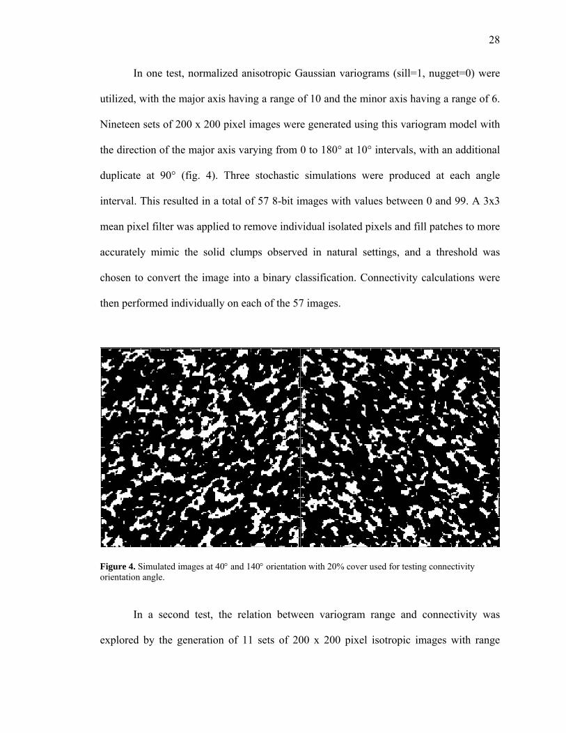
In one test, normalized anisotropic Gaussian variograms (sill=1, nugget=0) were
utilized, with the major axis having a range of 10 and the minor axis having a range of 6.
Nineteen sets of 200 x 200 pixel images were generated using this variogram model with
the direction of the major axis varying from 0 to 180° at 10° intervals, with an additional
duplicate at 90° (fig. 4). Three stochastic simulations were produced at each angle
interval. This resulted in a total of 57 8-bit images with values between 0 and 99. A 3x3
mean pixel filter was applied to remove individual isolated pixels and fill patches to more
accurately mimic the solid clumps observed in natural settings, and a threshold was
chosen to convert the image into a binary classification. Connectivity calculations were
then performed individually on each of the 57 images.
Figure 4. Simulated images at 40° and 140° orientation with 20% cover used for testing connectivity orientation angle.
In a second test, the relation between variogram range and connectivity was
explored by the generation of 11 sets of 200 x 200 pixel isotropic images with range

29
values from 1 to 20 pixels and one set at 40 pixels using the same variogram model (fig.
5). The simulated images provided a direct analysis of the dependence of connectivity on
patch size. A 3x3 mean pixel filter was then applied to the resulting 33 8-bit images with
values between 0 and 99. For each image the cumulative distribution function (CDF) was
calculated, allowing the creation of images with a specified fraction of each image below
a specific threshold determined from the CDF. These images mimic in appearance
orthophotos classified into shrub and not-shrub classes, with the scale of shrub patches
defined by the range of the variogram used to in the simulation. Connectivity range
calculations were performed on images with simulated cover varying from 10% to 90%
in 10% increments. The mean connectivity range of three realizations with each
variogram range and fractional cover are reported.

30
Figure 5. Simulated images at 0° orientation with 30% (top) and 70% (bottom) cover and a controlled range of 5 (left) and 10 (right) pixels. 2.3. Study area
The connectivity method provides a quantitative method to measure the
vegetation characteristics in different landscapes. Connectivity was tested on a series of
images from the Jornada Experimental Range (JER), located in the Chihuahuan Desert of
New Mexico, near the town of Las Cruces (fig. 6). This area has experienced dramatic

31
changes in vegetation cover from semiarid grasslands to arid shrubs. Detailed discussions
provided by Buffington and Herbel (1965) and Gibbens et al. (2005) describe the Jornada
transition from primarily native perennial grasses (Bouteloua spp.) to drought resistant
mesquite (Prosopis glandulosa) and creosote (Larrea spp.). This form of arid land
degradation has been attributed to climate change and intensive land use for pastoral
purposes.
Figure 6. Location of the Jornada Experimental Range (JER) in south-central New Mexico
This study focuses on the distribution of shrubs in the sand sheet area of the
Jornada Basin that comprises the western portion of the JER (fig. 7). The sand sheet
exists as a mosaic of patches ranging from mesquite coppice dunes with little to no grass

32
cover to grasslands with isolated mesquites. There are almost no areas in the JER sand
sheet that do not contain some mesquite.
Figure 7. Aerial coverage of digital orthophotos used in this study from October 1996 (striped) and land cover stratification (modified from Gibbens et al., 2005). 2.4. Classification of high-resolution aerial photography
The spatial distribution of vegetation can be ascertained from connectivity
calculations of high-resolution aerial photography, which must be first separated into a
binary classification of interest. Connectivity can only be calculated for images with a

33
binary representation of 1 for the class of interest and 0 for all other classes (equation 1).
The use of connectivity is independent of the choice of classification scheme. When
shrubs are defined as the class of interest, connectivity calculations provide information
about the size and shape of shrubs. When the non-shrub classes are defined as the class of
interest, connectivity provides information about the size and shape of intershrub patches.
An object-oriented supervised classification was performed on seven digital
orthophoto quarter quadrangle (DOQ) natural color aerial photos, originally flown by the
USGS in October 1996. One meter ground pixel resolution imagery provides sufficient
detail to derive relevant spatial information on mesquite shrubs found in the Jornada sand
sheet, as demonstrated by Phinn et al. (1996). Individual mesquite plants larger than 1 m
can be identified from the high-resolution imagery and therefore provide an opportunity
to examine and extract land cover through both spectral and spatial characteristics
through the differentiation of individual shrubs relative to the background of bare soil and
grass.
The use of an object-oriented analysis in this study provides many advantages
over traditional pixel-based classifications (Geneletti and Gorte, 2003). Object-oriented
classification groups adjacent pixels into contiguous multidimentionally homogenous
clusters that represent natural land cover patterns and minimize classification errors that
result from single pixels with outlier values and areas of complex spectra due to mixed
coverage. Thus, this classification procedure can account for the spatial relationship of
pixels, not just the spectral values. This method is gaining increasing acceptance as it
proliferates throughout the remote sensing community (Dorren et al., 2003) and has been
successfully used by Laliberte et al. (2004) at the JER.

34
For this study, pixels were identified as shrubs or non-shrub cover through a
series of segmentation and classifications in the eCognition software (fig. 8). The images
were divided into object segments according to size, shape and digital number value from
all three visible bands. The segmentation process subdivides the images into groups of
pixels based on scale-dependent homogeneity. Single pixels are gradually built-up into
larger clusters while accounting for high spectral homogeneity of shrubs relative to soil
and the size of shrubs. A maximum object heterogeneity or scale parameter of 6 was used
to constrain object sizes and a high emphasis on object compactness and shape to
maximize the distinction between shrubs, grasses, and soil. Scale parameter analysis
indicated 25% of neighborhoods had a value around 8.62 pixels. All three visible bands
had the same spectral weighting for segmentation. Baatz and Schape (2000) provide
further description of the segmentation procedure. Supervised classifications were
performed on segmented images using a nearest-neighbor approach from the training
classes of intensity values for shrub cover, grass cover and soils, and finally grouped
according to classes of interest.

35
Figure 8. Object-oriented classification process from A) digital orthophoto with darker areas represent shrub patches while the lighter background represents grasses and bare soil, B) image segmentation with irregular shapes representing pixels grouped by shape and similar intensity, C) supervised classification where segments are grouped into regions of shrub cover (dark), grasses and mixed vegetation (intermediate) and bare soil (light) D) extracted binary classification feature of shrub (dark) and no-shrub (light).
While features such as shrubs are easily identified and classified, several
limitations are inherent with the use of high spatial-resolution color imagery. Without the
availability of high spectral resolution data, it is not possible to accurately distinguish
amongst shrub types through a comparison of spectral reflectance. Additionally,
centimeter or decimeter-scale vegetation such as grasses cannot be directly detected from
meter-scale imagery.
C D
B A

36
2.5. Connectivity analysis of classified remote sensing imagery
The classified visible digital images were divided into 200 x 200 pixel subimages
in which connectivity was calculated, first with shrubs as the class of interest, then as the
non-shrub component as the class of interest. These calculations were performed for lag
distances from 0-40 m, at two-degree intervals from 0-360°. Range, elongation, and
orientation values for each subimage were then integrated into a new coregistered image
with 200 x 200 m pixels. When range, elongation, and orientation are calculated with
shrub as the class of interest, these statistics provide information about the size and shape
distribution of contiguous areas occupied by shrubs. When these statistics are calculated
with the not-shrub as the class of interest, they provide information about the size and
shape distribution of intershrub areas that may be comprised of bare soil, grasses, or a
mixture of bare soil and grasses.
2.6. Environmental stratification
The range, geometric elongation, and orientation data were stratified based on a
dominant vegetation land cover map, developed from field studies in 1998 (Gibbens et
al., 2005). The dominant land cover classification in each subimage was determined and
compared with calculated connectivity range, elongation, and orientation. Stratifying
orientation and elongation results based on vegetation cover allows for the comparison of
shrub distribution within regions of variable shrub infestation.

37
3. RESULTS
3.1. Connectivity analysis of simulated images
The connectivity method presented here can determine the direction of anisotropy
in simulated images. Figure 9 shows a strong 1:1 relationship between the orientation
angle calculated from connectivity and the major-axis of anisotropy used to generate the
simulated images (expected angle). The relationship between the range of isotropic
variograms used to generate simulated images and the connectivity range is shown in
Figure 10. The connectivity range increases with increasing variogram range, but flattens
out when variogram range reaches about 10 pixels. The connectivity range is also a
function of the fractional cover in simulated images, with lower cover resulting in lower
connectivity ranges, when connectivity is calculated on the basis of the cover class. When
connectivity is calculated on the basis of the non-cover class, lower cover results in
greater connectivity ranges (not shown). These results show that connectivity is able to
provide an indication of both the direction of anisotropy and an index of the patch size in
simulated images. The index of patch size provided by connectivity (e.g., the connectivity
range) is different from that provided by the variogram range used to produce the
simulated images. This is due to the fact that connectivity provides a fundamentally
different measure of spatial autocorrelation than variograms. Thus, connectivity can be
used to augment spatial information from traditional variography and can provide
important measures of patch size for categorical data.

38
y = 0.9957xR2 = 0.9909
0
30
60
90
120
150
180
0 30 60 90 120 150 180
expected orientation angle (°)
calc
ulat
ed o
rient
atio
n an
gle
(°)
Figure 9. Calculated orientation angle versus expected orientation angle for images created using the simulated annealing algorithm in GSLIB. Expected orientation angle is the angle of the major-axis of the variogram used to create each image. Calculated orientation angle is the angle of orientation determined by the connectivity method presented here. Each point is the mean for three realizations (generated images) at 20% cover.
3.2. Object-oriented classification
The use of 1 m orthophotos imagery provides a suitable resolution to detect the
presence of shrubs (Laliberte et al., 2004). Due to the size, grass clumps are difficult to
distinguish from the soil background, although further study may overcome this
limitation to separate shrubs, grass-covered soils, and bare soils at 1 m resolution. As a
result, classification of the orthophotos images with eCognition resulted in maps of the
presence or absence of mesquite shrubs, the dominant shrub in the sandsheet are of the

39
JER. Most of the area was classified as bare soil and grasses, while only 14% of pixel
area was classified as shrubs (table 1). Shade dominated pixels may have been
misclassified as shrubs in two of the seven images, although unlikely due to visual
inspection, spectral differentiation of land cover, the geometric profile of topographically
high shrubs, and relatively low leaf area index (LAI) typical of vegetation in October.
The maps of mesquite resulted in estimates of fractional cover consistent with other
reports (Laliberte et al., 2004; Okin and Gillette, 2001).
Table 1. Major-axis range corresponding to dominant vegetation cover.
maximum range (m) mean range (m) median range (m) std. dev. land cover class shrub intershrub shrub intershrub shrub intershrub shrub intershrub
% cover
Grasslands 36.0 327.0 3.5 118.9 2.5 101.3 3.4 83.4 5.2 Mesquite 83.1 325.0 3.1 65.2 2.2 39.7 3.8 69.9 13.4 Mesquite dunes 10.9 227.1 2.5 27.8 2.4 22.8 0.6 20.6 15.0
3.3. Shrub connectivity range, elongation, and orientation
Connectivity calculations performed on 200 x 200 m subimages using the shrub
class as the class of interest provide information on the size and shape of shrub patches.
Major-axis, minor-axis, and mean range values for the shrub class are significantly
smaller than those for the non-shrub class indicating that mesquite shrubs are generally
smaller than the spaces between them (table 1). Median shrub patch size (i.e., median
shrub range) does not vary significantly in size with location or the land cover
classification from Gibbens, et al. (2005), though the standard deviation of the range is
less for mesquite dunes than for either mesquite or grassland areas.

40
controlled variogram range (pixels)
5 10 15 20
mea
n co
nnec
tivity
rang
e (p
ixel
s)
0
2
4
6
8
10
12
1470%50%30%10%
Figure 10. Calculated range distances verses control range sizes for images created using the simulated annealing algorithm in GSLIB. Controlled range is the size of the x and y axes of the variogram used to create each image. Mean connectivity range is the range distance determined by the connectivity method presented here, calculated at 10, 30, 50, and 70% of image cover. Each point is the mean of the major and minor range values for three realizations.
Elongation values are constrained to ≥ 1.0, thus mean and median elongation
values are always > 1.0 (table 2). For analysis of elongation values, the ratio of the
standard deviation of elongation to the amount that the median value deviates from one
provides an index of the organization of the anisotropy akin to the coefficient of
variation:
Variability Index (VI) = Standard Deviation of Elongation/(Median of Elongation – 1) (4)
As the VI approaches 1, the anisotropy of shrub or intershrub patches becomes
increasingly consistent. Shrub patches tend to be the same size and shape and therefore
the VI for the shrub class in all cover types is close to 1.0. Shrub patches in mesquite

41
areas having the highest value VI = 1.3, which indicates a greater diversity of shrub
shapes in these areas.
Table 2. Elongation values for 200 m x 200 m subimages from different land cover classes. mean elongation median elongation std. dev. variability index land cover class
shrub intershrub shrub intershrub shrub intershrub shrub intershrub Grasslands 1.1 2.3 1.1 1.3 0.2 11.5 2.5 46.0 Mesquite 1.1 1.3 1.0 1.1 0.1 2.4 2.7 26.1 Mesquite dunes 1.1 1.1 1.1 1.1 0.1 0.1 1.3 1.2
In subimages dominated by mesquite dunes, the major-axis of anisotropy (e.g.,
the direction of the greatest range value) is oriented roughly northeast-southwest (fig. 11).
For mesquite dune subimages, orientation of shrub patches is clustered between 30° and
59° azimuth and orientation intershrub patches ranges from 0°-59°. In contrast, no clear
preferential orientation of shrub patches was detected for those subimages dominated by
grass or mixed grass-shrub vegetation.
3.4. Intershrub connectivity range, elongation, and orientation
Connectivity calculations using the non-shrub classes as the class of interest
provide information on the size and shape of intershrub areas. The mean range for
intershrub patch size varies significantly with landcover (table 1). Mean and median
distances are noticeably larger for areas of grasslands when compared to mesquite and
mesquite dunes. The range of intershrub patch size (e.g., the mean distance between
shrubs) decreases from 119 m in mixed vegetation to 65 m in mesquite, and 28 m in
mesquite coppice dunes. Median range decreases from 101 m in grass-dominated areas to
40 m in mesquite-dominated areas to 23 m in areas dominated by mesquite dunes. The
smaller intershrub distances in mesquite dunes indicate a higher density of shrubs in
regions of mesquite and mesquite dunes with respect to areas of grasses. Where shrub

42
grasslands n=560
0
0.2
0.4
0.6
0.8
0-29° 30-59° 60-89° 90-119° 120-149° 150-179°
frequ
ency
shrubintershrub
mesquite dunes n=2450
0
0.2
0.4
0.6
0.8
0-29° 30-59° 60-89° 90-119° 120-149° 150-179°
dominant orientation
frequ
ency
Figure 11. Histogram of orientation for shrub and intershrub patches for grasslands and mesquite which indicate no preferential orientation, and mesquite dunes showing strong preferential orientation.

43
size is nearly constant, intershrub distances are inversely related to plant density
reflecting an increasing continuum in shrub number density from grasslands to mesquite
dunes.
VI (equation 4) calculated from elongation values for intershrub patches in areas
dominated by grassland and mesquite all deviate significantly from 1.0 indicating a large
diversity in intershrub patch shape in these areas. In mesquite dunelands, VI = 1.3
indicates a consistent intershrub patch shape in these areas, with a slight elongation of
1.1. Values of VI > 1.3 for intershrub areas in non-dunelands is consistent with irregular
mesquite invasion in these areas and increasingly regular, but anisotropic, mesquite
establishment, as mesquite density increases until the VI = 1.2 in mesquite dunelands.
Orientations of intershrub patches clearly shows a variation between landcover
types, generally similar to the orientation differentiation of the shrub class of interests
(fig. 11). A lack of clear preferential orientation is present in grassland and mesquite
regions. The strong orientation found for shrubs in a general SW-NE orientation in
mesquite dunes cover is also present for intershrub areas in this landcover type.
4. DISCUSSION
Connectivity calculations performed on high resolution digital images provides
information on the size and shape of both shrubs and intershrub patches. Stratified by
dominant landcover types, variations in shrub and non-shrub distribution reflect the
progressive nature of the transition from grassland to shrubland, evident throughout the
JER (Gibbens et al., 2005; Laliberte et al., 2004).
44
Analysis of 1-m orthophotos also provides a direct measurement of the anisotropy
of mesquite distribution in the sandsheet portion of the JER. Dominant orientations
suggest that the presence of isotropic and anisotropic spatial distribution can be detected
using the method presented here. The strength of this anisotropy requires explanation and
clearly disputes the widely-used assumption of homogeneous (Gillette and Stockton,
1989; Musick and Gillette, 1990b) or random (Marticorena and Bergametti, 1995)
distributions of land cover in models.
The influences of spatial patterns of vegetation have significant implications for
aeolian emission and transport modeling of arid landscape degradation. Shrubs and
intershrub patches in areas of mesquite coppice dunes show a strong northeast-southwest
orientation, and agreeing with earlier studies by Okin and Gillette (2001) and Gillette and
Pitchford (2004) that suggested the existence of areas of bare soil with strong windward
orientation within regions of mesquite cover called “streets”.
The isotropic orientations found in grasslands indicate a lack of dominant
orientation, resulting in a homogeneous or random distribution of mesquite cover. The
lack of a dominant orientation in regions of mesquite and amongst grassland vegetation
indicates that streets have not developed in these areas. The strong preferential
orientation in mesquite dunelands in the Jornada Basin indicates the widespread presence
of streets in these areas.
The connectivity results reflect the physical characteristics associated with the
respective vegetation cover and must therefore be incorporated within future models of
vegetation dynamics and aeolian geomorphology, in addition to providing potential
applications beyond aeolian geomorphology. Successful models of landscape dynamics

45
in areas that exhibit strong anisotropy must be able to reproduce these patterns of
anisotropy.
Mesquite shrublands dominate, control, and possibly destroy their surrounding
environment (Reyes-Reyes et al., 2002; Schlesinger et al., 1990). Connectivity statistics
document a marked spatial progression of land cover development. The propagation and
development of mesquite shrubs is part of a clear transitional process, influenced by both
biotic and abiotic forces, evident in the JER.
Large intershrub distances found in grasslands indicate low shrub density and
ideal locations for the establishment of shrubs. Ecological field tests suggest bare soil and
to a lesser extent grasslands are regions that allow for root development, soil moisture
and nutrient uptake of shrubs with minimal competition from woody vegetation
(Schlesinger and Pilmanis, 1998). This initial biotic control is augmented by abiotic
factors such as wind erosion, with increased drag and subsequent trapping of water and
airborne particles under individual shrubs. Once established, shrubs may cohabitate with
grasses and mixed vegetation, but have been observed to be more resilient to
environmental and ecological changes, and may therefore allow shrubs to endure even as
grasslands are destroyed (Schlesinger et al., 1990; Whitford, 1992).
Relatively constant shrub size across landcover types indicate that mesquite
shrubs reach a characteristic size (the range) relatively quickly that generally does not
vary over time, even as shrub infestation progresses. Furthermore, since grasslands,
mesquite-dominated areas, and mesquite dunelands belong to a continuum of shrub
infestation, the results presented here clearly indicate that this process occurs by
continual infilling. The process of infilling is distinct from two other conceptions of shrub

46
encroachment: 1) shrub encroachment occurs as an advancing front, and 2) shrub
recruitment occurs everywhere in a grassland but the individuals do not increase in size
until some threshold is reached when shrubs become dominant and individuals all grow
to large size simultaneously. In contrast, infilling is seen as a process where recruitment
happens continuously in the landscape and mesquite grow to a large size relatively
quickly after successful recruitment.
The progressive development of anisotropic shrub distributions along the grass-
mesquite-mesquite duneland continuum strongly indicates that certain sites exhibit higher
probability of mesquite establishment than other sites. The correspondence between the
major axis of anisotropy in mesquite dunelands and the direction of the prevailing wind at
Jornada implicates aeolian transport as a strong control on shrub establishment. Several
mechanisms associated with aeolian processes may contribute to the progressive
development of anisotropy:
1) Seed dispersal: Although mesquite seeds or seedpods are not particularly prone to
dispersal by wind, strong wind events do transport seeds either by creep or
saltation. Seeds transported in this way would tend to be removed from high-
energy locations in between shrubs and deposited in low-energy locations under
or in the lee of existing vegetation. The distribution of high- and low-energy
environments with respect to aeolian transport will be highly oriented in the
direction of the prevailing wind direction, resulting in the anisotropic dispersal of
seeds.
2) Lee-side deposition: The deposition of organic material and fine-grained mineral
aggregates in the lee of established mesquite may create suitable

47
microenvironments for the establishment of mesquite by creating areas of high
nutrient content and high water holding capacity in these areas.
3) Abrasion and scouring in intershrub areas: The high-energy wind environments
exhibited in unvegetated areas in between shrubs create streets of high sediment
transport (Gillette & Pitchford, 2004). Abrasion of vegetation may increase
seedling mortality in these high-energy locations resulting reduced mesquite
survival.
The mesquite dunelands in the Jornada sandsheet most likely represent the final
stage of the infilling process, due to the highest degree of anisotropy and the highest
density of mesquite shrubs. It is unknown at this time whether biotic processes such as
competition for water or abiotic processes such as aeolian transport terminate shrub
infilling. However, the study of sediment transport in intershrub streets in mesquite
dunelands by Gillette and Pitchford (2004) suggests that increased aeolian transport in
intershrub areas is a strong candidate.
As the region shifts from homogenous grasslands, shrub encroachment likely
disrupts the spatial distribution of nutrients and soil moisture into a heterogeneous
clustering in which the distribution of shrubs is influenced by biotic and abiotic processes
with varying degrees of anisotropic behavior. This clustering, anchored by the
establishment of shrubs creates islands of fertility. Intershrub regions become
exceedingly vulnerable to dust emissions and the erosive removal of nutrients and soil
moisture.
48
The loss of exposed topsoil by aeolian processes in intershrub regions inhibits
grasslands while encouraging the development of islands of fertility and indicates a major
shift from biotic to abiotic influences. Due to the presumed domination of abiotic
transport processes within the JER, a strong dichotomy of elongation and orientation
would be expected, and is found for shrub cover amongst differing areas of dominant
vegetation cover. The detected anisotropy of shrub and intershrub areas that correlates
with the prevailing wind direction further indicate the importance of abiotic transport.
The dominant preferential orientation detected in areas of mesquite dunes roughly
parallels the southwesterly prevailing winds. The absence of a strong preferential
orientation in grasslands and moderate orientation in mesquite dominated areas reflects
the transitional model for desertification presented by Okin and Gillette (2001) and
Schlesinger, et al. (1990).
In the progression from homogeneous landscape of grasses to a heterogeneous
landscape of shrublands, aeolian processes become increasingly relevant, forcing the
moderate orientation of shrubs in the mesquite regions to the highly-oriented shrubs in
the well-established mesquite dunes region. The increased propagation of shrubs reduces
the connectivity in grasslands. A continuous infilling of shrubs in grasses and mixed
vegetation is evident. While the shrubs do not seem to get detectably larger, they force
the transition from a biologically controlled region to an aeolian controlled region in
which the environment impacts the vegetation and the environment. Ultimately, in
developed mesquite coppice dunes, shrub cover itself becomes the dominant control on
surface geomorphology.

49
5. CONCLUSION
The statistical method presented here for calculating landscape connectivity
provides a valuable method to quantify spatial connectedness from raster datasets. With
appropriate datasets and classification, potential applications extend beyond vegetation
dynamics to other areas of the biological and earth sciences, including preserve planning,
habitat fragmentation, pore spacing in surface hydrology, microbial community dynamics
and other areas where the understanding of the size and arrangement of patches is
important.
The primary use of connectivity in this study has been to quantify the spatial
distribution of shrubs to provide further insights into process of shrub encroachment in
the JER in south-central New Mexico. While complex interaction of multiple biotic and
abiotic forces are responsible for shaping the vegetation communities in the JER, the
importance of abiotic processes such as aeolian transport become clear in the anisotropy
of shrubs and intershrub patches. The spatial distribution and preferential orientation of
shrubs in the Jornada Basin that has been demonstrated here provides evidence for
infilling as an important component of shrub infestation. Our results also provide a
prediction that areas dominated by mesquite in the sandsheet will develop into mesquite
coppice dunelands. We anticipate that this will correspond to an increase in aeolian
transport and dust emission in these environments.
Woody encroachment is not exclusive to New Mexico and has been observed in
areas such as Texas (Ansley et al., 2001), southern Africa (Roques et al., 2001),
Argentina (Cabral et al., 2003), and Austraila (Fensham et al., 2005). Integration of
connectivity into models of geomorphology and vegetation dynamics in these areas will

50
provide further insight into land degradation processes in arid and semiarid environment,
and to achieve comprehensive desertification models.

51
CHAPTER 3
Influence of vegetation spacing on wind erosion
(Portions of this chapter are to be submitted in Journal of Geophysical Research.)
Abstract
Wind erosion, the primary geomorphic forcing mechanism in arid environments,
can be greatly reduced by the presence of vegetation. The entrainment of small mineral
dust aerosols into the atmosphere results from the saltation of small particles that impact
a surface during sandblasting. Roughness elements such as vegetation or large rocks
decrease the availability of saltation particles, shelter leeward surfaces, and extract
moving particles. Changes in shear stress over roughness elements relative to a bare
surface have been used as a method to represent and model the effects of vegetation on
dust flux. Most models are unable to account for the inhomogeneous nature of vegetation
distribution, and overestimate the prediction of dust emissions. A new method of dust
flux is presented to incorporate possible scenarios of spatial distributions of vegetation
from probability gap spacing. A Poisson distribution of flux, agreed with field data and
with observations in literature. Shear stress inhomogeneity (m) was found to be reduced
with low and high lateral cover (0.1<λ<0.3) and maximized at λ = .15, 0.3 for Poisson
and uniform distributions. Homogeneous wind regimes were modeled from surfaces of
low cover with isolated individual wakes, and of high cover with overlapping wakes
creating skiming flow. Intermediate cover was most inhomogeneous with high distortions
of wind flow from interference wakes.

52
1. INTRODUCTION
Wind erosion is a dominant mechanism of sediment transport in arid
environments. Understanding the land surface factors that control wind erosion is vital in
understanding both land degradation processes in deserts and the global loading of
mineral aerosols. Aeolian transport contributes to land degradation through the abrasion
and burial of vegetation by saltating particles as well as the removal and redistribution of
nutrient-rich particles in fine sediment (Li et al., submitted; Okin et al., 2001a). Mineral
aerosols, also known as desert dust, produced by sand-blasting of fine particles from the
surface during saltation, impact the planetary albedo and radiation balance (Bellouin et
al., 2005; Haywood and Boucher, 2000; Kaufman et al., 2002), may also suppress
precipitation (Rosenfeld et al., 2001), and can transport soil nutrients to far downwind
ecosystems (Okin et al., 2004).
Vegetation or other nonerodible elements have a direct impact on the erodibility
of a surface and emission of dust into the atmosphere (Wolfe and Nickling, 1993).
Vegetation reduces the availability of erodible particles. Wake formations in the lee of
plants create areas that are sheltered from erosion. Vegetation also extracts momentum
from the wind. Finally, transported particles can become trapped by vegetation and
removed from the airflow (Raupach et al., 2001). Refining the models of dust emissions
can improve predictions of how global land cover change will impact mineral aerosol
loadings and provide information on how to mitigate land degradation in arid and
semiarid lands.
Aeolian transport is initiated when the wind shear velocity (u*) exceeds the
threshold shear velocity (u*t). The threshold of particle transport in the absence of

53
vegetation, the soil erodibility can be impacted by several factors such as soil texture
(Alfaro and Gomes, 2001; Leys and McTainsh, 1996), mineralogy (Gillette, 1997) and
moisture (Ravi and D'Odorico, 2005). Above the threshold shear velocity three aeolian
transport processes observed by (Bagnold, 1941) govern the fundamental erosion and
movement of mineral dust aerosols: suspension, saltation, and creep.
Saltation is initiated when the lift provided by wind exceeds the forces of gravity
and cohesion holding the particle to the surface (Cornelis and Gabriels, 2003). The most
efficient saltators, those with the lowest threshold shear velocity, have a diameter of
about 70 μm, but most saltation sized particles are 50 to 500 μm (Raupach and Lu, 2004).
Saltation can be augmented when moving particles collide with particles at the surface,
transferring momentum and kinetic energy. Particles that are ejected from the surface are
entrained by saltation bombardment. Larger particles are said to move by “creep” when
they are nudged by impacting saltators.
The natural emission of suspended dust material occurs primarily as a product of
saltation bombardment and not from aerodynamic lift. The vertical flux of dust particles
is directly proportional to horizontal flux (q), as the energy imparted by saltation
bombardment exceeds gravity and cohesive interparticle bonds through collision (Gillette
et al., 1996; Raupach et al., 1993; Shao et al., 1993).
Shear stress partitioning has been the primary process in which extraction of
momentum from the wind by vegetation has been modeled. In this approach, the total
shear stress τ=F/A of the wind is apportioned into the force acting upon the vegetation
(Fv) and that acting on the bare surface (Fs), in a given area A. The ratio of the shear
stress acting on the surface to the total shear stress (τs/τ) is known as the shear stress
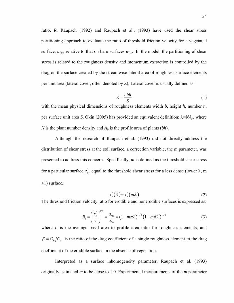
54
ratio, R. Raupach (1992) and Raupach et al., (1993) have used the shear stress
partitioning approach to evaluate the ratio of threshold friction velocity for a vegetated
surface, u*tv, relative to that on bare surfaces u*ts. In the model, the partitioning of shear
stress is related to the roughness density and momentum extraction is controlled by the
drag on the surface created by the streamwise lateral area of roughness surface elements
per unit area (lateral cover, often denoted by λ). Lateral cover is usually defined as:
nbhS
λ = (1)
with the mean physical dimensions of roughness elements width b, height h, number n,
per surface unit area S. Okin (2005) has provided an equivalent definition: λ=NAp, where
N is the plant number density and Ap is the profile area of plants (bh).
Although the research of Raupach et al. (1993) did not directly address the
distribution of shear stress at the soil surface, a correction variable, the m parameter, was
presented to address this concern. Specifically, m is defined as the threshold shear stress
for a particular surface, ''sτ , equal to the threshold shear stress for a less dense (lower λ, m
≤1) surface,:
( ) ( )'' 's s mτ λ τ λ= (2)
The threshold friction velocity ratio for erodible and nonerodible surfaces is expressed as:
( ) ( )
1 2''1 2 1 2*
*
1 1s tst
tv
uR m mu
τ σλ βλτ
− −⎛ ⎞= = = − +⎜ ⎟
⎝ ⎠ (3)
where σ is the average basal area to profile area ratio for roughness elements, and
R SC Cβ = is the ratio of the drag coefficient of a single roughness element to the drag
coefficient of the erodible surface in the absence of vegetation.
Interpreted as a surface inhomogeneity parameter, Raupach et al. (1993)
originally estimated m to be close to 1.0. Experimental measurements of the m parameter
55
by Crawley and Nickling (2003) suggest that m=0.5 to 0.6 when λ is close to 0 and m =
0.2 to 0.3 as λ approaches 0.05. The empirical fit of m=0.16 from Wyatt and Nickling
(1997) is much lower than those of Crawley and Nickling (2003), which may result from
the enhanced effect from wake development downwind of porous vegetation.
Approaching an interpretation of m from the averaged surface shear stress ratio suggests
the original concept of m may be inherently problematic for nonuniform roughness
elements, which cannot be constant over a surface (King et al., 2005).
Several assumptions inherent in the Raupach et al. (1993) shear stress partitioning
model present difficulties in accurate characterizations of stress behavior in vegetated
surfaces. For instance, the m parameter accounts for inhomogeneities in the shear stress
on a vegetated surface, and is intended as a landscape-scale correction factor for these
inhomogeneities. However, shear stress changes as a function of leeward distance from a
shrub (Bradley and Mulhearn, 1983) (fig. 1). A constant m value may not be appropriate
for estimating the inhomogeneous effect of vegetation on the ratio of shear stress on total
bare surfaces. The m parameter is ultimately a correction value based neither on physical
surface characteristics or shear stress theory (Cleugh, 1998).

56
x/h
0 10 20 30 40 50
u * s/ u
*
0.0
0.2
0.4
0.6
0.8
1.0
1.2
Figure 1. The ratio of surface shear velocity to shear velocity u*s/u* for distance downwind of fences expressed in terms of fence heights, x/h, under conditions of neutral thermal stability (from Bradley and Mulhearn, 1983).
Furthermore, in the shear stress partitioning model of Raupach (1992) and
Raupach et al.(1993), lateral cover, λ, describes the density of roughness, but not the
distribution of surface roughness elements. Momentum extraction (Raupach et al., 1993)
and the sheltering effect (Wolfe and Nickling, 1993) are likely to be highly variable in
space, relative to the exact location of vegetation. The size of the sheltered still area in the
lee of vegetation and the extended wake area beyond that are controlled by the height and
width of vegetation (Cleugh, 1998; McNaughton, 1988; Raupach, 1992), and depending
on the lateral and vertical vegetation distribution, the fraction of the ground surface that is
influenced by the wake. Lateral cover, being a simple “landscape scale” parameter,
cannot differentiate between several small objects or a few large objects, nor can lateral

57
cover indicate how vegetation is distributed on the landscape (i.e., randomly, regularly, or
clustered) (figure 2).
Figure 2. The lateral profile of several small roughness elements (bottom) can be the same as the profile area for few large elements (top), but these conditions will provide difference degrees of protection from erosion.
Despite the fact that lateral cover does not specify how vegetation is arranged on
the surface, the use of lateral cover does imply certain factors about how vegetation is
distributed. First, lateral cover implies that vegetation is arranged in well-defined clumps
on the surface with bare areas between these clumps. Second, lateral cover and the σ
ratio in the Raupach et al. (1993) shear stress partitioning model imply that the vegetation
has some easily-defined geometry, specifically with a rectangular profile and, often, a
h
wind direction
h/10

58
round basal area (i.e. cylindrical in form). Third, vegetation is comprised of plants that
are all roughly the same size and geometry, without significant grass cover in the wake of
the mesquite bushes. Fourth, vegetation clumps are randomly arranged.
2. METHODS
2.1. Model description
In this study, we investigate how the spacing of vegetation might be included in
models of aeolian flux to improve predictions of flux from natural surfaces. The new
model, denoted “Q=f(x)”, that we develop uses a probabilistic approach to calculate
landscape-scale horizontal flux, Q, based on fluxes from unvegetated gaps of specific
sizes, q(x), and the probability distribution for unvegetated gaps, p(x):
( ) ( )
0
pQ q x x dx∞
= ∫ (4)
This approach essentially builds on the suggestion by Raupach and Lu (2004) that the
landscape should be divided into homogenous units and be given probabilistic weights
proportional to the relative area of these units.
2.2. Probability of gap size
For modeling purposes, any probability distribution of gap sizes may be used,
however, a distribution that accurately represents the actual gap size distribution is
preferred. Here, we use three different gap-size probability distributions:
1) Gaps are all equal size, L: P(x) =0 x = L1 x ≠ L
⎧ ⎨ ⎩
(5)

59
2) Gap size is defined by a Poisson distribution with the most likely gap size equal to L
and an average gap size equal to L = L :
P(x) =
e−LLx
x! (6)
3) Gap size is defined by the following curve with the most likely gap size equal to L:
∫∞
−
−
=
0
)(dxxe
xexPx
L
xL
(7)
This probability distribution is derived from an exponential decrease in gap
“connectivity” observed by (McGlynn and Okin, 2006). For this distribution and all
other arbitrary gap size probability distributions, the average gap size, L , is equal to:
L = xP(x)dx
0
∞
∫ (8)
A relationship exists between the average gap size for any probability distribution,
L , and lateral cover, λ. Consider a line transect across vegetation arranged in columnar
clumps, all of roughly the same size. The average length of a gap and the adjacent
(upwind) plant, D, will be given by:
D = L + W (9)where W is the average streamwise width of a plant and, L is the average streamwise
width of a gap. For a circle of diameter d = 1 m, W = 0.574d , as the probability of a line
intersecting any point within the circle basal area.
Based on these definitions, the number density of plants in the streamwise
direction is given simply by N = D( )−1. The fractional cover of plants, C, is the fraction of
the length of a line parallel to the direction of the wind that is covered by plants, and is
given by:

60
C =
WL + W
= W N (10)
Okin (2005) and Lancaster and Baas (1998) have shown that relationship exists between
C, and lateral cover λ:
λ =AP
AB
C (11)
where AP is the average profile area of plants, and AB is the average basal area of plants.
For cylindrical plants, the basal area is equal πd2/4 and the profile area, is given by dh.
Thus, the ratio for these plants of AP/AB is given by (4/π)(h/d). Combining equation 11
with the definition of C yields:
λ =
AP WAB L + W( )
(12)
Rearranging to solve for L yields a relationship between L and λ:
L = W AP
AB λ−1
⎛
⎝ ⎜
⎞
⎠ ⎟ (13)
The relationship between L and λ is plotted in figure 3.

61
λ
0.0 0.2 0.4 0.6 0.8 1.0
_ L
0
10
20
30
Figure 3. The average streamwise width ( L ) versus lateral cover (λ), assuming diameter d=1,W = 0.574d , and plant area ratio AP/AB=1. 2.3. Horizontal flux
Based on considerations of conservation of momentum under steady-state
saltation (Shao et al., 1993), horizontal dust flux is modeled as:
q = Ku* u*2 − u*tv
2( ) (13)when u* exceeds the threshold shear velocity, u*tv, and where K A gρ= , A is a
dimensionless constant with value approximately equal to 1, ρ is the density of air, and g
is the acceleration due to gravity. In our model, we modify equation (13) slightly, so that
q and u*tv are functions of gap size, x:
q(x) = Ku* u*2 − (u*tv (x))2( ) (14)
Rearranging equation 3 and expressing m as a function of gap size returns a distance
dependent threshold friction velocity for vegetated surfaces.

62
( )( )* *( ) 1 ( ) 1 ( )tv tsu x u m x m xσλ βλ= − + (15)
Shear stress changes as a function of leeward distance from a shrub resulting from
nonerodible sheltered areas, and the creation of downwind wakes (fig. 4). With changes
in shear stress with distance, m cannot be assumed to be constant, but is instead a
function of gap size: ( ) ( )m x f x= . Fences have long been erected as barriers to stabilize
soil and reduce wind erosion. As solid and semi-permeable structures, fences can
represent many of the roughness-sheltering behaviors observed in vegetation. Like
vegetation, fences create downstream wakes, with porous fences more effective in
sheltering erodible surfaces than solid buffers (Bradley and Mulhearn, 1983). The
sheltered areas experience reduced turbulence, in addition to decreased water vapor and
CO2 flux, and reduced sandblasting (Cleugh, 1998). The sheltering influence of
vegetation decreases with distance, with a sheltered area in the immediate downwind
shadow of the fence and an extended wake area extended beyond the sheltered area.
Figure 4. Surface barriers such as fences or vegetation create sheltered areas and the development of downwind wakes (from McNaughton, 1988).
0 4 8 12 16
x/h
h
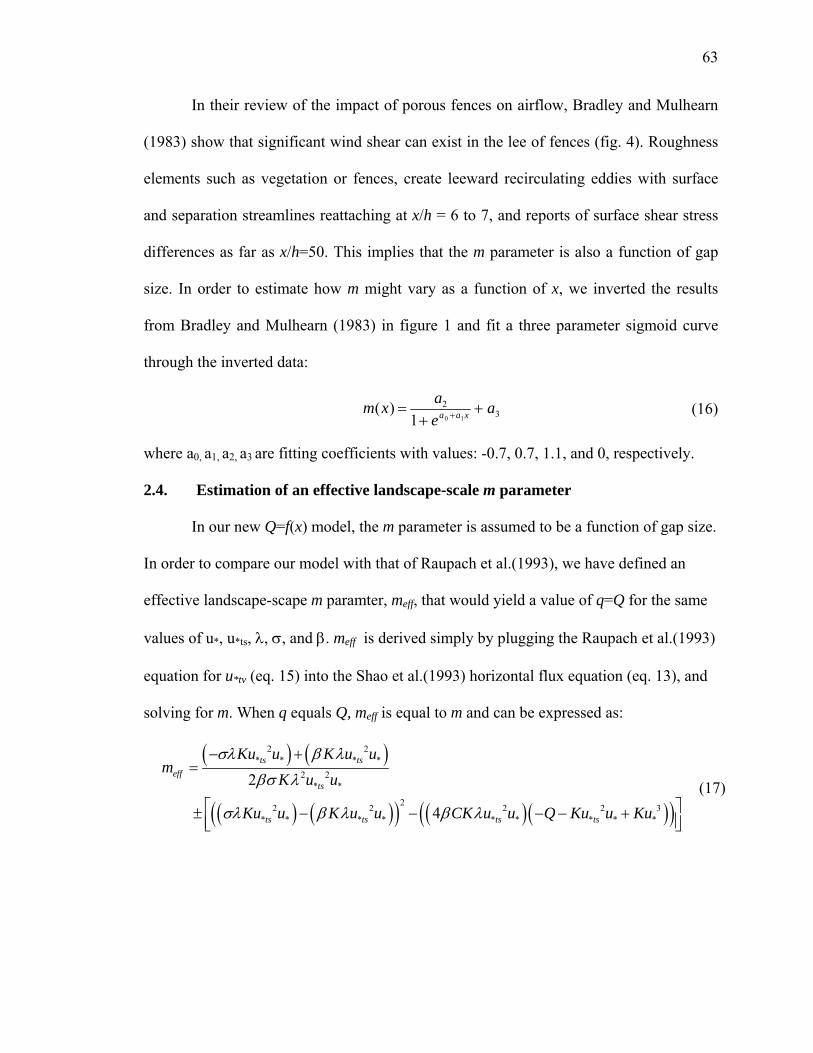
63
In their review of the impact of porous fences on airflow, Bradley and Mulhearn
(1983) show that significant wind shear can exist in the lee of fences (fig. 4). Roughness
elements such as vegetation or fences, create leeward recirculating eddies with surface
and separation streamlines reattaching at x/h = 6 to 7, and reports of surface shear stress
differences as far as x/h=50. This implies that the m parameter is also a function of gap
size. In order to estimate how m might vary as a function of x, we inverted the results
from Bradley and Mulhearn (1983) in figure 1 and fit a three parameter sigmoid curve
through the inverted data:
m(x) =a2
1+ ea0 +a1x + a3 (16)
where a0, a1, a2, a3 are fitting coefficients with values: -0.7, 0.7, 1.1, and 0, respectively.
2.4. Estimation of an effective landscape-scale m parameter
In our new Q=f(x) model, the m parameter is assumed to be a function of gap size.
In order to compare our model with that of Raupach et al.(1993), we have defined an
effective landscape-scape m paramter, meff, that would yield a value of q=Q for the same
values of u*, u*ts, λ, σ, and β. meff is derived simply by plugging the Raupach et al.(1993)
equation for u*tv (eq. 15) into the Shao et al.(1993) horizontal flux equation (eq. 13), and
solving for m. When q equals Q, meff is equal to m and can be expressed as:
( ) ( )
( ) ( )( ) ( )( )( )
2 2* * * *
2 2* *
22 2 2 2 3* * * * * * * * *
2
4
ts tseff
ts
ts ts ts ts
Ku u K u um
K u u
Ku u K u u CK u u Q Ku u Ku
σλ β λ
βσ λ
σλ β λ β λ
− +=
⎡ ⎤± − − − − +⎢ ⎥⎣ ⎦
(17)

64
2.5. Field observations
Flux observations from Big Spring Number Eight (BSNES) collectors were
recorded in the Chihuahuan Desert of southern New Mexico at Jornada Experimental
Range (JER) for a period of approximately 3 months during the spring and summer of
2005. Simultaneous measurements of vegetation allowed estimation of the mean gap size,
L (fig.5). Similar results have also been reported from Lancaster and Baas (1998) from a
low vegetation sandsheet in dried Owens Lake, California (fig. 6). These results will be
used here, along with field results from Jornada as a preliminary check of the model
presented here.
_L (m)
0 2 4 6 8
Q (g
m-2
d-1
)
0
100
200
300
400
spring 2005summer 2005
Figure 5. Dust flux versus mean gap size observed at the Jornada Experimental Range, NM during a three month period in the spring and summer of 2005.

65
λ
0.00 0.05 0.10 0.15 0.20 0.25
Q (g
m-2
s-1
)
0.0
0.2
0.4
0.6
0.8
1.0
03/27/1996 01/26/1996 12/18/1995 11/30/1995 01/02/1996 01/22/1996
Figure 6. Flux events for lateral cover expressed in range from Owens Lake, CA (modified from Lancaster and Baas, 1998). 3. RESULTS
Estimates of Q vs. λ and Q vs. L were made with the Q=F(x) model for the
following conditions:
• Wind shear velocity: u*=120 cm s-1
• Threshold shear velocity of the unvegeted soil: u*ts = 25 cm s-1
• Plant geometry: 0.5 m tall cylinders with a 1 m diameter
• Drag coefficient ratio: β = 269 calculated as Cr/Cs, Cr=0.485 (Gillies et al., 2002;
Wyatt and Nickling, 1997), Cs=0.0018 (Marshall, 1971)
To compare results from the Q=f(x) model with the existing Raupach et al. (1993) model,
we have also calculated the horizontal flux under the above conditions for constant value
of m=0.5 and m=1.0.

66
Three gap probability functions were used in the Q=f(x) model. Presented as
equations 5-7, each distribution represents different scenarios of surface vegetation (fig.
7). The majority of dust models assume homogeneous or random distributions of
vegetation (Gillette and Stockton, 1989; Marticorena and Bergametti, 1995; Musick and
Gillette, 1990a). In the uniform gap model, all gap sizes are assumed to have the same
windward length. This scenario is unlikely due to natural variability of vegetation sizes at
different times, at difference stages of growth, especially from a mosaic ecological
perspective (Caylor et al., 2003), and due to inhomogeneous environmental limitations
such as nutrient availability, soil moisture, and topography. However, the case of constant
gap size is illustrative of how gap size influences model estimates of horizontal flux.
With uniform gap spacing, flux is effectively suppressed in when the average streamwise
gap width is less than 4 m or when the lateral cover exceeds 0.09.
Vegetation in natural systems is not composed of discrete sizes and constant gap
distances, but of a continuous distribution of sizes and shapes. Gap size variations are
represented as a normalized Poisson distribution (eq. 6). The gap distribution was
normalized after eliminated distances with a probably less than 0.025. Highly variable
gap sizes between plants would be expected in most natural systems due to variability in
nutrient availability, soil moisture, and topography. With variable gap spacing from the
Poisson distribution would be expected to demonstrate more complex behavior than the
simple threshold behavior observed in the constant gap-size model. With the Poisson
distribution, we observe that the decrease with lateral cover is moderated with detectible
emissions at 3>L m, and λ > 0.16. Dust emissions are expected over a wide range of
average gap sizes.

67
A third distribution was developed from the probability of adjacent areas having
the same landcover. Based on the connectivity statistic (McGlynn and Okin, 2006), a
distribution similar to an exponential decay function, the gap size is calculated from the
range value (eq. 7). In this approach, distances with a probability less than 0.015 were
eliminated, and the distribution was normalized against the remaining lag distances. With
connectivity gap spacing, dust emissions are theoretically possible at large ranges. At
higher range values, the gap sizes can be as large as 30 m. Such large gaps are unlikely,
due to natural constraints on vegetation. Additionally, including emissions from such
high gap distances (> 20 m) is likely to overestimate dust emission in natural systems.

68
uniform distribution
p(x)
0.0
0.2
0.4
0.6
0.8
1.0
range=1range=5range=10
Poisson distribution
p(x)
0.0
0.2
0.4
connectivity distribution
range (m)
0 10 20 30
p(x)
0.0
0.2
0.4
Figure 7. Gap spacing at ranges distances of 1, 7, and 10 m for uniform gap distribution, Poison gap distribution, and connectivity gap distribution.

69
Total flux (Q) is calculated for lateral cover based on the horizontal flux
approximations (eq. 14), and the flux-probability relationship (eq. 4). In all three modeled
distributions (eqs. 5-7), dust flux calculated at u*=150 cm s-1 is highest for surfaces with
minimal lateral cover (fig. 8). Flux is effectively suppressed in the uniform distribution
when the average streamwise gap width is less than 4 m or when the lateral cover exceeds
λ = 0.09. Dust flux is possible for almost any patch-size scale length with Poisson and
connectivity distributions, and remains present beyond surfaces with high lateral cover
λ > 0.3, but is greatly reduced when λ ≤ 0.15.
λ
0.0 0.1 0.2 0.3 0.4
Q (g
cm
-2 s
-1)
0
1
2
3
4uniform distributionPoisson distributionconnectivity distribution
Figure 8. Probability of total dust emissions for uniform gap distribution, Poison gap distribution, and connectivity gap distribution.
Performance of the dust flux model for vegetated surfaces was evaluated against
field results taken in the Jornada Experimental Range (JER), NM, and published field
data from Lancaster and Baas (1998). Expressed as the ratio of dust flux relative to

70
maximum potential flux, high relative flux is reported from field data at λ < 0.04, with
the lowest results from the mean Lancaster and Baas (1998) observations (fig. 9). Flux
observations decrease sharply for JER field data with high emissions at λ = 0.09. For
both sets of field data, flux emissions decrease sharply at 0.1λ ≈ as lateral cover reaches
a critical density. Significant emissions are still possible at higher cover, with JER
observations at λ = 0.32 and λ = 0.46. The Raupach model for a stable highly-vegetated
surface (m=1.0) and for the recommended value from Crawley and Nickling (2003)
(m=0.55) for low cover (λ→0), that also approximates the Raupach value for an erodible
bare surface (m=0.5), approximates the initial Lancaster and Baas (1998) observation at
low lateral cover (λ = 0.04), but fails to account for emissions at λ > 0.1. Of the three
distribution models, the uniform gap size distribution most closely matches JER field
observations, but fails to predict flux probabilities at λ > 0.09. The Poisson distribution
correctly matches connectivity predictions, but with higher flux estimates at high cover
(λ ≥ 0.15). The flux estimate for connectivity distributions accounts for emissions at high
cover (λ > 0.3) but underestimates flux as λ~0.4.

71
λ
0.0 0.1 0.2 0.3 0.4 0.5
Qca
lc\ Q
max
0.0
0.2
0.4
0.6
0.8
1.0Raupach (m=1.0)Raupach (m=0.55)uniform distributionPoisson distributionconnectivity distributionLancaster & Baasspring 2005summer 2005
Figure 9. Dust emission models (lines) and field observations (points). Constant m models from Raupach et al. (1993) underestimate dust flux for vegetated surfaces with λ > 0.2.
When vegetation is projected as gap size, both Raupach models continuously
underestimate flux probability (fig. 10). The Poisson and connectivity distributions
successfully predict emissions at small gap sizes (~ 2.5 m) as observed in Lancaster and
Baas (1998), and in both summer and spring 2005 JER. Only the Poison distribution
accurately estimates the JER field emission with gap sizes between 3.5 and 7.5 m. In this
range, the uniform distribution strongly overestimates horizontal flux, while the
connectivity distribution underestimates horizontal flux.

72
_L (m)
0 5 10 15 20
Qca
lc/ Q
max
0.0
0.2
0.4
0.6
0.8
1.0
Figure 10. Modeled dust flux from the Poisson distribution closely matches observed field emissions. Constant m models underestimate flux for all gap sizes.
Raupach (m=1)Raupach (m=0.55)uniform distributionPoisson distributionConnectivity distributionLancaster & Baasspring 2005summer 2005
4. DISCUSSION AND CONCLUSIONS
We have presented a new model for dust flux, with shear stress inhomogeneity of
vegetation for comparison with theoretical and field based experiments. The Q=f(x)
model, based on field observations of dust flux versus mean gap size, and from published
surface shear stress response to porous roughness elements, confirms surfaces stress
inhomogeneity (m) is not constant with lateral cover and cannot be easily estimated from
coarse vegetation classifications, such as bare soil, or stabilized vegetated surface.
Traditional approximations of the m parameter are no longer valid and cannot be applied

73
from existing literature. Surface shear stress for vegetated surfaces was found to have a
non-linear relationship with gap size suggesting possible wake interference at moderate
densities of λ=0.1.
Surface roughness elements such as vegetation have long been recognized as
moderators of wind erosion, affecting the erodibility of the surface and the entrainment of
dust particles in arid environments. Experimental and theoretical research has
demonstrated the reduction in wind erosion from vegetation by creating nonerodible
surface areas, extracting wind momentum, developing downwind wakes, and capturing
moving particles. A primary attribute of wind erosion reduction, is from the suppression
of horizontal flux by vegetation in the form of saltation to the point where vertical dust
entrainment is no longer produced.
Wind blowing over a vegetated surface is not just affected by the geometry of
vegetation, but also by the spacing between plants. In surfaces with a high-density of
vegetation, entrainment is greatly reduced. If the spacing between vegetation is increased,
the saltation suppression of a single plant is reduced as the wind velocity and shear stress
is able increase with distance, without a succeeding downwind roughness element. Field
data and experimental results in figure 10 clearly demonstrate an increase in dust flux as
average gap size increase on a scale from 0 to 10 m. The spacing of vegetation in most
scenarios is not expected to be constant, lending more credence to the Poisson and
connectivity distributions over the uniform gap size distribution, although any
appropriate distribution may be applied to this model.
Incorporating vegetation gap size into the dust flux model overcomes problems
associated with the use of lateral cover in the original Raupach et al. (1993) model.

74
Integrating the spatial distribution of vegetation with lateral cover allows a more robust
representation of the surface in wind erosion that is missing from existing models.
In existing wind shear stress models (e.g., Raupach et al, 1993), the m parameter
provides a proxy for inhomogenous shear stress. Nonlinear trends of meff with lateral
cover imply that no single value of m can be used for a wide range of vegetation
roughness densities (fig. 11).
The protective characteristics of vegetation are minimized when sparse lateral
cover (λ < 0.08) and large mean gap sizes prevent overlapping shelters and wake effects
from adjacent plants. In high density vegetation (λ > 0.25), a skimming flow, described in
Wolfe and Nickling (1993), of continuously overlapping wake regions would also result
in a relatively homogeneous surface shear stress, and even moderate distributions would
have little measurable effect.
In scenarios of moderate gap sizes and lateral cover ( 0.08 0.25λ< < ), wake
interference flow is created, producing highly inhomogeneous surface shear stress. The
transitional nature of surface shear stress inhomogeneity is demonstrated as the
homogeneous wind flow regime for sparse uniform vegetation becomes highly distorted
with interference wakes at λ = 0.8. As λ increases to 2.5, the wakes overlap, creating
large sheltered areas of homogeneous flow.

75
λ
0.0 0.1 0.2 0.3 0.4
mef
f
0.0
0.1
0.2
0.3
0.4
0.5
0.6uniform distributionPoisson distributionconnectivity distribution
Figure 11. Natural variability in vegetation distributions in very low and high densities are minimally affect shear stress inhomogeneity while moderate densities create highly variable shear stress distributions from wake interference flow, represented with 3rd-order polynomials.
Scaling effects of inhomogeneity and vegetation distribution may account for
some discrepancies between modeled dust flux and field observations. Spatially averaged
calculations cannot reflect natural variation in vegetation distribution measured at a
single location. Larger sample sizes may produce measured values that approximate
theoretical mean spatial characteristics.
Changes in shear stress with distance and varying gap size prevent the
development of a constant m inhomogeneity parameter. The variation in m parameters for
seemingly similar surfaces may explain why so much research has such difficulty and
inconsistency in developing practical solutions. Recent findings by King et al. (2005)
suggests that shear stress partitioning overestimations require a modification of the m
parameter from a scaling term. The semi-empirical estimation of the m parameter

76
suggested here agrees with existing field results, may represent averaged shear stress.
This presents a method for consistent m estimations amongst literature, and could
improve future dust modeling.
A larger dataset of flux emissions measured at different scales with detailed
measurements of vegetation geometry and distribution is necessary to permit accurate
comparison between field results and theoretical predictions. Such data may not be
common, but measures of gap size from field sites, or from air and space based remote
sensing imagery may enhance the predictive erodibility of vegetated surfaces.
For the present purpose, the m parameter is depicted as a modifier of shear stress
resulting from the spatial distribution of maximum shear stress. The resulting m
assumption, from a sigmoid fit of Bradley and Mulhearn (1983) is not based on
experiments or theoretical considerations that were conducted with the intention of
identifying how shear stress varies with distance from a plant. The actual shape of the
( , ), ( )q f x m m f x= = function, and how it might vary with plant porosity is unknown.
In addition, several assumptions for ambient conditions were used in this study as
constant wind shear velocity that limit the comparison of model results with field results.
Despite the general agreement from the Q=f(x) model with JER field data, and with
Lancaster and Baas (1998) field observations, only general predictions are possible.
Detailed surface shear stress and wind records would be necessary to transition from
general estimations, into accurate landscape-scale predictions and validation of this
model.
77
CITED REFERENCES Alfaro, S. C., and Gomes, L. (2001). Modeling mineral aerosol production by wind
erosion: Emission intensities and aerosol size distributions in source areas.
Journal of Geophysical Research-Atmospheres 106, 18075-18084.
Ansley, R. J., Ben Wu, X., and Kramp, B. A. (2001). Observation: Long-term increases
in mesquite canopy cover in a North Texas savanna. Journal of Range
Management 54, 171-176.
Archer, S. (1995). Tree-grass dynamics in a prosopis-thornscrub savanna parkland -
reconstructing the past and predicting the future. Ecoscience 2, 83-99.
Baatz, M., and Schäpe, A. (2000). "Multiresolution segmentation: An optimization for
high quality multi-scale image segmentation." Wichmann-Verlag, Heidelberg.
Bagnold, R. A. (1941). "The physics of blown sand and desert dunes." Methuen & Co.,
London.
Bahre, C. J., and Shelton, M. L. (1993). Historic vegetation change, mesquite increases,
and climate in Southeastern Arizona. Journal of Biogeography 20, 489-504.
Baker, A. R., Jickells, T. D., Witt, M., and Linge, K. L. (2006). Trends in the solubility of
iron, aluminium, manganese and phosphorus in aerosol collected over the Atlantic
Ocean. Marine Chemistry 98, 43-58.
Baret, F., and Guyot, G. (1991). Potentials and limits of vegetation indexes for LAI and
APAR assessment. Remote Sensing of Environment 35, 161-173.
Bellouin, N., Boucher, O., Haywood, J., and Reddy, M. S. (2005). Global estimate of
aerosol direct radiative forcing from satellite measurements. Nature 438, 1138-
1141.

78
Bishop, J. K. B., Davis, R. E., and Sherman, J. T. (2002). Robotic observations of dust
storm enhancement of carbon biomass in the North Pacific. Science 298, 817-821.
Bour, O., and Davy, P. (1998). On the connectivity of three-dimensional fault networks.
Water Resources Research 34, 2611-2622.
Bradley, B. A., and Mustard, J. F. (2005). Identifying land cover variability distinct from
land cover change: Cheatgrass in the Great Basin. Remote Sensing of Environment
94, 204-213.
Bradley, E. F., and Mulhearn, P. J. (1983). Development of velocity and shear stress
distributions in the wake of a porous shelter fence. Journal of Wind Engineering
and Industrial Aerodynamics 15, 145-156.
Buffington, L. C., and Herbel, C. H. (1965). Vegetational changes on a semidesert
grassland range from 1858 to 1963. Ecological Monographs 35, 139-164.
Bullard, J. E. (1997). A note on the use of the ''Fryberger Method'' for evaluating
potential sand transport by wind. Journal of Sedimentary Research 67, 499-501.
Cabral, A. C., De Miguel, J. M., Rescia, A. J., Schmitz, M. F., and Pineda, F. D. (2003).
Shrub encroachment in Argentinean savannas. Journal of Vegetation Science 14,
145-152.
Caylor, K. K., Dowty, P. R., Shugart, H. H., and Ringrose, S. (2004). Relationship
between small-scale structural variability and simulated vegetation productivity
across a regional moisture gradient in southern Africa. Global Change Biology
10, 374-382.

79
Caylor, K. K., Shugart, H. H., Dowty, P. R., and Smith, T. M. (2003). Tree spacing along
the Kalahari transect in southern Africa. Journal of Arid Environments 54, 281-
296.
Chadwick, O. A., Derry, L. A., Vitousek, P. M., Huebert, B. J., and Hedin, L. O. (1999).
Changing sources of nutrients during four million years of ecosystem
development. Nature 397, 491-497.
Cleugh, H. A. (1998). Effects of windbreaks on airflow, microclimates and crop yields.
Agroforestry Systems 41, 55-84.
Cornelis, W. M., and Gabriels, D. (2003). The effect of surface moisture on the
entrainment of dune sand by wind: an evaluation of selected models.
Sedimentology 50, 771-790.
Cotner, J. B., Ammerman, J. W., Peele, E. R., and Bentzen, E. (1997). Phosphorus-
limited bacterioplankton growth in the Sargasso Sea. Aquatic Microbial Ecology
13, 141-149.
Crawley, D. M., and Nickling, W. G. (2003). Drag partition for regularly-arrayed rough
surfaces. Boundary-Layer Meteorology 107, 445-468.
D'Odorico, P., Porporato, A., and Ridolfi, L. (2001). Transition between stable states in
the dynamics of soil development. Geophysical Research Letters 28, 595-598.
Deutsch, C. V., and Journel, A. G. (1998). "GSLIB. Geostatistical software library and
users guide." Oxford University Press, New York.
Diaz, J. P., Exposito, F. J., Torres, C. J., Herrera, F., Prospero, J. M., and Romero, M. C.
(2001). Radiative properties of aerosols in Saharan dust outbreaks using ground-

80
based and satellite data: Applications to radiative forcing. Journal of Geophysical
Research-Atmospheres 106, 18403-18416.
Diner, D. J., Asner, G. P., Davies, R., Knyazikhin, Y., Muller, J. P., Nolin, A. W., Pinty,
B., Schaaf, C. B., and Stroeve, J. (1999). New directions in earth observing:
Scientific applications of multiangle remote sensing. Bulletin of the American
Meteorological Society 80, 2209-2228.
Dorren, L. K. A., Maier, B., and Seijmonsbergen, A. C. (2003). Improved Landsat-based
forest mapping in steep mountainous terrain using object-based classification.
Forest Ecology And Management 183, 31-46.
Dougill, A. J., and Thomas, A. D. (2004). Kalahari sand soils: Spatial heterogeneity,
biological soil crusts and land degradation. Land Degradation & Development 15,
233-242.
Dregne, H. E., and Chou, H. T. (1992). "Global desertification dimensions and costs."
Texas Tech University Press, Lubbock, Texas.
Farr, T. G., and Chadwick, O. A. (1996). Geomorphic processes and remote sensing
signatures of alluvial fans in the Kun Lun mountains, China. Journal of
Geophysical Research-Planets 101, 23091-23100.
Fensham, R. J., Fairfax, R. J., and Archer, S. R. (2005). Rainfall, land use and woody
vegetation cover change in semi-arid Australian savanna. Journal of Ecology 93,
596-606.
Geneletti, D., and Gorte, B. G. H. (2003). A method for object-oriented land cover
classification combining Landsat TM data and aerial photographs. International
Journal of Remote Sensing 24, 1273-1286.
81
Gibbens, R. P., McNeely, R. P., Havstad, K. M., Beck, R. F., and Nolen, B. (2005).
Vegetation changes in the Jornada Basin from 1858 to 1998. Journal of Arid
Environments 61, 651-668.
Gillette, D. (1997). Soil derived dust as a source of silica: Aerosol properties, emissions,
deposition, and transport. Journal of Exposure Analysis and Environmental
Epidemiology 7, 303-311.
Gillette, D. A., Herbert, G., Stockton, P. H., and Owen, P. R. (1996). Causes of the fetch
effect in wind erosion. Earth Surface Processes and Landforms 21, 641-659.
Gillette, D. A., and Pitchford, A. M. (2004). Sand flux in the northern Chihuahuan desert,
New Mexico, USA, and the influence of mesquite-dominated landscapes. Journal
of Geophysical Research-Earth Surface 109.
Gillette, D. A., and Stockton, P. H. (1989). The effect of nonerodible particles on wind
erosion of erodible surfaces. Journal of Geophysical Research-Atmospheres 94,
12885-12893.
Gillies, J. A., Nickling, W. G., and King, J. (2002). Drag coefficient and plant form
response to wind speed in three plant species: Burning Bush (Euonymus alatus),
Colorado Blue Spruce (Picea pungens glauca.), and Fountain Grass (Pennisetum
setaceum). Journal of Geophysical Research-Atmospheres 107,
doi:10.1029/2001JD001259.
Gomes, L., Bergametti, G., Coudegaussen, G., and Rognon, P. (1990). Submicron desert
dusts - a sandblasting process. Journal of Geophysical Research-Atmospheres 95,
13927-13935.
82
Greeley, R., and Iversen., J. D. (1985). "Wind as a geological process: on Earth, Mars,
Venus, and Titan." Cambridge University Press, Cambridge.
Haywood, J., and Boucher, O. (2000). Estimates of the direct and indirect radiative
forcing due to tropospheric aerosols: A review. Reviews of Geophysics 38, 513-
543.
Houghton, J. T., Ding, Y., Griggs, D. J., Noguer, M., van der Linden, P. J., Dia, X.,
Maskell, K., and Johnson, C. A. (2001). "Climate change 2001: the scientific
basis: contribution of Working Group I to the third assessment report of the
Intergovernmental Panel on Climate." Cambridge University Press, New York.
Huete, A., Didan, K., Miura, T., Rodriguez, E. P., Gao, X., and Ferreira, L. G. (2002).
Overview of the radiometric and biophysical performance of the MODIS
vegetation indices. Remote Sensing of Environment 83, 195-213.
Husar, R. B., Prospero, J. M., and Stowe, L. L. (1997). Characterization of tropospheric
aerosols over the oceans with the NOAA advanced very high resolution
radiometer optical thickness operational product. Journal of Geophysical
Research-Atmospheres 102, 16889-16909.
Karyampudi, V. M., Palm, S. P., Reagen, J. A., Fang, H., Grant, W. B., Hoff, R. M.,
Moulin, C., Pierce, H. F., Torres, O., Browell, E. V., and Melfi, S. H. (1999).
Validation of the Saharan dust plume conceptual model using lidar, Meteosat, and
ECMWF data. Bulletin of the American Meteorological Society 80, 1045-1075.
Kaufman, Y. J., Tanre, D., and Boucher, O. (2002). A satellite view of aerosols in the
climate system. Nature 419, 215-223.

83
King, J., Nickling, W. G., and Gillies, J. A. (2005). Representation of vegetation and
other nonerodible elements in aeolian shear stress partitioning models for
predicting transport threshold. Journal of Geophysical Research-Earth Surface
110, doi:10.1029/2004JF000281.
King, M. D., Kaufman, Y. J., Tanre, D., and Nakajima, T. (1999). Remote sensing of
tropospheric aerosols from space: Past, present, and future. Bulletin of the
American Meteorological Society 80, 2229-2259.
Krishnan, S., and Journel, A. G. (2003). Spatial connectivity: From variograms to
multiple-point measures. Mathematical Geology 35, 915-925.
Laliberte, A. S., Rango, A., Havstad, K. M., Paris, J. F., Beck, R. F., McNeely, R., and
Gonzalez, A. L. (2004). Object-oriented image analysis for mapping shrub
encroachment from 1937 to 2003 in southern New Mexico. Remote Sensing of
Environment 93, 198-210.
Lancaster, N., and Baas, A. (1998). Influence of vegetation cover on sand transport by
wind: Field studies at Owens Lake, California. Earth Surface Processes and
Landforms 23, 69-82.
Leys, J. F., and McTainsh, G. H. (1996). Sediment fluxes and particle grain-size
characteristics of wind-eroded sediments in southeastern Australia. Earth Surface
Processes and Landforms 21, 661-671.
Li, J., Okin, G. S., Hartman, L. J., and Epstein, H. E. (submitted). Quantitative
assessment of wind erosion and soil nutrient loss in desert grasslands of the
southwestern United States. Biogeochemistry.

84
Li, X., Maring, H., Savoie, D., Voss, K., and Prospero, J. M. (1996). Dominance of
mineral dust in aerosol light-scattering in the North Atlantic trade winds. Nature
380, 416-419.
Liao, H., and Seinfeld, J. H. (1998). Effect of clouds on direct aerosol radiative forcing of
climate. Journal of Geophysical Research-Atmospheres 103, 3781-3788.
Liao, H., Yung, Y. L., and Seinfeld, J. H. (1999). Effects of aerosols on tropospheric
photolysis rates in clear and cloudy atmospheres. Journal of Geophysical
Research-Atmospheres 104, 23697-23707.
Mahowald, N. M., Baker, A. R., Bergametti, G., Brooks, N., Duce, R. A., Jickells, T. D.,
Kubilay, N., Prospero, J. M., and Tegen, I. (2005). Atmospheric global dust cycle
and iron inputs to the ocean. Global Biogeochemical Cycles 19,
doi:10.1029/2004GB002402.
Marshall, J. K. (1971). Drag measurements in roughness arrays of varying density and
distribution. Agricultural Meteorology 8, 269-292.
Marticorena, B., and Bergametti, G. (1995). Modeling the atmospheric dust cycle.1.
Design of a soil-derived dust emission scheme. Journal of Geophysical Research-
Atmospheres 100, 16415-16430.
McGlynn, I. O., and Okin, G. S. (2006). Characterization of shrub distribution using high
spatial resolution remote sensing: Ecosystem implications for a former
Chihuahuan Desert grassland. Remote Sensing of Environment 101, 554-566.
McNaughton, K. G. (1988). Effects of windbreaks on turbulent transport and
microclimate. Agriculture Ecosystems & Environment 22-3, 17-39.

85
Miller, R. L., Perlwitz, J., and Tegen, I. (2004). Feedback upon dust emission by dust
radiative forcing through the planetary boundary layer. Journal of Geophysical
Research-Atmospheres 109, doi:10.1029/2003GL018279.
Musick, H., and Gillette, D. (1990a). Field evaluation of relationships between a
vegetations structural parameter and sheltering against wind erosion. Land
Degredation Rehab. 2, 87-94.
Musick, H. B., and Gillette, D. A. (1990b). Field evaluation of relationships between a
vegetation structural parameter and sheltering against wind erosion. Land
Degradation and Rehabilitation 2, 87-94.
Okin, G. S. (2005). Dependence of wind erosion and dust emission on surface
heterogeneity: Stochastic modeling. Journal of Geophysical Research-
Atmospheres 110, doi:10.1029/2004JD005288.
Okin, G. S., and Gillette, D. A. (2001). Distribution of vegetation in wind-dominated
landscapes: Implications for wind erosion modeling and landscape processes.
Journal of Geophysical Research-Atmospheres 106, 9673-9683.
Okin, G. S., Mahowald, N., Chadwick, O. A., and Artaxo, P. (2004). Impact of desert
dust on the biogeochemistry of phosphorus in terrestrial ecosystems. Global
Biogeochemical Cycles 18, doi:10.1029/2003GB002145.
Okin, G. S., Murray, B., and Schlesinger, W. H. (2001a). Degradation of sandy arid
shrubland environments: observations, process modelling, and management
implications. Journal of Arid Environments 47, 123-144.
Okin, G. S., and Painter, T. H. (2004). Effect of grain size on remotely sensed spectral
reflectance of sandy desert surfaces. Remote Sensing of Environment 89, 272-280.

86
Okin, G. S., Roberts, D. A., Murray, B., and Okin, W. J. (2001b). Practical limits on
hyperspectral vegetation discrimination in arid and semiarid environments.
Remote Sensing of Environment 77, 212-225.
Phinn, S., Franklin, J., Hope, A., Stow, D., and Huenneke, L. (1996). Biomass
distribution mapping using airborne digital video imagery and spatial statistics in
a semi-arid environment. Journal of Environmental Management 47, 139-164.
Poggi, D., Katul, G. G., and Albertson, J. D. (2004). A note on the contribution of
dispersive fluxes to momentum transfer within canopies. Boundary-Layer
Meteorology 111, 615.
Privette, J. L., Tian, Y., Roberts, G., Scholes, R. J., Wang, Y., Caylor, K. K., Frost, P.,
and Mukelabai, M. (2004). Vegetation structure characteristics and relationships
of Kalahari woodlands and savannas. Global Change Biology 10, 281-291.
Prospero, J. M., and Lamb, P. J. (2003). African droughts and dust transport to the
Caribbean: Climate change implications. Science 302, 1024-1027.
Pye, K. (1987). "Aeolian Dust and Dust Deposits." Academic Press, London.
Rango, A., Chopping, M., Ritchie, J., Havstad, K., Kustas, W., and Schmugge, T. (2000).
Morphological characteristics of shrub coppice dunes in desert grasslands of
southern New Mexico derived from scanning LIDAR. Remote Sensing of
Environment 74, 26-44.
Rango, A., Goslee, S., Herrick, J., Chopping, M., Havstad, K., Huenneke, L., Gibbens,
R., Beck, R., and McNeely, R. (2002). Remote sensing documentation of historic
rangeland remediation treatments in southern New Mexico. Journal of Arid
Environments 50, 549-572.

87
Raupach, M. R. (1991). Vegetation-atmosphere interaction in homogeneous and
heterogeneous terrain - Some implications of mixed-layer dynamics. Vegetatio
91, 105-120.
Raupach, M. R. (1992). Drag and drag partition on rough surfaces. Boundary-Layer
Meteorology 60, 375-395.
Raupach, M. R. (1994). Simplified expressions for vegetation roughness length and zero-
plane displacement as functions of canopy height and area index. Boundary-Layer
Meteorology 71, 211-216.
Raupach, M. R., Gillette, D. A., and Leys, J. F. (1993). The effect of roughness elements
on wind erosion threshold. Journal of Geophysical Research-Atmospheres 98,
3023-3029.
Raupach, M. R., and Lu, H. (2004). Representation of land-surface processes in aeolian
transport models. Environmental Modelling & Software 19, 93-112.
Raupach, M. R., Woods, N., Dorr, G., Leys, J. F., and Cleugh, H. A. (2001). The
entrapment of particles by windbreaks. Atmospheric Environment 35, 3373-3383.
Ravi, S., and D'Odorico, P. (2005). A field-scale analysis of the dependence of wind
erosion threshold velocity on air humidity. Geophysical Research Letters 32,
doi:10.1029/2005GL023675.
Ravi, S., D'Odorico, P., Over, T. M., and Zobeck, T. M. (2004). On the effect of air
humidity on soil susceptibility to wind erosion: The case of air-dry soils.
Geophysical Research Letters 31, doi:10.1029/2004GL019485.
88
Ravi, S., Zobeck, T. M., Over, T. M., Okin, G. S., and D'Odorico, P. (in press). On the
effect of moisture bonding forces in air-dry soils on threshold friction velocity of
wind erosion. Sedimentology.
Renshaw, C. E. (1999). Connectivity of joint networks with power law length
distributions. Water Resources Research 35, 2661-2670.
Reyes-Reyes, G., Baron-Ocampo, L., Cuali-Alvarez, I., Frias-Hernandez, J. T., Olalde-
Portugal, V., Fregoso, L. V., and Dendooven, L. (2002). C and N dynamics in soil
from the central higlands of Mexico as affected by mesquite (Prosopis spp.) and
huizache (Acacia tortuoso): a laboratory investigation. Applied Soil Ecology 19,
27-34.
Reynolds, J. F., Virginia, R. A., Kemp, P. R., de Soyza, A. G., and Tremmel, D. C.
(1999). Impact of drought on desert shrubs: Effects of seasonality and degree of
resource island development. Ecological Monographs 69, 69-106.
Roques, K. G., O'Connor, T. G., and Watkinson, A. R. (2001). Dynamics of shrub
encroachment in an African savanna: relative influences of fire, herbivory, rainfall
and density dependence. Journal of Applied Ecology 38, 268-280.
Rosenfeld, D., Rudich, Y., and Lahav, R. (2001). Desert dust suppressing precipitation: A
possible desertification feedback loop. PROCEEDINGS OF THE NATIONAL
ACADEMY OF SCIENCES OF THE UNITED STATES OF AMERICA 98, 5975-
5980.
Sanudo-Wilhelmy, S. A., Kustka, A. B., Gobler, C. J., Hutchins, D. A., Yang, M., Lwiza,
K., Burns, J., Capone, D. G., Raven, J. A., and Carpenter, E. J. (2001).

89
Phosphorus limitation of nitrogen fixation by Trichodesmium in the central
Atlantic Ocean. Nature 411, 66-69.
Satheesh, S. K., Moorthy, K. K., Kaufman, Y. J., and Takemura, T. (2006). Aerosol
optical depth, physical properties and radiative forcing over the Arabian Sea.
Meteorology and Atmospheric Physics 91, 45-62.
Scanlon, T. M., Caylor, K. K., Manfreda, S., Levin, S. A., and Rodriguez-Iturbe, I.
(2005). Dynamic response of grass cover to rainfall variability: Implications for
the function and persistence of savanna ecosystems. Advances in Water Resources
28, 291-302.
Schlesinger, W. H., and Gramenopoulos, N. (1996). Archival photographs show no
climate-induced changes in woody vegetation in the Sudan, 1943-1994. Global
Change Biology 2, 137-141.
Schlesinger, W. H., and Pilmanis, A. M. (1998). Plant-soil interactions in deserts.
Biogeochemistry 42, 169-187.
Schlesinger, W. H., Reynolds, J. F., Cunningham, G. L., Huenneke, L. F., Jarrell, W. M.,
Virginia, R. A., and Whitford, W. G. (1990). Biological feedbacks in global
desertification. Science 247, 1043-1048.
Scholes, R. J., Frost, P. G. H., and Tian, Y. H. (2004). Canopy structure in savannas
along a moisture gradient on Kalahari sands. Global Change Biology 10, 292-302.
Shao, Y., Raupach, M. R., and Findlater, P. A. (1993). Effect of saltation bombardment
on the entrainment of dust by wind. Journal of Geophysical Research-
Atmospheres 98, 12719-12726.

90
Sokolik, I. N., and Toon, O. B. (1996). Direct radiative forcing by anthropogenic airborne
mineral aerosols. Nature 381, 681-683.
Sokolik, I. N., and Toon, O. B. (1999). Incorporation of mineralogical composition into
models of the radiative properties of mineral aerosol from UV to IR wavelengths.
Journal of Geophysical Research-Atmospheres 104, 9423-9444.
Swap, R., Garstang, M., Greco, S., Talbot, R., and Kallberg, P. (1992). Saharan dust in
the Amazon Basin. Tellus Series B-Chemical and Physical Meteorology 44, 133-
149.
Tanre, D., Kaufman, Y. J., Herman, M., and Mattoo, S. (1997). Remote sensing of
aerosol properties over oceans using the MODIS/EOS spectral radiances. Journal
of Geophysical Research-Atmospheres 102, 16971-16988.
Tegen, I., Hollrig, P., Chin, M., Fung, I., Jacob, D., and Penner, J. (1997). Contribution of
different aerosol species to the global aerosol extinction optical thickness:
Estimates from model results. Journal of Geophysical Research-Atmospheres
102, 23895-23915.
Tegen, I., Lacis, A. A., and Fung, I. (1996). The influence on climate forcing of mineral
aerosols from disturbed soils. Nature 380, 419-422.
Torres, O., Bhartia, P. K., Herman, J. R., Sinyuk, A., Ginoux, P., and Holben, B. (2002).
A long-term record of aerosol optical depth from TOMS observations and
comparison to AERONET measurements. Journal of the Atmospheric Sciences
59, 398-413.

91
Warner, J., and Twomey, S. (1967). The production of cloud nuclei by cane fires and the
effect on cloud droplet concentration. Journal of the Atmospheric Sciences 24,
704-706.
Weeks, R. J., Smith, M., Pak, K., Li, W. H., Gillespie, A., and Gustafson, B. (1996).
Surface roughness, radar backscatter, and visible and near-infrared reflectance in
Death Valley, California. Journal of Geophysical Research-Planets 101, 23077-
23090.
Western, A. W., Bloschl, G., and Grayson, R. B. (1998). How well do indicator
variograms capture the spatial connectivity of soil moisture? Hydrological
Processes 12, 1851-1868.
Whitford, W. G. (1992). Biogeochemical consequences of desertification. ACS
Symposium Series 483, 352-359.
Wolfe, S. A., and Nickling, W. G. (1993). The protective role of sparse vegetation In
wind erosion. Progress in Physical Geography 17, 50-68.
Wurzler, S., Reisin, T. G., and Levin, Z. (2000). Modification of mineral dust particles by
cloud processing and subsequent effects on drop size distributions. Journal of
Geophysical Research-Atmospheres 105, 4501-4512.
Wyatt, V. E., and Nickling, W. G. (1997). Drag and shear stress partitioning in sparse
desert creosote communities. Canadian Journal of Earth Sciences 34, 1486-1498.