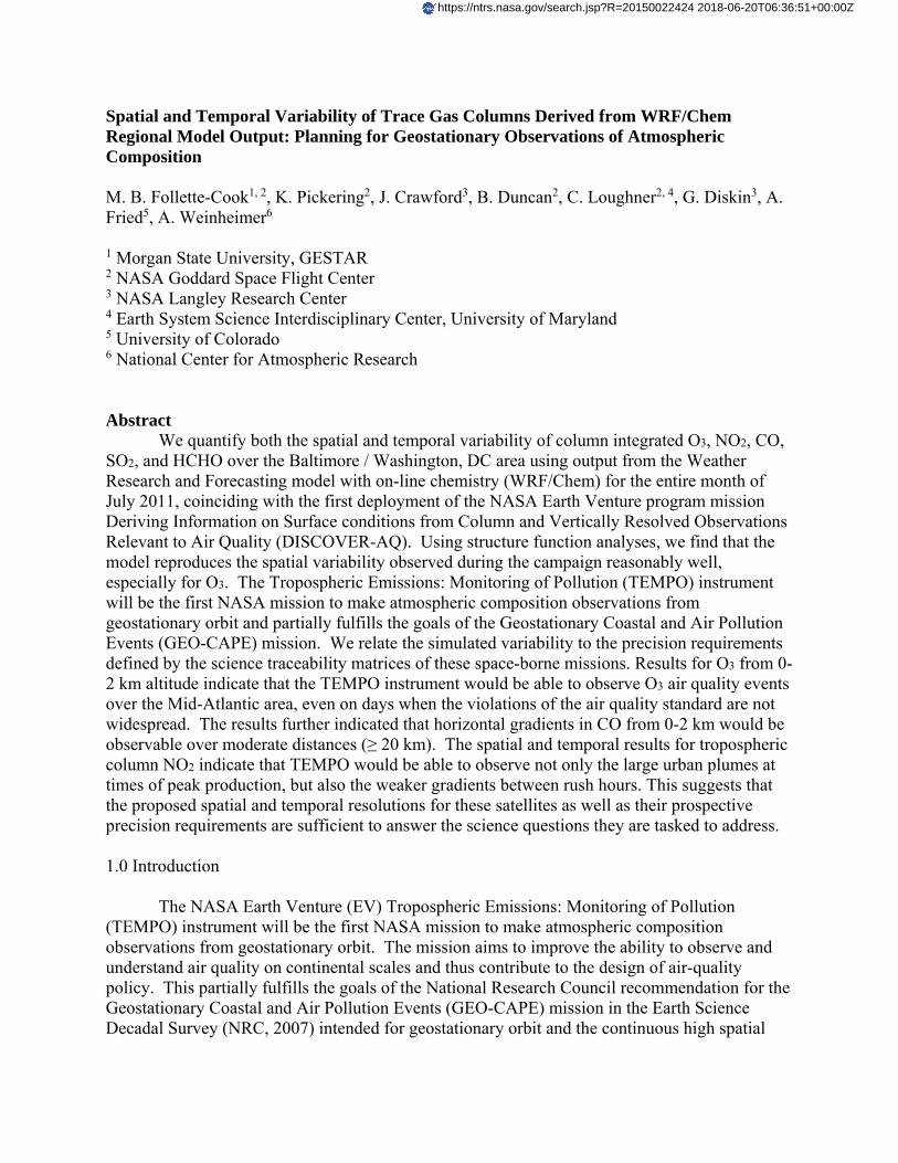
Spatial and Temporal Variability of Trace Gas Columns Derived from WRF/Chem Regional Model Output: Planning for Geostationary Observations of Atmospheric Composition M. B. Follette-Cook1, 2, K. Pickering2, J. Crawford3, B. Duncan2, C. Loughner2, 4, G. Diskin3, A. Fried5, A. Weinheimer6 1 Morgan State University, GESTAR 2 NASA Goddard Space Flight Center 3 NASA Langley Research Center 4 Earth System Science Interdisciplinary Center, University of Maryland 5 University of Colorado 6 National Center for Atmospheric Research Abstract

We quantify both the spatial and temporal variability of column integrated O3, NO2, CO, SO2, and HCHO over the Baltimore / Washington, DC area using output from the Weather Research and Forecasting model with on-line chemistry (WRF/Chem) for the entire month of July 2011, coinciding with the first deployment of the NASA Earth Venture program mission Deriving Information on Surface conditions from Column and Vertically Resolved Observations Relevant to Air Quality (DISCOVER-AQ). Using structure function analyses, we find that the model reproduces the spatial variability observed during the campaign reasonably well, especially for O3. The Tropospheric Emissions: Monitoring of Pollution (TEMPO) instrument will be the first NASA mission to make atmospheric composition observations from geostationary orbit and partially fulfills the goals of the Geostationary Coastal and Air Pollution Events (GEO-CAPE) mission. We relate the simulated variability to the precision requirements defined by the science traceability matrices of these space-borne missions. Results for O3 from 0-2 km altitude indicate that the TEMPO instrument would be able to observe O3 air quality events over the Mid-Atlantic area, even on days when the violations of the air quality standard are not widespread. The results further indicated that horizontal gradients in CO from 0-2 km would be observable over moderate distances (≥ 20 km). The spatial and temporal results for tropospheric column NO2 indicate that TEMPO would be able to observe not only the large urban plumes at times of peak production, but also the weaker gradients between rush hours. This suggests that the proposed spatial and temporal resolutions for these satellites as well as their prospective precision requirements are sufficient to answer the science questions they are tasked to address. 1.0 Introduction

The NASA Earth Venture (EV) Tropospheric Emissions: Monitoring of Pollution

(TEMPO) instrument will be the first NASA mission to make atmospheric composition observations from geostationary orbit. The mission aims to improve the ability to observe and understand air quality on continental scales and thus contribute to the design of air-quality policy. This partially fulfills the goals of the National Research Council recommendation for the Geostationary Coastal and Air Pollution Events (GEO-CAPE) mission in the Earth Science Decadal Survey (NRC, 2007) intended for geostationary orbit and the continuous high spatial

https://ntrs.nasa.gov/search.jsp?R=20150022424 2018-06-20T06:36:51+00:00Z

and temporal resolution measurements it can uniquely provide. TEMPO is a UV/VIS spectrometer that will provide high resolution daylight measurements of O3, NO2, HCHO, SO2, glyoxal (OCHCHO), water vapor, and aerosols (Chance et al., 2013). Set to launch in late 2018 on a hosted platform, this instrument will provide measurements at a spatial resolution of 8.4 x 4.5 km at the center of the domain. HCHO, SO2, and glyoxal products will be measured three times a day, while observations of O3 and NO2 will be made hourly. TEMPO fulfills the UV/VIS component of GEO-CAPE, which additionally calls for hourly measurements of CO. TEMPO will be part of a three-satellite constellation in geostationary orbit. The Geostationary Environment Monitoring Spectrometer (GEMS) will observe the Asia-Pacific region (Kim et al. 2012), and is scheduled to launch in 2018. In 2019, Sentinel-4 will begin to observe Europe and northern Africa (Bovensman et al., 2002; Burrows et al., 2004; Bovensman et al., 2004).

One of the main objectives of both TEMPO and GEO-CAPE is to address the science question, “What are the temporal and spatial variations of emissions of gases and aerosols important for air quality and climate?” (Fishman et al. 2012). That work also states that the instruments, “… must be designed to capture the portion of this variability that is important for describing the emission, chemistry, and transport of gases and aerosols … providing information to the air quality community at spatial and temporal scales relevant for analysis of high-emission corridors within urban areas, the photochemical cycles involving nonmethane hydrocarbons, nitrogen oxides (NOx), and O3, and the variability induced by mesoscale meteorological phenomena (e.g., land/sea breezes).”

Variability in atmospheric composition exists at every scale. The spatial and temporal variability of a trace gas will be determined by the chemistry of the species, the spatial and temporal patterns of emissions, and the spatial scales over which a species will experience transport during its lifetime. Given the proposed spatial and temporal resolutions and the mission precision requirements, what kind of variability will these geostationary instruments have the capability to observe? Previously, Loughner et al. (2007) used variograms, calculated using model-generated fields, to determine the length scales of ozone variability as a function of altitude. They found that ozone was most variable (i.e., had the shortest length scales) near the surface in the planetary boundary layer (PBL) and this variability was reflected in the similar length scales of the tropospheric column. Fishman et al. (2011) also used model-generated fields to conduct a detailed analysis relating the variability of O3, NO2, and CO over the Houston, TX area to satellite observing requirements. Model results indicated that variability in the planetary boundary layer (PBL) drove the variability of the tropospheric column for O3, CO, and NO2. Both of these previous studies focused on the spatial variability of trace gases. In this work, we quantify both the spatial and temporal variability of O3, NO2, CO, SO2, and HCHO over the Baltimore / Washington, DC area for the entire month of July 2011 using output from the Weather Research and Forecasting model with on-line chemistry (WRF/Chem) (Grell et al. 2005). We then relate the simulated variability to the precision requirements of the proposed instruments. This time period coincides with the first deployment of the NASA Earth Venture (EV) program mission, Deriving Information on Surface conditions from Column and Vertically Resolved Observations Relevant to Air Quality (DISCOVER-AQ).

Section 2 of this work describes the DISCOVER-AQ observations used to compare with the model results. Section 3 outlines the WRF/Chem simulation. In Section 4 we compare the model output variability with observations. Sections 5 and 6 contain the horizontal and temporal analyses, respectively. Conclusions are stated in Section 7.

2.0 Observations

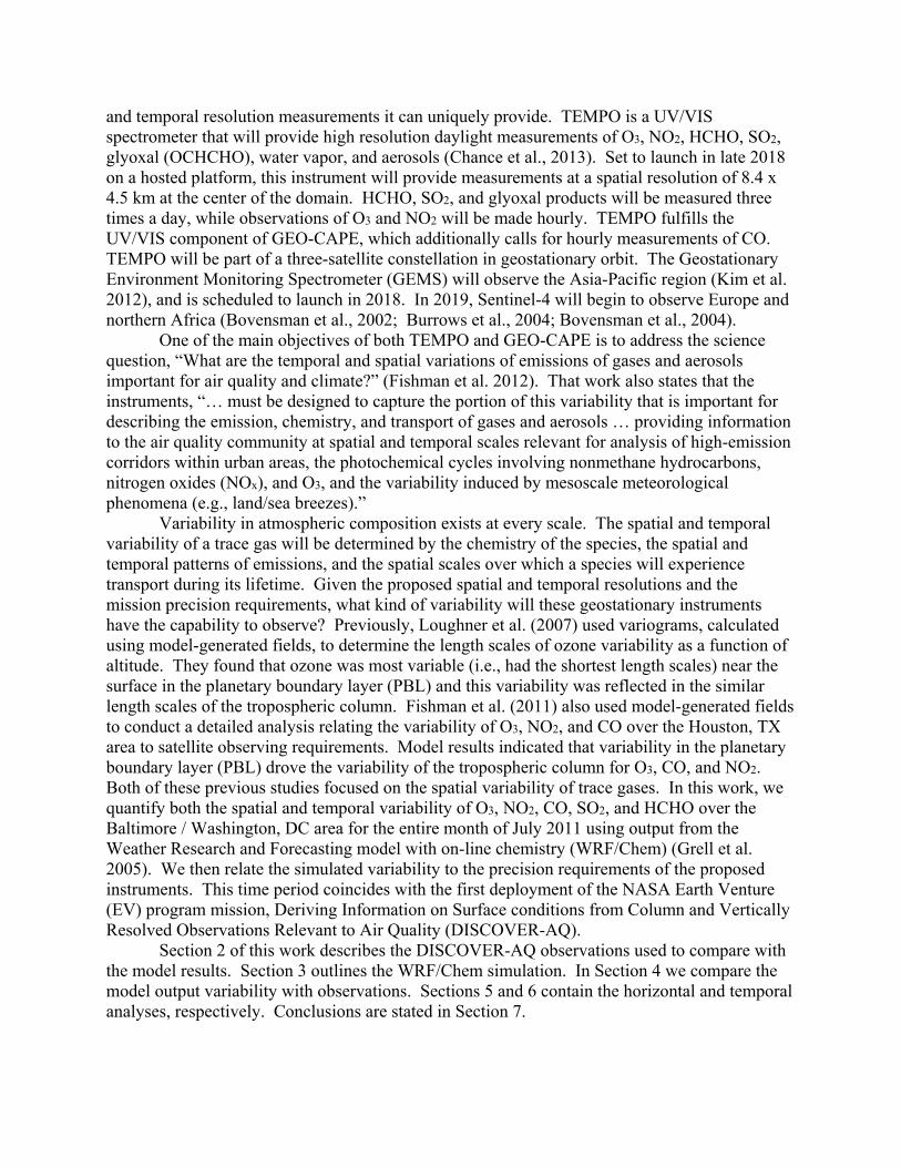
Before examining variability within the model simulation, we first evaluate the model output against in-situ measurements made over the Baltimore / Washington, DC area (BWA) during the July 2011 deployment of DISCOVER-AQ. The main goal of DISCOVER-AQ is to characterize the relationship between air quality at the surface and in the tropospheric columns that can be measured from a satellite. This is accomplished with an observing strategy that includes concurrent in situ and remote sensing observations from a network of ground sites and two research aircraft. A graphic of the platforms, measurement methods, and P-3B flight path is shown in Figure 1. The P-3B aircraft carried in-situ instruments and made three circuits of the flight path each flight day. The payload of the King Air B200 aircraft included a UV/VIS remote sensing instrument for trace gases and an aerosol lidar. The B200 made two sorties on each flight day (flight path not shown) with a stop in between for refueling. P-3B flights typically lasted about eight hours, allowing for the observation of diurnal variability (data: doi:10.5067/Aircraft/DISCOVER-AQ/Aerosol-TraceGas or http://www-air.larc.nasa.gov/missions/discover-aq/discover-aq.html).

The variety of meteorological flight conditions, air quality conditions, consistent flight patterns, and large sample size make the DISCOVER-AQ dataset ideal for evaluating the ability of the model to reproduce variability. Fourteen science flights were conducted between July 1 and July 29, 2011. July 2011 is the fourth warmest July on record for the U.S., and the warmest July for the Baltimore area with respect to monthly mean maximum temperatures. Baltimore Washington International (BWI) Thurgood Marshall Airport near Baltimore, MD recorded 24 days with temperatures ≥ 90F.

Over the course of the month, the BWA experienced three weather “regimes”. The beginning of the month was characterized by high temperatures (BWI recorded nine days out of 13 with maximum temperatures ≥ 90F) and several high pressure systems. A Canadian air mass

Figure 1. Graphic overview of the platforms, measurement methods, and P-3B flight path for the BWA deployment of DISCOVER-AQ (credit: Timothy Marvel).

moved into the region on July 14, leading to very clean conditions with lower RH (mean dew points < 65 F and RH < 64%). On July 20, intense heat from the Midwest associated with an upper level ridge started to move over the northeast corridor of the U.S., stretching from Washington, DC to Boston, MA. This heat wave event peaked on July 22 when BWI Airport reached 105 °F (41 °C), and downtown Baltimore, MD reached 107 °F (42 °C). The heat wave was characterized by high RH, high minimum overnight temperatures, and poor air quality. A frontal system passed through the region on July 25, lowering dew points considerably and daytime temperatures slightly. By July 28, higher dew points and temperatures dominated through the end of the mission on July 29. During July 2011, there were three days in which O3 monitoring stations in Maryland recorded 8-hr O3 values that were between 95 and 115 ppbv (or “code red,” U.S. EPA, 2009), and 13 days with 8-hr O3 values between 76 and 95 ppbv (or “code orange”). Eight-hour O3 values greater than 75 ppbv are violations of the current EPA standard for O3 (U.S. EPA, 2011). DISCOVER-AQ conducted flights on all three code red days, and seven out of the 13 code orange days. 3.0 WRF/Chem Simulation

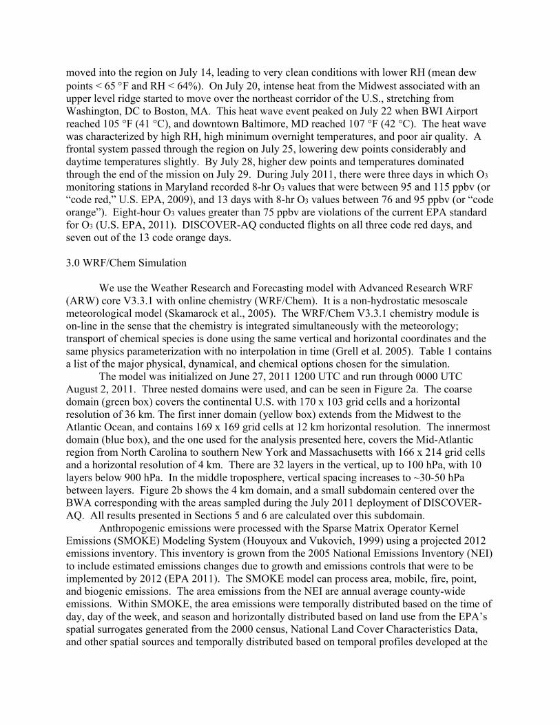
We use the Weather Research and Forecasting model with Advanced Research WRF (ARW) core V3.3.1 with online chemistry (WRF/Chem). It is a non-hydrostatic mesoscale meteorological model (Skamarock et al., 2005). The WRF/Chem V3.3.1 chemistry module is on-line in the sense that the chemistry is integrated simultaneously with the meteorology; transport of chemical species is done using the same vertical and horizontal coordinates and the same physics parameterization with no interpolation in time (Grell et al. 2005). Table 1 contains a list of the major physical, dynamical, and chemical options chosen for the simulation. The model was initialized on June 27, 2011 1200 UTC and run through 0000 UTC August 2, 2011. Three nested domains were used, and can be seen in Figure 2a. The coarse domain (green box) covers the continental U.S. with 170 x 103 grid cells and a horizontal resolution of 36 km. The first inner domain (yellow box) extends from the Midwest to the Atlantic Ocean, and contains 169 x 169 grid cells at 12 km horizontal resolution. The innermost domain (blue box), and the one used for the analysis presented here, covers the Mid-Atlantic region from North Carolina to southern New York and Massachusetts with 166 x 214 grid cells and a horizontal resolution of 4 km. There are 32 layers in the vertical, up to 100 hPa, with 10 layers below 900 hPa. In the middle troposphere, vertical spacing increases to ~30-50 hPa between layers. Figure 2b shows the 4 km domain, and a small subdomain centered over the BWA corresponding with the areas sampled during the July 2011 deployment of DISCOVER-AQ. All results presented in Sections 5 and 6 are calculated over this subdomain. Anthropogenic emissions were processed with the Sparse Matrix Operator Kernel Emissions (SMOKE) Modeling System (Houyoux and Vukovich, 1999) using a projected 2012 emissions inventory. This inventory is grown from the 2005 National Emissions Inventory (NEI) to include estimated emissions changes due to growth and emissions controls that were to be implemented by 2012 (EPA 2011). The SMOKE model can process area, mobile, fire, point, and biogenic emissions. The area emissions from the NEI are annual average county-wide emissions. Within SMOKE, the area emissions were temporally distributed based on the time of day, day of the week, and season and horizontally distributed based on land use from the EPA’s spatial surrogates generated from the 2000 census, National Land Cover Characteristics Data, and other spatial sources and temporally distributed based on temporal profiles developed at the

EPA. Point source emissions were vertically distributed based on meteorology, stack height, and temperature and velocity of the emissions. Mobile emissions were processed with the Motor Vehicle Emission Simulator (MOVES; US EPA 2012). Biomass burning emissions were obtained from the Fire Inventory from NCAR version 1.0 (FINNv1; Wiedinmyer et al. 2011) and were vertically distributed based on a plume rise algorithm within the WRF/Chem modeling system. Biogenic emissions were calculated within WRF/Chem using the Model of Emissions of Gases and Aerosols from Nature (MEGAN v2; Guenther et al., 2012). Meteorological initial and boundary conditions were taken from North American Regional Reanalysis (NARR) dataset. Chemical initial and boundary conditions were generated

Figure 2. a) Three domains used for the WRF/Chem simulation, 36 km (green box), 12 km (yellow box), and 4 km (blue box). b) 4 km domain (blue) and subdomain used for structure function calculations (red)

Table 1. WRF-Chem Model Configuration Used for This Studya

at 6-hour time intervals by the MOZART-4 global chemical transport model (Emmons et al. 2010). Objective analysis (OBSGRID) nudging was used to improve the mesoscale grid by incorporating information from observations. For this analysis, high resolution upper level and surface observations were combined with the global analysis fields (Yegorova et al. 2011). In addition, Four-Dimensional Data Assimilation (FDDA) nudging was used. Temperature, water vapor, and winds were nudged towards analysis fields for the coarse domain. 4.0 WRF/Chem and DISCOVER-AQ Variability

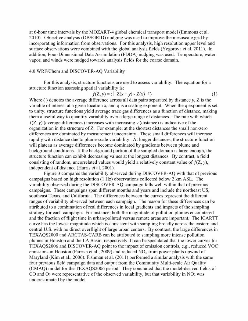
For this analysis, structure functions are used to assess variability. The equation for a structure function assessing spatial variability is: (Z, y) Z(x + y) - Z(x)q (1) Where denotes the average difference across all data pairs separated by distance y, Z is the variable of interest at a given location x, and q is a scaling exponent. When the q exponent is set to unity, structure functions yield average trace gas differences as a function of distance, making them a useful way to quantify variability over a large range of distances. The rate with which (Z, y) (average differences) increases with increasing y (distance) is indicative of the organization in the structure of Z. For example, at the shortest distances the small non-zero differences are dominated by measurement uncertainty. These small differences will increase rapidly with distance due to plume-scale variability. At longer distances, the structure function will plateau as average differences become dominated by gradients between plume and background conditions. If the background portion of the sampled domain is large enough, the structure function can exhibit decreasing values at the longest distances. By contrast, a field consisting of random, uncorrelated values would yield a relatively constant value of (Z, y), independent of distance (Harris et al. 2001). Figure 3 compares the variability observed during DISCOVER-AQ with that of previous campaigns based on high resolution (1 Hz) observations collected below 2 km ASL. The variability observed during the DISCOVER-AQ campaign falls well within that of previous campaigns. These campaigns span different months and years and include the northeast US, southeast Texas, and California. The differences between the curves represent the different ranges of variability observed between each campaign. The reason for these differences can be attributed to a combination of real differences in local gradients and impacts of the sampling strategy for each campaign. For instance, both the magnitude of pollution plumes encountered and the fraction of flight time in urban/polluted versus remote areas are important. The ICARTT curve has the lowest magnitude which is consistent with sampling broadly across the eastern and central U.S. with no direct overflight of large urban centers. By contrast, the large differences in TEXAQS2000 and ARCTAS-CARB can be attributed to sampling more intense pollution plumes in Houston and the LA Basin, respectively. It can be speculated that the lower curves for TEXAQS2006 and DISCOVER-AQ point to the impact of emission controls, e.g., reduced VOC emissions in Houston (Parrish et al., 2009) and reduced NOx from power plants upwind of Maryland (Kim et al., 2006). Fishman et al. (2011) performed a similar analysis with the same four previous field campaign data and output from the Community Multi-scale Air Quality (CMAQ) model for the TEXAQS2006 period. They concluded that the model-derived fields of CO and O3 were representative of the observed variability, but that variability in NO2 was underestimated by the model.

We evaluate the variability simulated by the model by comparing structure functions of

O3, NO2, CO, and HCHO calculated using the WRF/Chem output with structure functions based on the DISCOVER-AQ observations (Figure 4). For this analysis, the WRF/Chem output was collocated in space and time with a 1-second merge of the P-3B data. However, the additional statistics shown in Figure 4a go beyond the simple average presented in equation 1. Here, percentile statistics for the full distribution of differences at each binned distance is provided. These plots summarize the point-to-point differences observed during the entire campaign. Figure 4b shows the P-3B-WRF/Chem difference for each percentile.

Overall, WRF/Chem captures the shapes of the variability curves, and reproduces the observed variability in O3 particularly well. WRF/Chem slightly overestimates 95th percentile O3 variability by ~2 ppbv at distances <12 km. This increases to ~5 ppbv at distances >12km. The variability in CO and NO2 are also overestimated by the model, and like O3, that overestimation increases with increasing distance. The largest overestimation occurs for the highest percentiles, indicating that the urban-to-background gradient is likely too large in the model. It should be noted that the maximum differences in NO2 (not shown) at all distances and maximum differences in CO at distances >16 km show a 30 ppbv, and 0-50ppbv underestimation by WRF/Chem, respectively. HCHO 95th percentile variability is consistently underestimated by ~2 ppbv at all distances.

In order to evaluate the ability of the model to simulate temporal changes, the collocated WRF/Chem output described above and the DISCOVER-AQ observations were used to calculate averages centered on the hour for the entire campaign. Structure functions could not be used to compare with the aircraft data given the lack of temporal continuity at a given location Figure 5 shows the WRF/Chem and P-3B averages for O3, NO2, CO, and HCHO. All data points that were below 2 km and fell within 15 minutes of the hour were included. Similar to the results shown in Figure 4, the comparison of O3 yields the best results. The model slightly overestimates NO2 beginning at 11 am, and overestimates CO at all hours before 6 pm EDT. The underestimation of HCHO by the model seen in the spatial structure functions in Figure 4 is also seen in the hourly averages. The model does well until 11 am EDT, after which it largely underestimates HCHO.

Figure 3. Structure functions for a) O3 and b) NO2 calculated using data from the June 2008 Arctic Research

of the Composition of the Troposphere from Aircraft and Satellites - California Air Resources Board (ARCTAS-CARB: blue), the Jul – Aug 2004 International Consortium for Atmospheric Research on Transport and Transformation (ICARTT: light blue), the Texas Air Quality Study in Aug – Sep 2000 (TEXAQS2000: green) and Aug – Sep 2006 (TEXAQS2006: red) campaigns, and the July 2011 DISCOVER-AQ campaign (black).

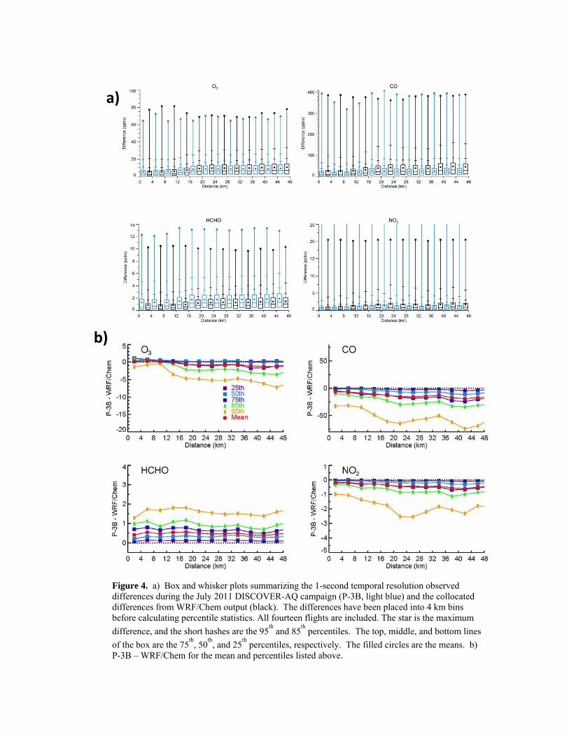
Figure 4. a) Box and whisker plots summarizing the 1-second temporal resolution observed differences during the July 2011 DISCOVER-AQ campaign (P-3B, light blue) and the collocated differences from WRF/Chem output (black). The differences have been placed into 4 km bins before calculating percentile statistics. All fourteen flights are included. The star is the maximum

difference, and the short hashes are the 95th and 85

th percentiles. The top, middle, and bottom lines

of the box are the 75th

, 50th

, and 25th

percentiles, respectively. The filled circles are the means. b) P-3B – WRF/Chem for the mean and percentiles listed above.

a)

b)

The overestimation of CO and NO2 could be the result of the emissions used. Anderson

et al. (2014) evaluated the NEI emissions database for the BWA using in-situ observations made during the DISCOVER-AQ campaign. Observation-based emissions ratios and mixing ratios of CO/NOx were compared with output from the Community Multi-scale Air Quality (CMAQ) model. They concluded that the NEI database overestimates NOx (NOx = NO + NO2) emissions by 75 ± 24%, and that the mobile NOx emissions were the primary source of error. They also calculated an overestimation of CO of 15 ± 11%.

The underestimation of HCHO is most likely due to missing source species or missing primary emissions of HCHO. A major VOC source for HCHO in the BWA is the oxidation of isoprene (Trainer et al., 2000); however there is no corresponding underestimation of isoprene (not shown).

5.0 Spatial Variability

As stated in the introduction, the purpose of quantifying variability is to gauge how much

of that variability would be observable by the geostationary platforms in question. TEMPO will provide observations at high spatial resolution, ~4 x ~8 km. To incorporate instrument plans into our analysis, we use the prospective precision requirements (PR) for each trace gas of interest (Table 2). The PR for CO comes from the GEO-CAPE science traceability matrix (STM) (Fishman et al., 2012), and the remaining trace gas PR (O3, NO2, HCHO, and SO2) come from the TEMPO STM (Chance et al., 2013). The PRs for O3 and CO are listed in terms of mixing

Figure 5. Hourly averaged O3, CO, HCHO, and NO2 calculated using

DISCOVER-AQ P-3B measurements (light blue) and collocated WRF/Chem output (black). All fourteen flights are included.

ratio for specific altitude ranges, 0 – 2 km (referred to hereafter as the boundary layer, or BL), 2 km – tropopause (referred to hereafter as the free troposphere, or FT), or tropospheric column. WRF/Chem, as configured for this analysis, does not have a stratosphere, so for our analysis we use 200 hPa as our upper limit for the troposphere (i.e. the tropopause). For these species, the corresponding columns are calculated by taking the PR and integrating over the altitude range (see Table 2). The PRs for NO2, SO2, and HCHO are given in terms of column abundances. To examine the variability over the BWA for July 2011, a small subdomain was chosen to correspond with the geographic coverage of DISCOVER-AQ. This subdomain consisted of 1002 grid cells and can be seen in Figure 2b (red box). Three column quantities were calculated for O3 and CO: 0 – 2 km, 2 km – tropopause, and tropospheric columns. There is no PR for FT O3 but we have shown the results for completeness. Only tropospheric columns were computed for NO2, HCHO, and SO2. Similar to Figure 4a, Figure 6 shows the percentile statistics for the full distribution of differences at each binned distance based on differences across the model subdomain for every day of July 2011 at 6 different hours, 12, 14, 16, 18, 20, and 22 UTC (corresponding to 8 am, 10 am, 12 pm, 2 pm, 4 pm, and 6 pm EDT). The dotted black line on each plot is the precision requirement for that species. Points that fall below the PR are differences that would, hypothetically, be too small to detect.

The interpretation of these plots is best explained by first considering a single species, e.g. tropospheric column NO2. For all days of July 2011, and for the six hours specified above, at distances between 4 and 8 km, the median difference between NO2 data pairs was ~0.3x1015

Table 2. TEMPO (O3, NO2, HCHO, and SO2) and GEO-CAPE (CO) Precision Requirements

* Column quantities for O3 and CO were calculated using the precision requirement value in terms of mixing ratio

and integrating over the altitude range specified. 1 (Kelly Chance, personal communication)

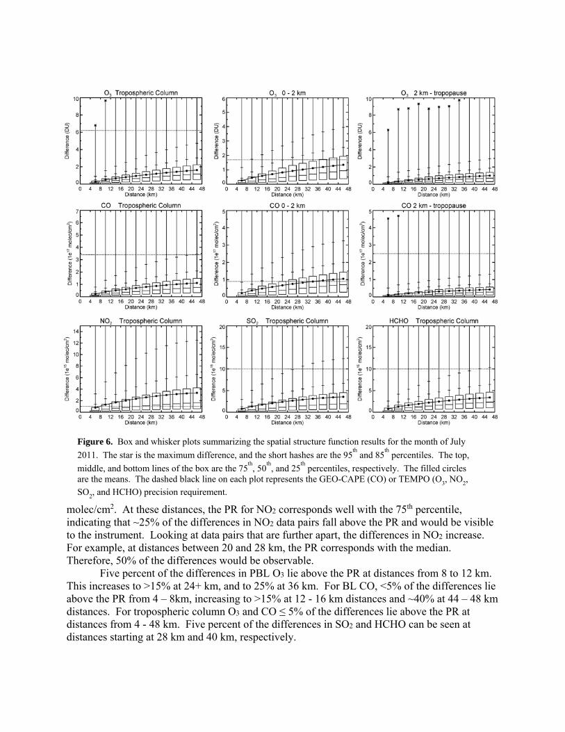
molec/cm2. At these distances, the PR for NO2 corresponds well with the 75th percentile, indicating that ~25% of the differences in NO2 data pairs fall above the PR and would be visible to the instrument. Looking at data pairs that are further apart, the differences in NO2 increase. For example, at distances between 20 and 28 km, the PR corresponds with the median. Therefore, 50% of the differences would be observable.

Five percent of the differences in PBL O3 lie above the PR at distances from 8 to 12 km. This increases to >15% at 24+ km, and to 25% at 36 km. For BL CO, <5% of the differences lie above the PR from 4 – 8km, increasing to >15% at 12 - 16 km distances and ~40% at 44 – 48 km distances. For tropospheric column O3 and CO ≤ 5% of the differences lie above the PR at distances from 4 - 48 km. Five percent of the differences in SO2 and HCHO can be seen at distances starting at 28 km and 40 km, respectively.

Figure 6. Box and whisker plots summarizing the spatial structure function results for the month of July

2011. The star is the maximum difference, and the short hashes are the 95th and 85

th percentiles. The top,

middle, and bottom lines of the box are the 75th

, 50th

, and 25th

percentiles, respectively. The filled circles are the means. The dashed black line on each plot represents the GEO-CAPE (CO) or TEMPO (O3, NO2,

SO2, and HCHO) precision requirement.

These results might appear as though the PRs are inadequate for answering the proposed science questions, but some specification and context is needed. First, these plots only address spatial variability probability in the evaluated scene across the entire month. Differences in time are equally important, such as between days (e.g., clean versus polluted) or time of day (morning versus afternoon). Ozone for example, tends to increase and decrease regionally and can be expected to exhibit larger differences from day-to-day than spatially across a local area. In addition, larger spatial differences are more likely in the afternoon due to the photochemical production of O3 throughout the day. Lumping clean days with polluted days also prevents a clear assessment of spatial variability during a pollution episode when satellite observations would be most valuable. A discussion of each of these issues will be presented below. 5.1 Monthly variability

We will first address the range of variability quantified for each day within the model output. One might expect clean days to be more homogeneous than polluted days, such that large spatial differences are weighted more heavily to polluted days. To examine this, the percentage of differences greater than the PR were determined for each distance bin (e.g. 4 – 8 km), for every hourly scene. This percentage is hereafter referred to as the “Percent Above PR”, or PAPR). Figure 7 shows the range of those percentages over the course of July 2011, and includes all six hours of each day. These ranges are summarized in box and whisker plots where the top, middle, and bottom of the box are the 75th, 50th (median), and 25th percentiles, respectively. The vertical line extends from the minimum to the maximum, and the circles are the means. Taking tropospheric column NO2 as an example again, at distances between 4 and 8 km the mean percentage that fell above the PR is 21%, but the range extends from 7 to 48%. Starting at 28 km distances, there are times when 80% of the differences would be detected. Overall, Figure 7 shows that each species has a considerable range of PAPR values, corresponding with the range of variability seen over the course of the month.

At distances between 8 and 12 km, the PBL O3 PAPR ranges from 0 to 25% with a mean of <5%. The range increases rapidly, and starting at distances of 20 km, there are hours where the PAPR is > 50%. Greater variability is seen in PBL CO. At distances between 4 and 8 km, the PAPR ranges from <1 to 20% with a mean of 4%, and > 50% of the differences fall above the PR at some hours starting at 16 km distances. These results indicate that at certain times, > 50% of the spatial differences in BL O3 and CO will be observable over moderate distances (≥ 16-20 km).

The mean PAPR for tropospheric O3 ranges from <1 – 1.7%, and the maximum PAPR is over 20% starting at 36 km distances. The mean PAPR increases from <1% to 5.2%, from 4 - 48 km, for tropospheric column CO, and is <1% for FT CO. The results for SO2 and HCHO show that the mean PAPRs range from <1 – 7.7% and from <1 – 5.6%, respectively.

5.2 Hourly variability As stated above, the variability of some species has a diurnal cycle, leading to larger percentages of differences that lie above the PR at particular daylight hours. Figure 8 shows the mean PAPR for the month of July 2011, for the six individual hours analyzed (12, 14, 16, 18, 20 and 22 UTC). These curves were generated by taking the mean of all of the PAPR values at each individual hour. Tropospheric column O3 shows the largest mean PAPR values, i.e. the largest differences or greatest variability, after 2 pm EDT (18 UTC). Ozone in the PBL shows the largest values at 2 pm and 4 pm (20 UTC), and slightly lower values at 6 pm (22 UTC). These

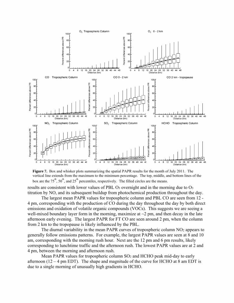
results are consistent with lower values of PBL O3 overnight and in the morning due to O3 titration by NO, and its subsequent buildup from photochemical production throughout the day. The largest mean PAPR values for tropospheric column and PBL CO are seen from 12 - 4 pm, corresponding with the production of CO during the day throughout the day by both direct emissions and oxidation of volatile organic compounds (VOCs). This suggests we are seeing a well-mixed boundary layer form in the morning, maximize at ~2 pm, and then decay in the late afternoon early evening. The largest PAPR for FT CO are seen around 2 pm, when the column from 2 km to the tropopause is likely influenced by the PBL.

The diurnal variability in the mean PAPR curves of tropospheric column NO2 appears to generally follow emissions patterns. For example, the largest PAPR values are seen at 8 and 10 am, corresponding with the morning rush hour. Next are the 12 pm and 6 pm results, likely corresponding to lunchtime traffic and the afternoon rush. The lowest PAPR values are at 2 and 4 pm, between the morning and afternoon rush.

Mean PAPR values for tropospheric column SO2 and HCHO peak mid-day to early afternoon (12 – 4 pm EDT). The shape and magnitude of the curve for HCHO at 8 am EDT is due to a single morning of unusually high gradients in HCHO.

Figure 7. Box and whisker plots summarizing the spatial PAPR results for the month of July 2011. The vertical line extends from the maximum to the minimum percentage. The top, middle, and bottom lines of the

box are the 75th, 50

th, and 25

th percentiles, respectively. The filled circles are the means.

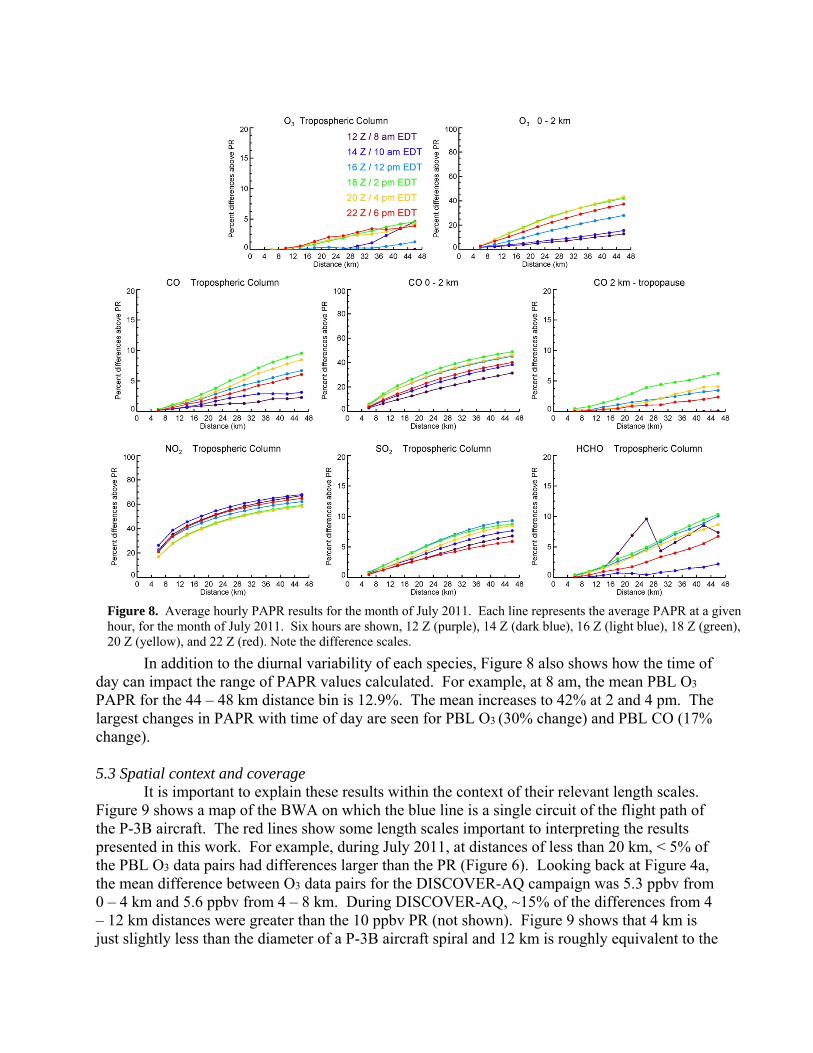
In addition to the diurnal variability of each species, Figure 8 also shows how the time of day can impact the range of PAPR values calculated. For example, at 8 am, the mean PBL O3 PAPR for the 44 – 48 km distance bin is 12.9%. The mean increases to 42% at 2 and 4 pm. The largest changes in PAPR with time of day are seen for PBL O3 (30% change) and PBL CO (17% change).

5.3 Spatial context and coverage It is important to explain these results within the context of their relevant length scales. Figure 9 shows a map of the BWA on which the blue line is a single circuit of the flight path of the P-3B aircraft. The red lines show some length scales important to interpreting the results presented in this work. For example, during July 2011, at distances of less than 20 km, < 5% of the PBL O3 data pairs had differences larger than the PR (Figure 6). Looking back at Figure 4a, the mean difference between O3 data pairs for the DISCOVER-AQ campaign was 5.3 ppbv from 0 – 4 km and 5.6 ppbv from 4 – 8 km. During DISCOVER-AQ, ~15% of the differences from 4 – 12 km distances were greater than the 10 ppbv PR (not shown). Figure 9 shows that 4 km is just slightly less than the diameter of a P-3B aircraft spiral and 12 km is roughly equivalent to the

Figure 8. Average hourly PAPR results for the month of July 2011. Each line represents the average PAPR at a given hour, for the month of July 2011. Six hours are shown, 12 Z (purple), 14 Z (dark blue), 16 Z (light blue), 18 Z (green), 20 Z (yellow), and 22 Z (red). Note the difference scales.

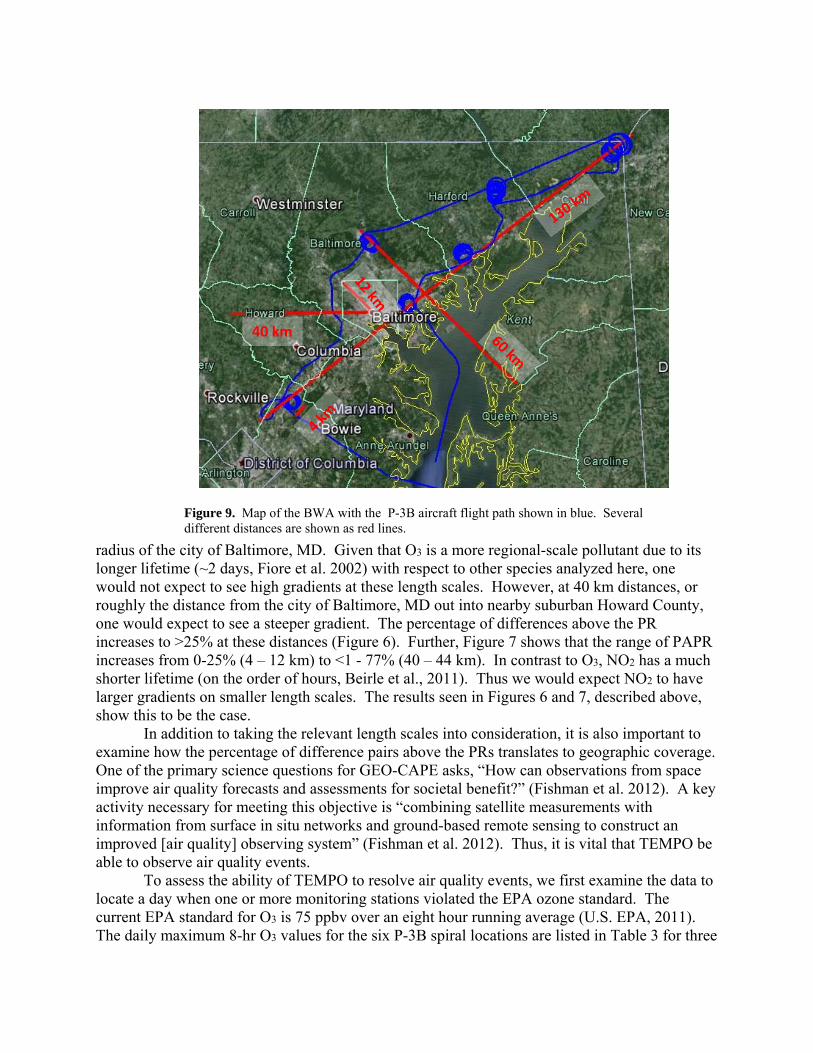
radius of the city of Baltimore, MD. Given that O3 is a more regional-scale pollutant due to its longer lifetime (~2 days, Fiore et al. 2002) with respect to other species analyzed here, one would not expect to see high gradients at these length scales. However, at 40 km distances, or roughly the distance from the city of Baltimore, MD out into nearby suburban Howard County, one would expect to see a steeper gradient. The percentage of differences above the PR increases to >25% at these distances (Figure 6). Further, Figure 7 shows that the range of PAPR increases from 0-25% (4 – 12 km) to <1 - 77% (40 – 44 km). In contrast to O3, NO2 has a much shorter lifetime (on the order of hours, Beirle et al., 2011). Thus we would expect NO2 to have larger gradients on smaller length scales. The results seen in Figures 6 and 7, described above, show this to be the case.

In addition to taking the relevant length scales into consideration, it is also important to examine how the percentage of difference pairs above the PRs translates to geographic coverage. One of the primary science questions for GEO-CAPE asks, “How can observations from space improve air quality forecasts and assessments for societal benefit?” (Fishman et al. 2012). A key activity necessary for meeting this objective is “combining satellite measurements with information from surface in situ networks and ground-based remote sensing to construct an improved [air quality] observing system” (Fishman et al. 2012). Thus, it is vital that TEMPO be able to observe air quality events.

To assess the ability of TEMPO to resolve air quality events, we first examine the data to locate a day when one or more monitoring stations violated the EPA ozone standard. The current EPA standard for O3 is 75 ppbv over an eight hour running average (U.S. EPA, 2011). The daily maximum 8-hr O3 values for the six P-3B spiral locations are listed in Table 3 for three

40 km

Figure 9. Map of the BWA with the P-3B aircraft flight path shown in blue. Several different distances are shown as red lines.

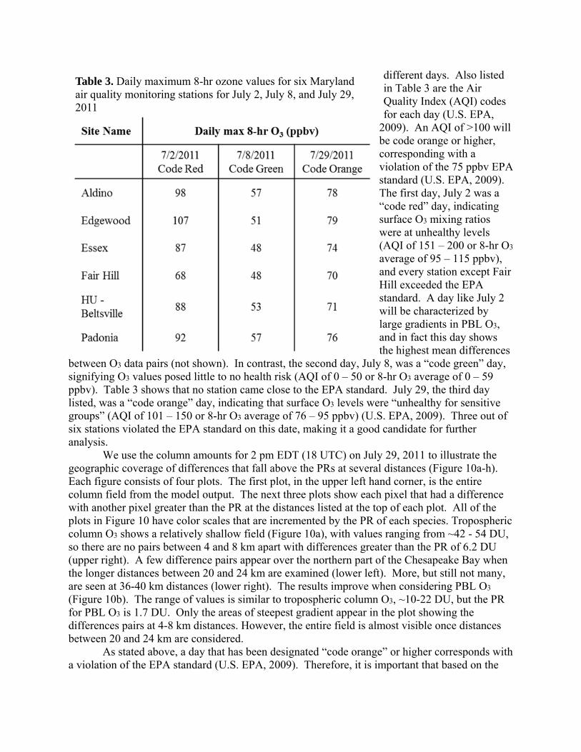
different days. Also listed in Table 3 are the Air Quality Index (AQI) codes for each day (U.S. EPA,

2009). An AQI of >100 will be code orange or higher, corresponding with a violation of the 75 ppbv EPA standard (U.S. EPA, 2009). The first day, July 2 was a “code red” day, indicating surface O3 mixing ratios were at unhealthy levels (AQI of 151 – 200 or 8-hr O3 average of 95 – 115 ppbv), and every station except Fair Hill exceeded the EPA standard. A day like July 2 will be characterized by large gradients in PBL O3, and in fact this day shows the highest mean differences

between O3 data pairs (not shown). In contrast, the second day, July 8, was a “code green” day, signifying O3 values posed little to no health risk (AQI of 0 – 50 or 8-hr O3 average of 0 – 59 ppbv). Table 3 shows that no station came close to the EPA standard. July 29, the third day listed, was a “code orange” day, indicating that surface O3 levels were “unhealthy for sensitive groups” (AQI of 101 – 150 or 8-hr O3 average of 76 – 95 ppbv) (U.S. EPA, 2009). Three out of six stations violated the EPA standard on this date, making it a good candidate for further analysis.

We use the column amounts for 2 pm EDT (18 UTC) on July 29, 2011 to illustrate the geographic coverage of differences that fall above the PRs at several distances (Figure 10a-h). Each figure consists of four plots. The first plot, in the upper left hand corner, is the entire column field from the model output. The next three plots show each pixel that had a difference with another pixel greater than the PR at the distances listed at the top of each plot. All of the plots in Figure 10 have color scales that are incremented by the PR of each species. Tropospheric column O3 shows a relatively shallow field (Figure 10a), with values ranging from ~42 - 54 DU, so there are no pairs between 4 and 8 km apart with differences greater than the PR of 6.2 DU (upper right). A few difference pairs appear over the northern part of the Chesapeake Bay when the longer distances between 20 and 24 km are examined (lower left). More, but still not many, are seen at 36-40 km distances (lower right). The results improve when considering PBL O3

(Figure 10b). The range of values is similar to tropospheric column O3, ~10-22 DU, but the PR for PBL O3 is 1.7 DU. Only the areas of steepest gradient appear in the plot showing the differences pairs at 4-8 km distances. However, the entire field is almost visible once distances between 20 and 24 km are considered.

As stated above, a day that has been designated “code orange” or higher corresponds with a violation of the EPA standard (U.S. EPA, 2009). Therefore, it is important that based on the

Table 3. Daily maximum 8-hr ozone values for six Maryland air quality monitoring stations for July 2, July 8, and July 29, 2011

proposed PRs, TEMPO should be able to observe events of this magnitude. July 29, 2011 was a code orange day, but Table 3 shows that only three out of the six monitoring stations were in

Figure 10. Geographic coverage of spatial differences that lie above the PR for 2 pm EDT (18Z) July 29, 2011 for a) tropospheric column O3, b) PBL O3, c) tropospheric column CO, d) PBL CO, e) FT CO, f)

tropospheric column NO2, g) tropospheric column SO2, and h) tropospheric column HCHO. The results

for each species are shown in four plots. The first is the entire simulated column field, and the next three plots show each pixel that had a difference with another pixel greater than the PR at the distances listed at the top of each plot. The three distances shown are from 4-8 km, 20-24 km, and 36-40 km.

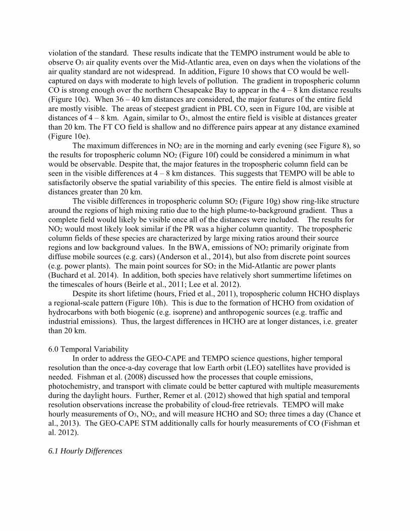
violation of the standard. These results indicate that the TEMPO instrument would be able to observe O3 air quality events over the Mid-Atlantic area, even on days when the violations of the air quality standard are not widespread. In addition, Figure 10 shows that CO would be well-captured on days with moderate to high levels of pollution. The gradient in tropospheric column CO is strong enough over the northern Chesapeake Bay to appear in the 4 – 8 km distance results (Figure 10c). When 36 – 40 km distances are considered, the major features of the entire field are mostly visible. The areas of steepest gradient in PBL CO, seen in Figure 10d, are visible at distances of 4 – 8 km. Again, similar to O3, almost the entire field is visible at distances greater than 20 km. The FT CO field is shallow and no difference pairs appear at any distance examined (Figure 10e).

The maximum differences in NO2 are in the morning and early evening (see Figure 8), so the results for tropospheric column NO2 (Figure 10f) could be considered a minimum in what would be observable. Despite that, the major features in the tropospheric column field can be seen in the visible differences at 4 – 8 km distances. This suggests that TEMPO will be able to satisfactorily observe the spatial variability of this species. The entire field is almost visible at distances greater than 20 km.

The visible differences in tropospheric column SO2 (Figure 10g) show ring-like structure around the regions of high mixing ratio due to the high plume-to-background gradient. Thus a complete field would likely be visible once all of the distances were included. The results for NO2 would most likely look similar if the PR was a higher column quantity. The tropospheric column fields of these species are characterized by large mixing ratios around their source regions and low background values. In the BWA, emissions of NO2 primarily originate from diffuse mobile sources (e.g. cars) (Anderson et al., 2014), but also from discrete point sources (e.g. power plants). The main point sources for SO2 in the Mid-Atlantic are power plants (Buchard et al. 2014). In addition, both species have relatively short summertime lifetimes on the timescales of hours (Beirle et al., 2011; Lee et al. 2012).

Despite its short lifetime (hours, Fried et al., 2011), tropospheric column HCHO displays a regional-scale pattern (Figure 10h). This is due to the formation of HCHO from oxidation of hydrocarbons with both biogenic (e.g. isoprene) and anthropogenic sources (e.g. traffic and industrial emissions). Thus, the largest differences in HCHO are at longer distances, i.e. greater than 20 km. 6.0 Temporal Variability

In order to address the GEO-CAPE and TEMPO science questions, higher temporal resolution than the once-a-day coverage that low Earth orbit (LEO) satellites have provided is needed. Fishman et al. (2008) discussed how the processes that couple emissions, photochemistry, and transport with climate could be better captured with multiple measurements during the daylight hours. Further, Remer et al. (2012) showed that high spatial and temporal resolution observations increase the probability of cloud-free retrievals. TEMPO will make hourly measurements of O3, NO2, and will measure HCHO and SO2 three times a day (Chance et al., 2013). The GEO-CAPE STM additionally calls for hourly measurements of CO (Fishman et al. 2012). 6.1 Hourly Differences

Temporal structure functions yield average trace gas differences as a function of time. The equation is defined as follows:

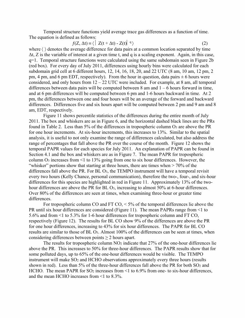
(Z, Δt) Z(t + Δt) - Z(t)q (2) where denotes the average difference for data pairs at a common location separated by time Δt, Z is the variable of interest at a given time t, and q is a scaling exponent. Again, in this case, q=1. Temporal structure functions were calculated using the same subdomain seen in Figure 2b (red box). For every day of July 2011, differences using hourly bins were calculated for each subdomain grid cell at 6 different hours, 12, 14, 16, 18, 20, and 22 UTC (8 am, 10 am, 12 pm, 2 pm, 4 pm, and 6 pm EDT, respectively). From the hour in question, data pairs ± 6 hours were considered, and only hours from 12 – 22 UTC were included. For example, at 8 am, all temporal differences between data pairs will be computed between 8 am and 1 – 6 hours forward in time, and at 6 pm differences will be computed between 6 pm and 1-6 hours backward in time. At 2 pm, the differences between one and four hours will be an average of the forward and backward differences. Differences five and six hours apart will be computed between 2 pm and 9 am and 8 am, EDT, respectively. Figure 11 shows percentile statistics of the differences during the entire month of July 2011. The box and whiskers are as in Figure 6, and the horizontal dashed black lines are the PRs found in Table 2. Less than 5% of the differences in tropospheric column O3 are above the PR for one hour increments. At six-hour increments, this increases to 13%. Similar to the spatial analysis, it is useful to not only examine the range of differences calculated, but also address the range of percentages that fall above the PR over the course of the month. Figure 12 shows the temporal PAPR values for each species for July 2011. An explanation of PAPR can be found in Section 4.1 and the box and whiskers are as in Figure 7. The mean PAPR for tropospheric column O3 increases from <1 to 13% going from one to six hour differences. However, the “whisker” portions show that starting at three hours, there are times when > 70% of the differences fall above the PR. For BL O3, the TEMPO instrument will have a temporal revisit every two hours (Kelly Chance, personal communication), therefore the two-, four-, and six-hour differences for this species are highlighted in red in Figure 11. Approximately 13% of the two-hour differences are above the PR for BL O3, increasing to almost 50% at 6-hour differences. Over 80% of the differences are seen at times, when examining three-hour or greater time differences. For tropospheric column CO and FT CO, < 5% of the temporal differences lie above the PR until six hour differences are considered (Figure 11). The mean PAPRs range from <1 to 5.6% and from <1 to 5.3% for 1-6 hour differences for tropospheric column and FT CO, respectively (Figure 12). The results for BL CO show 9% of the differences are above the PR for one hour differences, increasing to 43% for six hour differences. The PAPR for BL CO results are similar to those of BL O3. Almost 100% of the differences can be seen at times, when considering differences between points ≥ 2 hours apart. The results for tropospheric column NO2 indicate that 27% of the one-hour differences lie above the PR. This increases to 50% for three-hour differences. The PAPR results show that for some polluted days, up to 65% of the one-hour differences would be visible. The TEMPO instrument will make SO2 and HCHO observations approximately every three hours (results shown in red). Less than 5% of the three-hour differences fall above the PR for both SO2 and HCHO. The mean PAPR for SO2 increases from <1 to 6.9% from one- to six-hour differences, and the mean HCHO increases from <1 to 8.3%.

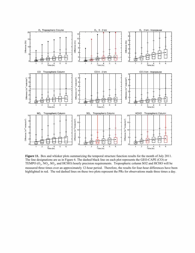
Figure 11. Box and whisker plots summarizing the temporal structure function results for the month of July 2011. The line designations are as in Figure 6. The dashed black line on each plot represents the GEO-CAPE (CO) or TEMPO (O3, NO2, SO2, and HCHO) hourly precision requirements. Tropospheric column SO2 and HCHO will be

measured three times over an approximately 12-hour period. Therefore, the results for four-hour differences have been highlighted in red. The red dashed lines on these two plots represent the PRs for observations made three times a day.

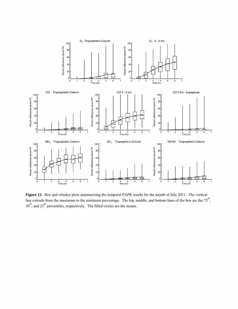
Figure 12. Box and whisker plots summarizing the temporal PAPR results for the month of July 2011. The vertical

line extends from the maximum to the minimum percentage. The top, middle, and bottom lines of the box are the 75th,

50th

, and 25th

percentiles, respectively. The filled circles are the means.

6.2 Temporal context and coverage Similar to the spatial variability analysis, we assess the temporal differences in the

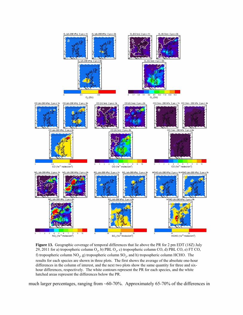
context of a moderate air quality episode (Figure 13). As described in Section 5.3, July 29 was a code orange day where three out of the six DISCOVER-AQ spiral sites violated the EPA O3 standard. Each figure has three plots; the first shows the absolute difference between the column fields at 2 pm EDT (18 UTC) ± one hour. The next plot shows the same quantity ± three hours and the last shows ± six hours. On each plot, the PR requirement is shown as a white contour, and as in Figure 10, the color scales are incremented by the PR of each species. The temporal differences greater than that contour will hypothetically be visible to the instrument.

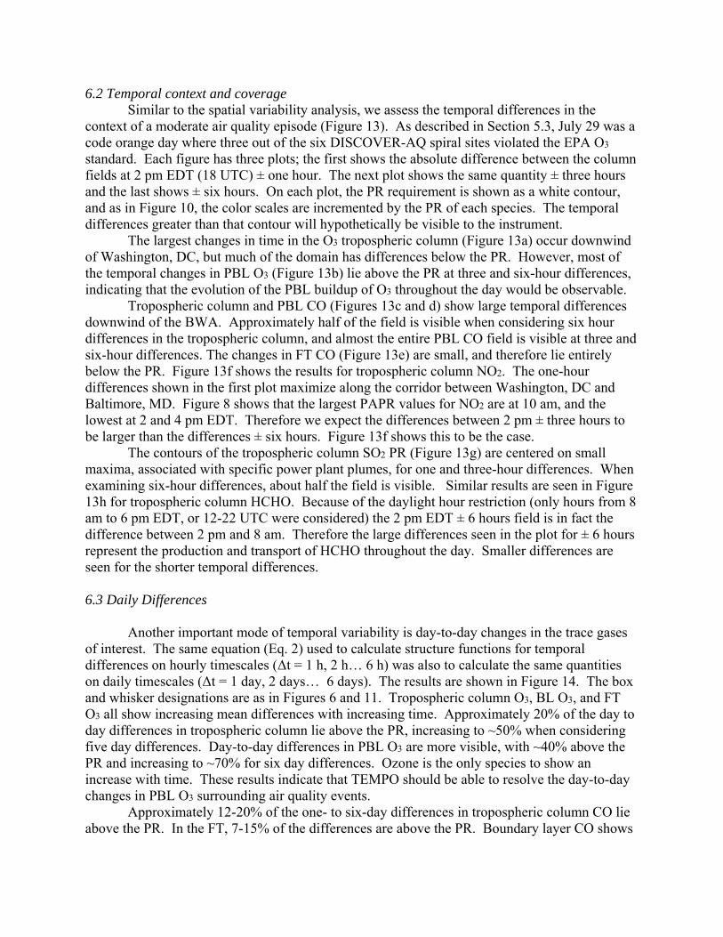
The largest changes in time in the O3 tropospheric column (Figure 13a) occur downwind of Washington, DC, but much of the domain has differences below the PR. However, most of the temporal changes in PBL O3 (Figure 13b) lie above the PR at three and six-hour differences, indicating that the evolution of the PBL buildup of O3 throughout the day would be observable. Tropospheric column and PBL CO (Figures 13c and d) show large temporal differences downwind of the BWA. Approximately half of the field is visible when considering six hour differences in the tropospheric column, and almost the entire PBL CO field is visible at three and six-hour differences. The changes in FT CO (Figure 13e) are small, and therefore lie entirely below the PR. Figure 13f shows the results for tropospheric column NO2. The one-hour differences shown in the first plot maximize along the corridor between Washington, DC and Baltimore, MD. Figure 8 shows that the largest PAPR values for NO2 are at 10 am, and the lowest at 2 and 4 pm EDT. Therefore we expect the differences between 2 pm ± three hours to be larger than the differences ± six hours. Figure 13f shows this to be the case. The contours of the tropospheric column SO2 PR (Figure 13g) are centered on small maxima, associated with specific power plant plumes, for one and three-hour differences. When examining six-hour differences, about half the field is visible. Similar results are seen in Figure 13h for tropospheric column HCHO. Because of the daylight hour restriction (only hours from 8 am to 6 pm EDT, or 12-22 UTC were considered) the 2 pm EDT ± 6 hours field is in fact the difference between 2 pm and 8 am. Therefore the large differences seen in the plot for ± 6 hours represent the production and transport of HCHO throughout the day. Smaller differences are seen for the shorter temporal differences. 6.3 Daily Differences Another important mode of temporal variability is day-to-day changes in the trace gases of interest. The same equation (Eq. 2) used to calculate structure functions for temporal differences on hourly timescales (Δt = 1 h, 2 h… 6 h) was also to calculate the same quantities on daily timescales (Δt = 1 day, 2 days… 6 days). The results are shown in Figure 14. The box and whisker designations are as in Figures 6 and 11. Tropospheric column O3, BL O3, and FT O3 all show increasing mean differences with increasing time. Approximately 20% of the day to day differences in tropospheric column lie above the PR, increasing to ~50% when considering five day differences. Day-to-day differences in PBL O3 are more visible, with ~40% above the PR and increasing to ~70% for six day differences. Ozone is the only species to show an increase with time. These results indicate that TEMPO should be able to resolve the day-to-day changes in PBL O3 surrounding air quality events. Approximately 12-20% of the one- to six-day differences in tropospheric column CO lie above the PR. In the FT, 7-15% of the differences are above the PR. Boundary layer CO shows

much larger percentages, ranging from ~60-70%. Approximately 65-70% of the differences in

Figure 13. Geographic coverage of temporal differences that lie above the PR for 2 pm EDT (18Z) July 29, 2011 for a) tropospheric column O3, b) PBL O3, c) tropospheric column CO, d) PBL CO, e) FT CO,

f) tropospheric column NO2, g) tropospheric column SO2, and h) tropospheric column HCHO. The

results for each species are shown in three plots. The first shows the average of the absolute one-hour differences in the column of interest, and the next two plots show the same quantity for three and six-hour differences, respectively. The white contours represent the PR for each species, and the white hatched areas represent the differences below the PR.

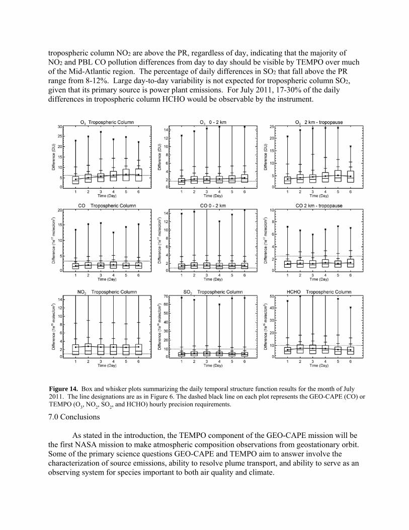
tropospheric column NO2 are above the PR, regardless of day, indicating that the majority of NO2 and PBL CO pollution differences from day to day should be visible by TEMPO over much of the Mid-Atlantic region. The percentage of daily differences in SO2 that fall above the PR range from 8-12%. Large day-to-day variability is not expected for tropospheric column SO2, given that its primary source is power plant emissions. For July 2011, 17-30% of the daily differences in tropospheric column HCHO would be observable by the instrument.

7.0 Conclusions As stated in the introduction, the TEMPO component of the GEO-CAPE mission will be

the first NASA mission to make atmospheric composition observations from geostationary orbit. Some of the primary science questions GEO-CAPE and TEMPO aim to answer involve the characterization of source emissions, ability to resolve plume transport, and ability to serve as an observing system for species important to both air quality and climate.

Figure 14. Box and whisker plots summarizing the daily temporal structure function results for the month of July 2011. The line designations are as in Figure 6. The dashed black line on each plot represents the GEO-CAPE (CO) or TEMPO (O3, NO2, SO2, and HCHO) hourly precision requirements.

In order to estimate the magnitude of variability these missions would observe, we have conducted a structure function analysis of 4-km output from WRF/Chem to quantify simulated variability in the vertical columns of several important trace gases over the course of the month of July, 2011. Structure functions are a useful way to quantify variability, displaying average differences as a function of space or time. When combined with the prospective PRs for GEO-CAPE and TEMPO, the fraction of observable grid points can be determined, as well as the spatial coverage of the observable differences. The model compared well with in-situ observations made during the first deployment of the DISCOVER-AQ field campaign. WRF/Chem slightly overestimates the variability in CO and NO2, and underestimates the variability in HCHO.

The spatial and temporal results for PBL and tropospheric column O3 indicate that the TEMPO instrument would be able to observe O3 air quality events over the Mid-Atlantic area, even on days when the violations of the air quality standard are not widespread. Results for tropospheric column and PBL CO showed that they would be well-captured on days with moderate to high levels of pollution. Differences tended to maximize in the early to mid-afternoon for both species due to the photochemical production of O3 throughout the day as well as the combination of direct emissions and oxidation of VOCs to produce CO. Variability in FT CO was typically low and below the PR. However, there were several occurrences of plumes aloft, entering the BWA. These plumes were characterized by high O3 and CO and were largely visible with respect to the instrument PR (not shown).

Maximum spatial differences in tropospheric column NO2 are in the morning and early evening, corresponding with the local traffic patterns involving morning and evening rush hours. In the BWA, emissions of NO2 primarily originate from diffuse mobile sources, but also from discrete point sources. The main point sources for SO2 in the BWA are power plant plumes, therefore no strong diurnal cycle was observed in the spatial gradients. For NO2, the spatial and temporal results indicate that TEMPO would be able to observe not only the large urban plumes at times of peak production, but also the weaker gradients between rush hours. The spatial and temporal PR for tropospheric column SO2 are lower, therefore only the largest differences, i.e. those associated with power plant plumes, will lie above the PR. Despite its short lifetime, tropospheric column HCHO generally displays a regional-scale spatial pattern. Sources of HCHO include oxidation of hydrocarbons with both biogenic (e.g. isoprene) and anthropogenic sources (e.g. traffic and industrial emissions). Thus, more variability in HCHO is seen at longer distances, i.e. greater than 20 km. Overall, the results indicate that the PRs developed for the GEO-CAPE and TEMPO STMs are sufficient for answering the air-quality relevant science questions they are tasked to address. Acknowledgements This work was supported under the NASA Earth Venture-1 DISCOVER-AQ project and the GEO-CAPE Atmospheric Science Working Group. Contributions from Chinmay Satam for the processing of emissions data are gratefully acknowledged. We also thank Dr. Jack Fishman for his valuable input. References

Anderson, D. C., C. P. Loughner, G. Diskin, A. Weinheimer, T. P. Canty, R. J. Salawitch, H. M. Worden, A. Fried, T. Mikoviny, A. Wisthaler, R.R. Dickerson (2014), Measured and modeled CO and NOy in DISCOVER-AQ: An evaluation of emissions and chemistry over the Eastern US, submitted to Atmospheric Environment. Beirle, S., K. F. Boersma, U. Platt, M. G. Lawrence, and T. Wagner (2011), Megacity Emissions and Lifetimes of Nitrogen Oxides Probed from Space, Science,: 333 (6050), 1737-1739, DOI:10.1126/science.1207824 Bovensmann H., S. Noël , P. Monks, A.P.H. Goede, and J.P. Burrows (2002), The Geostationary Scanning Imaging Absorption Spectrometer (GEOSCIA) Mission: Requirements and Capabilities, Advances In Space Research, Vol. 29, 11, 1849-1859. Bovensmann H. et al. (2004), The Geostationary scanning imaging absorption spectrometer (GeoSCIA) as part of the Geostationary pollution explorer (GeoTROPE) mission: requirements concepts and capabilities, Advances In Space Research, Vol. 34, 4, 694-699. Buchard, V., A. M. Da Silva, P. Colarco, N. Krotkov, R. R. Dickerson, J. W. Stehr, G. Mount, E. Spinei, H. L. Arkinson, and H. He, 2014, Evaluation of GEOS-5 sulfur dioxide simulations during the Frostburg, MD 2010 field campaign. Atmos. Chem. Phys., 14, 1929-1941, doi:10.5194/acp-14-1929-2014. Burrows J.P. et al. (2004), The geostationary tropospheric pollution explorer (GeoTROPE) missions: objects, requirements and mission concept, Advances In Space Research, Vol. 34, 4, 682-687. Chance, K., X. Liu, R. Suleiman, D. Flittner, J. Al-Saadi, S. Janz (2013), Tropospheric Emissions: Monitoring of Pollution (TEMPO), Proc. SPIE 8866, Earth Observing Systems XVIII, 88660D, doi:10.1117/12.2024479. DISCOVER-AQ dataset: doi:10.5067/Aircraft/DISCOVER-AQ/Aerosol-TraceGas Diskin, G. S., J. R. Podolske, G. W. Sachse, and T. A. Slate, 2002:Open-path airborne tunable diode laser hygrometer. Diode Lasers and Applications in Atmospheric Sensing, A. Fried, Ed., International Society for Optical Engineering (SPIE Proceedings, Vol. 4817), 196 – 204, doi:10.1117/12.453736. Emmons, L. K., Walters, S., Hess, P. G., Lamarque, J.-F., Pfister, G. G., Fillmore, D., Granier, C., Guenther, A., Kinnison, D., Laepple, T., Orlando, J., Tie, X., Tyndall, G., Wiedinmyer, C., Baughcum, S. L., and Kloster, S., 2010. Description and evaluation of the Model for Ozone and Related chemical Tracers, version 4 (MOZART-4). Geoscientific Model Development, 3, 43-67. Farmer, D.K., Wooldridge, P.J., Cohen, R.C. 2006. Application of thermal-dissocaition laser induced fluorescence (TD-LIF) to measurement of HNO3, alkyl nitrates, peroxy nitrates, and NO2 fluxes using eddy covariance. Atmospheric Chemistry and Physics 6, 3471-3486.

Fiore, A. M., D. J. Jacob, I. Bey, R. M. Yantosca, B. D. Field, and A. D. Fusco, 2002. Background ozone over the United States in summer: Origin, trend, and contribution to pollution episodes. J. Geophys. Res., 107, D15, 4275, 10.1029/2001JD000982. Fishman, J., K.W. Bowman, J.P. Burrows, A. Richter, K.V. Chance, D.P. Edwards, R.V. Martin, G.A. Morris, R.B. Pierce, J.R. Ziemke, J.A. Al-Saadi, J.K. Creilson, T.K. Schaack, and A.M. Thompson, 2008. Remote sensing of tropospheric pollution from space, Bull. Am. Met. Soc., 89, 805-821. Fishman, J., M. L. Silverman, J. H. Crawford, and J. K. Creilson, 2011. A study of regional-scale variability of in situ and model-generated tropospheric trace gases: Insights into observational requirements for a satellite in geostationary orbit. Atmos. Environ., 45, 4682-4694. Fishman, J., Al-Saadi, J., P. Bontempi, K. Chance, F. Chavez, M. Chin, P. Coble, C. Davis, P. DiGiacomo, A. Eldering, D. Edwards, J. Goes, J. Herman, C. Hu, L. Iraci, D. Jacob, C.C Jordan, S. Kawa, R. Key, X. Liu, S. Lohrenz, A. Mannino, V. Natraj, D. Neil, J. Neu, M. Newchurch, K. Pickering, J. Salisbury, H. Sosik, M. Tzortziou, J. Wang, M. Wang, the GEO-CAPE Atmospheric Science Working Group, and the GEO-CAPE Ocean Science Working Group, 2012. The United States’ Next Generation of Atmospheric Composition and Coastal Ecosystem Measurements: NASA’s Geostationary Coastal and Air Pollution Events (GEO-CAPE) Mission, Bull. Amer. Met. Soc., 93, 1547-1566. Grell, G. A., Peckham, S. E., Schmitz, R., McKeen, S. A., Frost, G., Skamarock, W. C., Eder, B., 2005. Fully coupled online chemistry within the WRF model. Atmospheric Environment 39, 6957-6975. Guenther, A. B., Jiang, X., Heald, C. L., Sakulyanontvittaya, T., Duhl, T., Emmons, L. K., and Wang, X. (2012), The Model of Emissions of Gases and Aerosols from Nature version 2.1 (MEGAN2.1): an extended and updated framework for modeling biogenic emissions, Geosci. Model Dev., 5, 1471-1492, doi:10.5194/gmd-5-1471-2012. Harris, D., Foufoula-Georgiou, E., Droegemeier, K. K., Levit, J. J., 2001. Multiscale statistical properties of a high resolution precipitation forecast. Journal of Hydrometeorology 2, 406-418. Houyoux, M., R., and Vukovich, J. M., 1999. Updates to the Sparse Matrix Operator Kernel Emissions (SMOKE) modeling system and integration with models-3. Presented at The Emission Inventory: Regional Strategies for the Future, Air and Waste Management Association, Raleigh, NC. Kim, J. (2012), GEMS (Geostationary Environment Monitoring Spectrometer) onboard the GeoKOMPSAT to Monitor Air Quality in high Temporal and Spatial Resolution over Asia-Pacific Region", EGU General Assembly Conference Abstracts. Vienna, Austria, (2012). Kim, S.-W., A. Heckel, S. A. McKeen, G. J. Frost, E.-Y. Hsie, M. K. Trainer, A. Richter, J. P. Burrows, S. E. Peckham, and G. A. Grell (2006), Satellite-observed U.S. power plant NOx

emission reductions and their impact on air quality, Geophys. Res. Lett., 33, L22812, doi:10.1029/2006GL027749. Lee, C., R. V. Martin, A. van Donkelaar, H. Lee, R. R. Dickerson, J. C. Hains, N. Krotkov, A. Richter, K. Vinnikov, and J. J. Schwab (2011), SO2 emissions and lifetimes: Estimates from inverse modeling using in situ and global, space‐based (SCIAMACHY and OMI) observations, J. Geophys. Res., 116, D06304, doi:10.1029/2010JD014758 Lindinger, W., Hansel, A., Jordan, A. 1998. Proton-transfer-reaction mass spectrometry (PTR-MS): on-line monitoring of volatile organic compounds at pptv levels. Chemical Society Reviews, 27 (5): 347-354. Loughner, C. P., Lary, D. J., Sparling, L. C., Cohen, R. C., DeCola, P., Stockwell, W. R., 2007. A method to determine the spatial resolution required to observe air quality from space, IEEE Transactions on Geosciences and Remote Sensing 45, 1308-1314. National Research Council (NRC), 2007. Earth Science and Applications from Space: National imperatives for the next decade and beyond, National Academy Press, Washington, D.C., pp. 428. Parrish, D. D., et al. (2009), Overview of the Second Texas Air Quality Study (TexAQS II) and the Gulf of Mexico Atmospheric Composition and Climate Study (GoMACCS), J. Geophys. Res., 114, D00F13, doi:10.1029/2009JD011842. Remer, L., S. Mattoo, R.C. Levy, A. Heidinger, R.B. Pierce, and M. Chin, 2012. Retrieving aerosol in a cloudy environment: Aerosol availability as a function of spatial and temporal resolution, Atmos. Meas. Tech. Discuss., 5, 627-662. Ridley, B.A., Grahek, F.E. 1990. A small, low flow, high-sensitivity reaction vessel for NO chemiluminescence detectors. Journal of Atmospheric and Ocean Technology, 7, 307-311. Sachse, G.W., Hill, G.F., Wade, L.O., Perry, M.G. 1987. Fast-response, high-precision carbon monoxide sensor using a tunable diode laser absorption technique. Journal of Geophysical Research 92, 2071–2081. Sachse, G.W., Harriss, R.C., Fishman, J., Hill, G.F., Cahoon, D.R. 1998. Carbon monoxide over the Amazon basin during the 1985 dry season. Journal of Geophysical Research 93, 1422– 1430. Skamarock, W. C., J. B. Klemp, J. Dudhia, D. O. Gill, D. M. Barker, W. Wang, and J. G. Powers, 2005: A description of the Advanced Research WRF Version 2. NCAR Tech Notes-468+STR. Trainer, M., D. D. Parrish, P. D. Goldan, J. Roberts, F.C. Fehsenfeld, 2000: Review of observation-based analysis of the regional factors influencing ozone concentrations. Atmos. Environ., 34, 2045-2061.

U.S. Environmental Protection Agency, 2009. Air quality index: a guide to air quality and your health. Environmental Protection Agency, Research Triangle Park, NC. Office of Air Quality Planning and Standards. U.S. Environmental Protection Agency, Office of Air Quality Planning and Standards, Outreach and Information Division, Report EPA-456/R-09-002, 11 pp. U.S. Environmental Protection Agency, 2011. Regulatory Impact Analysis. In: Final National Ambient Air Quality Standard for Ozone. http://www.epa.gov/air/ozonepollution/pdfs/201107_OMBdraft-OzoneRIA.pdf. U.S. Environmental Protection Agency, 2012: User Guide for MOVES2010b. Office of Transportation and Air Quality, US Environmental Protection Agency, Washington DC, EPA-420-B-12-001b, 202 pp. Vay, et al., 2011. Patterns of CO2 and radiocarbon across high northern latitudes during IPY 2008, J. Geophys. Res. 116,doi:10.1029/2011JD015643. Weibring, P., D. Richter, A. Fried, J.G. Walega, and C. Dyroff, Ultra-High-Precision Mid-IR Spectrometer II: System Description and Spectroscopic Performance, Appl. Phys. B, doi:10.1007/s00340-006-2300-4, 2006. Weibring, P., D. Richter, J.G. Walega, and A. Fried, First Demonstration of a High Performance Difference Frequency Spectrometer on Airborne Platforms, Optics Express, 15(21),13,476 13,495, 2007. Wiedinmyer, C., S. K. Akagi, R. J. Yokelson, L. K. Emmons, J. A. Al-Saadi, J. J. Orlando, and A. J. Soja, 2011: The Fire INventory from NCAR (FINN): a high resolution global model to estimate the emissions from open burning. Geosci. Model Dev., 4, 625-641, doi:10.5194/gmd-4-625-2011. Yegorova, E. A., D. J. Allen, C. P. Loughner, K. E. Pickering, and R. R. Dickerson (2011), Characterization of an eastern U.S. severe air pollution episode using WRF/Chem, J. Geophys. Res., 116, D17306, doi:10.1029/2010JD015054.