Spatial and isotopic niche partitioning during winter … · Spatial and isotopic niche partitioning during ... Spatial and isotopic niche partitioning during winter in chinstrap

Spatial and isotopic niche partitioning during winter in chinstrapand Adelie penguins from the South Shetland Islands

JEFFERSON T. HINKE,1,� MICHAEL J. POLITO,2,3 MICHAEL E. GOEBEL,1 SHARON JARVIS,4 CHRISTIAN S. REISS,1

SIMON R. THORROLD,3 WAYNE Z. TRIVELPIECE,1 AND GEORGE M. WATTERS1

1Antarctic Ecosystem Research Division, Southwest Fisheries Science Center, National Marine Fisheries Service,National Oceanic and Atmospheric Administration, La Jolla, California 92037 USA

2Department of Oceanography and Coastal Sciences, Louisiana State University, Baton Rouge, Louisiana 70803 USA3Biology Department, Woods Hole Oceanographic Institution, Woods Hole, Massachusetts 02543 USA

4Aviculture Department, SeaWorld, Orlando, Florida 32821 USA

Citation: Hinke, J. T., M. J. Polito, M. E. Goebel, S. Jarvis, C. S. Reiss, S. R. Thorrold, W. Z. Trivelpiece, and G. M. Watters.

2015. Spatial and isotopic niche partitioning during winter in chinstrap and Adelie penguins from the South Shetland

Islands. Ecosphere 6(7):125. http://dx.doi.org/10.1890/ES14-00287.1

Abstract. Closely related species with similar ecological requirements should exhibit segregation along

spatial, temporal, or trophic niche axes to limit the degree of competitive overlap. For migratory marine

organisms like seabirds, assessing such overlap during the non-breeding period is difficult because of long-

distance dispersal to potentially diffuse foraging habitats. Miniaturization of geolocation devices and

advances in stable isotope analysis (SIA), however, provide a robust toolset to quantitatively track the

movements and foraging niches of wide ranging marine animals throughout much of their annual cycle.

We used light-based geolocation tags and analyzed stable carbon and nitrogen isotopes from tail feathers

to simultaneously characterize winter movements, habitat utilization, and overlap of spatial and isotopic

niches of migratory chinstrap (Pygoscelis antarctica) and Adelie (P. adeliae) penguins during the austral

winter of 2012. Chinstrap penguins exhibited a higher diversity of movements and occupied portions of the

Southern Ocean from 1388 W to 308 W within a narrow latitudinal band centered on 608 S. In contrast, all

tracked Adelie penguins exhibited smaller-scale movements into the Weddell Sea and then generally along

a counter-clockwise path as winter advanced. Inter-specific overlap during the non-breeding season was

low except during the months immediately adjacent to the summer breeding season. Intra-specific overlap

by chinstraps from adjacent breeding colonies was higher throughout the winter. Spatial segregation

appears to be the primary mechanism to maintain inter- and intra-specific niche separation during the non-

breeding season for chinstrap and Adelie penguins. Despite low spatial overlap, however, the data do

suggest that a narrow pelagic corridor in the southern Scotia Sea hosted both chinstrap and Adelie

penguins for most months of the year. Shared occupancy and similar isotopic signatures of the penguins in

that region suggests that the potential for inter-specific competition persists during the winter months.

Finally, we note that SIA was able to discriminate eastward versus westward migrations in penguins,

suggesting that SIA of tail feathers may provide useful information on population-level distribution

patterns for future studies.

Key words: Antarctica; geolocation; migration; niche; Pygoscelis adeliae; Pygoscelis antarctica; stable isotope; winter.

Received 8 September 2014; revised 2 March 2015; accepted 3 April 2015; final version received 6 May 2015; published

29 July 2015. Corresponding Editor: B. Maslo.

Copyright: � 2015 Hinke et al. This is an open-access article distributed under the terms of the Creative Commons

Attribution License, which permits unrestricted use, distribution, and reproduction in any medium, provided the

original author and source are credited. http://creativecommons.org/licenses/by/3.0/

� E-mail: [email protected]

v www.esajournals.org 1 July 2015 v Volume 6(7) v Article 125

INTRODUCTION

Ecological theory predicts that closely relatedspecies with similar ecological requirementsshould exhibit niche partitioning to limit thedegree of competitive overlap where they co-occur (Ricklefs and Miller 1999). For example,because many sympatric colonial seabird assem-blages have restricted foraging ranges during thebreeding season they are often used as modelassemblages to study mechanisms of inter-specific and intra-specific niche partitioning inenvironments with limited resources (Lewis et al.2001, Wilson 2010). These studies have shownthat competitive overlap may be reduced amongsympatric competitors via segregation along thetrophic axes of species’ respective foraging niches(e.g., relying on different food resources; Croxallet al. 1997, Cherel et al. 2008). In addition,segregation in spatial (e.g., vertical or horizontaldisplacement) and temporal (e.g., shifts in peakresource or habitat use) niche axes can alsoeffectively reduce competition between breedingseabirds (Wilson 2010, Connan et al. 2014).Foraging niche segregation is also evident be-tween neighboring populations of the samespecies as the potential for intra-specific compe-tition is often higher than competition amongcongenerics (Masello et al. 2010).

Most studies on the foraging niches of seabirdshave focused on the breeding season because ofease of access to study animals and the expecta-tion that competition during the breeding seasonis exacerbated by the increased demands ofraising offspring and the constraints of centralplace foraging. Studies examining foraging ecol-ogy during the non-breeding periods are lesscommon, despite recognition that foraginggrounds during the non-breeding period maycontain high densities of competitors (e.g.,Karnovsky et al. 2007). The miniaturization ofanimal-borne loggers has significantly improvedthe ability to track the long-distance movementsof seabirds during the non-breeding season (e.g.,Kooyman et al. 2000, Clarke et al. 2003, Bost et al.2004, Shaffer et al. 2006, Quillfeldt et al. 2012). Inaddition, advances in the use of stable isotopeanalysis (SIA), which is based on the principlethat animals ‘‘are what and where they eat’’(Inger and Bearhop 2008, Bond and Jones 2009),now provide the ability to estimate foraging

niches from tissues grown during the non-breeding period when individuals are away fromland (e.g., Polito et al. 2011a). In combination,direct tracking and SIA provide a robust toolsetto quantitatively track the movements andforaging niches of wide-ranging marine organ-isms, including seabirds, throughout much oftheir annual cycle (Gonzalez-Solıs et al. 2007,Block et al. 2011, Polito et al. 2011a, Seminoff etal. 2012). Interestingly, recent studies using theapproaches above have noted clear patterns ofspatial and temporal foraging niche segregationwithin and between sympatric seabird speciesduring the winter months when they are awayfrom breeding colonies (Thiebot et al. 2011,Ratcliffe et al. 2014). These results suggest thatsome seabird assemblages have evolved behav-ioral mechanisms that help to limit inter andintra-specific competitive overlap during thenon-breeding period.

In this study we focus on the movements ofchinstrap (Pygoscelis antarctica) and Adelie (P.adeliae) penguins during the non-breeding season(March–October; hereafter ‘‘winter’’ unless oth-erwise specified). Both species exhibit populationdeclines in the Antarctic Peninsula region inresponse to climate warming, consequent loss ofsea ice, and reductions in the availability ofAntarctic krill (Euphausia superba; Trivelpiece etal. 2011, Lynch et al. 2012). Habitat availabilityand foraging conditions encountered duringwinter may be important drivers of the observedchanges in penguin abundance in the AntarcticPeninsula region (Hinke et al. 2007), furthersuggesting the need to examine dispersal routesand foraging habitats of these species duringwinter. A constraint of such monitoring, howev-er, is that Adelie and chinstrap penguins exhibitseasonal migrations between summer breedingsites and winter foraging habitats that may beseparated by hundreds or thousands of kilome-ters (Wilson et al. 1998, Clarke et al. 2003,Trivelpiece et al. 2007, Ballard et al. 2010, Biuwet al. 2010). Accordingly, direct comparisons ofmarine habitat use and foraging niches of thesesympatric competitors during the non-breedingseason remain an important gap in our under-standing of Adelie and chinstrap penguin ecol-ogy.

On a broad-scale, ship-based observationssuggest that these two species may segregate


HINKE ET AL.

winter foraging areas based on the presence ofsea ice. Adelie penguins are typically observed inmarginal ice zones while chinstrap penguinsoften are observed in open waters north of theice edge (Ainley et al. 1994). Winter trackingstudies have confirmed seasonal occupancy of icezones for Adelie penguins (Clarke et al. 2003,Ballard et al. 2010, Dunn et al. 2011, Erdmann etal. 2011) while chinstrap penguins tend to be inareas typically free of ice (Wilson et al. 1998,Trivelpiece et al. 2007, Biuw et al. 2010). Even so,the previous tracking studies have examined thewinter movements of each species in isolation.Consequently addressing spatial segregationduring the non-breeding season has been ham-pered by low sample sizes and a lack of temporal(year of study) and spatial (breeding populationexamined) overlap between studies.

Here we report on research to simultaneouslytrack individuals from two breeding colonies ofAdelie and chinstrap penguins in the SouthShetland Islands, Antarctic Peninsula with archi-val geolocation tags and examine foraging nichespace using SIA. Our goals are to assess thedegree and mechanism (spatial, temporal and/or

trophic) of foraging niche partitioning that occursduring the non-breeding periods, both betweenthese two species from the same breeding colonyin Admiralty Bay, King George Island, as well asbetween members of the same species (chinstrappenguins) from Admiralty Bay and Cape Shir-reff, Livingston Island; these colonies are sepa-rated by 120 km (Fig. 1). We predict that spatialsegregation of foraging areas will occur betweenspecies based on previously observations ofdifferences in foraging areas evident during thebreeding period (Wilson 2010) and winterobservations that indicate Adelie penguins aremore commonly observed in marginal ice zoneswhile chinstrap penguins occupy open watersnorth of the ice edge (Ainley et al. 1994). Becauseneighboring populations of con-specifics likelyoccupy the same ecological niche, we predict thatchinstrap penguins from different colonies willexhibit relatively higher overlap in winter forag-ing areas and isotopic niche space, as intra-specific segregation would be expected to occurwithin a shared habitat rather than occupation ofdistinct habitats (Thiebot et al. 2011, Thiebot et al.2012, but see Ratcliffe et al. 2014).

Fig. 1. Study area and location of tagging sites, indicated by black dots, at Cape Shirreff, Livingston Island and

Admiralty Bay, King George Island, South Shetland Islands, Antarctica.


HINKE ET AL.

METHODS

TaggingChinstrap and Adelie penguins from Cape

Shirreff, Livingston Island (62.468 S, 60.798 W)and Admiralty Bay, King George Island (62.218 S,58.428 W; Fig. 1) were captured during the 2011/12 breeding season (Table 1) and fitted withLotek Nano-Lat 2900-series archival geolocationtags (hereafter GLS; Lotek Wireless, St. Johns,Newfoundland, Canada) to monitor dispersaland habitat utilization. Tagging was concentratedin one small sub-colony for each species at eachsite to help minimize search effort and maximizerecovery rates in the following spring. The GLStags were affixed to a white plastic ring bandwith two small plastic cable wraps and the ringband was then fitted to the right tarsus of eachbird. Each GLS tag had dimensions 8 3 15 3 7mm and weighed 2 g in air. The tags provideddaily estimates of latitude, longitude, and surfacetemperature.

Effects of tagsThe attachment of external archival tags to

seabirds is a common practice among fieldresearch programs. Miniaturization of tags andthe ability to use tarsus bands for attachment arecritical for eliminating damage to the plumage byadhesives. Based on observations in the field, wenote that the attachment method, similar to thatof Ballard et al. (2010), and the size of the tagused in this study appeared to have had minorimpacts on our study penguins. The observedreturn rate, roughly 70% (Table 1), was consistentwith expected returns given mortality rates forPygoscelid penguins in the region (Hinke et al.2014). Observers in the field confirmed that nobirds presented serious injury and exhibited onlyminor callusing from over 10 months of wear.

Observers also confirmed normal breeding be-haviors and successful breeding attempts amongmany tracked birds. We note, however, that noeffort was made to identifiably mark or furtherdisturb the birds once the GLS tag was removedand the tail feather collected. We thereforeassume the impacts of tagging were minor andhad no significant bias on the large-scale trackingor stable isotope data collected.

Bias and error in locationTo estimate bias and error in position estimates

from the GLS tags, we used data from four GLScontrol tags that were either fixed-positiondeployments at Cape Shirreff (N ¼ 2) or animal-borne deployments (N ¼ 2) with simultaneousARGOS-based satellite estimates of position thatserved as mobile controls. The estimation proce-dure for the bias correction and location error inthe GLS data is provided in Appendix A.Preliminary analysis of the control-tag dataindicated bias in location was present, particu-larly for latitude estimates during mid-wintermonths. We therefore used the control-tag data toestimate weekly bias corrections for correctingraw data from tracked animals, and we estimat-ed weekly errors in the control-tag data for inputinto modeling penguin movement tracks (seeMaterials and methods: Habitat utilization). All datafrom the tagged penguins were bias-correctedand then filtered with a speed filter (Freitas et al.2008), assuming maximum sustained swimspeeds of 2 m�s�1, to remove anomalous datapoints prior to further analyses.

Habitat utilizationHabitat utilization, defined here as the pro-

portion of time spent in a specified grid cell foreach month, was estimated via a four-stepprocess. First, we fitted a state-space model

Table 1. Summary information on number of deployments, recoveries, and data collection from GLS tags,

including mean and range of deployment durations.

Tagging locale Species

No. tags No. tags used for analysis Duration of deployments (d)

Deployed Recovered Downloaded Winter habitat Isotope period� Mean Range

Admiralty Bay Adelie 51 36 34 29 19 211 32–423Admiralty Bay Chinstrap 50 30 20 19 16 141 23–290Cape Shirreff Chinstrap 61 46 37 34 21 121 30–313

� Tag failures prior to the isotope study period, assumed to be 40-100 days after molt initiation, reduced the sample sizes oftags during of the isotope period relative to those used for habitat mapping.


HINKE ET AL.

(Johnson et al. 2008) to the bias-corrected datafrom each tag to produce hourly estimates ofprobable location. The model was fitted using theR (R Core Team 2012) package ‘crawl’ (Johnsonet al. 2008). As an error structure for the model,we used the weekly estimates of location error asdescribed in detail in the Appendix A. Second,based on the parameters of the fitted model, wegenerated 100 alternative track lines, with posi-tion estimates for each hour, for all tags. The setof alternative track lines was generated toaccount for the uncertainty in individual locationestimates, and we assumed that the set of 100provided a sufficient sample to characterizeuncertainty in habitat use. Third, we aggregatedthe 100 probable track lines from all individualsand split the dataset into monthly components.The monthly temporal resolution reported here isarbitrary, but we felt that this scale best integrat-ed across the movement rates and position errorswhile providing sufficient temporal resolution toidentify movement patterns on a large scale (e.g.,Thiebot et al. 2011). Finally, we overlaid theaggregated monthly data onto a grid to estimatethe proportion of time spent in any grid cell. Forthis analysis, we used a grid-cell size of 38

longitude by 28 latitude based on the maximumlocation error in the control-tag data (AppendixA). We note that the relatively large size of thisgrid cell precludes fine-scale differentiation ofhabitat use; for example, sea ice could provide anatural boundary separating Adelie and chin-strap penguins in a particular grid cell. However,we assume that shared occupancy of a particulargrid cell is indicative of the importance of thatgeneral area to all individuals and will hereafterrefer to that shared occupancy of the grid cell asoverlap in habitat use. With this caveat andbroad-scale frame of reference, we do not focuson individual migratory routes or movementrates but prefer a more probabilistic approach toidentify frequently occupied areas based onlikely positions given the uncertain raw estimatesof position. We also limit our discussion of basin-scale movements to an arbitrary monthly timeframe to align the large spatial scale with arelatively long-term temporal scale of resolution.

We used the simple overlap index of Schoener(1970) to quantify the degree of inter-specific(chinstrap versus Adelie penguin) and intra-specific (chinstrap penguins from Cape Shirreff

and Admiralty Bay) habitat overlap, where avalue of one indicates identical occupancy of gridcells for the two groups being compared, while avalue of zero indicates the absence of overlap. Wecalculated the overlap index for each monthusing two different metrics of habitat utilization.First, we calculated a ‘‘spatial’’ overlap indexbased on the proportion of time spent in eachgrid cell. This calculation measured the extent ofshared occupancy of grid cells during the timeperiod of interest. The second index measuredoverlap on an ‘‘individual’’ basis by calculatingthe proportion of individuals from the taggedsample of each species that occupied each gridcell during the time period of interest.

Environmental covariatesSea ice is a critical component of marine

habitat in the Southern Ocean. After the breedingseason Adelie penguins typically molt and foragein concentrated pack ice (50–80%; Ballard et al.2010, Dunn et al. 2011), while chinstrap penguinsare generally observed north of the sea-ice edgein open water (Ainley et al. 1994). Therefore,these species would be expected to track theadvance and retreat of sea ice. We used meanmonthly sea-ice concentration data for 2012,reported on a 0.258 latitude-longitude grid,available from the National Snow and Ice DataCenter (http://nsidc.org/data/polaris/), to esti-mate the extent of sea ice throughout the rangeof marine habitats used by the tagged penguins.We used contours of 15% and 50% sea-iceconcentrations to compare with the spatialdistributions of tagged individuals. The 15%contour represents an effective ice edge and the50% contour was chosen as a northern limit forAdelie penguin. We hypothesized that chinstrappenguins would occupy marine habitats mainlynorth of the 15% sea-ice concentration margin,while Adelie penguins would occupy habitatsmainly south of 50% sea-ice concentration mar-gin. Finally, we used sea-surface temperaturedata (Reynolds et al. 2002 ) for 2012, provided ona 18 latitude-longitude grid by the Earth SystemResearch Laboratory (http://www.esrl.noaa.gov/psd/) and daily estimates of surface temperaturesrecorded by the GLS tags to identify broad-scalethermal ranges used by the tagged penguins. Forplotting, all isotherms and ice contours weresmoothed using a loess smoother.


HINKE ET AL.

Tail-feather samplingA single, central tail feather was plucked from

all birds that were recaptured with a GLS tag toassess penguin foraging ecology during winterusing SIA. Feathers are metabolically inertfollowing synthesis and therefore encapsulatean isotopic record of avian diets and foraginghabitat use from when and where they weregrown (Hobson 1999, Ramos and Gonzalez-Solıs2012). Therefore, we used data on the timing andrate of growth of tail feathers from a captivestudy, detailed in Appendix B, of Adelie pen-guins to select a 0.5-cm section from the shaft ofeach tail feather from GLS tracked individualsthat was grown approximately 59611 and 69620days following the onset of molt for chinstrapand Adelie penguins, respectively. Given uncer-tainty in growth rates of tail feathers in the wild,isotopic turnover rates in feathers (see Discus-sion), and error in estimates of position from thetracking data (Appendix A), we used a moreconservative 95% confidence interval range of40–100 days (Appendix B) following the onset ofmolt to compare the isotopic composition of tailfeathers with the spatial distribution of animals.Thus, the section of tail feather used for SIAreflects a growth period from late March to earlyJune when penguins are migrating to and/orinhabiting their winter foraging areas. We re-stricted our isotopic analyses of tail feathers to 18Adelie (7 male and 11 female) and 34 chinstrap(19 male and 15 female) penguins. These indi-viduals had GLS tracking data that fell within thewindow of tail-feather synthesis and isotopicincorporation (i.e., 40–100 days following theonset of molt).

The feather sections used for SIA were cleanedusing a 2:1 chloroform:methanol rinse, air-dried,and cut into small fragments with stainless steelscissors. We flash-combusted (Costech ECS4010elemental analyzer) approximately 0.5 mg ofeach sample loaded into tin cups and analyzedfor carbon and nitrogen isotopes (d13C and d15N)through interfaced Thermo Scientific Delta VPlus continuous-flow stable isotope ratio massspectrometer (CFIRMS). Raw d values werenormalized on a two-point scale using glutamicacid reference materials with low and highvalues (USGS-40: d13C ¼ �26.4%, d15N ¼�4.5%; USGS-41: d13C ¼ 37.6%, d15N ¼ 47.6%).Sample precision, based on repeated sampling of

reference materials, was 0.1% and 0.2% for d13Cand d15N, respectively. Stable isotope ratios areexpressed in d notation in per mil units (%),according to the following equation:

dX ¼ ½ðRsample=RbaseÞ � 1�3 1000

where X is 13C or 15N and Rsample is thecorresponding ratio 13C/12C or 15N/14N. The Rbase

values were based on the Vienna PeeDeeBelemnite (VPDB) for d13C and atmospheric N2

for d15N.

Isotopic niche and dietary modelingWe followed an isotopic niche approach when

using SIA to test for inter- and intraspecificforaging niche partitioning (Newsome et al.2007). When presented as bi-plots, stable isotopevalues delineate the trophic (d15N) and habitat-use (d13C) axes of an isotopic niche space (Bodeyet al. 2013), which is comparable, although notidentical, to the ecological niche space defined byHutchinson (1959). We used linear models to testfor difference in d13C and d15N values betweenspecies from the same breeding site as well aswithin species between breeding sites (chinstrappenguins only). In addition, we tested fordifferences in species-specific foraging nichesbetween discrete winter foraging areas by clas-sifying chinstrap penguins into two groups (eastand west) based on the mean bearing from thetagging location during the period of feathersynthesis. We compared the size and degree ofoverlap in bivariate isotopic niche space (d13Cand d15N) occupied by chinstrap and Adeliepenguins using two methods. First, we calculatedthe standard ellipse area corrected for samplesize (SEAc; Jackson et al. 2011). The SEAc metricis equivalent to a bivariate standard deviationand can be interpreted as a measure of the coreisotopic niche of a population (Jackson et al.2011). We further calculated a Bayesian approx-imation of SEAc with corresponding 95% credi-bility intervals (SEAb; Jackson et al. 2011) toquantify uncertainty in core isotopic niche areas.Second, we constructed convex hulls to estimatethe smallest total isotopic niche area (TA) thatcontained all individuals in the isotopic space.The TA metric can be interpreted as a measure ofthe total isotopic niche of a population (Laymanet al. 2007). Using the graphical SEAc and TAmetrics we calculated core and total niche-


HINKE ET AL.

overlap indices between groups as both apercentage of overall isotopic area (i.e., nichespace) as well as the proportion of individuals ofone group encompassed by another group’sisotopic area (Hammerschlag-Peyer et al. 2011,Jackson et al. 2011). Isotopic niche modeling wasimplemented in R (R Core Team 2012).

RESULTS

After one winter of deployment, we recovered112 tags (69% of deployments) and successfullyretrieved location data from 34 Adelie penguinsand 57 chinstrap penguins (Table 1). We elimi-nated 5 Adelie penguins and 5 chinstrap pen-guins from our analysis due to premature tagfailure (prior to the molt) or corrupted locationdata. The remaining 29 Adelie penguins, all fromAdmiralty Bay, had a mean active deployment of211 6 123 (SD) days. Chinstrap penguins fromAdmiralty Bay (N ¼ 19) had a mean activedeployment of 141 6 78 (SD) and chinstrapsfrom Cape Shirreff (N ¼ 33) had a mean activedeployment of 121 6 67 (SD) days.

Habitat utilizationDuring winter, chinstrap penguins generally

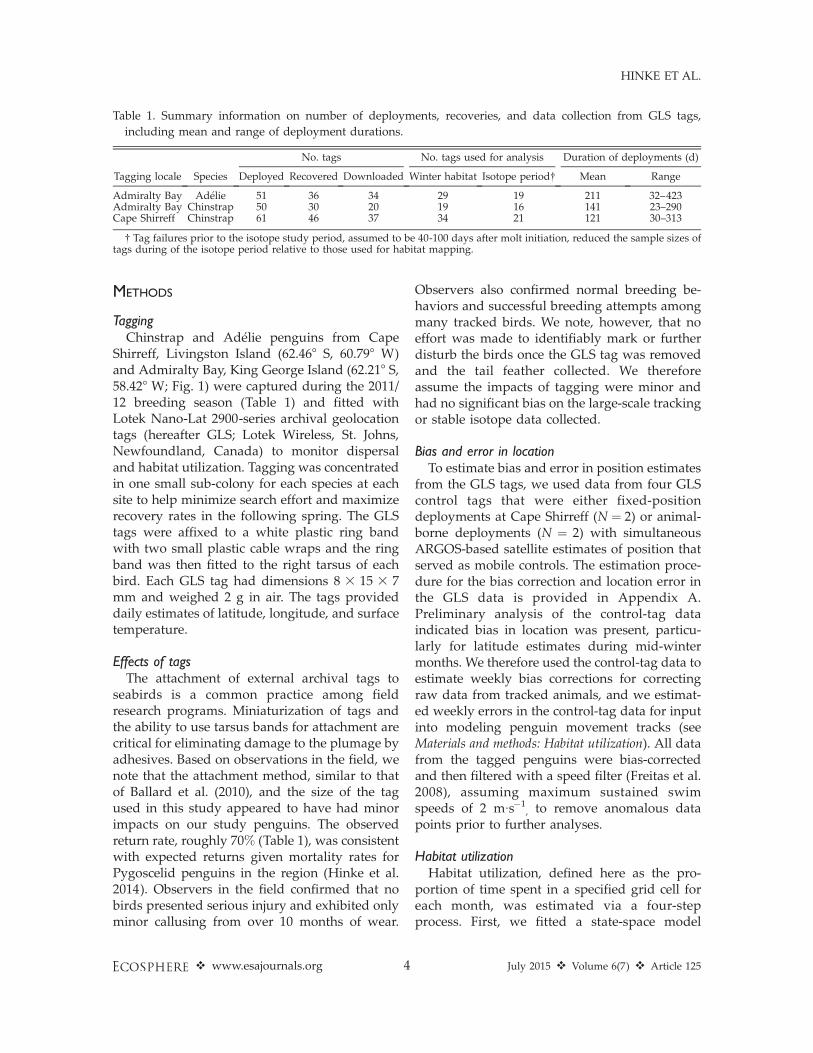
exhibited a higher diversity of individual move-ment patterns, undertook longer-distance move-ments, and occupied a broader geographic rangeof marine habitats than Adelie penguins. Chin-strap penguins exhibited two main movementmodes, migrating either west or east fromtagging locations in the South Shetland Islands(Figs. 2A, 3). The majority of chinstraps fromCape Shirreff (82%) and Admiralty Bay (63%)migrated west into the Pacific sector of theSouthern Ocean while the remainder moved eastinto the south Atlantic sector. Individual chin-strap penguins migrated as far west as 1388 Wand as far east as 308 W prior to instrumentfailure, representing maximum point-to-pointgreat-circle distances from tagging locations of3900 km and 1960 km, respectively. Thesemaximum distances were achieved within 3months of the end of the molting period andprior to late June/early July when the datasuggest that the birds reversed course andinitiated their return migrations (Figs. 2A, 3).The latitudes used by chinstraps throughout thewinter, whether moving east or west from the

South Shetland Islands, remained in a relativelynarrow band between 608 S and 658 S (Fig. 2B),generally bounded on the south by advancingsea ice edge and to the north by the 28C isotherm(Fig. 3). Average daily sea surface temperaturesrecorded by the GLS tags (1.38C 6 2.88C mean 6

SD) and the spatial distribution of those temper-atures (Appendix C) corroborate this broad-scalecharacterization of winter habitat.

In contrast, all Adelie penguins tagged in thisstudy exhibited a counter-clockwise movementpattern (Figs. 2C, D, 3). After the breedingseason, all tagged individuals moved southeastinto the NW Weddell Sea where, presumably, allindividuals molted (e.g., Dunn et al. 2011).Incomplete data for the month of March, due tolocation errors associated with the equinox(Ekstrom 2004), precluded clear interpretationof movements immediately following the molt,but by mid-April most individuals had returnedas far north at 608 S (Fig. 2D). Thereafter,movement was relatively restricted and allindividuals appeared to remain in the southernScotia Sea and northwestern Weddell Sea be-tween 508 W and 608 W longitude, withoutappreciable directional movement until returntrips to the breeding colonies commenced by lateSeptember. The mean great circle distance to thetagging location in Admiralty Bay during themid-winter period (June–August) for all Adeliepenguins combined was 555 6 248 km. Thetracking data suggest that Adelie penguinsoccupied habitats centered on ice concentrationsbetween 15 and 50% for most of the winter (Fig.3). Average daily sea surface temperaturesrecorded by the GLS tags (�1.2 6 4.98C;Appendix C), further suggest the occupation ofhabitats with sea ice cover.

The level of spatial overlap differed betweenand within species. Due to the large-scalelongitudinal movements of most chinstrap pen-guins in ice-free waters, the index of spatialoverlap of winter habitats used by chinstrap andAdelie penguins was relatively low and generallydecreased as winter progressed (Fig. 4A). Ingeneral, the probability of co-occurrence ofAdelie and chinstrap penguins in a given gridcell was low (,0.004) throughout the winter (Fig.5), but areas of co-occurrence were consistentlylocated in the confluence of the Weddell andScotia Seas between Elephant Island and the


HINKE ET AL.

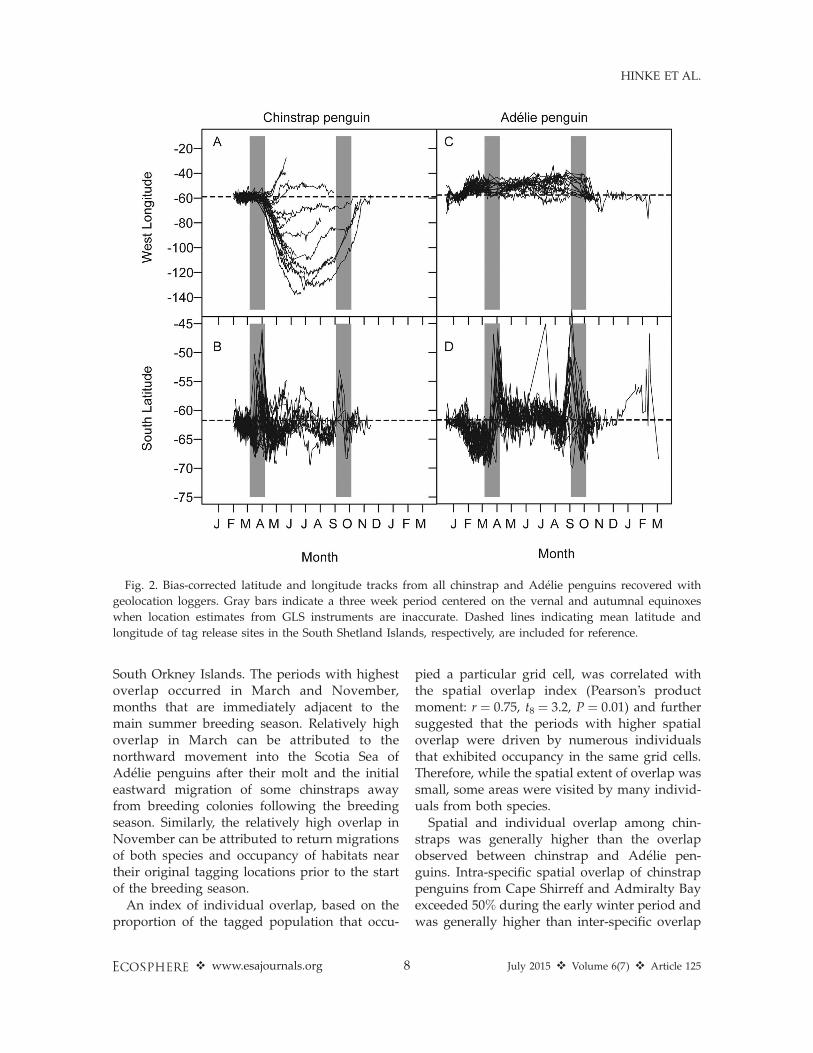
South Orkney Islands. The periods with highestoverlap occurred in March and November,months that are immediately adjacent to themain summer breeding season. Relatively highoverlap in March can be attributed to thenorthward movement into the Scotia Sea ofAdelie penguins after their molt and the initialeastward migration of some chinstraps awayfrom breeding colonies following the breedingseason. Similarly, the relatively high overlap inNovember can be attributed to return migrationsof both species and occupancy of habitats neartheir original tagging locations prior to the startof the breeding season.

An index of individual overlap, based on theproportion of the tagged population that occu-

pied a particular grid cell, was correlated withthe spatial overlap index (Pearson’s productmoment: r ¼ 0.75, t8 ¼ 3.2, P ¼ 0.01) and furthersuggested that the periods with higher spatialoverlap were driven by numerous individualsthat exhibited occupancy in the same grid cells.Therefore, while the spatial extent of overlap wassmall, some areas were visited by many individ-uals from both species.

Spatial and individual overlap among chin-straps was generally higher than the overlapobserved between chinstrap and Adelie pen-guins. Intra-specific spatial overlap of chinstrappenguins from Cape Shirreff and Admiralty Bayexceeded 50% during the early winter period andwas generally higher than inter-specific overlap

Fig. 2. Bias-corrected latitude and longitude tracks from all chinstrap and Adelie penguins recovered with

geolocation loggers. Gray bars indicate a three week period centered on the vernal and autumnal equinoxes

when location estimates from GLS instruments are inaccurate. Dashed lines indicating mean latitude and

longitude of tag release sites in the South Shetland Islands, respectively, are included for reference.


HINKE ET AL.

Fig. 3. Representative habitat utilization during winter months for chinstrap and Adelie penguins in March,

May, July, and September. Isotherms for 28C and 38C and contours for 15% and 50% sea ice concentration are

plotted for reference. Maps for all winter months for each species are included in Appendix C.


HINKE ET AL.

throughout the winter (Fig. 4B). The relatively

high overlap during the early winter period

again suggested common migratory corridors for

chinstraps with minimal segregation of spatial

habitats based on natal colony. As winter

progressed a decline in overlap was observed

(Fig. 4B) that could be attributed to spatial

segregation as individuals chose foraging

grounds scattered across the wide range of

longitudes (Fig. 3).

Isotopic niche

Stable isotope values of tail feathers and the

extent of overlap in niche space differed between

and within species. Both d13C (F1,50¼ 46.01, P ,

0.01) and d15N (F1,50 ¼ 49.95, P , 0.01) differed

between species, with mean carbon and nitrogen

isotope values higher in chinstrap relative to

Adelie penguins (Table 2, Fig. 4C). Core and total

isotopic niche sizes were also larger in chinstrap

penguins compared to Adelie penguins (Table 2).

Generally, core isotopic niches overlapped little

Fig. 4. Indices of spatial overlap and stable isotopic signatures for (A) Spatial and individual indices of overlap

between Adelie and all chinstrap penguins. (B) Index of spatial overlap among chinstrap penguins from

Admiralty Bay and Cape Shirreff. (C) Stable isotope values with estimates of core (SEAc; ellipses) and total niche

areas (TA; convex polygons) for Adelie and all chinstrap penguins. (D) Stable isotope values with estimates of

core (SEAc; ellipses) and total niche areas (TA; convex polygons) for chinstrap penguins from Admiralty Bay and

Cape Shirreff.


HINKE ET AL.

Fig. 5. Maps of monthly joint probability of spatial overlap for Adelie and chinstrap penguins.


HINKE ET AL.

between Adelie and chinstrap penguins (0.0% ofcore niche area and 2.9–5.6% of individuals withthe core area; Fig. 4C), though there was a largerand more variable degree of overlap whenexamining total niche space (15.3–54.2% of totalarea and 8.8–44.4% of individuals within thetotal area; Fig. 4C). Within a species, however,chinstrap penguins from different breeding sitesexhibited no difference in mean tail-feather d13C(F1,32¼ 1.68, P¼ 0.20) and d15N (F1,32¼ 0.81, P¼0.37; Table 2, Fig. 4D). The niche areas ofchinstrap penguins from Admiralty Bay andCape Shirreff exhibited a higher degree ofoverlap in core niche space (54.2–87.7% of corearea and 40.0–47.4% of individuals within thecore area) and total niche space (64.7–73.8% oftotal area and 60.0–68.4% of individuals with thetotal area) between sites (Fig. 4D).

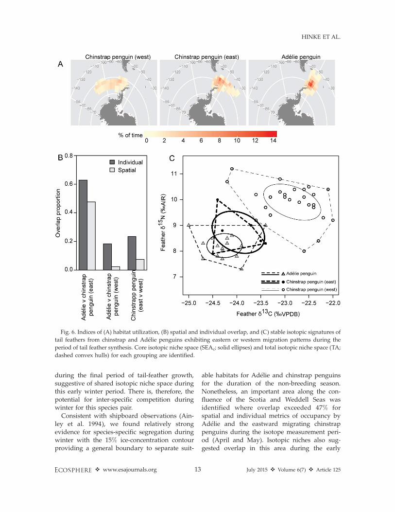
When GLS tracked penguins were divided byspecies and eastward vs. westward migrationpatterns (Fig. 6A), we found differences in spatialoverlap, isotopic values, and isotopic niche space.Spatial overlap during the period of feathergrowth was highest for Adelie penguins andthose chinstrap penguins that exhibited eastwardmigrations (Fig. 6B). The Adelie and eastwardmigrating chinstrap penguins had similar d13C(F1,22¼ 4.29, P¼ 0.05) and d15N (F1,22¼ 2.46, P¼0.13) values in their tail feathers while chinstrapsthat exhibited westward migration patterns haddifferent d13C (F1,50 ¼ 89.23, P . 0.01) and d15N(F1,50¼ 77.43, P . 0.01) tail-feather values relativeto all eastward moving birds (Fig. 6C). Corre-spondingly, Adelie and eastward migrating chin-strap penguins had a high degree of overlap incore niche space (19.0–49.4% of core area and16.7–22.2% of individuals within the core area)and total niche space (45.0–68.2% of total area

and 38.9–50.0% of individuals within the totalarea; Fig. 6C). Chinstrap penguins that exhibiteda westward migration pattern had lower isotopicoverlap (0.0% of core niche space and 0.0–3.6% ofindividuals) with eastward migrating penguins(Fig. 6C).

DISCUSSION

In this study we simultaneously tracked Adelieand chinstrap penguins from adjacent breedingcolonies during the austral winter. The area ofmarine habitat used by chinstrap and Adeliepenguins tagged from the South Shetland Islandswas expansive, covering over 1008 of longitude,and occupying a variable latitudinal rangebounded by advancing pack ice in the southand the 28C isotherm in the north. Such large-scale occupancy of marine habitats from twosmall seabird colonies in the South ShetlandIslands highlights the mobility of these penguinspecies and the general suitability of vastexpanses of the Southern Ocean pelagic regionas winter habitat for chinstrap and Adeliepenguins. The majority of observations indicatethat inter-specific overlap of habitat during thenon-breeding season is minimal, while intra-specific overlap by chinstraps from adjacentbreeding colonies was higher. These resultsindicate spatial segregation is the primary mech-anism of inter-specific niche separation duringwinter for Adelie and chinstrap penguins. How-ever, it is important to note that a pelagic corridoralong the confluence of the Weddell and ScotiaSeas was occupied by chinstrap and Adeliepenguins for most months of the year. Moreover,the eastward-migrating chinstrap and Adeliepenguins had similar stable isotope signatures

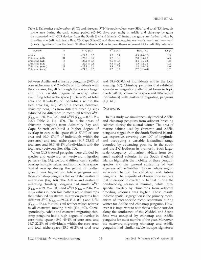
Table 2. Tail feather stable carbon (d13C) and nitrogen (d15N) isotopic values, core (SEAb) and total (TA) isotopic

niche area during the early winter period (40–100 days post molt) in Adelie and chinstrap penguins

instrumented with GLS devices from the South Shetland Islands. Chinstrap penguins are further divide by

breeding site (AB: Admiralty Bay; CS: Cape Shirreff ) and those undergoing eastwards (east) and westward

(west) migrations from the South Shetland Islands. Values in parentheses represent 95% credibility intervals.

Species N d13C (%) d15N (%) SEAb (%) TA (%)

Adelie 18 �24.3 6 0.3 8.2 6 0.4 0.9 (0.6–1.3) 1.9Chinstrap (all) 34 �23.0 6 0.7 9.7 6 0.8 2.0 (1.5–2.6) 6.5Chinstrap (AB) 15 �23.2 6 0.8 9.6 6 0.8 2.4 (1.6–3.8) 4.8Chinstrap (CS) 19 �22.9 6 0.6 9.8 6 0.8 1.5 (1.2–2.5) 4.2Chinstrap (west) 28 �22.8 6 0.6 9.9 6 0.7 1.4 (1.0–1.9) 4.0Chinstrap (east) 6 �24.0 6 0.5 8.7 6 0.7 2.2 (1.1–4.0) 1.2


HINKE ET AL.

during the final period of tail-feather growth,suggestive of shared isotopic niche space duringthis early winter period. There is, therefore, thepotential for inter-specific competition duringwinter for this species pair.

Consistent with shipboard observations (Ain-ley et al. 1994), we found relatively strongevidence for species-specific segregation duringwinter with the 15% ice-concentration contourproviding a general boundary to separate suit-

able habitats for Adelie and chinstrap penguinsfor the duration of the non-breeding season.Nonetheless, an important area along the con-fluence of the Scotia and Weddell Seas wasidentified where overlap exceeded 47% forspatial and individual metrics of occupancy byAdelie and the eastward migrating chinstrappenguins during the isotope measurement peri-od (April and May). Isotopic niches also sug-gested overlap in this area during the early

Fig. 6. Indices of (A) habitat utilization, (B) spatial and individual overlap, and (C) stable isotopic signatures of

tail feathers from chinstrap and Adelie penguins exhibiting eastern or western migration patterns during the

period of tail feather synthesis. Core isotopic niche space (SEAc; solid ellipses) and total isotopic niche space (TA;

dashed convex hulls) for each grouping are identified.


HINKE ET AL.

winter migration period. The spatial and isotopicoverlap observed during the early winter migra-tion period suggests the importance of thismarine habitat for both species. For example,post-molt mass of adult chinstrap penguins istypically 81% of typical mass during the breedingseason (US AMLR, unpublished data). Feedingconditions and the potential for competition forshared resources immediately following the moltmay therefore be critical for recovery of bodymass and, ultimately, survival.

Mechanisms that reinforce intra-specific spatialniche separation among Adelie penguins mayinclude colony-specific patterns in dispersal frombreeding colonies that help minimize overlapwith other breeding populations. We havetracked individuals from one small colony, butit is useful to compare their dispersal patternswith those from other studies. For example, datafrom Adelie penguins tracked from MargueriteBay, along the southwestern Antarctic Peninsula,demonstrate relatively local movements con-strained by the development and advection ofsea ice from the Bellingshausen Sea northwardalong the western Antarctic Peninsula (Erdmannet al. 2011); birds from the South Orkney Islandsexhibited larger-scale southward movements intothe Weddell Sea (Dunn et al. 2011); and Adeliepenguins from colonies in the Ross Sea and alongEast Antarctica must migrate north to themarginal ice zone and daylight during winter(Clarke et al. 2003, Ballard et al. 2010). AmongAdelie penguins, movement patterns appear tobe dictated by the location of a breeding colonyrelative to the advancing winter sea ice. Adeliepenguins from Admiralty Bay conform to thisgeneral model by first moving south into ice-covered areas in the Weddell Sea and thenmoving north as the ice edge advanced. Suchmigratory dependencies based on colony loca-tion relative to the nearest sea ice edge may helpmaintain colony or meta-population (Ainley et al.1995) segregation at sea for Adelie penguins.

Winter tracking studies of chinstrap penguinsare comparatively scarce, but two studies fromthe South Shetland Islands suggested a mixtureof movement patterns that include retention nearbreeding colonies during early winter versuslarger-scale (.1000 km), directed eastwardmovement toward the South Orkney and SouthSandwich Islands along the confluence of the

Scotia and Weddell seas (Wilson et al. 1998,Trivelpiece et al. 2007). We observed thesepatterns and add a third major pattern of large-scale westward movement into remote pelagicregions of the Bellingshausen and AmundsenSeas. The westward migration was the mostcommonly observed movement pattern of chin-strap penguins from Cape Shirreff (81% ofdeployments) and Admiralty Bay (63% of de-ployments). The large-scale westward movementchallenges the hypothesis forwarded by Trivel-piece et al. (2007) that proposed the mainmigratory directions exhibited by individualswas related to the location of ancestral sourcepopulations. The high degree of westwardmovement is therefore curious because thereare no major chinstrap colonies west of the SouthShetland Islands that could be a potential sourcepopulation. It is unknown if this westwardmovement pattern has developed since earliertracking studies were conducted or whetherprevious tracking studies from the South Shet-land Islands did not reveal this behavior becausesample sizes were small (Wilson et al. 1998,Trivelpiece et al. 2007). Of note, Ratcliffe et al.(2014) reported that the macaroni (Eudypteschrysolophus) and rockhopper (E. chrysocome)penguins tracked from South Georgia and theFalkland Islands exhibited high rates of occu-pancy in the Scotia Sea during winter. Thewestward movement of chinstrap penguins fromthe Peninsula region may, therefore, be a behav-ioral response to avoid high densities of theseEudyptes penguins in the central Scotia Sea.Regardless, it is clear that suitable winterforaging areas for chinstrap penguins from theAntarctic Peninsula region span a wide longitu-dinal range that includes the ice-free Pacificsector of the Southern Ocean.

Despite the widespread use of large swaths ofthe Southern Ocean, we do not find strongevidence for colony-specific spatial segregationduring winter. All chinstraps moved alongsimilar eastern or western corridors at similartimes and exhibited broad overlap in ice freepelagic areas throughout the winter. The reducedspatial overlap of chinstraps from differentcolonies that was estimated for mid-wintermonths can be partially attributed to selectionof different termination points for each individ-ual, rather than a colony-specific preference for


HINKE ET AL.

separate areas. For example, the tracking datademonstrate that individual differences existedin the rate of westward movement, selection ofover-winter foraging grounds, and commence-ment of return migration (Fig. 2). Such individ-ual-based selection results in a more diffusedistribution across wide swaths of suitable chin-strap habitat in the Southern Ocean that tends toreduce estimates of overlap. Alternatively, wenote that diminishing sample sizes as the numberof tag failures increased could also account forthe reduced overlap in mid-winter. Nonetheless,the observation of generally high winter overlapof birds from different breeding colonies sup-ports our original hypothesis that overlap ofchinstraps would occur, and provides a contrastwith recent studies on Eudyptes penguins. Thie-bot et al. (2011) reported fully distinct winterhabitats for macaroni penguins (E. chrysolophus)tracked from Crozet and Kerguelen Islands,colonies separated by 1400 km. Similarly, Rat-cliffe et al. (2014) demonstrated distinct winterforaging areas among southern rockhopperpenguins (E. chrysocome chrysocome) from colo-nies separated by 250 km on the FalklandIslands.

The above species-specific differences in spa-tial overlap during the non-breeding season maydepend on the size and proximity of the twobreeding populations considered. Ainley et al.(1995) hypothesized that adjacent colonies mayact more as a meta-population rather than a set ofstrictly independent breeding aggregations. Wenote that the two tagging locations for chinstrappenguins in this study were much closer (120km) than either of the other studies (.250 km).While foraging ranges of conspecifics fromadjacent colonies seldom overlap during thebreeding season (Wilson 2010), presumably dueto predictable aggregations of high-density preynear colony locations (Fraser and Trivelpiece1996), the relatively high degree of overlap ofchinstraps from our study sites during wintercorroborates this meta-population hypothesis.Specifically, the overlap facilitates contact andpotential mixing of individuals from multiplebreeding locales. We further suggest that thesmall and regionally declining breeding clustersof chinstrap penguins in the Antarctic Peninsularegion may be responding to large-scale drivers(Trivelpiece et al. 2011). The observation of

shared occupancy of wide swaths of the SouthernOcean during winter suggests a mechanism,namely shared winter habitats, by which ameta-population could exhibit similar long-termtrends across distinct breeding locations.

We identified a differentiation of isotopic nichespace from late-grown sections of tail feathersthat was correlated with the movement patternsof our study birds. This suggests that large-scalemigration patterns in Adelie and chinstrappenguins may be estimable from SIA of tailfeathers. However, linking animal movementpatterns with variation in tissue stable isotopevalues relies on an understanding of the timingof tissue synthesis and any possible lags betweenresource acquisition and mobilization for tissuegrowth (Bearhop et al. 2002, Martınez del Rio etal. 2009, Ramos and Gonzalez-Solıs 2012). None-theless, there are several lines of evidence tosupport our inference.

First, the captive growth study demonstratedthat tail feather growth is completed after themain body plumage molt (Appendix B). Second,while there is relatively less empirical dataavailable on the isotopic turn-over of feathers,turn-over rates of whole blood and feathersappear to be similar (Bearhop et al. 2002). Studiesof captive African penguins (Spheniscus demersus)indicate that whole blood integrates dietaryinformation over a period 20 days (Barquete etal. 2013), though turn-over rates are predicted tobe faster in wild birds due to higher metabolicrates (Bearhop et al. 2002). Using this conserva-tive 20-day window as a benchmark and thelikely timing of synthesis for tail feather sectionused in our analysis (59 6 11 and 69 6 20 daysafter the on-set of molt for chinstrap and Adeliepenguins, respectively), the earliest isotopicsignal observed in our data may therefore reflecta time period averaged from 38–59 days and 49–69 days after the onset of molt, respectively. Atthese times, the molt fast was over, migrations towinter foraging habitat were underway, andgeographic separation existed between birdsmoving mainly east or west. Finally, we notethat penguins are in the poorest body conditionof their annual cycle following the fast thataccompanies the body-plumage molt (Adamsand Brown 1990). Once the body molt iscomplete, the birds commence migrations towintering habitats, and resume feeding to recov-


HINKE ET AL.

er critical body reserves while at the same timecompleting tail feather growth. While we mustmake assumptions about mobilization of anyremaining body reserves versus routing of newconsumption to tail feather growth, severalobservations suggests that resource consumptionduring migration fuels tail feather synthesis.First, the diets of adult chinstrap and Adeliepenguins at the study colonies during thesummer breeding season are similar acrossindividuals, consistent over the course of thebreeding season, and similar year after year(Hinke et al. 2007). Second, isotope values fromfeathers grown in fledgling chicks (reflectingsummer diets provided by the adult) also exhibitvery low inter-individual variation (Cherel andHobson 2007, Polito et al. 2015). This leads to anexpectation that tail feather isotope values of allindividuals, particularly within a species fromthe same breeding locations, would be similar iffeather synthesis was dependent on pre-molt(summer) diets or body reserves. In contrast, weobserved different isotopic values from birdswith contrasting movement patterns, suggestingthat resource consumption during migrationfuels tail feather synthesis.

Although our sample sizes are relatively small,the degree of differentiation observed in theisotopic niche space among individuals migrat-ing into Pacific or Atlantic sectors of the SouthernOcean suggests that basin-scale differences in theisotopic composition of penguin prey resourcesare reflected in their tissues. The observeddifferences within and between species indicatesthat isotope signatures from penguin tail feathersmay be a useful tracer for identifying large-scalemovement patterns of Adelie and chinstrappenguins, similar to other Southern Oceanseabirds (e.g., Cherel and Hobson 2007, Phillipset al. 2009, Jaeger et al. 2010, Quillfeldt et al.2010). However, it is important to note thatconsumer stable isotope values can change overtime due to shifts in dietary composition ormovement between geographic location withdiffering isotopic baselines (e.g., Cherel andHobson 2007, Brasso and Polito 2013, McMahonet al. 2013). These factors make it difficult todetermine if the difference in isotopic niche spaceobserved between individuals migrating intoPacific or Atlantic sectors of the Southern Oceanmay arise from different diets, variation in

baseline stable isotopes values, or some combi-nation of the two. Studies using techniques thatcan differentiate between these two factors, suchas the compound specific-stable isotope analysisof amino acids, are advisable in the future(McMahon et al. 2013).

ConclusionsA goal of miniaturization of tagging technol-

ogies and isotopic study of body tissues, partic-ularly for migrating animals in marineenvironments, is to allow the identification offoraging locations without the need for expensiveand invasive sampling techniques. By integratinglight-based geolocation data and estimates ofisotopic niche from the analysis of 13C and 15Ncomposition of tail feathers, we revealed wide-spread use of the Southern Ocean by chinstrappenguins. The results suggest relatively broadintra-specific overlap of winter habitats for chin-strap penguins from two breeding colonies in theSouth Shetland Islands, in contrast with thelarge-scale spatial segregation of winter foraginghabitats used by Adelie and chinstrap penguins.However, the confluence of the Weddell andScotia Seas was an area in which both speciesexhibited consistent spatial and isotopic overlap.This confluence region represents a criticalcorridor for early winter movements and feedingconditions there may impact recovery of post-molt body mass and survival. Finally, theseparation of isotopic niche space that wascorrelated with the large-scale movement pat-terns suggests the ability to estimate basin-scalemovements of penguins on a population level vialarge-scale collection of feathers. Such popula-tion-level estimates of habitat use, while neces-sarily coarse in resolution, may provide novelmonitoring opportunities for these highly mobileseabirds in the future.

ACKNOWLEDGMENTS

We thank M. Mudge, N. Cook, M. Goh, S. Trivel-piece, P. Chilton, B. Soucie, M. Henschen, C. Bishop,and A. Bertoldi for assistance deploying and recover-ing tags for this study. Funds for the GLS tags wereprovided by the National Marine Sanctuary Founda-tion. Thank you also to S. Branch and the aviculturedepartment at SeaWorld Orlando for assistance inmeasuring penguin tail feather growth rates. Addi-tional support for this project was provided by a


HINKE ET AL.

Woods Hole Oceanographic Devonshire Scholarship aswell as funding from the Ocean Life Institute andSeaWorld Bush Gardens Conservation Fund to MJP.Reference to any specific commercial products, pro-cess, or service by trade name, trademark, manufac-turer, or otherwise, does not constitute or imply itsrecommendation, or favoring by the United StatesGovernment or NOAA/National Marine FisheriesService. Use of information from this publication shallnot be used for advertising or product endorsementpurposes. The Antarctic fur seal portion of this study(mobile control tags) was conducted under the MarineMammal Protection Act Permit #16472-01. All proto-cols were reviewed and approved by the UCSDIACUC.

LITERATURE CITED

Adams, N. J., and C. R. Brown. 1990. Energetics ofmolt. Pages 297–315 in L. S. Davis and J. T. Darby,editors. Penguin biology. Academic Press, SanDiego, California, USA.

Ainley, D. G., N. Nur, and E. J. Woehler. 1995. Factorsaffecting the distribution and size of Pygoscelidpenguin colonies in the Antarctic. Auk 112:171–182.

Ainley, D. G., C. A. Ribic, and W. R. Fraser. 1994.Ecological structure among migrant and residentseabirds of the Scotia-Weddell confluence region.Journal of Animal Ecology 63:347–364.

Ballard, G., V. Toniolo, D. G. Ainley, C. L. Parkinson,K. R. Arrigo, and P. N. Trathan. 2010. Respondingto climate change: Adelie penguins confrontastronomical and ocean boundaries. Ecology91:2056–2069.

Barquete, V., V. Strauss, and P. G. Ryan. 2013. Stableisotope turnover in blood and claws: a case studyin captive African Penguins. Journal of Experimen-tal Marine Biology and Ecology 448:121–127.

Bearhop, S., S. Waldron, S. C. Votier, and R. W.Furness. 2002. Factors that influence assimilationrates and fractionation of nitrogen and carbonstable isotopes in avian blood and feathers.Physiological and Biochemical Zoology 75:451–458.

Biuw, M., C. Lydersen, P. J. Nico de Bruyn, A. Arriola,G. G. J. Hofmeyr, P. Kritzinger, and K. M. Kovacs.2010. Long-range migration of a chinstrap penguinfrom Bouvetøya to Montagu Island, South Sand-wich Islands. Antarctic Science 22:157–162.

Block, B. A., et al. 2011. Tracking apex marine predatormovements in a dynamic ocean. Nature 475:86–90.

Bodey, T. W., E. J. Ward, R. A. Phillips, R. A. McGill,and S. Bearhop. 2013. Species versus guild leveldifferentiation revealed across the annual cycle byisotopic niche examination. Journal of AnimalEcology 83:470–478.

Bond, A. L., and L. L. Jones. 2009. A practicalintroduction to stable-isotope analysis for seabirdbiologists: approaches, cautions and caveats. Ma-rine Ornithology 37:183–188.

Bost, C. A., J. B. Charrassin, Y. Clerquin, Y. Ropert-Coudert, and Y. Le Maho. 2004. Exploitation ofdistant marginal ice zones by king penguins duringwinter. Marine Ecology Progress Series 283:293–297.

Brasso, R. L., and M. J. Polito. 2013. Trophic calcula-tions reveal the mechanism of population-levelvariation in mercury concentrations between ma-rine ecosystems: case studies of two polar seabirds.Marine Pollution Bulletin 75:244–249.

Cherel, Y., and K. A. Hobson. 2007. Geographicalvariation in carbon stable isotope signatures ofmarine predators: a tool to investigate theirforaging areas in the Southern Ocean. MarineEcology Progress Series 329:281–287.

Cherel, Y., M. Le Corre, S. Jaquemet, F. Menard, P.Richard, and H. Weimerskirch. 2008. Resourcepartitioning within a tropical seabird community:new information from stable isotopes. MarineEcology Progress Series 366:281–291.

Clarke, J., K. Kerry, C. Fowler, R. Lawless, S. Eberhard,and R. Murphy. 2003. Post-fledging and wintermigration of Adelie penguins Pygoscelis adeliae inthe Mawson region of East Antarctica. MarineEcology Progress Series 248:267–278.

Connan, M., C. D. McQuaid, B. T. Bonnevie, M. J.Smale, and Y. Cherel. 2014. Combined stomachcontent, lipid and stable isotope analyses revealspatial and trophic partitioning among threesympatric albatrosses from the Southern Ocean.Marine Ecology Progress Series 497:259–272.

Croxall, J. P., P. A. Prince, and K. Reid. 1997. Dietarysegregation of krill-eating South Georgia seabirds.Journal of Zoology 242:531–556.

Dunn, M. J., J. R. D. Silk, and P. N. Trathan. 2011. Post-breeding dispersal of Adelie penguins (Pygoscelisadeliae) nesting at Signy Island, South OrkneyIslands. Polar Biology 34:205–214.

Ekstrom, P. A. 2004. An advance in geolocation bylight. Memoirs of the National Institute of PolarResearch, Special Issue 58:210–226.

Erdmann, E. S., C. A. Ribic, D. L. Patterson-Fraser, andW. R. Fraser. 2011. Characterization of winterforaging locations of Adelie penguins along theWestern Antarctic Peninsula, 2001-2002. Deep SeaResearch II 58:1710–1718.

Fraser, W. R., and W. Z. Trivelpiece. 1996. Factorscontrolling the distribution of seabirds: winter-summer heterogeneity in the distribution of Adeliepenguin populations. Pages 257–272 in R. M. Ross,E. E. Hofmann, and L. B. Quetin, editors. Founda-tions for ecological research west of the AntarcticPeninsula. American Geophysical Union, Washing-


HINKE ET AL.

ton, D.C., USA.Freitas, C., C. Lydersen, R. A. Ims, M. A. Fedak, and

K. M. Kovacs. 2008. A simple new algorithm tofilter marine mammal Argos locations. MarineMammal Science 24:315–325.

Gonzalez-Solıs, J., J. P. Croxall, D. Oro, and X. Ruiz.2007. Trans-equatorial migration and mixing in thewintering areas of a pelagic seabird. Frontiers inEcology and the Environment 5:297–301.

Hammerschlag-Peyer, C. M., L. A. Yeager, S. M.Araujo, and C. A. Layman. 2011. A hypothesis-testing framework for studies investigating onto-genetic niche shifts using stable isotope ratios.PLoS ONE 6:e27104.

Hinke, J. T., K. Salwicka, S. G. Trivelpiece, G. M.Watters, and W. Z. Trivelpiece. 2007. Divergentresponses of Pygoscelis penguins reveal a commonenvironmental driver. Oecologia 153:845–855.

Hinke, J. T., S. G. Trivelpiece, and W. Z. Trivelpiece.2014. Adelie penguin (Pygoscelis adeliae) survivalrates and their relationship to environmentalindices in the South Shetland Islands, Antarctica.Polar Biology 37:1797–1809.

Hobson, K. A. 1999. Tracing origins and migration ofwildlife using stable isotopes: a review. Oecologia120:314–326.

Hutchinson, G. E. 1959. Homage to Santa Rosalia, orwhy are there so many kinds of animals? AmericanNaturalist 93:145–159.

Inger, R., and S. Bearhop. 2008. Applications of stableisotope analyses to avian ecology. Ibis 150:447–461.

Jackson, A. L., R. Inger, C. A. Parnell, and S. Bearhop.2011. Comparing isotopic niche widths among andwithin communities: SIBER–Stable Isotope Bayes-ian Ellipses in R. Journal of Animal Ecology80:595–602.

Jaeger, A., V. J. Lecomte, H. Weimerskirch, P. Richard,and Y. Cherel. 2010. Seabird satellite trackingvalidates the use of latitudinal isoscapes to depictpredators’ foraging areas in the Southern Ocean.Rapid Communications in Mass Spectrometry24:3456–3460.

Johnson, D., J. London, M.-A. Lea, and J. Durban. 2008.Continuous-time correlated random walk modelfor animal telemetry data. Ecology 89:1208–1215.

Karnovsky, N., D. G. Ainley, and P. Lee. 2007. Theimpact and importance of production in polynyasto top trophic predators: three case studies. Pages391–410 in W. O. Smith, Jr. and D. G. Barber,editors. Polynyas: windows to the world. Elsevier,Amsterdam, The Netherlands.

Kooyman, G. L., E. C. Hunke, S. F. Ackley, R. P. vanDam, and G. Robertson. 2000. Moult of theemperor penguin: travel, location, and habitatselection. Marine Ecology Progress Series 204:269–277.

Layman, C. A., D. A. Arrington, C. G. Montana, and

D. M. Post. 2007. Can stable isotope ratios providefor community-wide measures of trophic struc-ture? Ecology 88:42–48.

Lewis, S., T. N. Sherratt, K. C. Hamer, and S. Wanless.2001. Evidence of intra-specific competition forfood in a pelagic seabird. Nature 412:816–819.

Lynch, H. J., R. Naveen, P. N. Trathan, and W. F. Fagan.2012. Spatially integrated assessments reveal wide-spread changes in penguin populations on theAntarctic Peninsula. Ecology 93:1367–1377.

Martınez del Rio, C., N. Wolf, S. A. Carleton, and L. Z.Gannes. 2009. Isotopic ecology ten years after a callfor more laboratory experiments. Biological Re-views 84:91–111.

Masello, J. F., R. Mundry, M. Poisbleau, L. Demongin,C. C. Voigt, M. Wikelski, and P. Quillfeldt. 2010.Diving seabirds share foraging space and timewithin and among species. Ecosphere 1:19.

McMahon, K. W., L. L. Hamady, and S. R. Thorrold.2013. A review of ecogeochemistry approaches toestimating movements of marine animals. Limnol-ogy and Oceanography 58:697–714.

Newsome, S. D., C. Martınez del Rio, S. Bearhop, andD. L. Phillips. 2007. A niche for isotopic ecology.Frontiers in Ecology and the Environment 5:429–436.

Phillips, R. A., S. Bearhop, R. A. R. McGill, and D. A.Dawson. 2009. Stable isotopes reveal individualvariation in migration strategies and habitatpreferences in a suite of seabirds during thenonbreeding period. Oecologia 160:795–806.

Phillips, R. A., J. R. D. Silk, J. P. Croxall, V. Afanasyev,and D. R. Briggs. 2004. Accuracy of geolocationestimates for flying seabirds. Marine EcologyProgress Series 266:265–272.

Polito, M. J., H. J. Lynch, R. Naveen, and S. D. Emslie.2011a. Stable isotopes reveal regional heterogeneityin the pre-breeding distributions and diets ofsympatrically breeding Pygoscelis spp. penguins.Marine Ecology Progress Series 421:265–277.

Polito, M. J., S. Abel, C. R. Tobias, and S. D. Emslie.2011b. Dietary isotopic discrimination in gentoopenguin (Pygoscelis papua) feathers. Polar Biology34:1057–1063.

Polito, M. J., W. Z. Trivelpiece, W. P. Patterson, N. J.Karnovsky, C. S. Reiss, and S. D. Emslie. 2015.Contrasting specialist and generalist patterns facil-itate foraging niche partitioning in sympatricpopulations of Pygoscelis penguins. Marine EcologyProgress Series 519:221–237.

Quillfeldt, P., J. F. Masello, R. A. McGill, M. Adams,and R. W. Furness. 2010. Moving polewards inwinter: A recent change in the migratory strategyof a pelagic seabird? Frontiers in Zoology 7:15.

Quillfeldt, P., J. F. Masello, J. Navarro, and R. A.Phillips. 2012. Year-round distribution suggestsspatial segregation of two small petrel species in


HINKE ET AL.

the South Atlantic. Journal of Biogeography40:430–441.

R Core Team. 2012. R: A language and environmentfor statistical computing. R Foundation for Statis-tical Computing, Vienna, Austria.

Ramos, R., and J. Gonzalez-Solıs. 2012. Trace me if youcan: the use of intrinsic biogeochemical markers inmarine top predators. Frontiers in Ecology and theEnvironment 10:258–266.

Ratcliffe, N., S. Crofts, R. Brown, A. M. M. Baylis, S.Adlard, C. Horswill, H. Venables, P. Taylor, P. N.Trathan, and I. J. Staniland. 2014. Love thyneighbor or opposites attract? Patterns of spatialsegregation and association among crested pen-guin populations during winter. Journal of Bioge-ography 41:1183–1192.

Reynolds, R. W., N. A. Rayner, T. M. Smith, D. C.Stokes, and W. Wang. 2002. An improved in situand satellite SST analysis for climate. Journal ofClimate 15:1609–1625.

Ricklefs, R. E. 1967. A graphical method of fittingequations to growth curves. Ecology 48:978–983.

Ricklefs, R. E., and G. L. Miller. 1999. Ecology. Fourthedition. W.H. Freeman, New York, New York,USA.

SAS Institute. 1999. SAS/GRAPH software: reference.Version 8. SAS Institute, Cary, North Carolina,USA.

Schoener, T. W. 1970. Non-synchronous spatial overlapof lizards in patchy habitats. Ecology 51:408–418.

Seminoff, J. A., S. R. Benson, K. E. Arthur, T. Eguchi,P. H. Dutton, R. F. Tapilatu, and B. N. Popp. 2012.Stable isotope tracking of endangered sea turtles:validation with satellite telemetry and d15N analy-sis of amino acids. PLoS ONE 7:e37403.

Shaffer, S. A., Y. Tremblay, H. Weimerskirch, D. Scott,D. R. Thompson, P. M. Sagar, H. Moller, G. A.

Taylor, D. G. Foley, B. A. Block, and D. P. Costa.2006. Migratory shearwaters integrate oceanicresources across the Pacific Ocean in an endlesssummer. Proceedings of the National Academy ofSciences USA 103:12799–12802.

Thiebot, J.-B., Y. Cherel, P. N. Trathan, and C.-A. Bost.2011. Inter-population segregation in winteringareas of macaroni penguins. Marine EcologyProgress Series 421:279–290.

Thiebot, J.-B., Y. Cherel, P. N. Trathan, and C.-A. Bost.2012. Coexistence of oceanic predators on winter-ing areas explained by population-scale foragingsegregation in space or time. Ecology 93:122–130.

Trivelpiece, W. Z., S. Buckelew, C. S. Reiss, and S. G.Trivelpiece. 2007. The overwinter distribution ofchinstrap penguins from two breeding sites in theSouth Shetland Islands of Antarctica. Polar Biology30:1231–1237.

Trivelpiece, W. Z., J. T. Hinke, A. K. Miller, C. S. Reiss,S. G. Trivelpiece, and G. M. Watters. 2011.Variability in krill biomass links harvesting andclimate warming to penguin population changes inAntarctica. Proceedings of the National Academyof Sciences USA 108:7625–7628.

Wilson, R. P. 2010. Resource partitioning and nichehyper-volume overlap in free-living Pygoscelidpenguins. Functional Ecology 24:646–657.

Wilson, R. P., B. M. Culik, P. Kosiorek, and D. Adelung.1998. The overwinter movement of a chinstrappenguin (Pygoscelis antarctica). Polar Record34:107–112.

Wilson, R. P., J. J. Ducamp, G. Rees, B. M. Culik, and K.Niekamp K. 1992. Estimation of location: globalcoverage sun light intensity. Pages 131–143 in I. M.Priede and S. M. Swift, editors. Wildlife telemetry:remote monitoring and tracking of animals. EllisHorward, Chichester, UK.

SUPPLEMENTAL MATERIAL

APPENDIX A

Summary of methods and results for the estimation

of bias and error in GLS data

Estimating error (bias and precision) in loca-

tion estimates is central to any animal tracking

study. A basic approach for such analyses

includes the deployment of control tags to

provide coordinates for known locations over

time that can be used estimate bias corrections

for raw data and provide estimates of precision

for input into state-space models that are used to

estimate migratory tracks of study animals. As

part of our research using light-based geolocation

tags (GLS) to study overwinter dispersal of

Antarctic fur seals and penguins from two long-


HINKE ET AL.

term monitoring sites in the South ShetlandIslands, we deployed two GLS tags (LotekNano-Lat 2900-series archival geolocation tags)on a stationary platform at Cape Shirreff, Living-ston Island (62.46248 S, 60.79168 W) during thewinters of 2011 and 2012 to monitor locationestimation error at a fixed location. We alsodeployed 2 GLS tags on Antarctic fur sealsalready instrumented with SPOT5 satellite tagsthat were tracked via the ARGOS system duringthe winter for 2011. These mobile ‘‘control’’ tagswere used to monitor error in GLS locationestimates across a range of southern hemispherelatitudes and to assess whether bias and preci-sion in the GLS data were independent oflocation.

For the purposes of the analysis using themobile control tags, we assumed that a meandaily locations from ARGOS positions, calculatedfrom all unique coordinates that had locationquality codes 3 through A, provided sufficientprecision to be classified as a known locationwith respect to the lower precision (;180 km)inherent in light-based geolocation estimates(Phillips et al. 2004). We also note that the fourcontrol tags were from different product batches,but onboard algorithms for estimating positionwere identical in all tags (P. O’Flaherty, personalcommunication).

Due to GLS tag failures during deployment,known errors in GLS location estimates duringequinox periods (Wilson et al. 1992), impossiblelocation estimates that were reported by the tags(latitudes .908 N or S and/or longitudes beyond1808 W or E), highly unlikely location estimates(any northern hemisphere locations), data points

deemed impossible based on a speed filter(Freitas et al. 2008), and a loss of potential datapoints due to non-overlap of ARGOS and GLSpositions estimates for mobile controls, only 46%of the original daily coverage provided by theGLS data was available for this analysis (TableA1). Note that we used a maximum sustainedspeed of 3 m�s�1 to filter the control tag data forimpossible points. This relatively high speed wasused to retain as many data points as possiblefrom the limited availability of control tag data.After filtering, the data set contained at least one(5.36 6 3.2; mean 6 SD) location estimate for allweeks of the year except for week 8 (19 Feb–25Feb), 13 (26 Mar–1 Apr), 30 (23 Jul–29 Jul), and37–38 (10 Sep–23 Sep) when no GLS estimates ofposition were available.

Bias estimationFor each available location estimate from the

GLS tags, we calculated the distance to itscorresponding known daily location along lati-tude and longitude lines. These daily estimates ofbias were then aggregated by week to calculate aweekly mean bias from the correspondingknown location. We acknowledge that mobiletags may have extensive movement during thecourse of one week, but limited data availabilityfrom the mobile tags necessitated this aggrega-tion. With the weekly mean latitudinal andlongitudinal bias from each tag, we calculated aweekly weighted-average bias across all tags,with the weighting based on the number of dailylocation estimates contributed by each tag. Thistime series of weighted averages was then fittedwith a smoothing spline to estimate the weekly

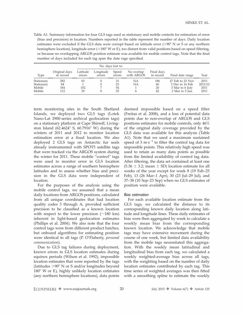
Table A1. Summary information for four GLS tags used as stationary and mobile controls for estimation of error

(bias and precision) in location. Numbers reported in the table represent the number of days. Daily location

estimates were excluded if the GLS data were corrupt based on latitude error (.908 N or S or any northern

hemisphere location), longitude error (.1808 Wor E), too distant from valid positions based on speed filtering,

or because no overlapping ARGOS position estimate was available for mobile control tags. Note that the final

number of days included for each tag span the date rage specified.

TypeOriginal days

in record

No. days lost to:

Final daysin record Final date range Year

Latitudeerrors

Longitudeerrors

Speederrors

No overlapwith ARGOS

Stationary 282 65 0 31 NA 186 27 Feb to 23 Nov 2011Stationary 84 1 0 23 NA 60 3 Dec to 16 Feb 2011/12Mobile 184 102 7 54 1 20 3 Mar to 6 July 2011Mobile 112 29 0 35 6 42 3 Mar to 5 Jun 2011


HINKE ET AL.

bias during the full year, including the 5 weekswith missing data. We used a loess smoother,implemented in R (R Core Team 2012), with span¼ 0.3 and degree ¼ 2.0. The weekly estimates oflatitudinal and longitudinal bias from thesmoothing spline were then used to correct the

raw GLS data from all tracked animals.The control-tag data identified a strong bias in

latitude estimates during the austral winter, withGLS location estimates typically 400–600 kmfurther north than known locations (Table A2,Fig. A1). The latitude bias was much reducedduring the austral summer, with GLS locationestimates typically within 200 km of knownlocations. Bias in longitude was smaller (gener-ally ,100 km) than for latitude, and exhibited noseasonal cycle (Table A2, Fig. A1.

Precision estimationTo estimate precision in the GLS locations, we

used a two-step approach. First, we calculated aweighted variance, as described above for theweekly bias estimation, for the weekly estimatesof latitudinal and longitudinal bias to representthe uncertainty in the raw GLS estimates oflocation. Second, we included uncertainty inposition estimates introduced as a result of thebias correction by implementing a bootstrapapproach. For the bootstrap procedure, wepooled the raw location estimates from all tags,randomly sub-sampled 75% of pooled data,reassigned the resulting data back to theirrespective tags, and repeated the weekly biascorrection estimation procedure for the each tagoutlined above. We repeated this process 10000times (Fig. A3). From the resulting collection ofsmoothed bias corrections, we calculated thevariance in the bias correction for latitude andlongitude for each week. The variances estimatedin steps 1 and 2 were added to estimate the totalvariance, and a square root was taken to estimatethe weekly standard deviation of location preci-sion. We then fitted a smoothing spline to thetime series of standard deviations of locationerrors as a final estimate of weekly error inlatitude and longitude position estimates for allweeks of the year, including those where no datawere available.

The weekly estimates of error in latitudesuggested that, on average, latitude error wasrough1y 1–28 (;111–222 km) while longitudeerror mainly ranged from 18 to 38 (;55–166 km)at these southern locales (assuming a latitude of608 S). We used these upper bounds on latitude(28) and longitude error (38) to define grid cellsizes for mapping habitat utilization.

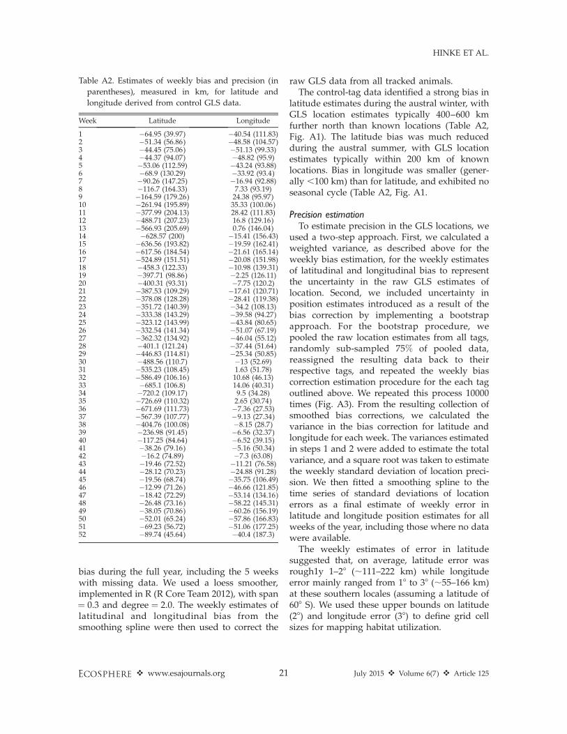
Table A2. Estimates of weekly bias and precision (in

parentheses), measured in km, for latitude and

longitude derived from control GLS data.

Week Latitude Longitude

1 �64.95 (39.97) �40.54 (111.83)2 �51.34 (56.86) �48.58 (104.57)3 �44.45 (75.06) �51.13 (99.33)4 �44.37 (94.07) �48.82 (95.9)5 �53.06 (112.59) �43.24 (93.88)6 �68.9 (130.29) �33.92 (93.4)7 �90.26 (147.25) �16.94 (92.88)8 �116.7 (164.33) 7.33 (93.19)9 �164.59 (179.26) 24.38 (95.97)10 �261.94 (195.89) 35.33 (100.06)11 �377.99 (204.13) 28.42 (111.83)12 �488.71 (207.23) 16.8 (129.16)13 �566.93 (205.69) 0.76 (146.04)14 �628.57 (200) �15.41 (156.43)15 �636.56 (193.82) �19.59 (162.41)16 �617.56 (184.54) �21.61 (165.14)17 �524.89 (151.51) �20.08 (151.98)18 �458.3 (122.33) �10.98 (139.31)19 �397.71 (98.86) �2.25 (126.11)20 �400.31 (93.31) �7.75 (120.2)21 �387.53 (109.29) �17.61 (120.71)22 �378.08 (128.28) �28.41 (119.38)23 �351.72 (140.39) �34.2 (108.13)24 �333.38 (143.29) �39.58 (94.27)25 �323.12 (143.99) �43.84 (80.65)26 �332.54 (141.34) �51.07 (67.19)27 �362.32 (134.92) �46.04 (55.12)28 �401.1 (121.24) �37.44 (51.64)29 �446.83 (114.81) �25.34 (50.85)30 �488.56 (110.7) �13 (52.69)31 �535.23 (108.45) 1.63 (51.78)32 �586.49 (106.16) 10.68 (46.13)33 �685.1 (106.8) 14.06 (40.31)34 �720.2 (109.17) 9.5 (34.28)35 �726.69 (110.32) 2.65 (30.74)36 �671.69 (111.73) �7.36 (27.53)37 �567.39 (107.77) �9.13 (27.34)38 �404.76 (100.08) �8.15 (28.7)39 �236.98 (91.45) �6.56 (32.37)40 �117.25 (84.64) �6.52 (39.15)41 �38.26 (79.16) �5.16 (50.34)42 �16.2 (74.89) �7.3 (63.08)43 �19.46 (72.52) �11.21 (76.58)44 �28.12 (70.23) �24.88 (91.28)45 �19.56 (68.74) �35.75 (106.49)46 �12.99 (71.26) �46.66 (121.85)47 �18.42 (72.29) �53.14 (134.16)48 �26.48 (73.16) �58.22 (145.31)49 �38.05 (70.86) �60.26 (156.19)50 �52.01 (65.24) �57.86 (166.83)51 �69.23 (56.72) �51.06 (177.25)52 �89.74 (45.64) �40.4 (187.3)


HINKE ET AL.

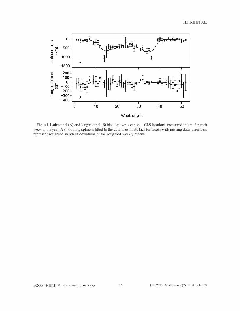
Fig. A1. Latitudinal (A) and longitudinal (B) bias (known location� GLS location), measured in km, for each

week of the year. A smoothing spline is fitted to the data to estimate bias for weeks with missing data. Error bars

represent weighted standard deviations of the weighted weekly means.


HINKE ET AL.

Fig. A2. Example of bias-corrected data for a stationary tag (A) and a mobile tag (B). (A) Raw GLS position

estimates (black dots), known location at Cape Shirreff, Livingston Island (red dot), and bias corrected location

estimates (blue dots). (B) ARGOS track line (solid black line), raw GLS track line (dashed red line) and bias-

corrected GLS track line (solid red line) for mobile GLS tag 0588.


HINKE ET AL.

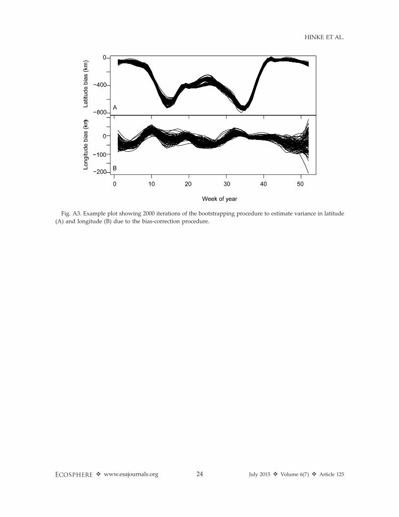
Fig. A3. Example plot showing 2000 iterations of the bootstrapping procedure to estimate variance in latitude

(A) and longitude (B) due to the bias-correction procedure.


HINKE ET AL.

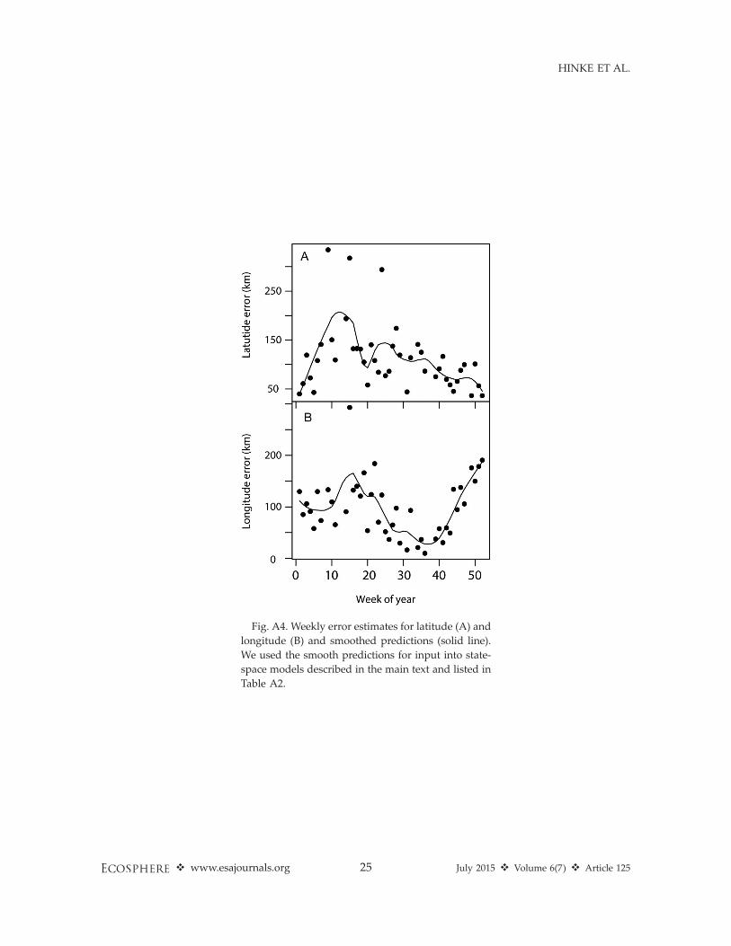
Fig. A4. Weekly error estimates for latitude (A) and

longitude (B) and smoothed predictions (solid line).

We used the smooth predictions for input into state-

space models described in the main text and listed in

Table A2.


HINKE ET AL.

APPENDIX B

Estimating the timing of tail-feather growthWe studied the growth of tail feathers in a

captive population of Adelie penguins main-tained at SeaWorld in Orlando, Florida, during2012. To estimate the timing and rate of feathergrowth, twelve individual adults (6 male and 6females) were monitored from the start of moltwhen flippers swell in size and old feathers beginto lift and stand out from the body. Following theonset of molt, the exposed length (cm) of thelargest newly growing central tail feather of eachindividual was measured at roughly 20-dayintervals until approximately 100 days after moltwhen growth of the tail feathers neared comple-tion. We assume that rate of feather synthesisand, hence, the duration of the feather growthperiod, is similar between captive and wildanimals. In support of this assumption wemeasured the exposed tail feather lengths in122 wild (King George and Livingston Islands,South Shetland Islands) and 44 captive (Sea-World) Pygoscelis penguins. Exposed tail featherdid not differ across all wild and captive specieseither following body molt completion (ANOVA:F3,71¼ 0.79, P¼ 0.50) when all feathers except thetail feathers are fully grown, nor outside of themolting period when tail feather are fully grown(ANOVA: F4,93 ¼ 2.30, P ¼ 0.07; Table B1). Inaddition, the duration of the body molt period issimilar between wild and captive Pygoscelispenguins (Adams and Brown 1990, Polito et al.2011b).

We note that the exposed length measurementdoes not account for the portion of each tailfeather found beneath the skin. To address thisdifference, we measured both the exposed lengthand total length of plucked tail feathers from asample of 19 Adelie (7 male and 12 female) and

33 chinstrap (19 male and 14 female) penguinsinstrumented with GLS tags at King George andLivingston Islands, South Shetland Islands. Meanhidden length (i.e., beneath the skin) of centraltail feathers did not differ between species (F1,52¼0.174, P¼ 0.678), sexes (F1,52¼ 0.1324, P¼ 0.572)or exhibit a significant interaction (F1,52¼ 0.188, P¼ 0.666). Therefore we added the overall meanhidden length (3.2 cm) across all species andsexes to our measurements of exposed tail featherlength and derived the total length of growingtail feathers measured in our captive study (TableB1). We then used PROC NLIN with theMarquardt method in SAS (SAS Institute 1999)to fit von Bertalanffy growth curves to thisdataset. The von Bertalanffy growth curve hasbeen commonly used to model growth in largeseabirds (Ricklefs 1967) and is formulated as:

Lt ¼ t‘

�1� e�kðt�t

0Þ�

where Lt is the predicted length (in cm) at time t(in days), L‘ is the mean length that would bereached if feathers grew indefinitely, k is agrowth parameter of dimension time�1, and t0is the hypothetical time (in days) when featherlength is zero. We modeled growth curvesseparately by sex and with both sexes combinedand compared 95% confidence intervals ofparameter estimates, residual mean square error(MSE) and pseudo-R2 as measures of goodnessof fit. Both MSE and pseudo-R2 indicated that thevon Bertalanffy growth curve fitted our data formales slightly better than for females and bothsexes combined, though 95% confidence intervals(CI) of parameter estimates overlapped substan-tially between all three models (Table B2). Due tothis overlap and the relatively small differencesbetween sexes we used the parameter estimatesderived from both sexes combined to estimate

Table B1. Comparison of exposed tail feather length immediately after the body molt is complete and outside of

the molt period in wild and captive penguins.

Group Species

Exposed tail feather at body molt completion Exposed fully grown tail feather

n Length (cm) n Length (cm)

Wild Adelie . . . . . . 18 15.5 6 1.2Chinstrap 20 2.0 6 0.7 34 14.6 6 1.2Gentoo 30 2.4 6 0.9 20 14.9 6 1.0

Captive Adelie 12 2.0 6 1.0 12 14.9 6 1.4Chinstrap . . . . . . . . . . . .Gentoo 10 2.2 6 0.8 10 14.5 6 1.2


HINKE ET AL.

Table B2. Parameter estimates, 95% confidence intervals (in parentheses), residual mean square error (MSE) and

pseudo-R2 values estimated from fitted von Bertalanffy growth equations of total feather length (cm) relative to

time (days) elapsed since the onset of feather molt.

Group

Parameter estimates Fit statistics

L‘ k t0 MSE Pseudo-R2

Males 19.5 (18.0–21.1) 0.03 (0.02–0.04) 7.8 (4.8–10.8) 0.765 0.968Female 18.3 (16.1–20.4) 0.03 (0.02–0.05) 8.2 (2.9–13.5) 2.6 0.877Combined 18.8 (17.5–20.2) 0.03 (0.02–0.04) 8.0 (4.9–11.1) 1.766 0.918

Table B3. Molt-timing information based on opportunistic observations of individuals at study colonies. All data

are unpublished US AMLR holdings.

Species Date Molt chronology How n

Chinstrap� 10 Feb (65 d) Initiation Observations of banded individuals molting 254Chinstrap� 19–27 Feb Completion Animals selected for overwinter tracking must be fully

molted for tag attachment30

Adelie� 10 Feb Initiation Observations of banded individuals molting 1Adelie 28 Feb Completion Animals selected for overwinter tracking must be fully

molted for tag attachment3

Adelie 11 Feb–11 Mar Initiation Loss of telemetry data due to presumed molt 4

� The opportunistically collected data on chinstraps reported here likely reflect timing for non-breeders and failed breedersand may be atypical of successful breeders. When annual research activities at Cape Shirreff end, typically in late February andearly March, aggregations of molting birds are still growing. Thus, we assume 1 March to be a more representative moltinitiation date for the majority of breeders despite the observational data suggesting otherwise.

� Observations of Adelie penguins molting on land in Admiralty Bay are rare.

Fig. B1. Fitted von Bertalanffy growth curve (solid line) and 95% confidence intervals (dotted lines) of total tail

feather length relative to time elapsed since the onset of feather molt in a captive population of twelve adult (6

male and 6 females) Adelie penguins maintained at SeaWorld in Orlando, Florida, during 2012.


HINKE ET AL.

the timing of tail feather synthesis based onlength (Fig. B1):

t ¼ t0 �1

k3 ln 1� Lt

L‘

� �

where t is the predicted time (in days) since thestart of molt that a section of tail feather at lengthLt was synthesized based on the predicted vonBertalanffy growth parameters (L‘ ¼ 18.832, k ¼0.031, t0 ¼ 8.035).

We applied the above formula to estimatetiming of growth for discrete sections of tailfeathers that were obtained from individualpenguins tracked with GLS instruments. Discretesections of the tail feathers were sampled forstable isotope analysis by using stainless steelscissors to cut a 0.5-cm section of feather shaft

from the proximal portion of each feather locatedjust above where the feather enters the skin.These mid-point of each section average 15.6 6

1.1 and 14.9 6 1.3 cm from the distal tip and thusrepresented growth occurring 69 6 20 (CI ¼ 42–110) and 59 6 11 (CI¼ 40–96) days following theonset of molt for Adelie and chinstrap penguins,respectively (i.e., 40–100 days following the onsetof molt). Given published (Dunn et al. 2011) andunpublished data on molt timing (Table B3) forAdelie and chinstrap penguins, we assume thatmolt initiation typically occurred on 14 Februaryfor Adelie penguins and 1 March for chinstrappenguins. Thus, the sampled feather sectionsreflect a time from late March to early June whenpenguins are migrating to and/or inhabiting theirover-wintering areas.

APPENDIX C

Monthly habitat utilization and distributions of surface temperature readings measuredby GLS tags deployed on chinstrap and Adelie penguins (see following pages)


HINKE ET AL.

Fig. C1. Monthly habitat utilization for chinstrap penguins during the non-breeding season.


HINKE ET AL.

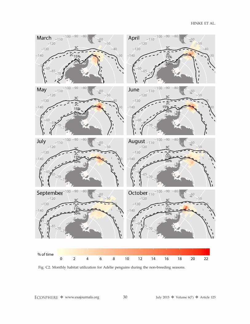
Fig. C2. Monthly habitat utilization for Adelie penguins during the non-breeding seasons.


HINKE ET AL.

Fig. C3. Monthly surface temperature distributions for chinstrap penguins. Data derive from once-daily

records of surface temperatures recorded by GLS tags, averaged over each month for each grid cell. Position

estimates used for this plot are bias-corrected, raw data.


HINKE ET AL.

Fig. C4. Monthly surface temperature distributions for Adelie penguins. Data derive from once-daily records of

surface temperatures recorded by GLS tags, averaged over each month for each grid cell. Position estimates used

for this plot are bias-corrected, raw data.


HINKE ET AL.

Documents

Spatial and isotopic niche partitioning during winter … · Spatial and isotopic niche partitioning during ... Spatial and isotopic niche partitioning during winter in chinstrap