Spatial Analysis of Infiltration Experiment - ajbasweb.comajbasweb.com/old/ajbas/2011/July-2011/729-742.pdf · Australian Journal of Basic and Applied ... Spatial Analysis of Infiltration

Australian Journal of Basic and Applied Sciences, 5(7): 729-742, 2011ISSN 1991-8178

Corresponding Author: Tarek Selim, Civil Engineering Department, Faculty of Engineering, Port Said University, Egypt

729

Spatial Analysis of Infiltration Experiment

1,2Tarek Selim, 2Ronny Berndtsson, 2Magnus Persson, 3Fethi Bouksila, 2Mohammad Aljaradin

1Civil Engineering Department, Faculty of Engineering, Port Said University, Egypt2Department of Water Resources Engineering, Lund University, Box 118, 221 00 Lund, Sweden

3INRGREF, B.P. 10, 2080 Ariana, Tunis el Menzah, Tunisia

Abstract: Developing correlations between various soil parameters are considered the major challengeto diminish time and cost associated with field measurements. Soil hydraulic and physical propertieswere extensively characterized using tension disc infiltrometer and soil sampling in a silty clayagricultural field in Kalaat El-Andalous, Tunisia. Tension disc infiltrometer experiments wereconducted at 109 plots with two supply water potentials (-30,-60 mm) at each plot to determine thehydraulic conductivity, sorptivity, capillary length, and matric flux potential. In addition, soil sampleswere analyzed to determine the soil bulk density, and water content. From the statistical and spatialanalysis for the different parameters, it was found that the soil hydraulic parameters had largervariability than bulk density. Sorptivity, capillary length, matric flux potential, and bulk density hadlager variance with the distance between the plots. No correlation was found between bulk densityand the soil hydraulic parameters, nor could the soil hydraulic parameters be correlated to each other.

Key words: Tension disc infiltrometer; soil hydraulic parameters; Minitab; Geoeas; Tunisia.

1. INTRODUCTION

One option for coping with the inaccurate estimation of crop requirements and the potential forgroundwater contamination from numerical simulation is the deterministic estimation of soil hydraulicproperties. Water retention and hydraulic conductivity curves are vital input data in any numerical simulationfor water flow and solute transport. In addition, the accurate determination of soil hydraulic parameters hada great effect on the susceptibility of the computed water balances (Jhorar et al., 2004).

The non-availability of hydraulic properties for most soils is the hindrance to be overcome for generalapplication of the numerical models (Messing and Jarvis,1993; Simunek et al.,1998). Laboratory experimentsare rooted in the adequate measurement of flow processes, but they are generally carried out on small soilsamples that lead to many questions about their validity in representation the field conditions. One reason forthe uncertainty of laboratory method results is the difficulty to capture the existence of stones, cracks, fissures,natural soil pipes, root holes, and fractures in unsaturated soil profiles in small-scale laboratory samples. Onthe other hand, inverse modeling had provided an alternative method for determining the hydraulic propertiesinstead of direct measurements but future improvement could still be needed (Abbaspour et al., 2001; Nemeset al., 2003; Ungaro et al., 2005).

Another different approaches for predicting soil hydraulic properties has been developed during the lastdecade like artificial neural networks (Minasny and McBratney, 2002; Schaap et al., 2001), vector machines(Lamorski et al., 2008), and non-parametric pattern recognition tools (Nemes et al., 2006c). Baroni et al.(2010) employed five direct and indirect methods to determine soil hydraulic parameters, two methods werebased on laboratory and field measurements, remaining three methods were based on the application of widelyused Pedo-Transfer Functions Rawls and Brakensiek, HYPRES, and ROSETTA. They demonstrated that a greatdifference of soil hydraulic parameter values generated with the direct and indirect methods, especially for thesaturated hydraulic conductivity and the shape parameter of the van Genuchten curve.

According to the aforementioned methods, although the difficulty of managing and controlling the fieldmethods, the in situ experiments are still the most confidence and robust method for determining theparameters that describe the soil hydraulic properties. Tension disc infiltrometer is a commonly method forsteady state field measurement of the unsaturated soil hydraulic conductivity at potential head close tosaturation (Perroux and White, 1988; Ankeny et al., 1991; Reynolds and Elrick, 1991; Logsdon and Jaynes,1993; Angulo-Jaramillo et al., 2000). Moreover, it used for quantifying the effects of macropores and

Aust. J. Basic & Appl. Sci., 5(7): 729-742, 2011

730

preferential flow paths on infiltration. Measurements of the contribution of macropores to the overall infiltrationcan be obtained by comparing infiltration rates during ponded conditions (Villholth et al., 1998).

Tension disc infiltrometer is a device used in both laboratory and field to illustrate water entry into thesoil under different negative water potential; the water flow through very small pores at large negative pressurehead. In Laboratory, Clothier et al. (1992) estimated the mobile and immobile water fractions depending onknowledge of the steady state water and solute distributions. Also Quardi et al. (1994) validated their finitedifference model for axisymmeteric water flow and solute transport using the same experimental set up.

Tension infiltrometer was used in field to determine the near saturated hydraulic conductivity by Messinget al. (1995) in six tilled soils of contrasting texture ranging from loamy sand to silty clay under supplypressure heads ranged from negative100 mm up to zero. They concluded that the near saturated hydraulicconductivity increased by three to four orders of magnitude in the finer textured soils and by about two ordersof magnitude in two sandy soils. Angulo-Jaramillo et al. (1997) used the tension disc infiltrometer to estimatethe unsaturated hydraulic conductivity in two different soils under conventional tillage and different irrigationpractices. They noted that the sandy soil under furrow irrigation showed a significant decrease in its hydraulicproperties with an increase in the bulk density. In addition, strong nonlinearity in the hydraulic conductivitywas found for the stony soil. Finally, they concluded that a good understanding of the porous network couldbe obtained from tension infiltrometers.

IRNASs and IAV (2000) participated in a joint experiment in the experimental site Saboun, Morocco. Thehydraulic conductivity and sorptivity were measured in the range near saturation by a tension disc infiltrometer.The water potentials applied in the experiments were -120, -80, -30, and –5 mm. Four transects wereinvestigated resulting in 15 measuring points. High variability was found for both hydraulic conductivity andsorptivity. For hydraulic conductivity at water potential equal -5 mm, the mean was 0.043 and standarddeviation was 0.028. For sorptivity at same pressure, the mean was 0.339 and standard deviation was 0.114.

On the other hand, Bagarello et al. (2005) used the tension infiltrometer in sandy loam to evaluate theinfluence of pressure head sequence (ascending or descending) on the hydraulic conductivity (K0) value. Theyconcluded that the applied pressure head sequence did not affect significantly the relative variability of the K0.

Determining general correlations between various soil hydraulic parameters by mean of tension discinfiltrometer dose not appear to have caught researcher’s attention so far. Therefore, Comprehensive analysisof the soil hydraulic parameters using tension disc infiltrometer was conducted so that an attempt to reducethe field data required for numerical modeling could be done by establishing correlations between different soilhydraulic parameters. The aim of this work was to 1) Analyze the spatial variability of soil hydraulicparameters in an agricultural field soil in order to describe water flow properties and 2) Establish correlationsbetween different soil parameters.

2. MATERIALS AND METHODS

2.1 Theoretical Background:Zhang (1998) proposed several procedures for estimating soil hydraulic conductivity from the data of

tension disc infiltrometer. The combination of Wooding’s (1968) analytical solution for steady infiltration froma circular source and the unsaturated hydraulic conductivity function given by Gardner’s (1958) exponentialmodel, is the most commonly applied approach used to determine the soil hydraulic conductivity from thetension infiltrometer data.

The relation between unsaturated-saturated hydraulic conductivity given by Gardner as follows

K(ψ) = Ksat exp (αψ) (1)

Wooding's analytical solution for infiltration from a circular source with a constant pressure head at thesoil surface and with the unsaturated hydraulic conductivity is given by

Q(ψ) = π r2 K(ψ) { 1 + (4/ π rα )} (2)

By combining equation 1,2 one can get the following equation

Q(ψ) = π r2 Ksat exp (α ψ) { 1 + (4/ π rα )} (3)

Either multiple disc radii (Hussen and Warrick, 1993) or multiple potentials (Ankeny et al., 1991; Messing


731

and Jarvis, 1995) are required to analyze the tension disc infiltrometer data based on the previous equation.By using two different potentials ψ1, ψ2 equation (3) will be in the form of

Q(ψ1) = π r2 Ksat exp (α ψ1) { 1 + (4/ π rα )} (4)

Q(ψ2) = π r2 Ksat exp (α ψ2) { 1 + (4/ π rα )} (5)

From equations 4,5 (α) can be described as follows

α = (6)2 1

ln[Q( Q

Sorptivity (S) is a parameter that describes how well the soil absorbs water. There are many ways fordetermining sorptivity. The simplest method is by using Philip (1957) one-dimensional horizontal infiltrationequation:

S = I / (7)t

Eq. 7 is a simplified form of: I = S t½ + At + Bt1.5 (8)

The first term of eq. 8 on the right hand side dominates the flow for a brief time after initiation ofinfiltration (about 120 s) and thus sorptivity can be calculated using eq. 7 (Klute, 1986). White and Sully(1987) and Vandervaere et al. (2000) have described calculations for sorptivity and the relationship withhydraulic conductivity in more details.

Water in soil is subjected to capillary forces due to surface tension of the air-water interface and thecontact angle with the solid particles (Hillel, 1971). Large soil capillary length increases the available waterfor the plant roots. The macroscopic capillary length can be calculated according to White and Sully (1987)as follows

λc = { K(ψ0) - K(ψn)} * (9)

0

( )n

K d

According to Wooding the capillary length equation can be simplified to:

λc = α-1 (10)

Another parameter controlling the availability of water to the plant is the matrix flux potential (Øm); Itdescribes how well the soil particles attract water. Large matric flux potential will cause the water to stay inthe top layer of the soil where it is possible for the plants to reach it. Then, matric flux potential can be usedwhen estimating how much irrigation water is needed and is expressed as follows:

Øm = K(ψ) / α (11)

2.2 Area Description:The infiltration experiments were carried out during the period 27/2/2002 to 16/3/2002 at an agricultural

field in Kalaat El-Andalous. The experimental site is situated in lower Medjerdah Valley, which is locatedapproximately 40 km NW of Tunis, Tunisia. The Soil is classified as silty clay and the water table is locatedat about 1.5 m depth. The field was planted during most of the year and irrigated from the Medjerdah Riverlocated close to the field. Since the field had been in use for several years, the top soil layer was well mixed.The climate at the field site is Mediterranean, characterized by mild rainy winters and dry summers. Duringthe period of experiments, there were some short nightly rainfalls, each lasting for a few hours. Thetemperature varied from 11 to 15 Co with strong sun during the day.


732

2.3 Field Experiments:Tension disc infiltrometer experiments were conducted in 109 plots within Kalaat El-Andalous agricultural

area (Fig. 1). At each plot, two different potential -30,-60 mm were used. Although, a certain degree ofpacking was observed due to the compaction by tractor wheel traffic. No plots were located directly in atractor track. Before experiments, the soil surface was leveled without disturbing the soil structure. Localirrigation water was used for the experiments.

The infiltrometer disc had a diameter of 8 cm and covered with special filter membrane. In addition, athin layer of fine sand was placed on the soil surface underneath the infiltrometer to assure good contactbetween the infiltrometer disc and the soil. Perroux and White (1988) recommended applying a high-permeability material to the undisturbed soil surface to establish a complete hydraulic bond between the diskand the infiltration surface. Other studies (Close et al. ,1998; Bagarello et al., 2001) have shown that the useof the contact material affects the infiltration.

During the experiments, a transducer, connected to the top of the infiltrometer water reservoir to convertthe negative potential in the water reservoir to voltage. The measured voltage was recorded every five secondsby mean of data logger connected to the transducer. This procedure was done to observe if the negativepotential in the air pocket at the top of the water reservoir could be linearly related to the height of the waterin the reservoir. If so, it would be possible to monitor the infiltration using shorter time interval.

Fig. 1: The experimental area.

Each experiment was carried out until reaching steady state condition, which means that the infiltrationof water was constant. In each plot, two soil samples at depth (0-10 cm, and 10- 20 cm) were taken in theinfiltration area to analyze the water content in the wetted soil. In addition, samples for measuring the bulkdensity were taken adjacent to the plot at the same depths.


733

2.4 Statistical Properties:Statistical analyses using a statistical software program Minitab version 7.2 were conducted on hydraulic

conductivity, sorptivity, capillary length, matric flux potential, bulk density and water content. Minitabcalculated the mean value (x*), the trimmed mean (tr x*) (the mean value of data after ignoring the smallestand largest five percent of the reading), standard deviation (σ), and the standard error of the mean (se x*). Thestandard error of the mean was calculated to note if the mean value is reprehensive for a series of data. If thecalculated error is small compared to the mean value, it is possible to use the mean as a representative numberfor a whole series of data.

The last parameter calculated by Minitab was the first and third quartile, Q1 and Q3. Where the firstquartile is the number, at which 25% of all values are lower than that number. Similarly, the third quartile isthe number when 75% of all values are lower than that number.

3. RESULTS AND DISCUSSION

3.1 Hydraulic Properties: The data collected during the experiments were infiltration rate, which was manually observed from the

infiltrometer, and soil potential measurements from the data logger. An attempt was conducted to identify arelation between the data logger values and the manual reading. By mean of twelve plots(7,8,9,38,39,40,41,42,43,47,48, and 49).A regression equation with the following form was conducted tocalculate infiltration from the data logger readings.

Y = 934.38X + 883.12 (12)

Where, X is the mean voltage (mV) and Y is the manually observed infiltration depth (mm).Comparing the measured infiltration values with the calculated values from the regression equation. It was

noted that there was a large variability between the measured and calculated values. The variability wasprobably due to a too sensitive transducer that picked up the pressure change when a bubble reached thesurface in the water tower. Therefore, the regression equation cannot be used.

After a constant infiltration rate was reached, using Wooding's method, the saturated hydraulic conductivityand near saturated hydraulic conductivity were calculated. Sorptivity, capillary length, and matric flux potentialwere calculated according to the aforementioned equations in the previous section.

3.2 Statistical Analysis:Statistical results obtained from Mintab are shown in table 1. The higher values of sorptivity were

observed in plots 15 and 17 under both water potentials -30, -60 mm. This was probably due to an earlyceasing of the experiments which didn’t allowed to reach the steady state and made the infiltration to be high.These higher sorptivity values were replaced with the mean sorptivity value to minimize its influence on thestatistical analysis.

From the statistical analysis, it was observed that the standard error of the mean was small in comparisonto the mean value, which indicates a dense concentration of values around the mean value. An exception wasseen for the sorptivity. This was due to plots 15 and 17 had values up to 20 times larger than the mean values(as mentioned before). The influence of those plots could be seen when comparing the sorptivity and themodified sorptivity values. Large variability was observed in each hydraulic parameter between the plots. Theextreme values of each series of numbers indicate a wide range of values for each parameter. Only plot 86represented three maximum values included two maximum values for hydraulic conductivity. It was evidentthat there was neither plot nor area that showed extreme results for all of the parameters.

Table 2 shows the percent spread for each of the parameters. It was observed that for some of theparameters the mean value was not a good approximation due to the wide range of values. The soil hydraulicparameters had large spread than the bulk density. It is probably due to preferential pathways in the soil andvariability of the lateral flow in each plot. Bulk density had low standard deviation and could be simplifiedby using the mean value as a representative value for the whole field.

3.3 Spatial Analysis:3.3.1 Hydraulic Conductivity:

The hydraulic conductivity was calculated for three different potentials, -30 mm, -60 mm, and at saturation.


734

Table 1: Results of statistical analysis with Minitab

Table 2: The percent spread for each parameter.

The maximum value for Ksat was reached in plot 79 and in plot 86 for K-30 and K-60. The minimum value wasin plot 15 for all different potentials. The distribution of hydraulic conductivity values is shown in figure 2.Figures 3a-3c show the variation of the hydraulic conductivity over the field.

Fig. 2: Hydraulic conductivity distribution.

3.3.2 Sorptivity: The sorptivity values were found to have larger spread at a potential of -60 mm than-30 mm for the

modified values. The maximum value was in plot 60 and plot 16 for potentials -60 mm and -30 mmrespectively. The minimum value was in plot 7 for potential -60 mm and in plots 48, 49, and 55 for potential-30 mm. Figures 4, 5a, and 5b show the distribution of the modified sorptivity and the variation of themodified sorptivity over the field.


735

(a) saturation (b) potential = -30 mm (c) potential = -60 mm.

Fig. 3: Variation of the hydraulic conductivity (mh-1).

Fig. 4: Modified sorptivity distribution.

(a) potential = -30 mm. (b) potential = -60 mm.Fig. 5: Variation of the modified sorptivity (mh-0.5).

3.3.3 Capillary Length:The distribution for the capillary length is lognormal, thus it was impossible to use one value to categorise

the whole field. The distribution of the capillary length is shown in figures. The spatial variation of thecapillary length (Fig. 7) confirms that the peaks are not concentrated to any part of the field and the variationseems to be random. The maximum value was in plot 15 and the minimum in plot 5.

3.3.4 Matric Flux:The spread of the matric flux was normally distributed for both potential -60 mm and -30 mm (fig.8). The

matric flux becomes smaller with decreasing potential (Figs. 9a and 9b). The most negative potential indicatessmall values for matric flux potentials. Maximum values for matric flux were found in plot 26 for potential-60 mm and in plot 86 for potential -30 mm. Minimum values were in plot 7 and in plot 55 for potentials -60mm and -30 mm respectively.


736

Fig. 6: Capillary length distribution.

Fig. 7: Variation of Capillary length (m).

Fig. 8: Matric flux potential distribution.

(a) potential = -30 mm. (b) potential = -60 mm.Fig. 9: Variation of the matric flux potential (m2h-1).


737

3.3.5 Bulk Density:The statistical analysis showed that the mean value of bulk density was almost the same. The soil had

been ploughed directly before experiments, so it was reasonable to assume that the top soil layer was wellmixed and less compacted. For both depths the bulk density had a normal distribution. Figures 10,11a, and11b show the distribution and the variation of the bulk density over the field.

Fig. 10: Bulk density distribution.

(a) depth -10 cm. (b) depth 10-20 cm.Fig. 11: Variation of the bulk density (gcm-3).

3.3.6 Water Content:Water content had a normal variation and naturally the upper most layers had the highest water content

(Fig. 12). For depth 0-10 cm the maximum value was in plot 4 while the minimum value was in plot 40. Fordepth 10- 20 cm the maximum value was in plot 9 while the minimum value in plot 7 (Figs. 13a, and 13b).

Fig. 12: Water content distribution.


738

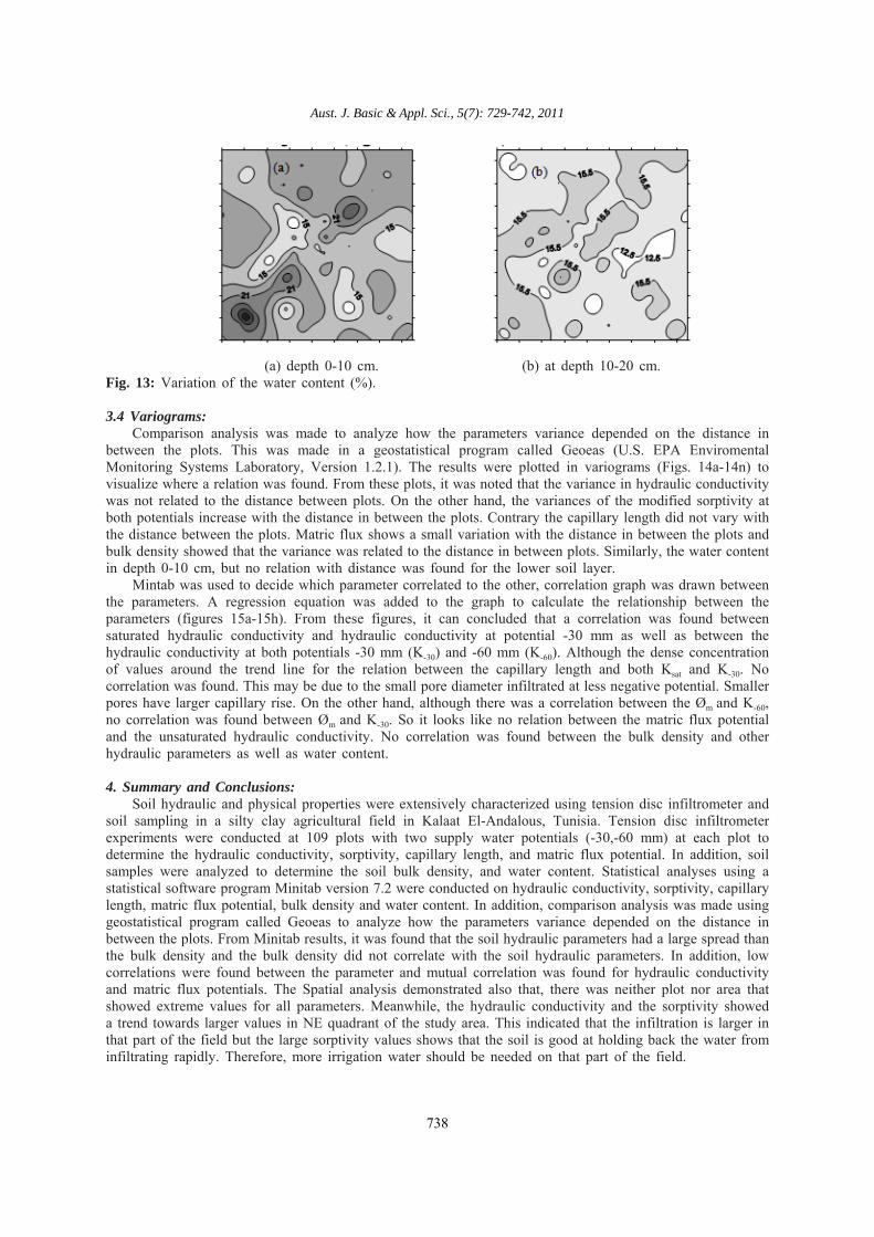
(a) depth 0-10 cm. (b) at depth 10-20 cm.Fig. 13: Variation of the water content (%).

3.4 Variograms:Comparison analysis was made to analyze how the parameters variance depended on the distance in

between the plots. This was made in a geostatistical program called Geoeas (U.S. EPA EnviromentalMonitoring Systems Laboratory, Version 1.2.1). The results were plotted in variograms (Figs. 14a-14n) tovisualize where a relation was found. From these plots, it was noted that the variance in hydraulic conductivitywas not related to the distance between plots. On the other hand, the variances of the modified sorptivity atboth potentials increase with the distance in between the plots. Contrary the capillary length did not vary withthe distance between the plots. Matric flux shows a small variation with the distance in between the plots andbulk density showed that the variance was related to the distance in between plots. Similarly, the water contentin depth 0-10 cm, but no relation with distance was found for the lower soil layer.

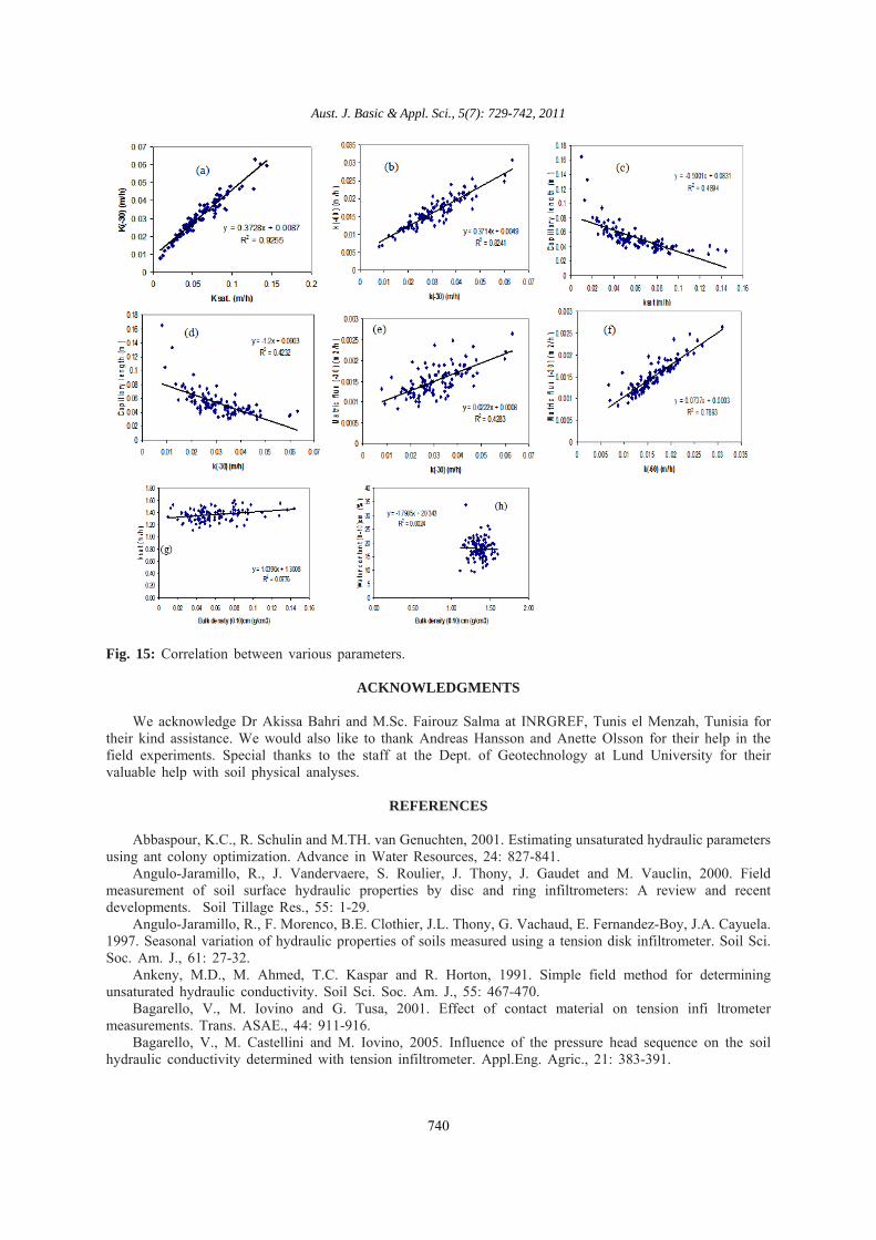
Mintab was used to decide which parameter correlated to the other, correlation graph was drawn betweenthe parameters. A regression equation was added to the graph to calculate the relationship between theparameters (figures 15a-15h). From these figures, it can concluded that a correlation was found betweensaturated hydraulic conductivity and hydraulic conductivity at potential -30 mm as well as between thehydraulic conductivity at both potentials -30 mm (K-30) and -60 mm (K-60). Although the dense concentrationof values around the trend line for the relation between the capillary length and both Ksat and K-30. Nocorrelation was found. This may be due to the small pore diameter infiltrated at less negative potential. Smallerpores have larger capillary rise. On the other hand, although there was a correlation between the Øm and K-60,no correlation was found between Øm and K-30. So it looks like no relation between the matric flux potentialand the unsaturated hydraulic conductivity. No correlation was found between the bulk density and otherhydraulic parameters as well as water content.

4. Summary and Conclusions:Soil hydraulic and physical properties were extensively characterized using tension disc infiltrometer and

soil sampling in a silty clay agricultural field in Kalaat El-Andalous, Tunisia. Tension disc infiltrometerexperiments were conducted at 109 plots with two supply water potentials (-30,-60 mm) at each plot todetermine the hydraulic conductivity, sorptivity, capillary length, and matric flux potential. In addition, soilsamples were analyzed to determine the soil bulk density, and water content. Statistical analyses using astatistical software program Minitab version 7.2 were conducted on hydraulic conductivity, sorptivity, capillarylength, matric flux potential, bulk density and water content. In addition, comparison analysis was made usinggeostatistical program called Geoeas to analyze how the parameters variance depended on the distance inbetween the plots. From Minitab results, it was found that the soil hydraulic parameters had a large spread thanthe bulk density and the bulk density did not correlate with the soil hydraulic parameters. In addition, lowcorrelations were found between the parameter and mutual correlation was found for hydraulic conductivityand matric flux potentials. The Spatial analysis demonstrated also that, there was neither plot nor area thatshowed extreme values for all parameters. Meanwhile, the hydraulic conductivity and the sorptivity showeda trend towards larger values in NE quadrant of the study area. This indicated that the infiltration is larger inthat part of the field but the large sorptivity values shows that the soil is good at holding back the water frominfiltrating rapidly. Therefore, more irrigation water should be needed on that part of the field.


739

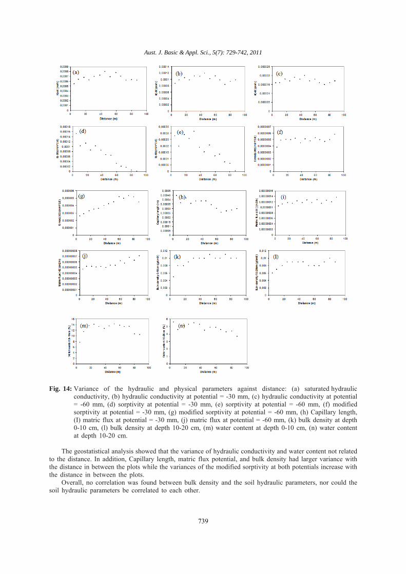
Fig. 14: Variance of the hydraulic and physical parameters against distance: (a) saturated hydraulicconductivity, (b) hydraulic conductivity at potential = -30 mm, (c) hydraulic conductivity at potential= -60 mm, (d) sorptivity at potential = -30 mm, (e) sorptivity at potential = -60 mm, (f) modifiedsorptivity at potential = -30 mm, (g) modified sorptivity at potential = -60 mm, (h) Capillary length,(I) matric flux at potential = -30 mm, (j) matric flux at potential = -60 mm, (k) bulk density at depth0-10 cm, (l) bulk density at depth 10-20 cm, (m) water content at depth 0-10 cm, (n) water contentat depth 10-20 cm.

The geostatistical analysis showed that the variance of hydraulic conductivity and water content not relatedto the distance. In addition, Capillary length, matric flux potential, and bulk density had larger variance withthe distance in between the plots while the variances of the modified sorptivity at both potentials increase withthe distance in between the plots.

Overall, no correlation was found between bulk density and the soil hydraulic parameters, nor could thesoil hydraulic parameters be correlated to each other.


740

Fig. 15: Correlation between various parameters.

ACKNOWLEDGMENTS

We acknowledge Dr Akissa Bahri and M.Sc. Fairouz Salma at INRGREF, Tunis el Menzah, Tunisia fortheir kind assistance. We would also like to thank Andreas Hansson and Anette Olsson for their help in thefield experiments. Special thanks to the staff at the Dept. of Geotechnology at Lund University for theirvaluable help with soil physical analyses.

REFERENCES

Abbaspour, K.C., R. Schulin and M.TH. van Genuchten, 2001. Estimating unsaturated hydraulic parametersusing ant colony optimization. Advance in Water Resources, 24: 827-841.

Angulo-Jaramillo, R., J. Vandervaere, S. Roulier, J. Thony, J. Gaudet and M. Vauclin, 2000. Fieldmeasurement of soil surface hydraulic properties by disc and ring infiltrometers: A review and recentdevelopments. Soil Tillage Res., 55: 1-29.

Angulo-Jaramillo, R., F. Morenco, B.E. Clothier, J.L. Thony, G. Vachaud, E. Fernandez-Boy, J.A. Cayuela.1997. Seasonal variation of hydraulic properties of soils measured using a tension disk infiltrometer. Soil Sci.Soc. Am. J., 61: 27-32.

Ankeny, M.D., M. Ahmed, T.C. Kaspar and R. Horton, 1991. Simple field method for determiningunsaturated hydraulic conductivity. Soil Sci. Soc. Am. J., 55: 467-470.

Bagarello, V., M. Iovino and G. Tusa, 2001. Effect of contact material on tension infi ltrometermeasurements. Trans. ASAE., 44: 911-916.

Bagarello, V., M. Castellini and M. Iovino, 2005. Influence of the pressure head sequence on the soilhydraulic conductivity determined with tension infiltrometer. Appl.Eng. Agric., 21: 383-391.


741

Baroni, G., A. Facchi, C. Gandolfi, B. Ortuani, D. Horeschi and J.C. van Dam, 2010. Uncertainty in thedetermination of soil hydraulic parameters and its influence on the performance of two hydrological modelsof different complexity. Hydrol. Earth Syst. Sci., 14: 251-270.

Close, K.R., G. Frasier, G.H. Dunn and J.C. Loftis, 1998. Tension infiltrometer contact interface evaluationby use of a potassium iodide tracer. Trans. ASAE, 41: 995-1004.

Clothier, B.E., M.B. Kirkham and J.E. McLean, 1992. In situ measurement of the effective transportvolume for solute moving through soil. Soil Sci. Soc. Am. J., 56: 733-736.

Gardner, W.R., 1958. Some steady state solutions to the unsaturated flow equation with application toevaporation from a water table. Soil Sci., 85: 228-232.

Hillel, D., 1971. Soil and Water. Academic press, New York.Hussen, A.A. and A.W. Warrick, 1993. Alternative analysis of hydraulic data from disc tension

infiltrometers. Water Resources Research, 29: 4103-4108. IRNAS and IAV, 2000. Progress report of the joint experiments between the IRNAS (Sevilla, Spain) and

IAV (Rabat, Morocco). Sixième rapport d’avancement Hydromed, ERBIC 18 CT 960091. HYDROMED.Johrar, R.K., J.C. van Dam, W.G.M. Bastiaansan and R.A. Feddes, 2004. Calibration of effective soil

hydraulic parameters of heterogeneoussoil profiles, J. Hydrol., 285: 233-247.Klute, A. (ed.), 1986. Methods of soil analysis. Part 1 –Physical and mineralogical methods. 2nd edition.

SSSJA book series: 5. Madison, Wisconsin, USA, pp: 791-796.Lamorski, K., Y. Pachepsky, C. Slawinski and R.T. Walczak, 2008. Using Support Vector Machines to

Develop Pedotransfer Functions for Water Retention of Soils in Poland. Soil Sci. Soc. Am. J., 72: 1243-1247.Logsdon, S.D. and D.B. Jaynes, 1993. Methodology for determining hydraulic conductivity with tension

infiltrometers. Soil Sci. Soc. Am. J., 57: 1426-1431.Messing, I. and N.J. Jarvis, 1993. Temporal variation in the hydraulic conductivity of a tilled clay soil as

measured by tension infiltrometers. Journal of Soil Science, 44: 11-24.Messing, I. and N.J. Jarvis, 1995. Near-saturated hydraulic conductivity in soils of contrasting texture

measured by tension infiltrometers. Soil Sci. Soc. Am. J., 59: 27-34.Minansy, B. and A.B. McBratney, 2002. The neuro-m method for fitting neural network parametric

pedotransfer functions. Soil Sci. Soc. Am. J., 66: 352-361.Nemes, A., M.G. Schaap and J.H.M. Wösten, 2003. Functional evaluation of pedotransfer functions derived

from different scales of data collection. Soil Sci. Soc. Am. J., 67: 1093-1102.Nemes, A., W.J. Rawls, Y.A. Pachepsky and M. Th.van Genuchten, 2006c. Sensitivity Analysis of the

Nonparametric Nearest Neighbor Technique to Estimate Soil Water Retention. Vadose Zone J., 5: 1222-1235.Perroux, K.M. and I. White, 1988. Design for disc permeameters. Soil Sci.Soc. Am. J., 52: 1205-1215.Philip, J.R., 1957. The theory of infiltration:4. Sorptivity and algebraic infiltration equations. Soil Sci., 84:

257-265.Quadri, M.B., B.E. Clothier, R. Angulo-Jaramillo, M. Vauclin and S.R. Green, 1994. Axisymmetric

transport of water and solute underneath a disk permeameter: Experiments and numerical model. Soil Sci. Soc.Am. J., 58: 696-703.

Reynolds, W.D. and D.E. Elrick, 1991. Determination of hydraulic conductivity using a tensioninfiltrometer. Soil Sci. Soc. Am. J., 55: 633-639.

Schaap, M.G., F.J. Leij and M. Th. van Genuchten, 2001. ROSETTA: A computer program for estimatingsoil hydraulic parameters with hierarchical pedotransfer functions. J. Hydrol., 251: 163-176.

Simunek, J. and M. Th. Van Genuchten, 1996. Estimating unsaturated soil hydraulic properties fromtension disc infiltrometer data by numerical inversion, Water Resour. Res., 32: 2683-2696.

Simunek, J., M. Th. Van Genuchten, M.M. Gribb and J.W. Hopmans, 1998. Parameter estimation ofunsaturated soil hydraulic properties from transient flow processes. Soil & Tillage Res., 47: 27-36.

Ungaro, F., C. Calzolari and E. Busoni, 2005. Development of pedotransfer functions using a groupmethod of data handling for the soil of the Pianura Padano–Veneta region of North Italy: water retentionproperties. Geoderma, 124: 293-317.

Vandervaere, J.P., M. Vauclin and D.E. Elrick, 2000. Transient flow from tension infiltrometers: I. Thetwo-parameter equation. Soil Sci. Soc. Am. J., 64: 1263-1272.

Villholt, K.G., K.H. Jensen and J. Fredericia, 1998. Flow and transport processes in a macroporoussubsurface-drained glacial till soil. J. Hydr., 207: 98-120.

White, I. and M.J. Sully, 1987. Macroscopic and microscopic capillary length and time scales from fieldinfiltration. Water Resour. Res., 23: 1514-1522.


742

Wooding, R.A., 1968. Steady infiltration from large shallow circular pond, Water Resour. Res., 4: 1259-1273.

Zhang, R., 1998. Estimating soil hydraulic conductivity and macroscopic capillary length from the diskinfiltrometer. Soil Sci. Soc. Am. J., 62: 1513-1521.

List of Notation:Ksat Saturated hydraulic conductivity, (LT-1).r Radius of circular source, (L).K0 Soil hydraulic conductivity corresponding to a given pressure head, (LT-1).S Sorptivity, (LT-0.5). K(ψ) Soil hydraulic conductivity at potential ψ, (LT-1).I Cumulative infiltration, (L).K(ψ1) Soil hydraulic conductivity at potential ψ1, (LT-1).t Cumulative time, (T).K(ψ2) Soil hydraulic conductivity at potential ψ2, (LT-1).λc Capillary length, (L).ψ, ψ1, ψ2 Potentials applied to the infiltrometer (L).Øm Matric flux potential, (L).α Contact angle (exponential slope), (L-1).

Documents

Spatial Analysis of Infiltration Experiment - ajbasweb.comajbasweb.com/old/ajbas/2011/July-2011/729-742.pdf · Australian Journal of Basic and Applied ... Spatial Analysis of Infiltration