Spatial Analysis and Modeling (GIST 4302/5302)

Guofeng Cao

Department of Geosciences

Texas Tech University

Outline

• Last week, we learned: – Review of map projection

– Characteristics of spatial data

– Types of spatial data

• This week, we will learn: – Concepts of database

– Representation of different types of spatial data in GIS

– Commonly used spatial operators in GIS

Database Fundaments

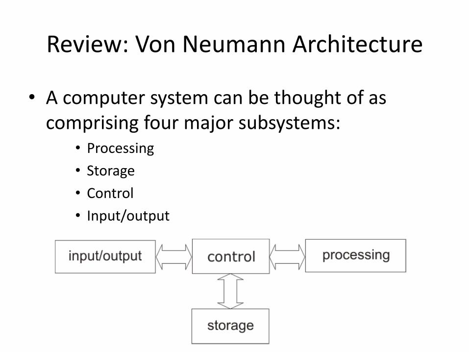
Review: Von Neumann Architecture

• A computer system can be thought of as comprising four major subsystems:

• Processing

• Storage

• Control

• Input/output

Review: Bits and Bytes

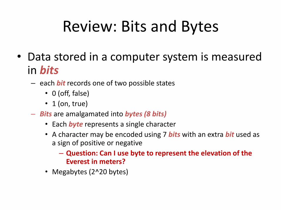
• Data stored in a computer system is measured in bits – each bit records one of two possible states

• 0 (off, false)

• 1 (on, true)

– Bits are amalgamated into bytes (8 bits)

• Each byte represents a single character

• A character may be encoded using 7 bits with an extra bit used as a sign of positive or negative

– Question: Can I use byte to represent the elevation of the Everest in meters?

• Megabytes (2^20 bytes)

Database

• A database is a collection of data organized in such a way that a computer can efficiently store and retrieve data

– A repository of data that is logically related

• A database is created and maintained using a general-purpose piece of software called a database management system (DBMS)

The Database Approach

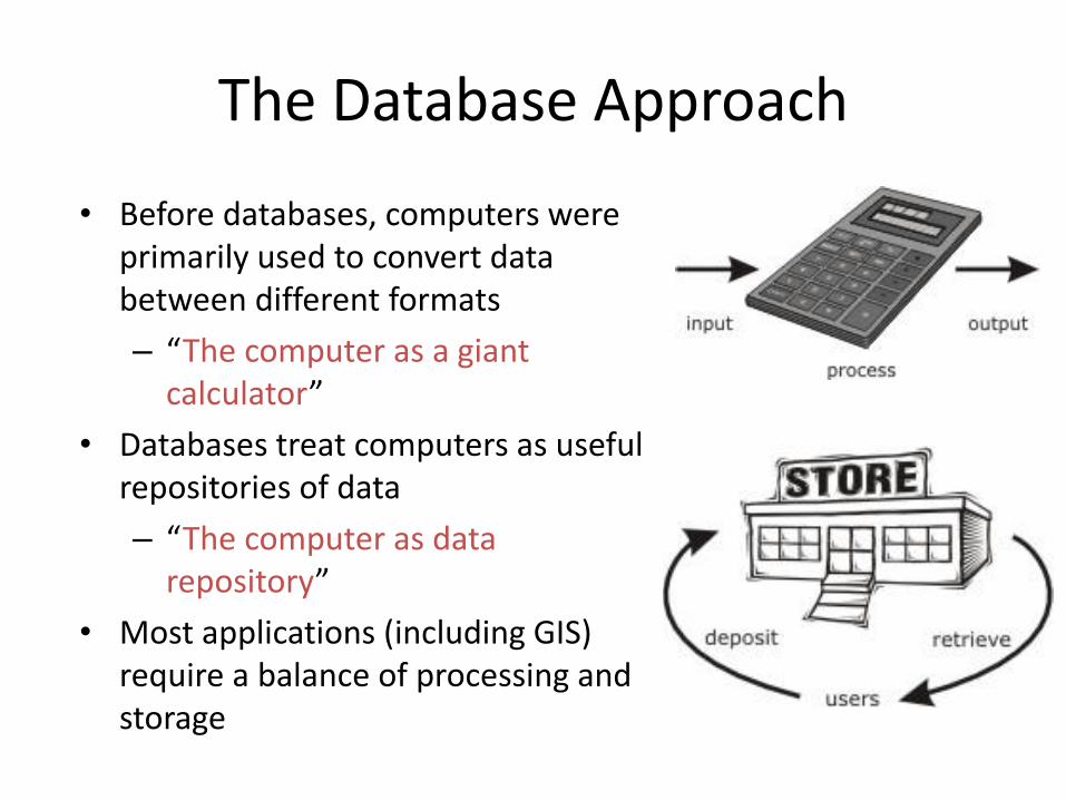
• Before databases, computers were primarily used to convert data between different formats

– “The computer as a giant calculator”

• Databases treat computers as useful repositories of data

– “The computer as data repository”

• Most applications (including GIS) require a balance of processing and storage

Databases in a Nutshell

• In order to be effective, databases must offer the following functions:

• All these functions are managed by the DBMS

– Reliability

– Integrity

– Security

– User views

– User interface

– Data independence

– Self-describing

– Concurrency

– Distributed capabilities

– High performance

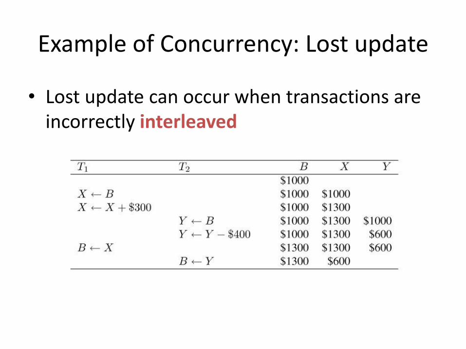
Example of Concurrency: Lost update

• Lost update can occur when transactions are incorrectly interleaved

Common Database Applications

• Home/office database – Simple applications (e.g., restaurant menus)

• Commercial database – Store the information for businesses (e.g. customers, employees)

• Engineering database – Used to store engineering designs (e.g. CAD)

• Image and multimedia database – Store image, audio, video data

• Geodatabase/spatial database – Store a combination of spatial and non-spatial data

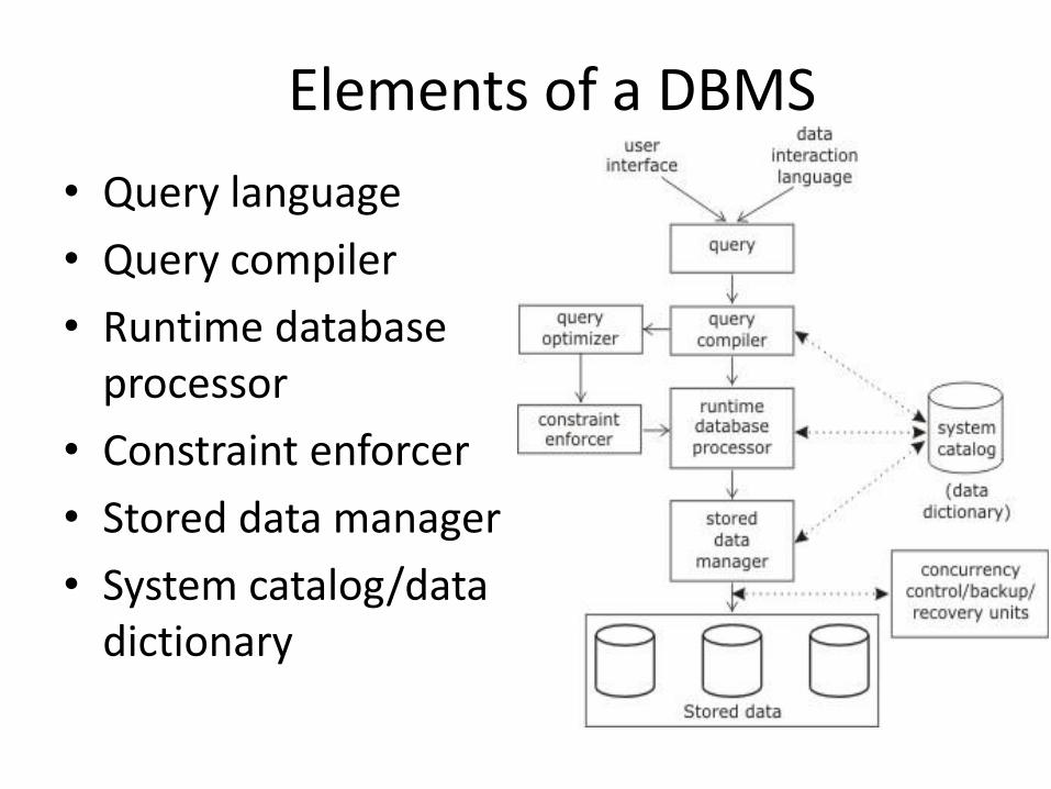
Elements of a DBMS

• Query language

• Query compiler

• Runtime database processor

• Constraint enforcer

• Stored data manager

• System catalog/data dictionary

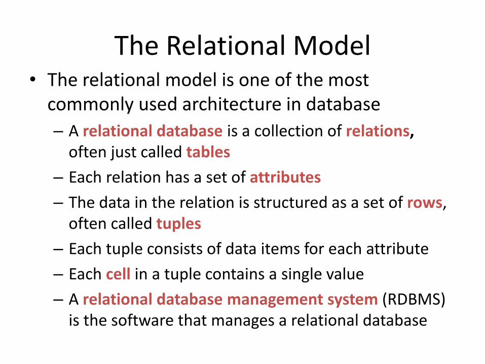
The Relational Model • The relational model is one of the most

commonly used architecture in database

– A relational database is a collection of relations, often just called tables

– Each relation has a set of attributes

– The data in the relation is structured as a set of rows, often called tuples

– Each tuple consists of data items for each attribute

– Each cell in a tuple contains a single value

– A relational database management system (RDBMS) is the software that manages a relational database

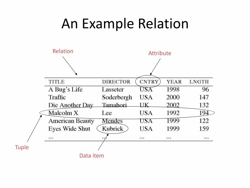
An Example Relation

Relation Attribute

Tuple

Data item

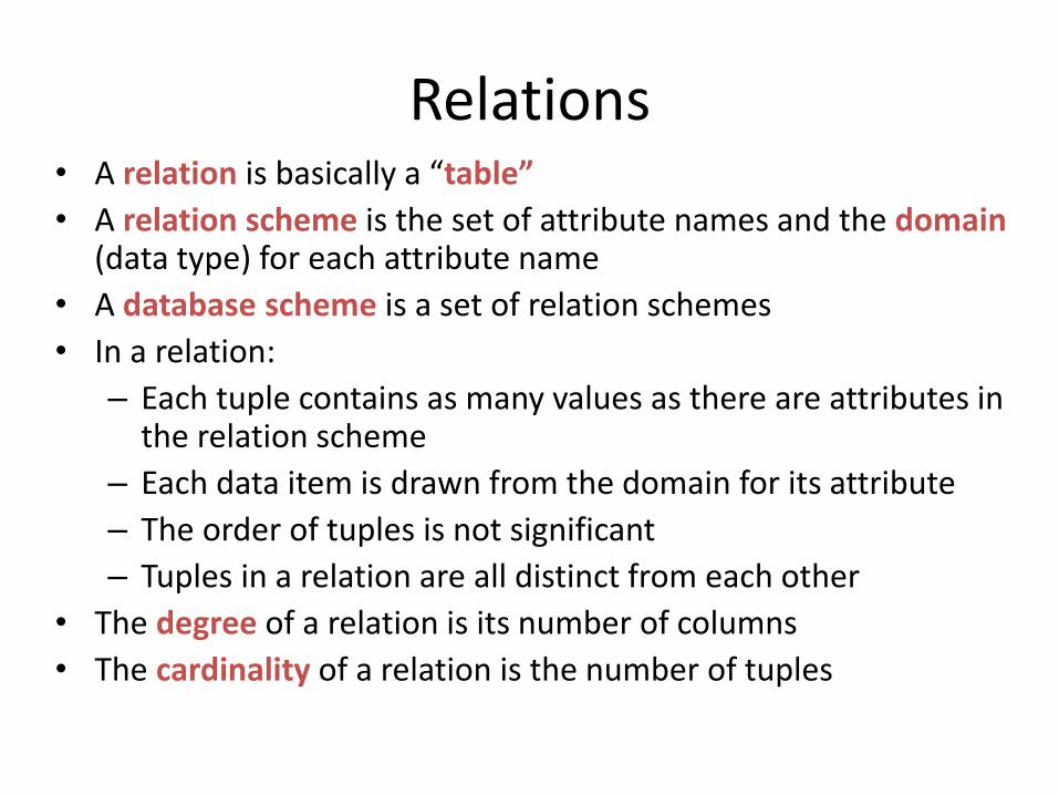
Relations • A relation is basically a “table”

• A relation scheme is the set of attribute names and the domain (data type) for each attribute name

• A database scheme is a set of relation schemes

• In a relation:

– Each tuple contains as many values as there are attributes in the relation scheme

– Each data item is drawn from the domain for its attribute

– The order of tuples is not significant

– Tuples in a relation are all distinct from each other

• The degree of a relation is its number of columns

• The cardinality of a relation is the number of tuples

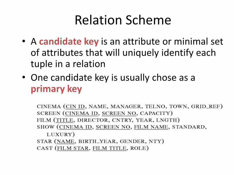
Relation Scheme

• A candidate key is an attribute or minimal set of attributes that will uniquely identify each tuple in a relation

• One candidate key is usually chose as a primary key

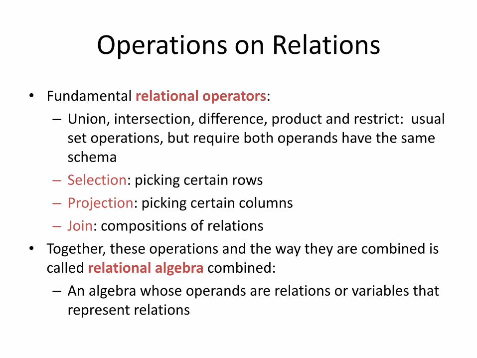
Operations on Relations

• Fundamental relational operators:

– Union, intersection, difference, product and restrict: usual set operations, but require both operands have the same schema

– Selection: picking certain rows

– Projection: picking certain columns

– Join: compositions of relations

• Together, these operations and the way they are combined is called relational algebra combined:

– An algebra whose operands are relations or variables that represent relations

Project Operator • The project operator is unary

– It outputs a new relation that has a subset of attributes

– Identical tuples in the output relation are coalesced

Relation Sells: bar beer price Chimy’s Bud 2.50 Chimy’s Miller 2.75 Cricket’s Bud 2.50 Cricket’s Miller 3.00

Prices := PROJbeer,price(Sells): beer price Bud 2.50 Miller 2.75 Miller 3.00

Select Operator

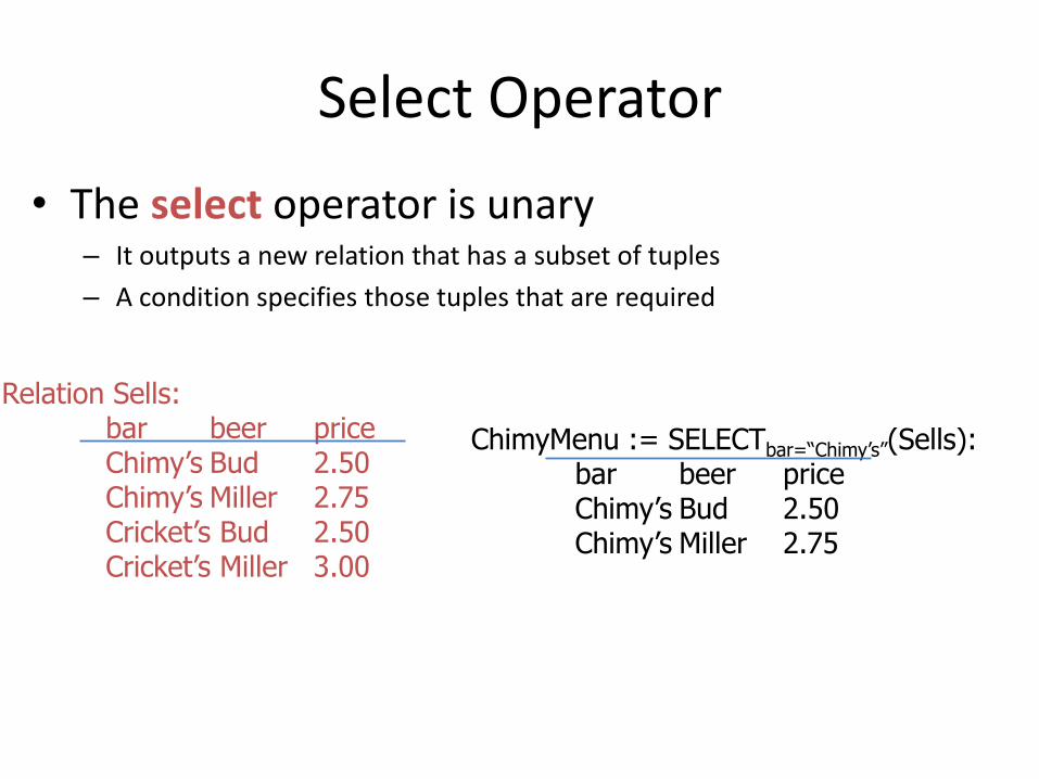
• The select operator is unary – It outputs a new relation that has a subset of tuples

– A condition specifies those tuples that are required

Relation Sells: bar beer price Chimy’s Bud 2.50 Chimy’s Miller 2.75 Cricket’s Bud 2.50 Cricket’s Miller 3.00

ChimyMenu := SELECTbar=“Chimy’s”(Sells): bar beer price Chimy’s Bud 2.50 Chimy’s Miller 2.75

Join Operator

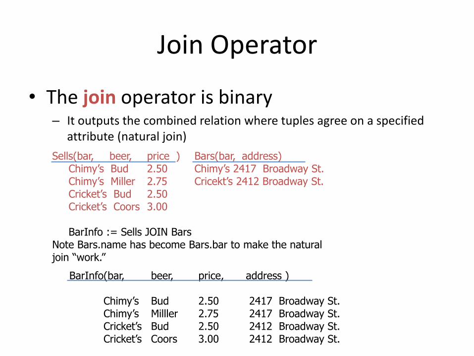
• The join operator is binary – It outputs the combined relation where tuples agree on a specified

attribute (natural join)

Sells(bar, beer, price ) Bars(bar, address) Chimy’s Bud 2.50 Chimy’s 2417 Broadway St. Chimy’s Miller 2.75 Cricekt’s 2412 Broadway St. Cricket’s Bud 2.50 Cricket’s Coors 3.00 BarInfo := Sells JOIN Bars Note Bars.name has become Bars.bar to make the natural join “work.”

BarInfo(bar, beer, price, address ) Chimy’s Bud 2.50 2417 Broadway St. Chimy’s Milller 2.75 2417 Broadway St. Cricket’s Bud 2.50 2412 Broadway St. Cricket’s Coors 3.00 2412 Broadway St.

Join Operator

• Join is the most time-consuming of all relational operators to compute – In general, relational operators may not be arbitrarily

reordered (left join, right join)

– Query optimization aims to find an efficient way of processing queries, for example reordering to produce equivalent but more efficient queries

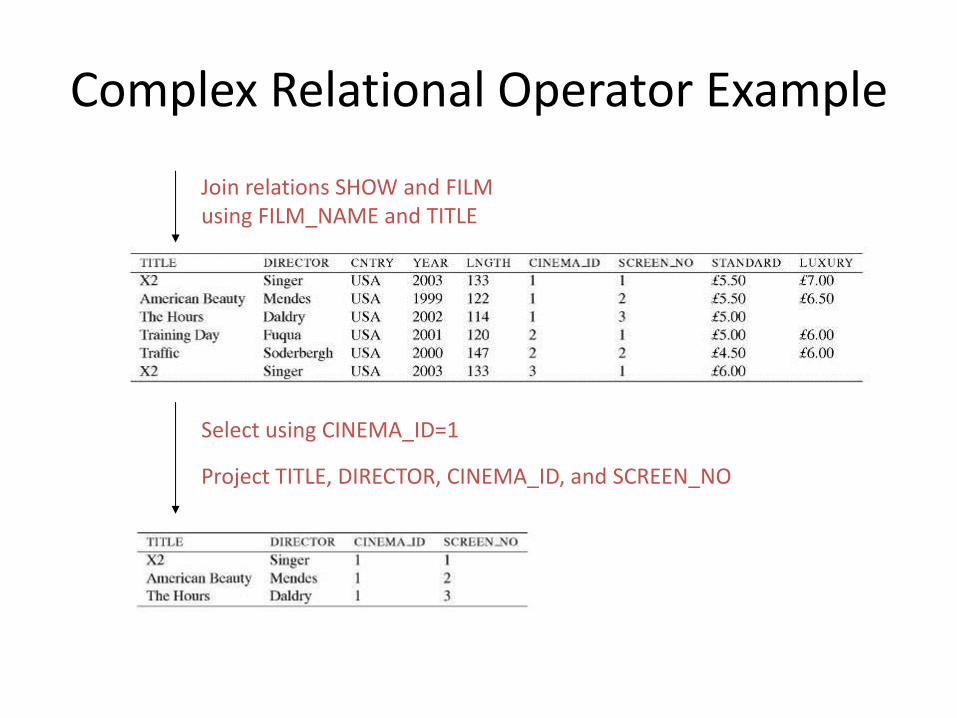
Complex Relational Operator Example

Join relations SHOW and FILM using FILM_NAME and TITLE

Select using CINEMA_ID=1

Project TITLE, DIRECTOR, CINEMA_ID, and SCREEN_NO

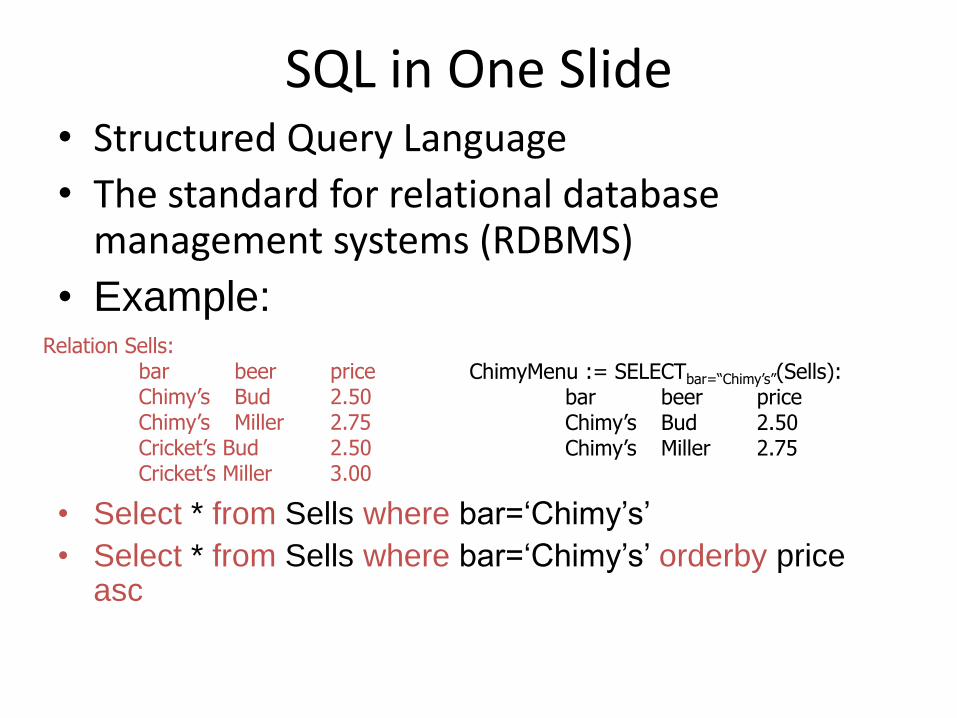
SQL in One Slide • Structured Query Language

• The standard for relational database management systems (RDBMS)

• Example:

• Select * from Sells where bar=‘Chimy’s’

• Select * from Sells where bar=‘Chimy’s’ orderby price asc

Relation Sells: bar beer price Chimy’s Bud 2.50 Chimy’s Miller 2.75 Cricket’s Bud 2.50 Cricket’s Miller 3.00

ChimyMenu := SELECTbar=“Chimy’s”(Sells): bar beer price Chimy’s Bud 2.50 Chimy’s Miller 2.75

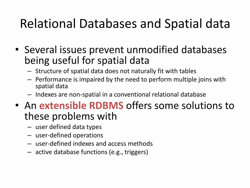
Relational Databases and Spatial data

• Several issues prevent unmodified databases being useful for spatial data – Structure of spatial data does not naturally fit with tables – Performance is impaired by the need to perform multiple joins with

spatial data – Indexes are non-spatial in a conventional relational database

• An extensible RDBMS offers some solutions to these problems with – user defined data types – user-defined operations – user-defined indexes and access methods – active database functions (e.g., triggers)

Representation of Spatial Data

Representation of Spatial Data Models

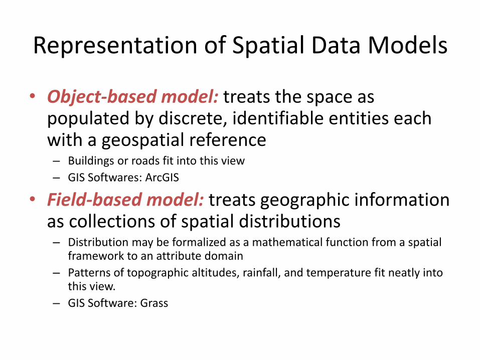
• Object-based model: treats the space as populated by discrete, identifiable entities each with a geospatial reference – Buildings or roads fit into this view

– GIS Softwares: ArcGIS

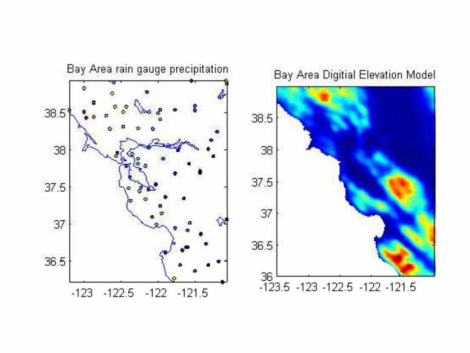
• Field-based model: treats geographic information as collections of spatial distributions – Distribution may be formalized as a mathematical function from a spatial

framework to an attribute domain

– Patterns of topographic altitudes, rainfall, and temperature fit neatly into this view.

– GIS Software: Grass

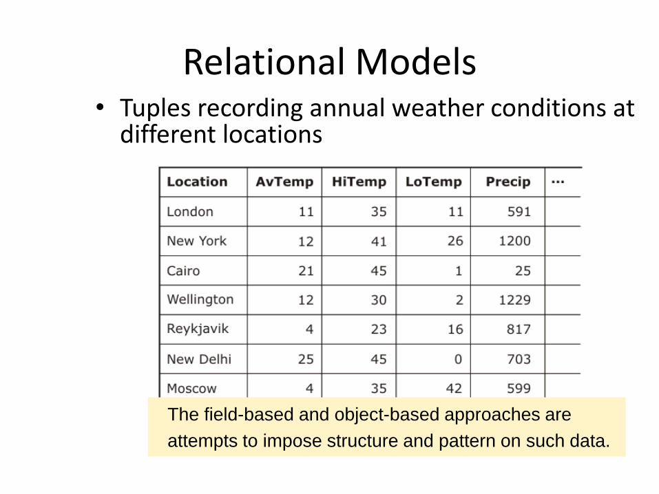
Relational Models • Tuples recording annual weather conditions at

different locations

The field-based and object-based approaches are

attempts to impose structure and pattern on such data.

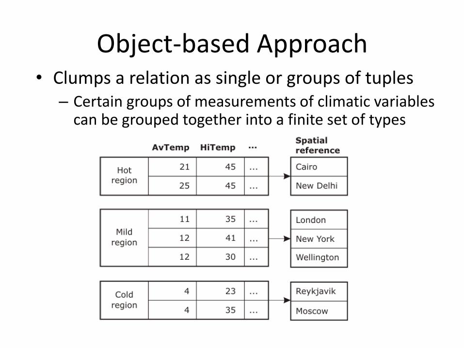
Object-based Approach • Clumps a relation as single or groups of tuples

– Certain groups of measurements of climatic variables can be grouped together into a finite set of types

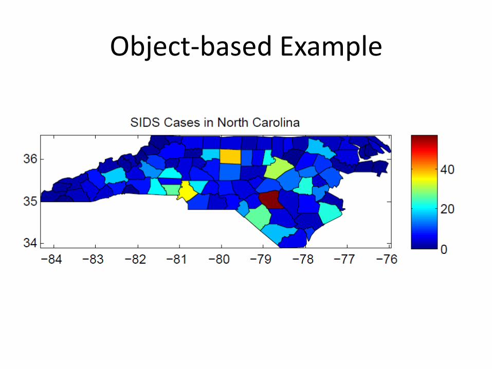
Object-based Example

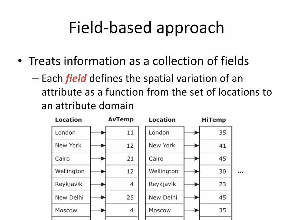
Field-based approach

• Treats information as a collection of fields

– Each field defines the spatial variation of an attribute as a function from the set of locations to an attribute domain

Object-based Approach

Entity

• Object-based models decompose an information space into objects or entities

• An entity must be: – Identifiable

– Relevant (be of interest)

– Describable (have characteristics)

• The frame of spatial reference is provided by the entities themselves

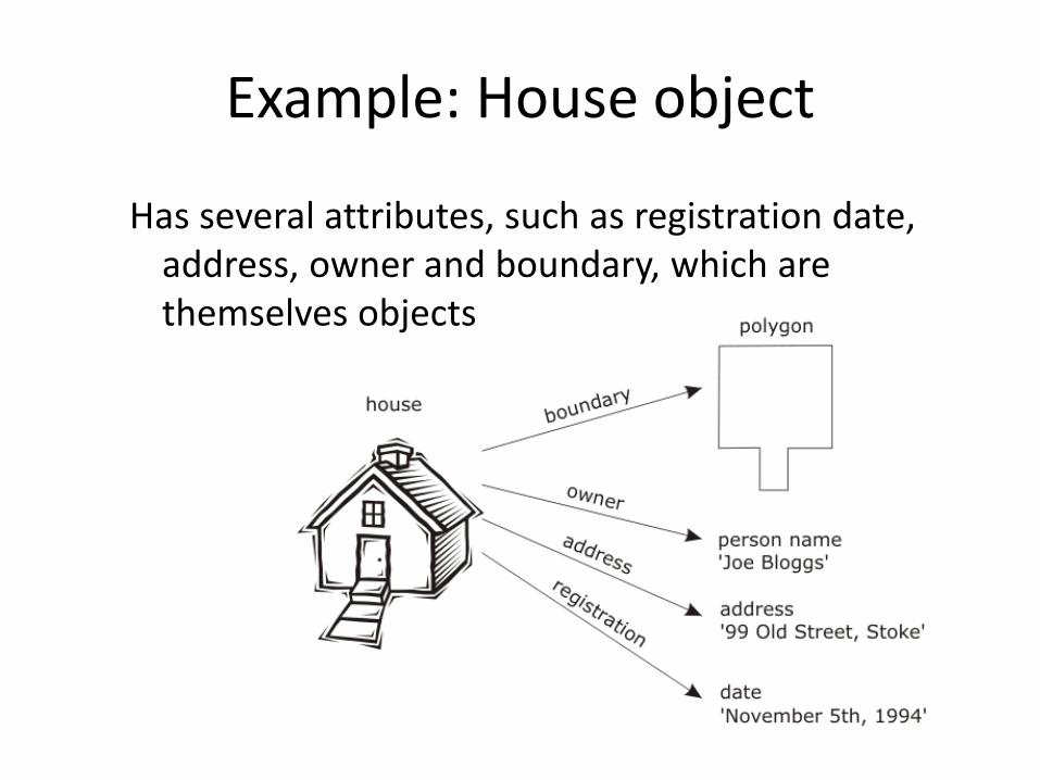
Example: House object

Has several attributes, such as registration date, address, owner and boundary, which are themselves objects

Spatial objects

• Spatial objects are called “spatial” because they exist inside “space”, called the embedding space

• A set of primitive objects can be specified, out of which all others in the application domain can be constructed, using an agreed set of operations

• Point-line-polygon primitives are common in existing systems

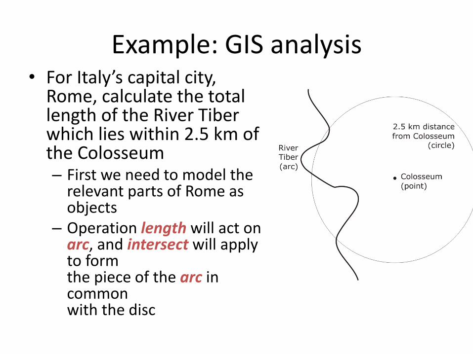
Example: GIS analysis • For Italy’s capital city,

Rome, calculate the total length of the River Tiber which lies within 2.5 km of the Colosseum – First we need to model the

relevant parts of Rome as objects

– Operation length will act on arc, and intersect will apply to form the piece of the arc in common with the disc

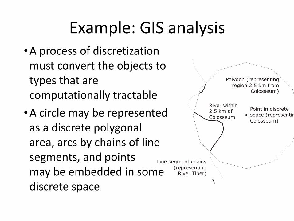
Example: GIS analysis •A process of discretization

must convert the objects to types that are computationally tractable

•A circle may be represented as a discrete polygonal area, arcs by chains of line segments, and points may be embedded in some discrete space

Primitive Objects

• Euclidean Space: coordinatized model of space

– Transforms spatial properties into properties of tuples of real numbers

– Coordinate frame consists of a fixed, distinguished point (origin) and a pair of orthogonal lines (axes), intersecting in the origin

• Point objects

• Line objects

• Polygonal objects

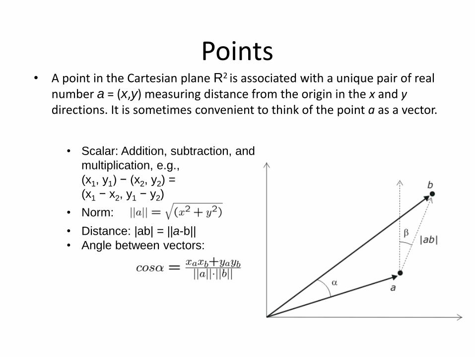
• Scalar: Addition, subtraction, and

multiplication, e.g.,

(x1, y1) − (x2, y2) =

(x1 − x2, y1 − y2)

• Norm:

• Distance: |ab| = ||a-b||

• Angle between vectors:

• A point in the Cartesian plane R2 is associated with a unique pair of real number a = (x,y) measuring distance from the origin in the x and y directions. It is sometimes convenient to think of the point a as a vector.

Points

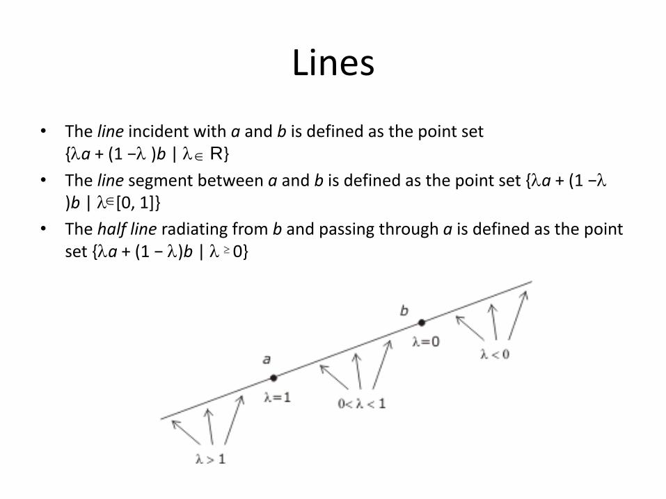
Lines

• The line incident with a and b is defined as the point set {a + (1 − )b | R}

• The line segment between a and b is defined as the point set {a + (1 − )b | [0, 1]}

• The half line radiating from b and passing through a is defined as the point set {a + (1 − )b | 0}

Polygonal objects

• A polyline in R2 is a finite set of line segments (called edges) such that each edge end-point is shared by exactly two edges, except possibly for two points, called the extremes of the polyline.

• If no two edges intersect at any place other than possibly at their end-points, the polyline is simple.

• A polyline is closed if it has no extreme points.

• A (simple) polygon in R2 is the area enclosed by a simple closed polyline. This polyline forms the boundary of the polygon. Each end-point of an edge of the polyline is called a vertex of the polygon.

• A convex polygon has every point intervisible

• A star-shaped or semi-convex polygon has at least one point that is intervisible

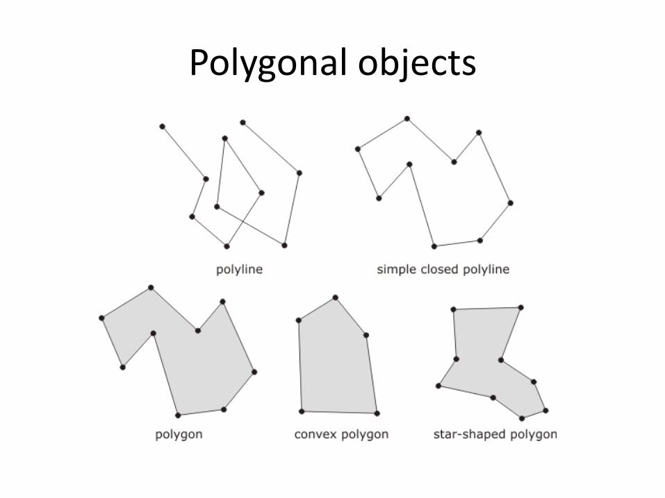
Polygonal objects

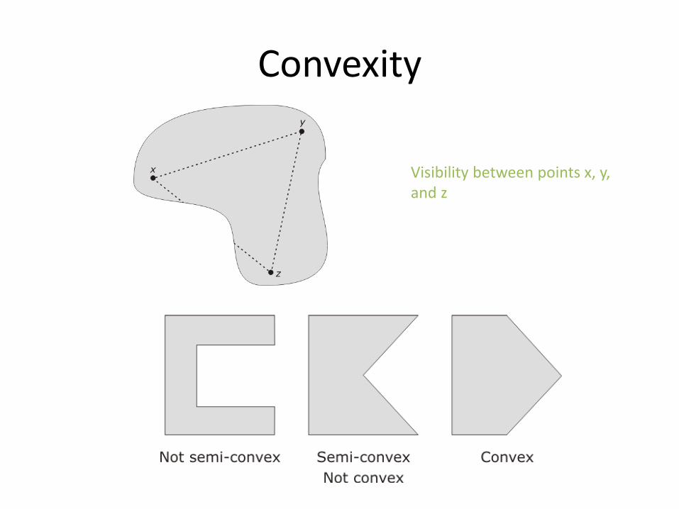
Convexity

Visibility between points x, y, and z

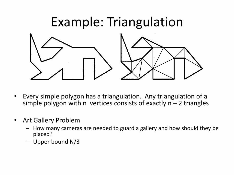
Example: Triangulation

• Every simple polygon has a triangulation. Any triangulation of a simple polygon with n vertices consists of exactly n – 2 triangles

• Art Gallery Problem – How many cameras are needed to guard a gallery and how should they be

placed?

– Upper bound N/3

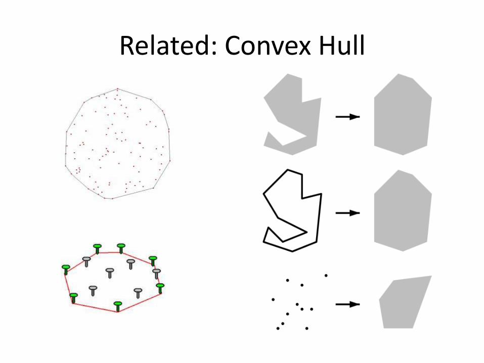
Related: Convex Hull

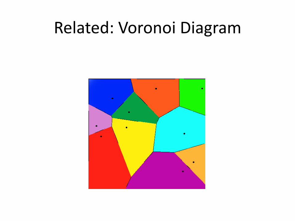
Related: Voronoi Diagram

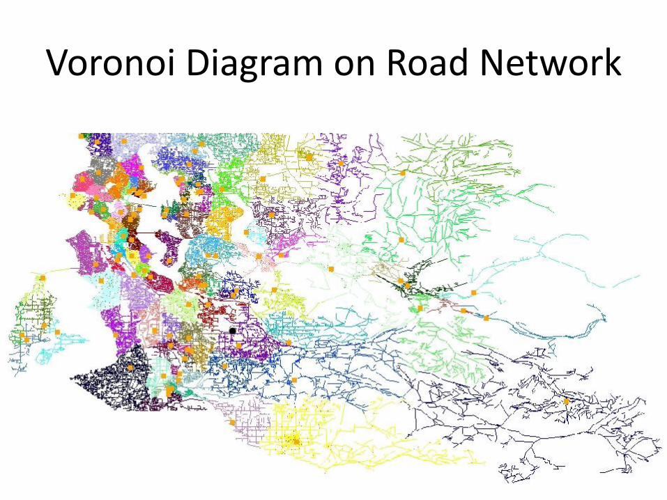
Voronoi Diagram on Road Network

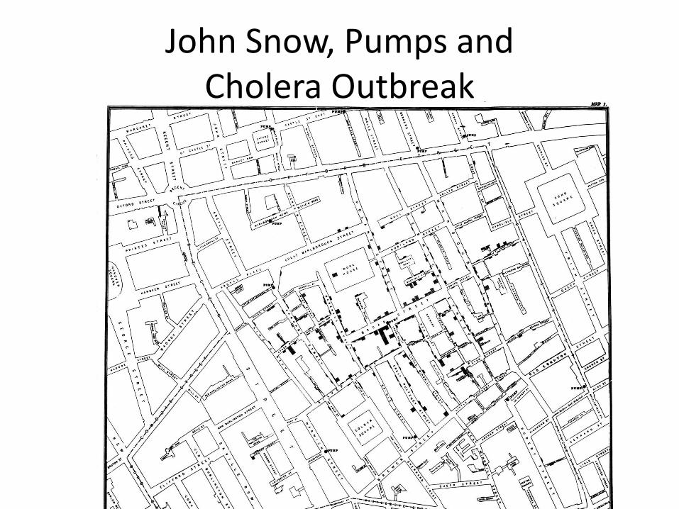
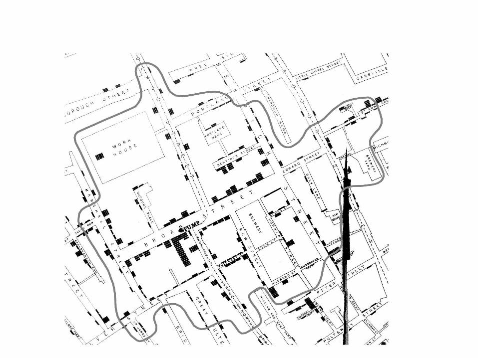
John Snow, Pumps and Cholera Outbreak

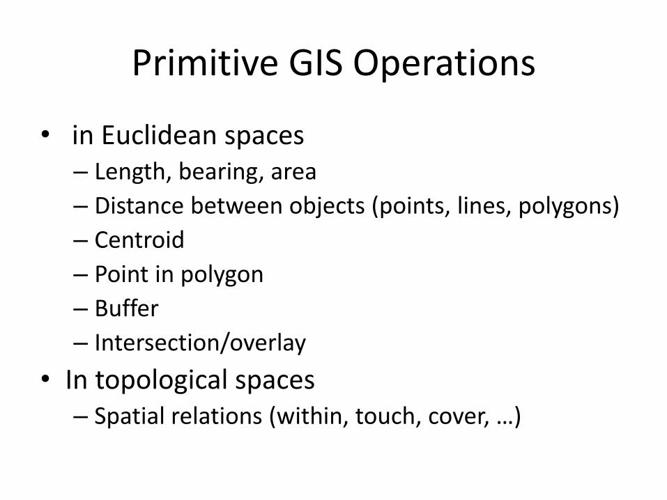
Primitive GIS Operations

• in Euclidean spaces – Length, bearing, area

– Distance between objects (points, lines, polygons)

– Centroid

– Point in polygon

– Buffer

– Intersection/overlay

• In topological spaces – Spatial relations (within, touch, cover, …)

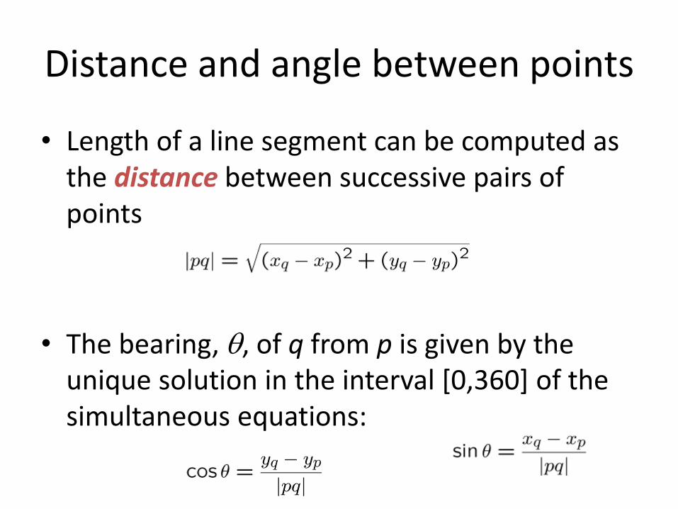
Distance and angle between points

• Length of a line segment can be computed as the distance between successive pairs of points

• The bearing, , of q from p is given by the unique solution in the interval [0,360] of the simultaneous equations:

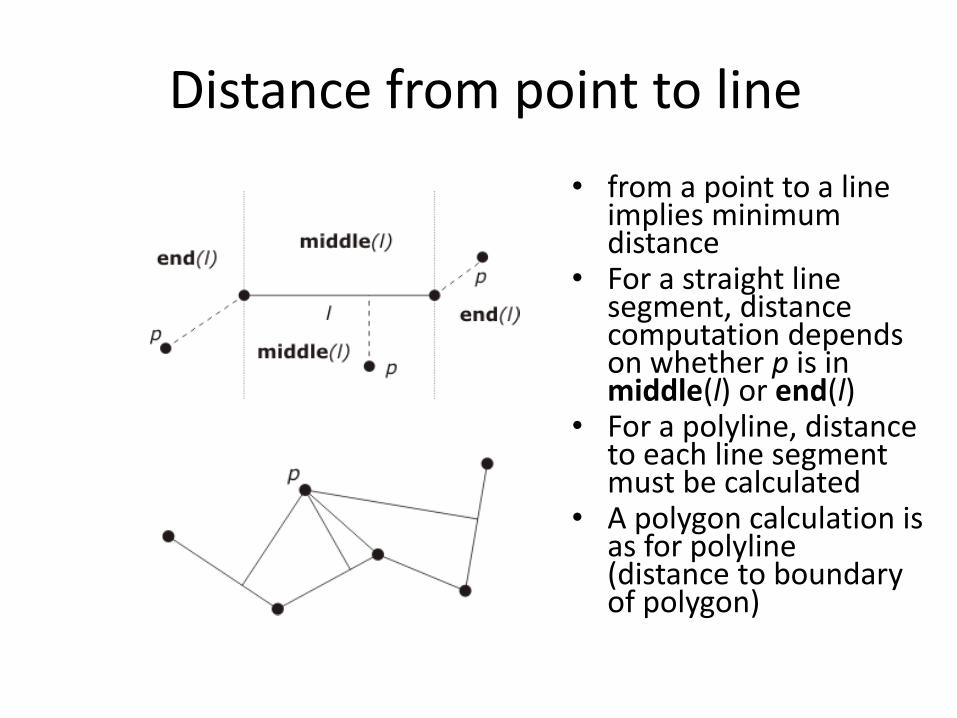
Distance from point to line

• from a point to a line implies minimum distance

• For a straight line segment, distance computation depends on whether p is in middle(l) or end(l)

• For a polyline, distance to each line segment must be calculated

• A polygon calculation is as for polyline (distance to boundary of polygon)

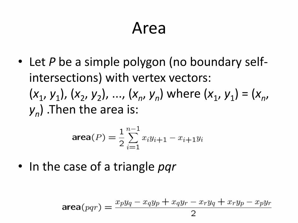
Area

• Let P be a simple polygon (no boundary self-intersections) with vertex vectors: (x1, y1), (x2, y2), ..., (xn, yn) where (x1, y1) = (xn, yn) .Then the area is:

• In the case of a triangle pqr

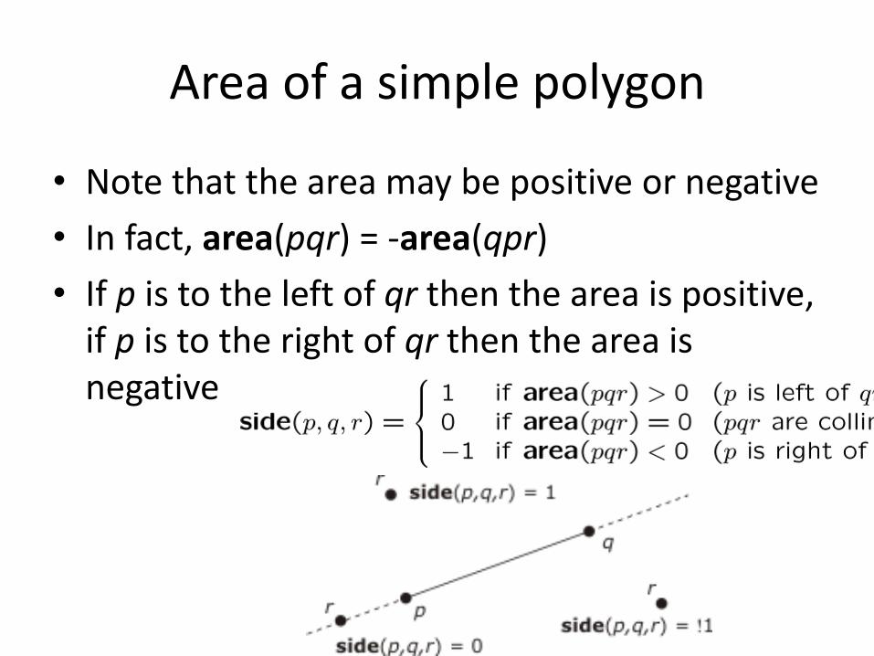
Area of a simple polygon

• Note that the area may be positive or negative

• In fact, area(pqr) = -area(qpr)

• If p is to the left of qr then the area is positive, if p is to the right of qr then the area is negative

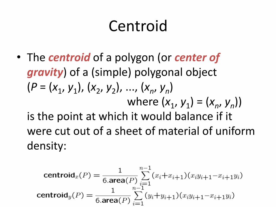
Centroid

• The centroid of a polygon (or center of gravity) of a (simple) polygonal object (P = (x1, y1), (x2, y2), ..., (xn, yn) where (x1, y1) = (xn, yn)) is the point at which it would balance if it were cut out of a sheet of material of uniform density:

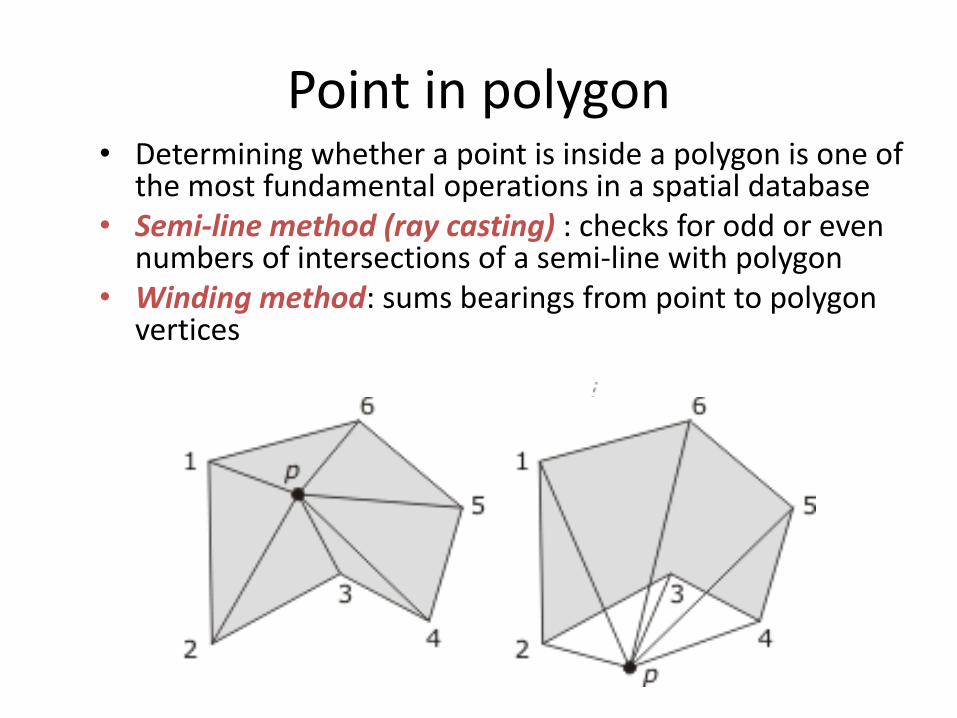
Point in polygon • Determining whether a point is inside a polygon is one of

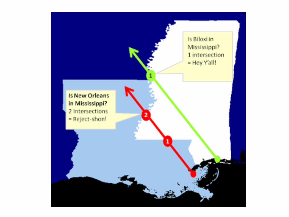
the most fundamental operations in a spatial database • Semi-line method (ray casting) : checks for odd or even

numbers of intersections of a semi-line with polygon • Winding method: sums bearings from point to polygon

vertices

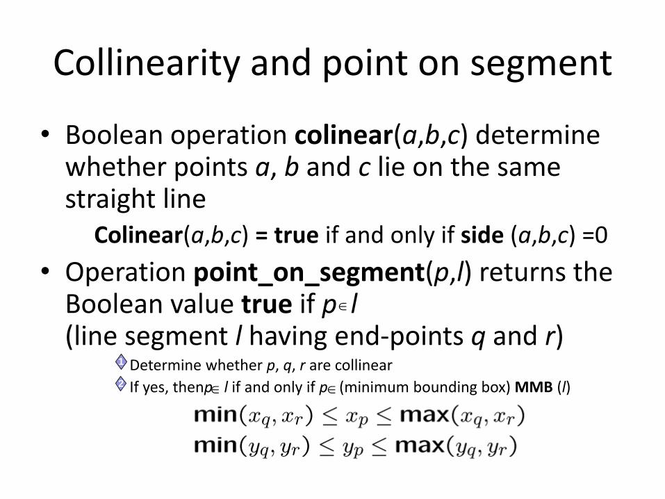
Collinearity and point on segment

• Boolean operation colinear(a,b,c) determine whether points a, b and c lie on the same straight line Colinear(a,b,c) = true if and only if side (a,b,c) =0

• Operation point_on_segment(p,l) returns the Boolean value true if p l (line segment l having end-points q and r)

11 Determine whether p, q, r are collinear 22 If yes, thenp l if and only if p (minimum bounding box) MMB (l)

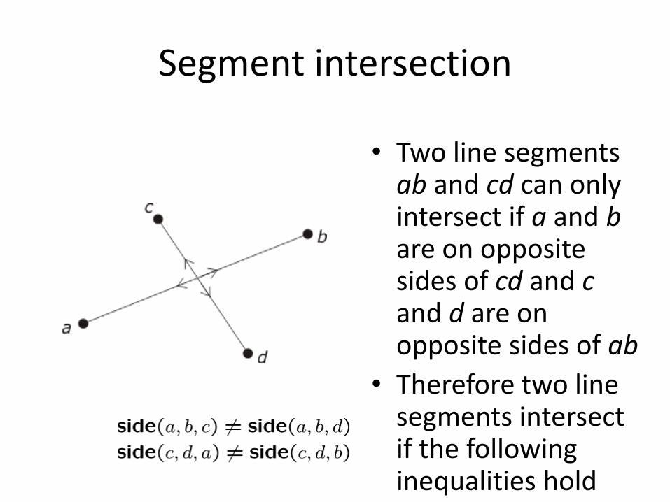
Segment intersection

• Two line segments ab and cd can only intersect if a and b are on opposite sides of cd and c and d are on opposite sides of ab

• Therefore two line segments intersect if the following inequalities hold

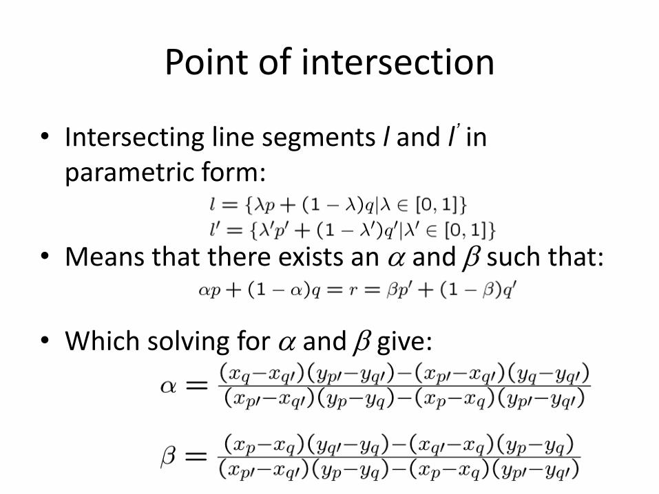
Point of intersection

• Intersecting line segments l and l’ in parametric form:

• Means that there exists an and such that:

• Which solving for and give:

Primitive GIS operations: Overlay

• Union

• Intersect

• Erase

• Identity

• Update

• Spatial Join

• Symmetrical Difference

Overlay

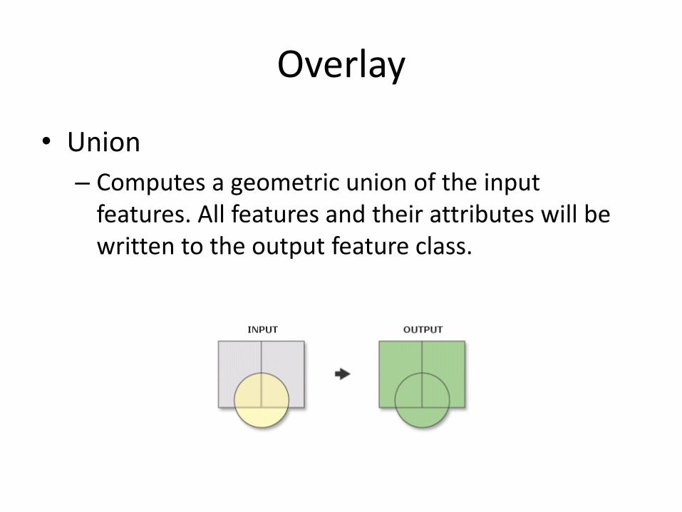
• Union

– Computes a geometric union of the input features. All features and their attributes will be written to the output feature class.

Overlay

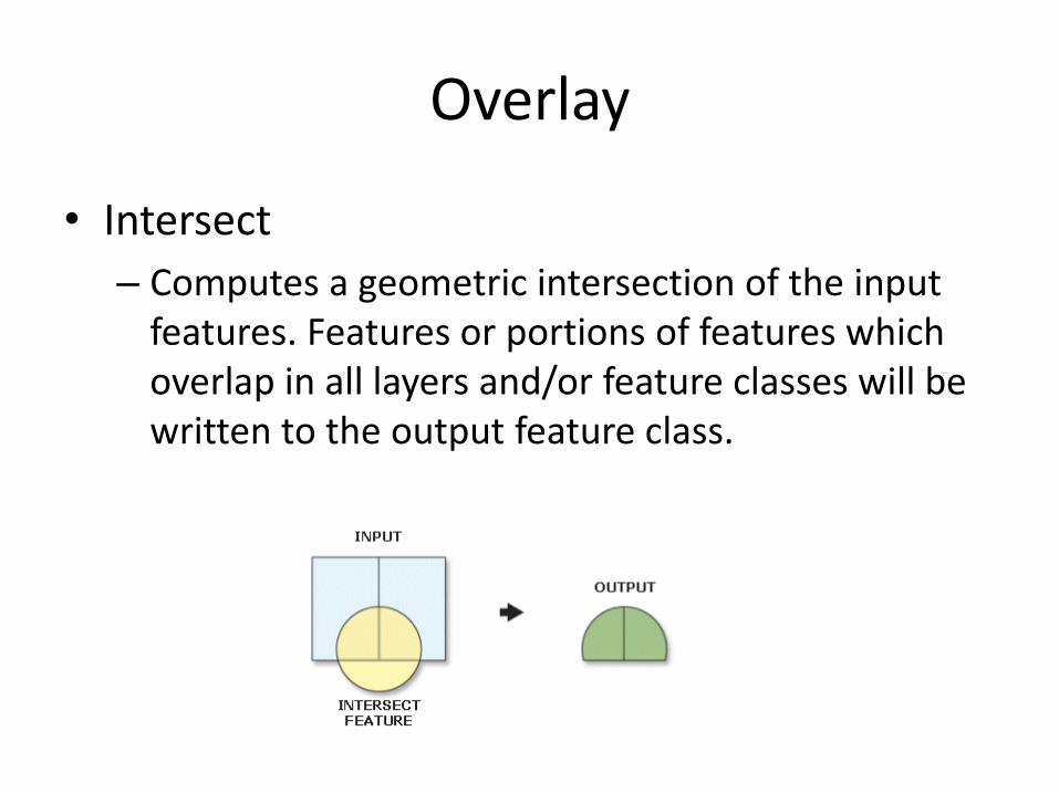
• Intersect

– Computes a geometric intersection of the input features. Features or portions of features which overlap in all layers and/or feature classes will be written to the output feature class.

Overlay

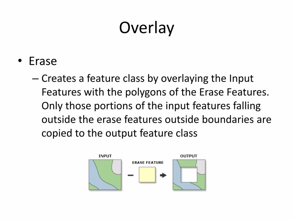
• Erase

– Creates a feature class by overlaying the Input Features with the polygons of the Erase Features. Only those portions of the input features falling outside the erase features outside boundaries are copied to the output feature class

Overlay

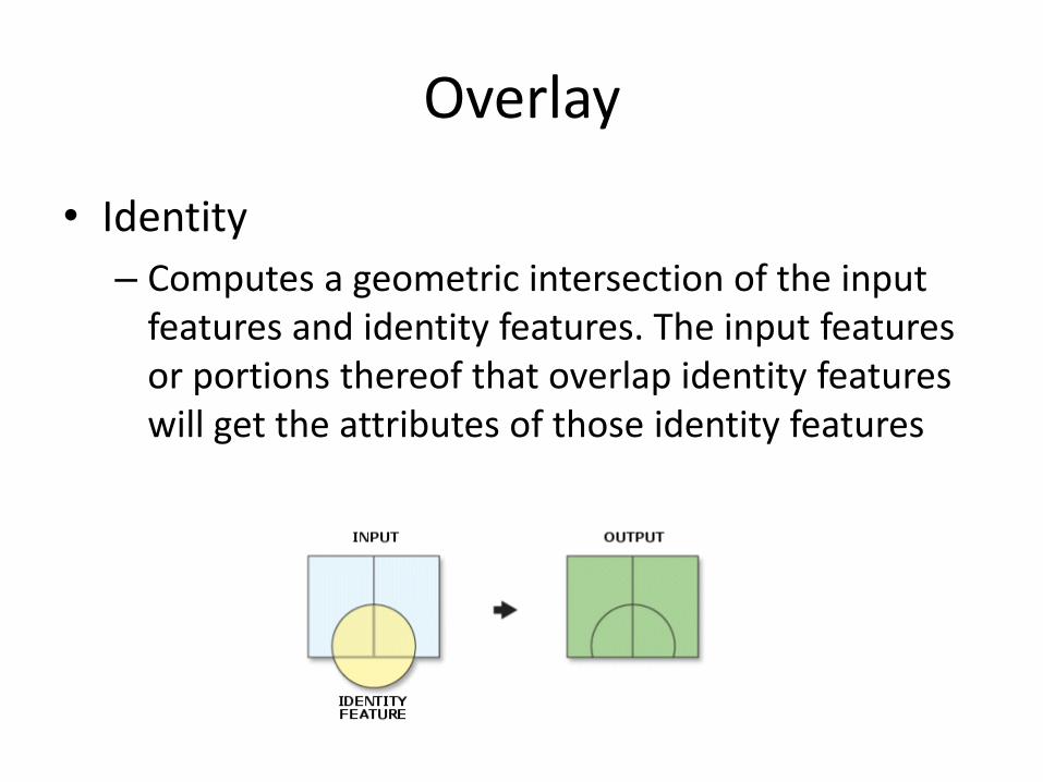
• Identity

– Computes a geometric intersection of the input features and identity features. The input features or portions thereof that overlap identity features will get the attributes of those identity features

Overlay

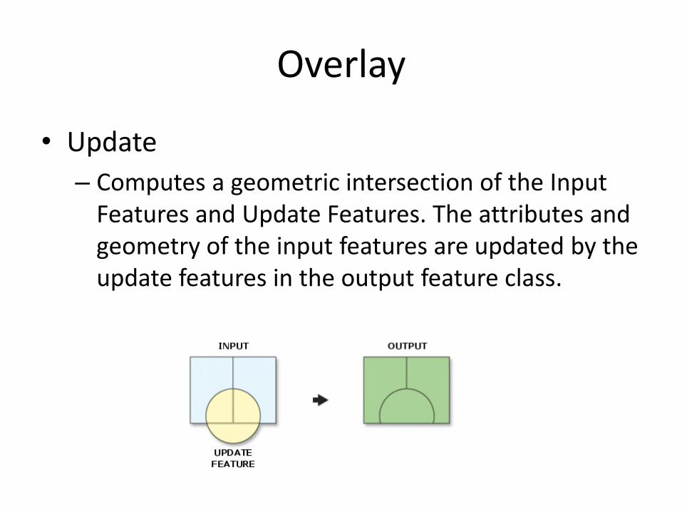
• Update

– Computes a geometric intersection of the Input Features and Update Features. The attributes and geometry of the input features are updated by the update features in the output feature class.

Overlay

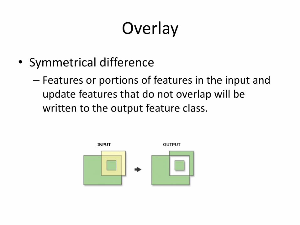
• Symmetrical difference

– Features or portions of features in the input and update features that do not overlap will be written to the output feature class.

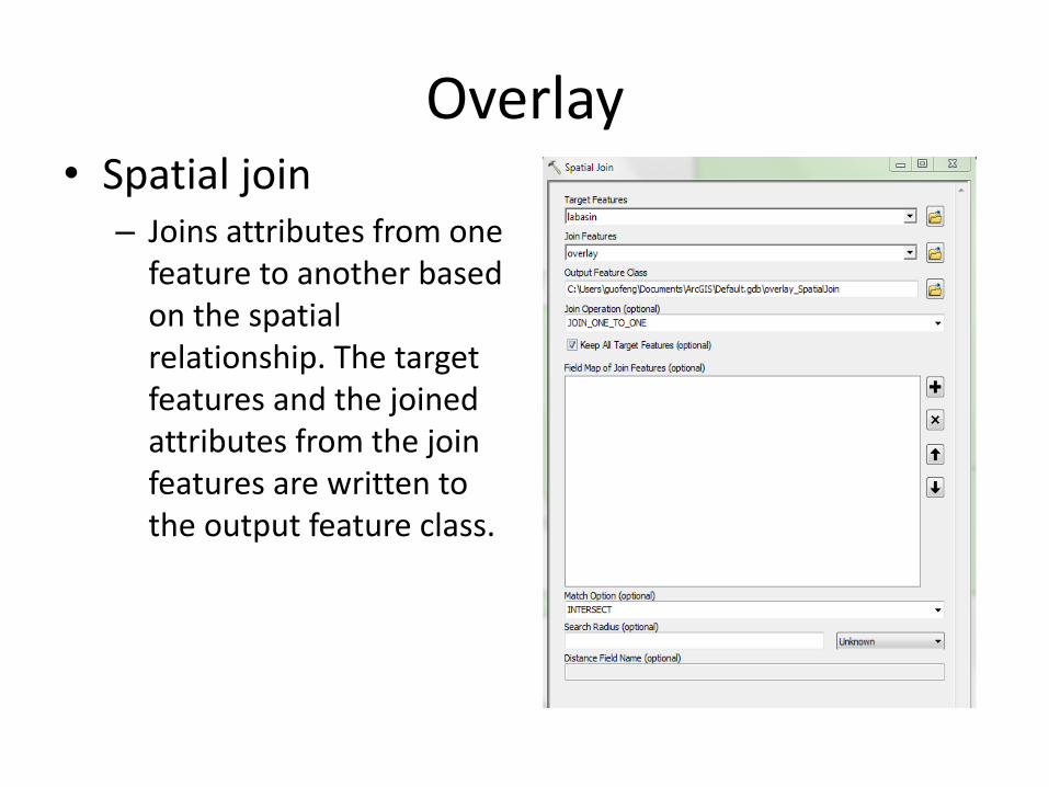
Overlay • Spatial join

– Joins attributes from one feature to another based on the spatial relationship. The target features and the joined attributes from the join features are written to the output feature class.

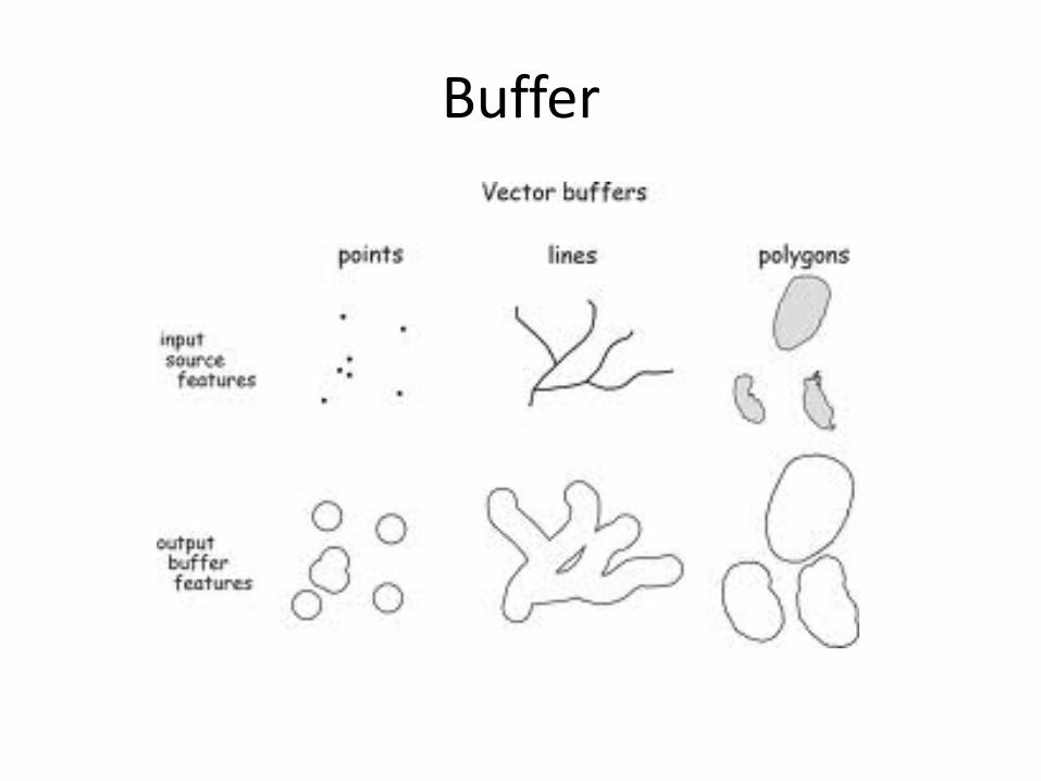
Buffer

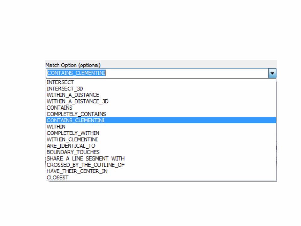
Topological spatial operations: spatial relationship

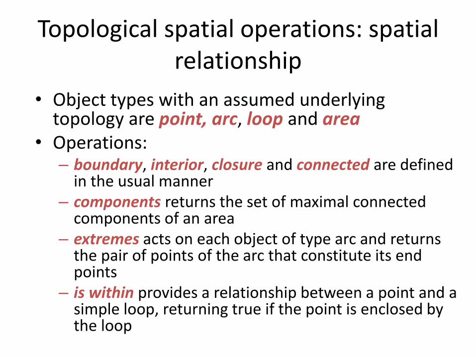
• Object types with an assumed underlying topology are point, arc, loop and area

• Operations: – boundary, interior, closure and connected are defined

in the usual manner – components returns the set of maximal connected

components of an area – extremes acts on each object of type arc and returns

the pair of points of the arc that constitute its end points

– is within provides a relationship between a point and a simple loop, returning true if the point is enclosed by the loop

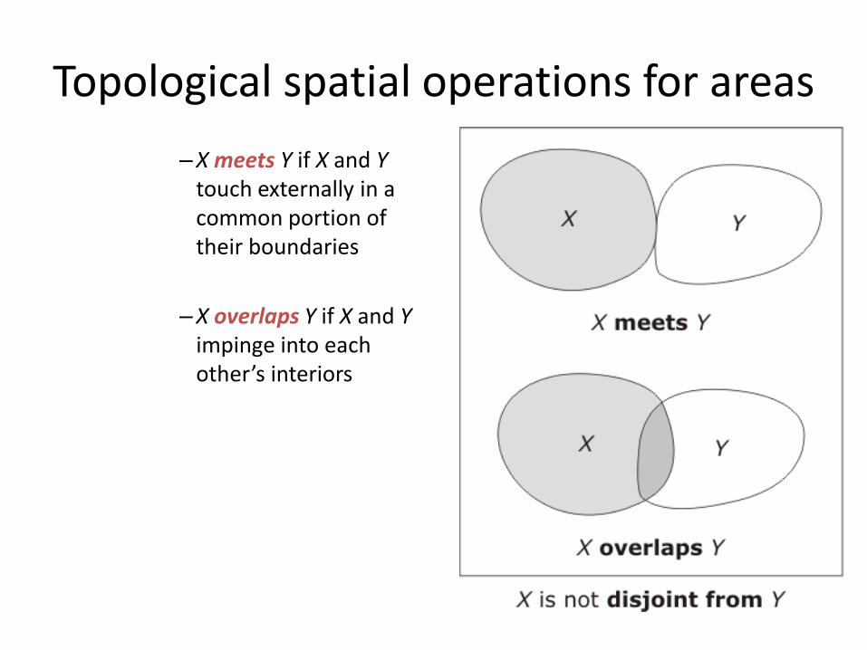
Topological spatial operations for areas

– X meets Y if X and Y touch externally in a common portion of their boundaries

– X overlaps Y if X and Y impinge into each other’s interiors

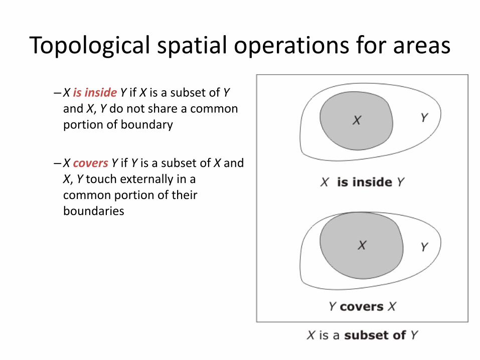
Topological spatial operations for areas

– X is inside Y if X is a subset of Y and X, Y do not share a common portion of boundary

– X covers Y if Y is a subset of X and X, Y touch externally in a common portion of their boundaries

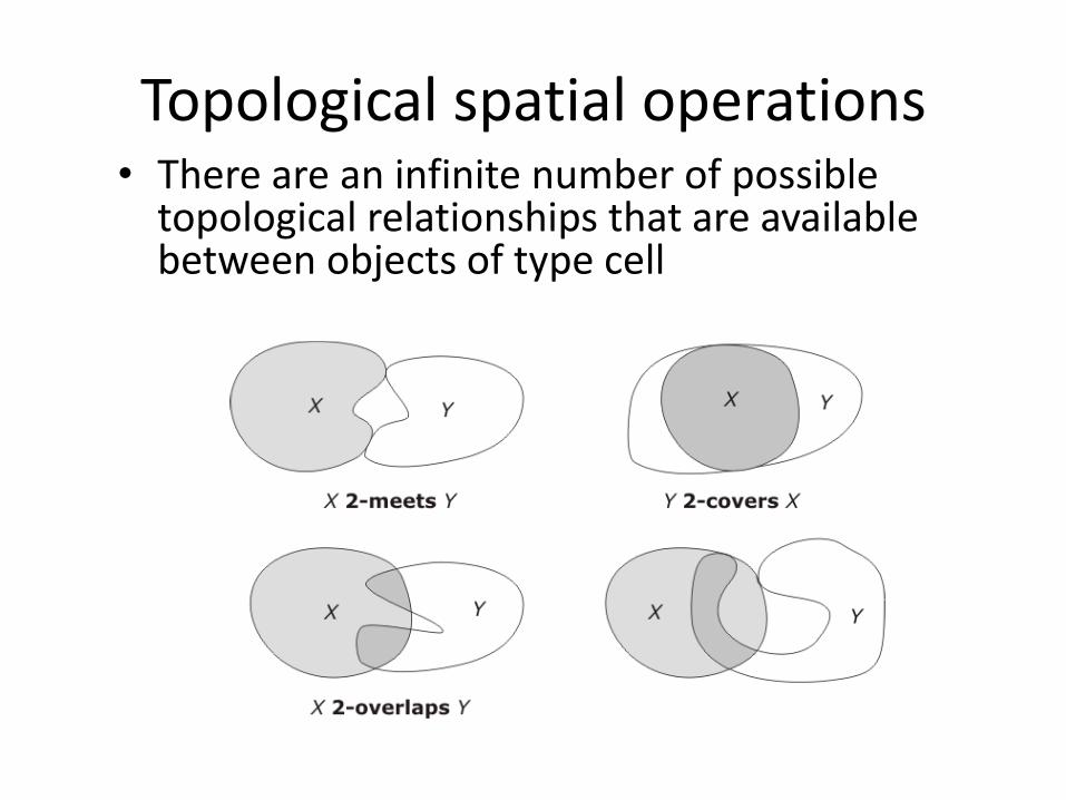
Topological spatial operations • There are an infinite number of possible

topological relationships that are available between objects of type cell

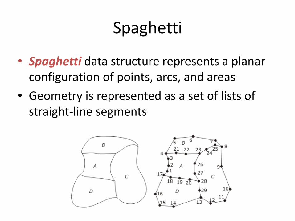
Spaghetti

• Spaghetti data structure represents a planar configuration of points, arcs, and areas

• Geometry is represented as a set of lists of straight-line segments

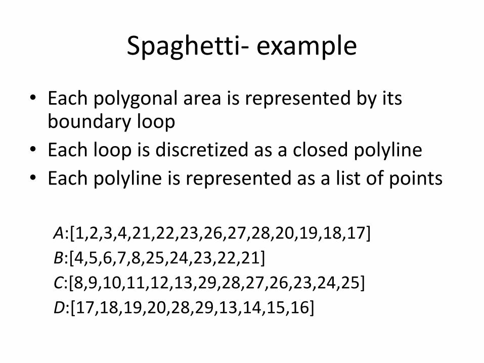
Spaghetti- example

• Each polygonal area is represented by its boundary loop

• Each loop is discretized as a closed polyline

• Each polyline is represented as a list of points

A:[1,2,3,4,21,22,23,26,27,28,20,19,18,17]

B:[4,5,6,7,8,25,24,23,22,21]

C:[8,9,10,11,12,13,29,28,27,26,23,24,25]

D:[17,18,19,20,28,29,13,14,15,16]

Issues

• There is NO explicit representation of the topological interrelationships of the configuration, such as adjacency

• Data consistence issues

– Silver polygons

– Data redundancy

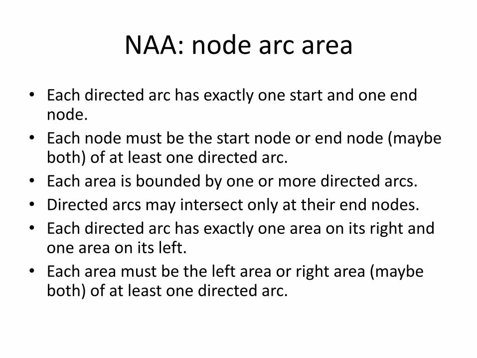
NAA: node arc area

• Each directed arc has exactly one start and one end node.

• Each node must be the start node or end node (maybe both) of at least one directed arc.

• Each area is bounded by one or more directed arcs.

• Directed arcs may intersect only at their end nodes.

• Each directed arc has exactly one area on its right and one area on its left.

• Each area must be the left area or right area (maybe both) of at least one directed arc.

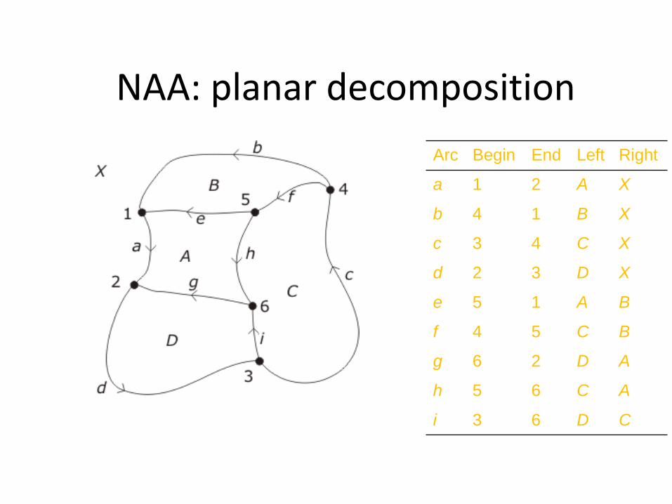
NAA: planar decomposition

Arc Begin End Left Right

a 1 2 A X

b 4 1 B X

c 3 4 C X

d 2 3 D X

e 5 1 A B

f 4 5 C B

g 6 2 D A

h 5 6 C A

i 3 6 D C

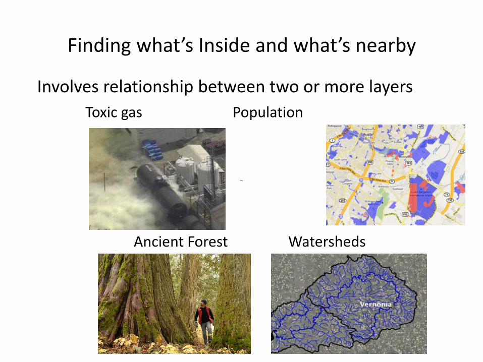
Finding what’s Inside and what’s nearby

Involves relationship between two or more layers

Toxic gas Population

Ancient Forest Watersheds

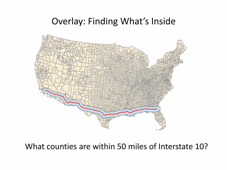
Overlay: Finding What’s Inside

What counties are within 50 miles of Interstate 10?

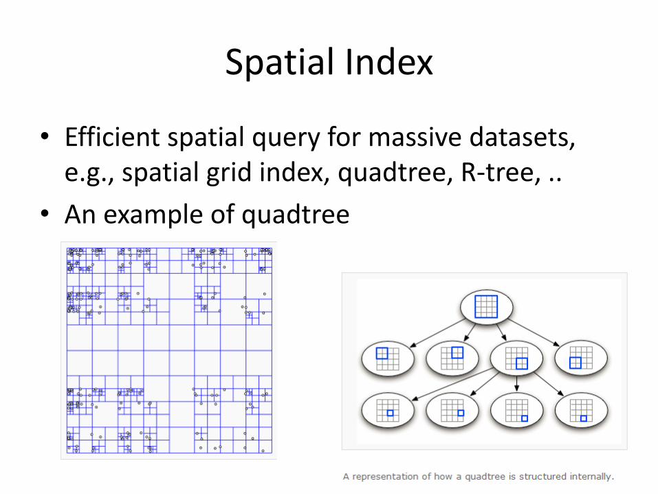
Spatial Index

• Efficient spatial query for massive datasets, e.g., spatial grid index, quadtree, R-tree, ..

• An example of quadtree

Field-based Approach

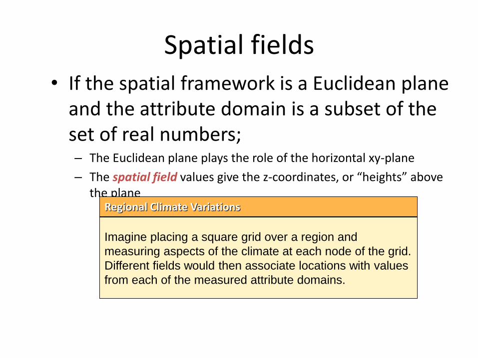
Spatial fields • If the spatial framework is a Euclidean plane

and the attribute domain is a subset of the set of real numbers; – The Euclidean plane plays the role of the horizontal xy-plane

– The spatial field values give the z-coordinates, or “heights” above the plane

Imagine placing a square grid over a region and

measuring aspects of the climate at each node of the grid.

Different fields would then associate locations with values

from each of the measured attribute domains.

Regional Climate Variations

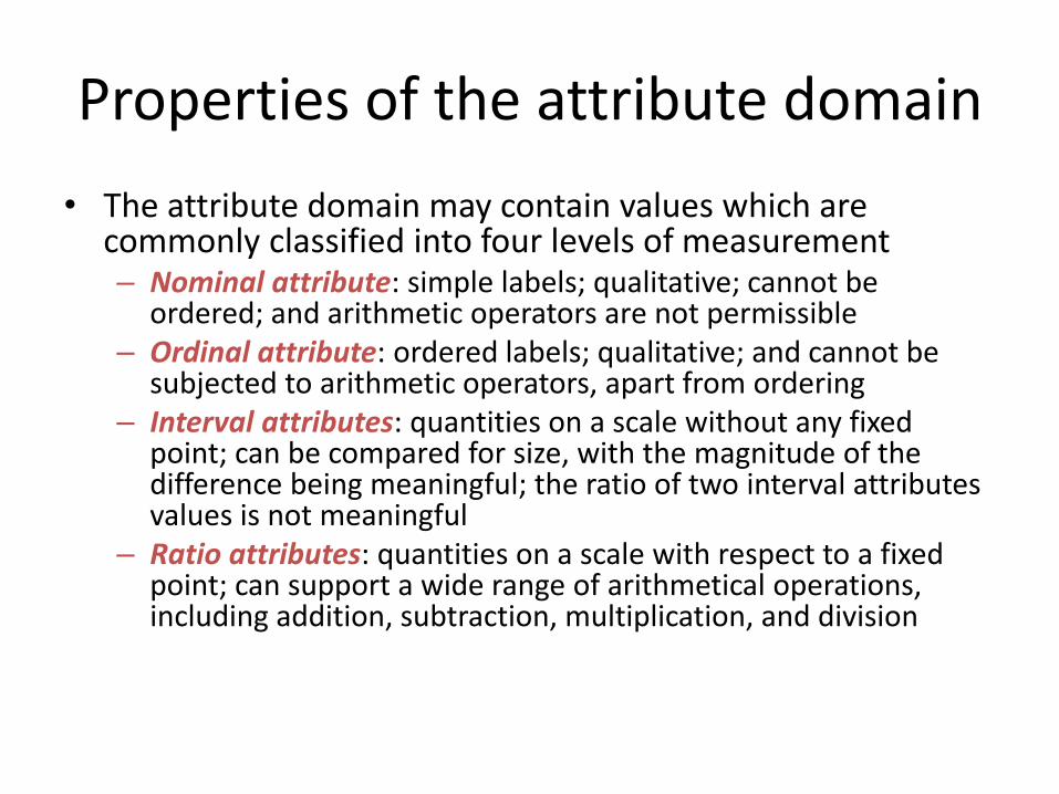
Properties of the attribute domain

• The attribute domain may contain values which are commonly classified into four levels of measurement – Nominal attribute: simple labels; qualitative; cannot be

ordered; and arithmetic operators are not permissible – Ordinal attribute: ordered labels; qualitative; and cannot be

subjected to arithmetic operators, apart from ordering – Interval attributes: quantities on a scale without any fixed

point; can be compared for size, with the magnitude of the difference being meaningful; the ratio of two interval attributes values is not meaningful

– Ratio attributes: quantities on a scale with respect to a fixed point; can support a wide range of arithmetical operations, including addition, subtraction, multiplication, and division

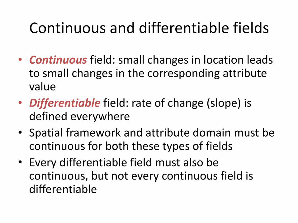
Continuous and differentiable fields

• Continuous field: small changes in location leads to small changes in the corresponding attribute value

• Differentiable field: rate of change (slope) is defined everywhere

• Spatial framework and attribute domain must be continuous for both these types of fields

• Every differentiable field must also be continuous, but not every continuous field is differentiable

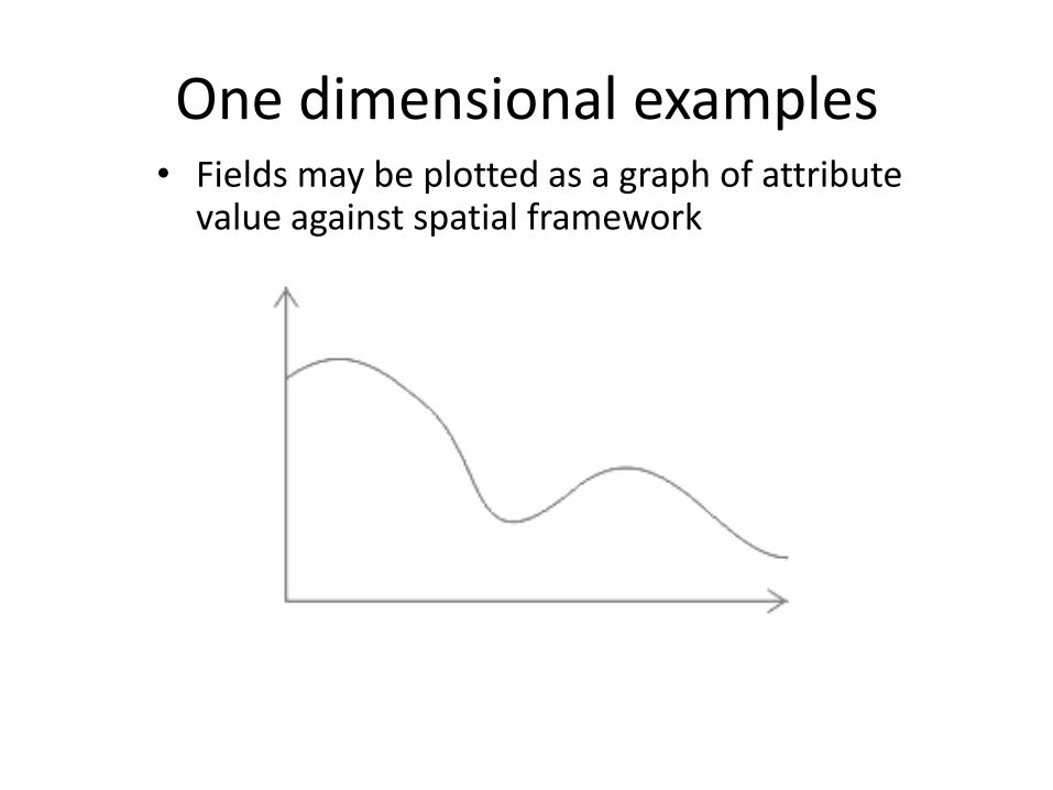
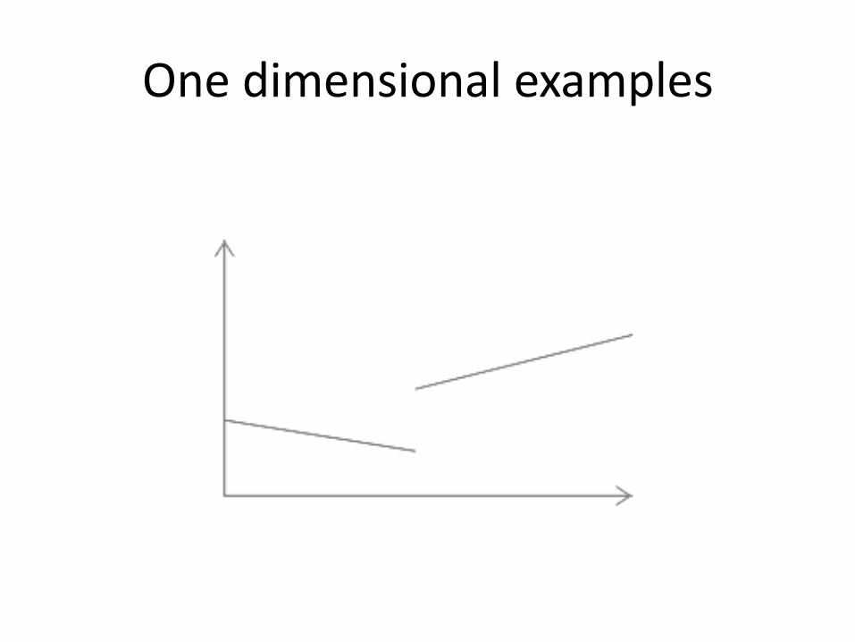
One dimensional examples • Fields may be plotted as a graph of attribute

value against spatial framework

Continuous and differentiable; the slope of the curve can be

defined at every point

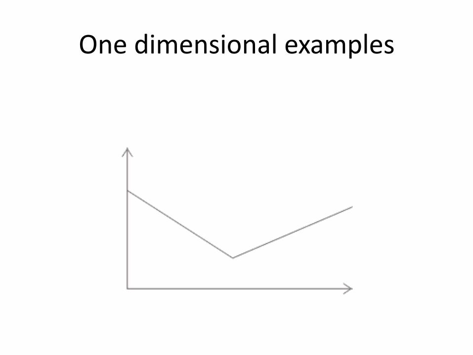
One dimensional examples The field is continuous (the graph is connected) but not

everywhere differentiable. There is an ambiguity in the slope,

with two choices at the articulation point between the two

straight line segments.

Continuous and not differentiable; the slope of the curve cannot

be defined at one or more points

One dimensional examples

The graph is not connected and so the field in not continuous

and not differentiable.

Not continuous and not differentiable

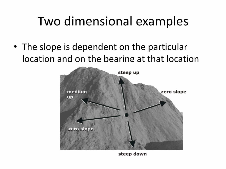
Two dimensional examples

• The slope is dependent on the particular location and on the bearing at that location

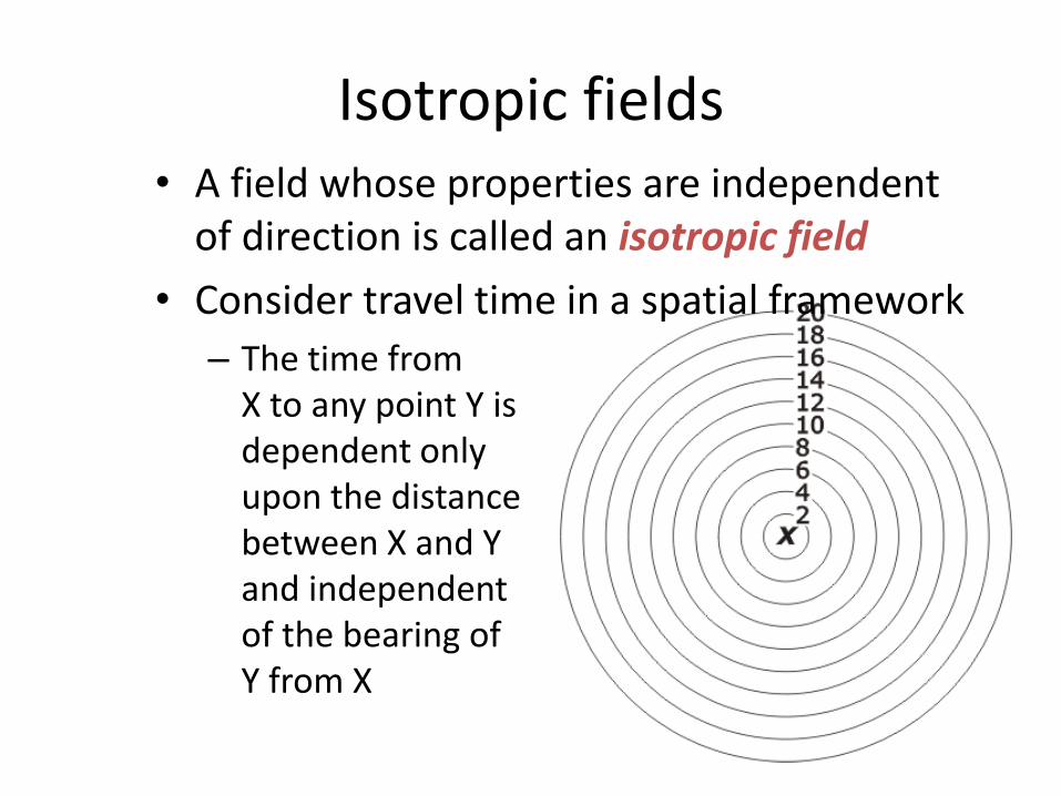
Isotropic fields • A field whose properties are independent

of direction is called an isotropic field

• Consider travel time in a spatial framework

– The time from X to any point Y is dependent only upon the distance between X and Y and independent of the bearing of Y from X

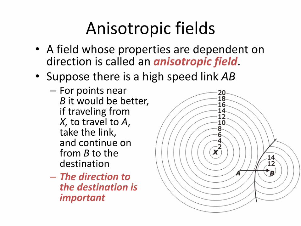
Anisotropic fields • A field whose properties are dependent on

direction is called an anisotropic field. • Suppose there is a high speed link AB

– For points near B it would be better, if traveling from X, to travel to A, take the link, and continue on from B to the destination

– The direction to the destination is important

Spatial autocorrelation

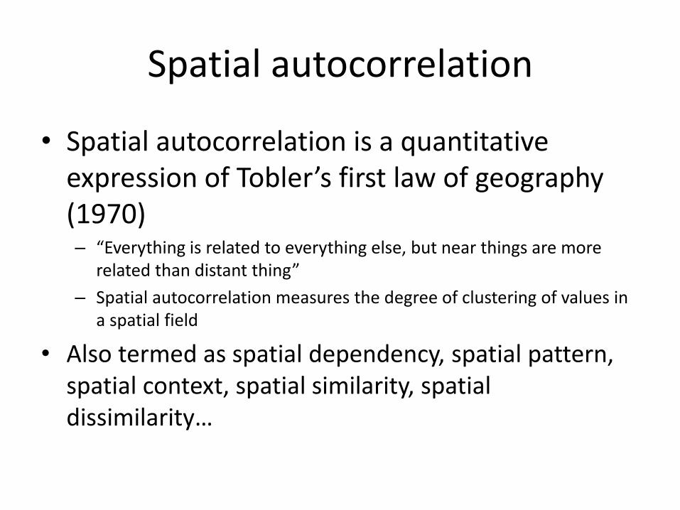
• Spatial autocorrelation is a quantitative expression of Tobler’s first law of geography (1970) – “Everything is related to everything else, but near things are more

related than distant thing”

– Spatial autocorrelation measures the degree of clustering of values in a spatial field

• Also termed as spatial dependency, spatial pattern, spatial context, spatial similarity, spatial dissimilarity…

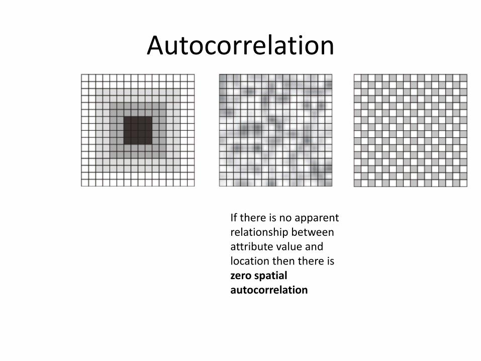
Autocorrelation

If there is no apparent relationship between attribute value and location then there is zero spatial autocorrelation

If like values tend to be located away from each other, then there is negative spatial autocorrelation

If like values

tend to cluster

together,

then the field

exhibits

high positive

spatial

autocorrelation

Representations of Spatial Fields

• Points

• Contours

• Raster/Lattice

• Triangulation (Delaunay Trangulation)

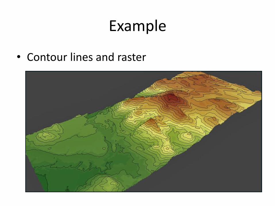
Example

• Contour lines and raster

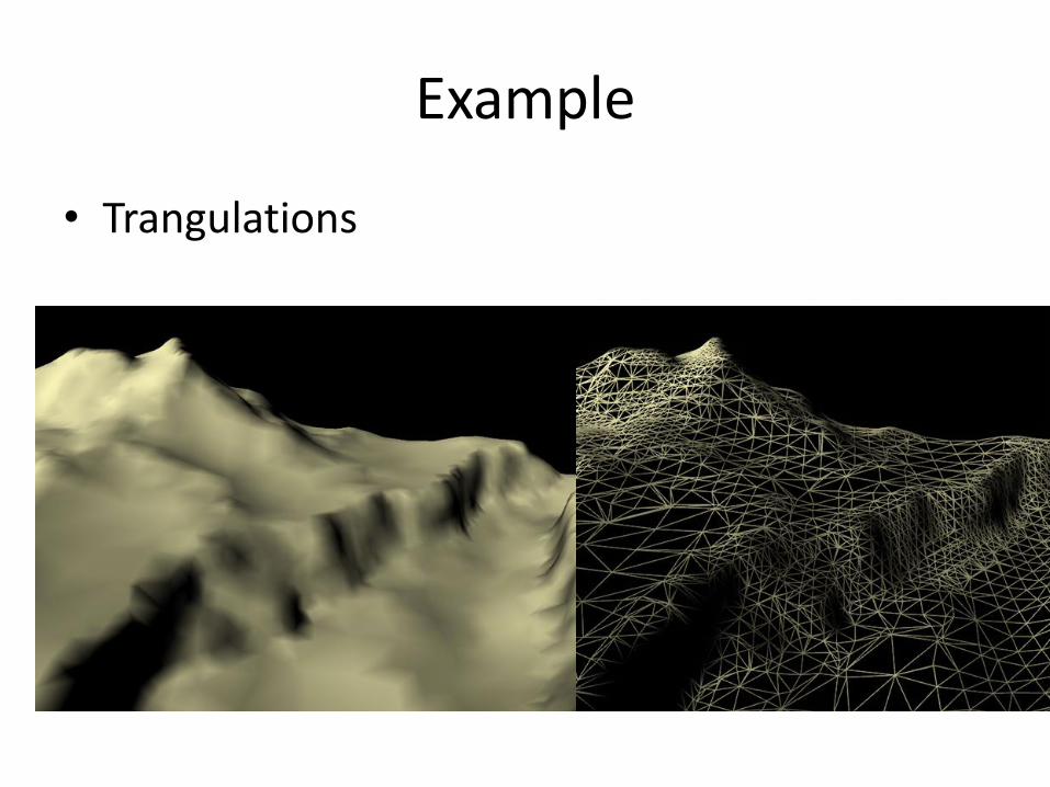
Example

• Trangulations

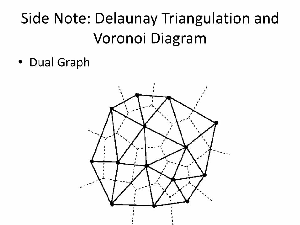
Side Note: Delaunay Triangulation and Voronoi Diagram

• Dual Graph

Operations on fields

• A field operation takes as input one or more fields and returns a resultant field

• The system of possible operations on fields in a field-based model is referred to as map algebra

• Three main classes of operations – Local

– Focal

– Zonal

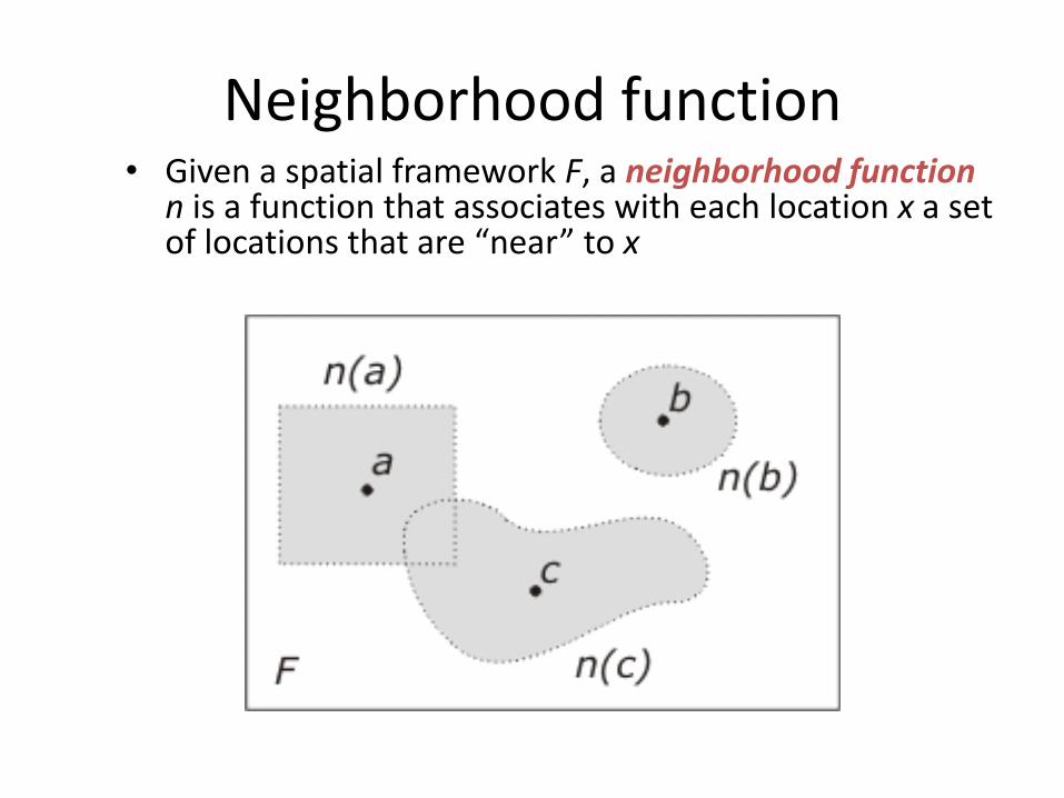
Neighborhood function • Given a spatial framework F, a neighborhood function

n is a function that associates with each location x a set of locations that are “near” to x

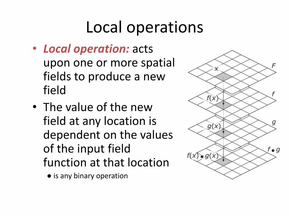
Local operations • Local operation: acts

upon one or more spatial fields to produce a new field

• The value of the new field at any location is dependent on the values of the input field function at that location ● is any binary operation

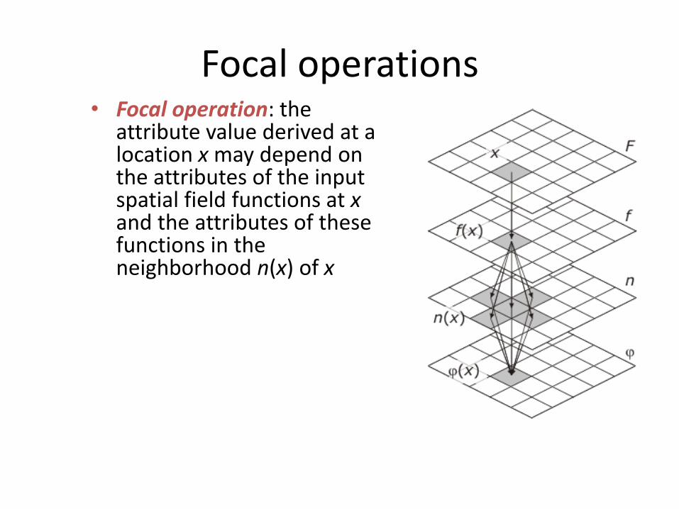
Focal operations • Focal operation: the

attribute value derived at a location x may depend on the attributes of the input spatial field functions at x and the attributes of these functions in the neighborhood n(x) of x

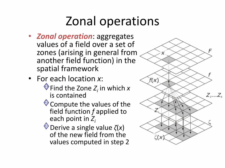
Zonal operations • Zonal operation: aggregates

values of a field over a set of zones (arising in general from another field function) in the spatial framework

• For each location x: 11 Find the Zone Zi in which x

is contained 22 Compute the values of the

field function f applied to each point in Zi

3 Derive a single value ζ(x) of the new field from the values computed in step 2

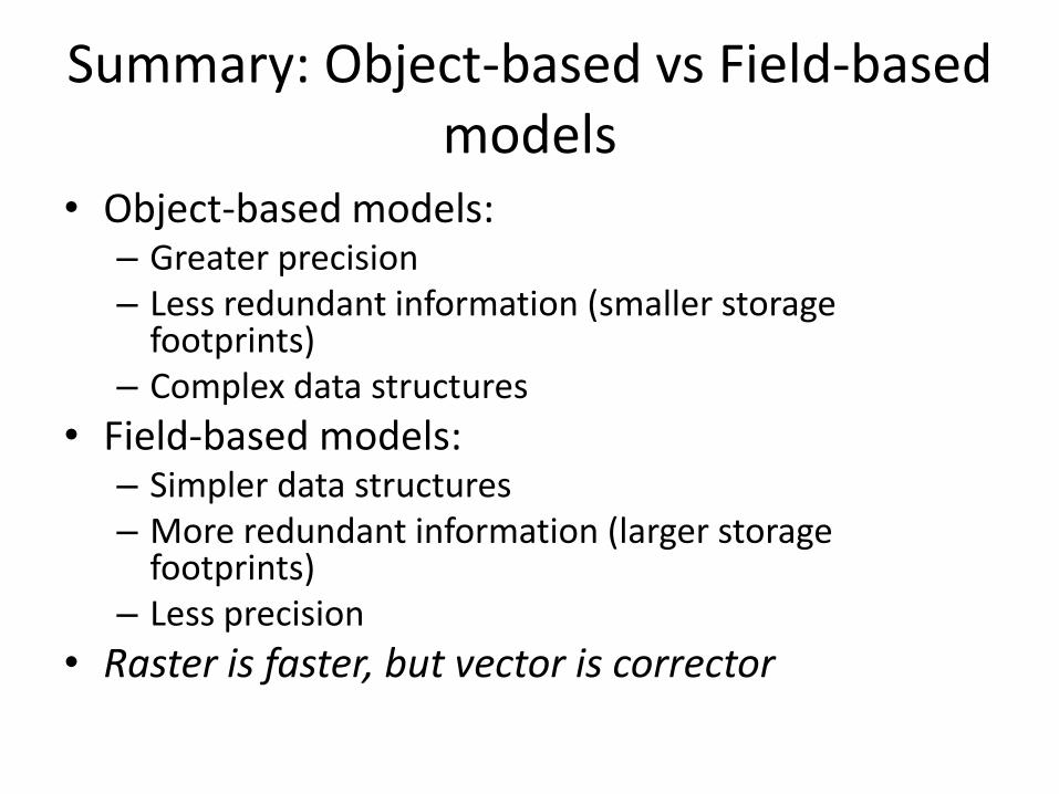
Summary: Object-based vs Field-based models

• Object-based models: – Greater precision – Less redundant information (smaller storage

footprints) – Complex data structures

• Field-based models: – Simpler data structures – More redundant information (larger storage

footprints) – Less precision

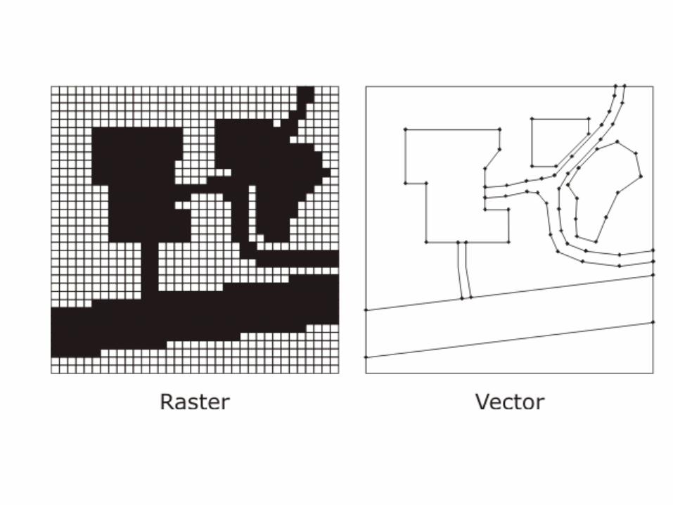
• Raster is faster, but vector is corrector

• End of this topic