Spatial Accounting Methods and the Construction of … · Construction of Spatial Social Accounting Matrices ... factor balances to include origin (supply) and destination ... coincident

Spatial Accounting Methods and theConstruction of Spatial SocialAccounting Matrices

BJARNE MADSEN� & CHRIS JENSEN-BUTLER��

�Institute of Local Government Studies, Nyropsgade, Copenhagen, Denmark, ��Department of Economics,

University of St. Andrews, Fife, Scotland, UK

ABSTRACT The paper examines modifications to Regional Accounts used to construct regional andinterregional Social Accounting Matrices (SAMs). It is argued that as the size of the basic areal unitused in studies declines, more traditional accounting approaches are no longer satisfactory. A three-dimensional spatial approach (termed two-by-two-by-two) to the identification of fundamentaldimensions (commodity and factor market; geographical; and social accounts) has beendeveloped in contrast to the more traditional non-spatial approach (termed two-by-two). Thisinvolves a novel approach using the geographical concepts of place of production for productionactivities, place of residence for institutions, marketplace for commodities and marketplace forfactors. The use of these concepts permits accounting balances to be calculated at the spatiallevel. The theoretical basis of the spatial regional accounting model is presented and an exampleof the construction of a Danish Interregional SAM (SAM-K) is examined. Particular attention isgiven to data requirements, showing that these are much more modest than generally assumed.

KEY WORDS: Interregional SAM, spatial accounting, data requirements

1. Introduction

Developments in spatial accounting and modelling have in part at least, been driven by

policy-makers’ growing interest in regional and local economic performance and inter-

actions with other regions and localities.1 This has promoted increased interest in devel-

opment of regional information systems, where the national accounts-based systems are of

considerable importance. These systems include Regional Accounts (Eurostat, 1996:

Chapter 13), regional versions of satellite accounts (United Nations, 1993: Chapter

XXI) and interregional versions of Social Accounting Matrices (SAM) (United Nations,

1993: Chapter XX; Hewings and Madden, 1995; Round, 1995, 2003; Thorbecke, 1998).

The aim of this paper is to examine the necessary adaptations to Regional Accounts in

Economic Systems Research

Vol. 17, No. 2, 1–24, June 2005

CESR111482 Techset Composition Ltd, Salisbury, U.K. 5/25/2005

Correspondence Address: Bjarne Madsen, AKF, Institute of Local Government Studies, Nyropsgade 37,

DK-Copenhagen, Denmark. Email: [email protected]

0953-5314 Print=1469-5758 Online=05=020001–24 # 2005 Taylor & Francis Group LtdDOI: 10.1080=09535310500114994

order to construct such extended national account based regional information systems.

This includes a novel systematic approach to the treatment of geographical structures

and relations. The paper also provides an example of the implementation of these

adaptations in the case of Denmark.

In National Accounts, a two-by-two registration of economic activities is usually

employed, using the basic division between supply and demand on one dimension and

type of commodity and type of factor on the other, with the nation and Rest of the

World as the geographical units (United Nations, 1993; Eurostat, 1996). If these pro-

duction accounts are divided by industry, an input–output table can be constructed

(United Nations, 1993: Chapter XV; Eurostat, 1996: Chapter 9). If there is a further div-

ision by type of institution, a Social Accounting Matrix (SAM) can be derived (United

Nations, 1993: Chapter XX). These accounts are inherently non-spatial, although this is

usually of little consequence, as the division between the nation and the Rest of the

World is present, and economic dependence on activities in the Rest of the World is

usually relatively limited as is the need for information about spatial structure in relation

to the Rest of the World.

In Regional Accounts (Eurostat, 1996: Chapter 13), the basic geographical unit is the

region rather than the nation and they have a structure which is similar to National

Accounts, although more simple. A number of differences can be noted. First, the focus

of interest is the supply side, where there is no regional supply and demand balance,

although the sum of regional supply is consistent with national totals. Second, there is

no division by commodity and factor. Third, Regional Accounts are limited to recording

production activities by industry and account for some institutional sectors such as house-

holds. Regional Accounts are also non-spatial, though this now becomes a problem as

external links are much more important. This means that two major extensions are necess-

ary if interregional accounting is to be possible. The first extension is to construct

commodity balances and factor balances at the regional level. Whilst this is non-spatial,

it gives the Regional Accounts the same two-by-two structure as the National Accounts.

The second extension is to create the spatial dimension, extending the commodity and

factor balances to include origin (supply) and destination (demand). This in essence

creates a two-by-two-by-two structure. Finally, the term regional is inappropriate as a

number of questions (commuting and shopping for example) can only be properly dealt

with at the sub-regional or local spatial level. In the following, the analysis is as relevant

for the local as for the regional level. Therefore, it is perhaps more appropriate to use the

term local rather than Regional Accounts.

In interregional Social Accounting Matrices, a spatial registration of activities can be

made. Spatial registration implies that activities are registered by place of origin of

inputs and by destination of the outputs. Whilst the step of creating spatial balances is a

natural extension of the principles used in National Accounts to include the spatial dimen-

sion, in the following this spatial registration is based upon the new and systematic use of

the concepts of (i) place of production for production activities where the activity takes

place, (ii) place of residence for institutions, (iii) marketplace for commodities, and

(iv) marketplace for factors.

In this paper, the methods used to set up an interregional SAM for Denmark are

presented, developing ideas found in Madsen and Jensen-Butler (1999, 2002). Based

upon the application of spatial registration of activities the procedure is examined includ-

ing the use of the commodity and factor marketplaces. It is also shown that an

2 B. Madsen & C. Jensen-Butler

interregional Social Accounting Matrix can be set up for countries with limited data

availability.

2. National and Regional Accounts

Regional Accounts are based upon the concepts and accounting principles used in

National Accounts (United Nations, 1993: Chapter XIX; Eurostat, 1996: Chapter 13).

However, for a number of reasons, the national accounting framework is inadequate for

the registration of economic activities in small areas, where economic interaction

between different areas is often intense and the degree of geographical specialisation is

substantial. The national accounting framework is better suited to analyses based upon

well-defined, coincident and relatively closed functional regions.

2.1. National Accounts and the Nation

The conceptual basis of the National Accounts is supply and use, subdivided by

commodity. The mirror image of this concept is the institutional accounts, which are

based upon ownership of the production of the nation, subdivided by type of institution.

This gives a two-by-two structure, with supply and demand on the one dimension and

commodities and factors on the other. The supply of commodities comes either from

domestic production or from imports from abroad, and commodities are produced

either by domestic or by foreign institutions. Demand for commodities is either domestic

demand or foreign exports, and commodities are demanded either by domestic or

foreign institutions. Domestic institutions are, on the one hand, either households or

government, which generate final consumption, and on the other hand, production

units which generate intermediate consumption, gross capital formation and changes

in inventories.

Seen from both the demand and the production side, the geographical units used in

National Accounts are the nation itself and the Rest of the World. A series of rules

have been established to determine whether or not an institution belongs to the nation,

in other words, what is the place of production of the institutional production unit and

the place of residence of the demanding unit.

Using a terminology that is relevant in relation to Regional Accounts, the place of

residence of institutions and, from a production point of view, the place of production

of the institutions, are key concepts used here, which are derived from National Accounts.

The National Accounts are one-dimensional, which means that an institution has one

and only one geographical relation, this being whether the institution is resident or

non-resident.

2.2. National Accounts and Geography

Normally, the concepts of place of residence and place of production are not used in

National Accounts. However, in the context of regional economies they become import-

ant. The smaller the geographical scale, the more necessary it becomes to use the two con-

cepts, as well as to introduce two new concepts, marketplace for commodities and

marketplace for factors. The reason for this multi-dimensionality is that regions become

more specialized as the areal unit for production, place of residence or marketplaces for

Construction of Spatial Social Accounting Matrices 3

commodities and factors becomes geographically smaller. As the size of areal unit

declines, fewer and fewer regions retain all of their functions on all four dimensions.

In National Accounts, this problem also exists, but on a more limited scale. A nation

normally includes all four functions, being place of production, place of residence and

marketplaces for commodities and factors. The transformation from place of production

to place of residence is included in the double entry spatial accounting and is financed

through the balance of payments: incomes from production activities abroad and from

foreigners working inside the national territory (international commuting) are added to

residential institutional incomes. Also, other incomes from abroad and paid abroad are

included in the transformation from place of production to place of residence. This is

not done in conventional National Accounts, where it is only included as a correction

in national disposable income.

The transformation from marketplace for commodities to place of residence is included

in the determination of demand by domestic institution, by subtracting foreign tourists’

demand from total demand. Again, this is a deviation from the single entry principle,

undertaken in order to estimate residential private consumption. Tourists’ demand is

included as part of exports, because it constitutes foreign demand inside the nation (see

Eurostat, 1996: Chapter 3.142). Foreign tourism can be business tourism (treated as part

of intermediate consumption), private tourism (treated as part of private consumption)

and governmental tourism (treated as part of governmental consumption). Tourism is

transformed into exports in two steps. First, the different types of consumption including

tourism are accounted for. In this step the marketplace for commodities is the area in

question. In the second step, tourists’ demand is subtracted from total demand and is

added to exports as one commodity. The demand that remains is, therefore, residential

demand. Similarly, tourists’ consumption abroad, being a separate commodity in

private consumption, is subtracted from demand by type of commodity and added to

imports from abroad. In this way, commodity balances in the first step are accounted

for using the marketplace for commodities, and in the second step they are transferred

to the foreign trade balance by adding domestic tourism abroad to foreign imports and

adding residents’ tourism to foreign exports. Although these problems are managed in

the National Accounts, from the point of view of Regional Accounts this solution is not

satisfactory. Here, an application of all four geographical concepts is necessary.

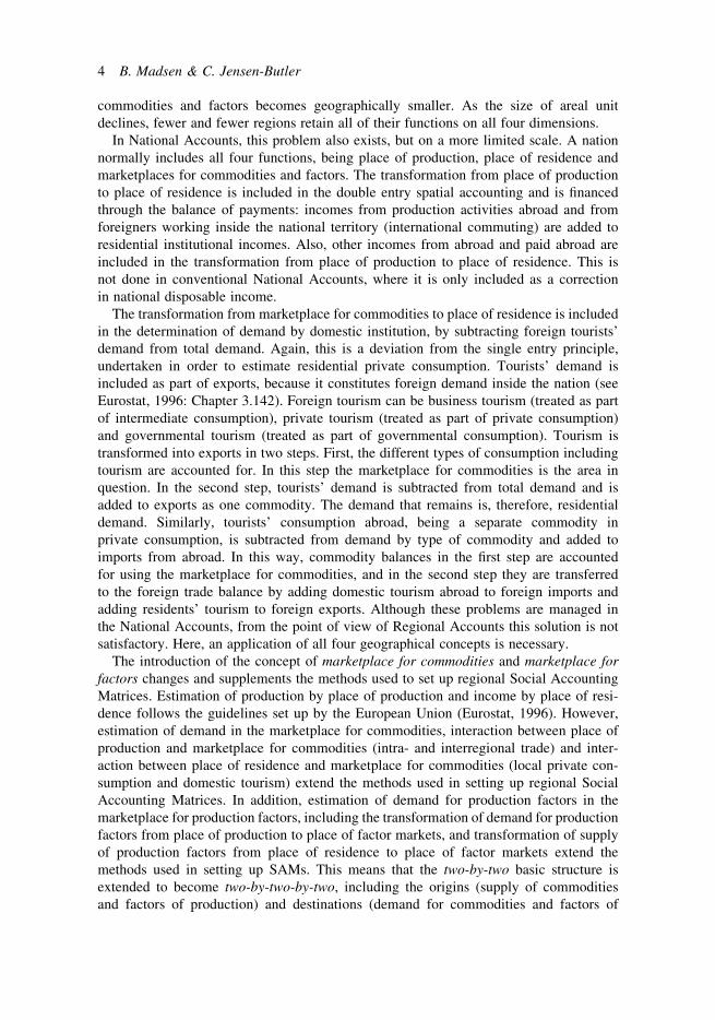
The introduction of the concept of marketplace for commodities and marketplace for

factors changes and supplements the methods used to set up regional Social Accounting

Matrices. Estimation of production by place of production and income by place of resi-

dence follows the guidelines set up by the European Union (Eurostat, 1996). However,

estimation of demand in the marketplace for commodities, interaction between place of

production and marketplace for commodities (intra- and interregional trade) and inter-

action between place of residence and marketplace for commodities (local private con-

sumption and domestic tourism) extend the methods used in setting up regional Social

Accounting Matrices. In addition, estimation of demand for production factors in the

marketplace for production factors, including the transformation of demand for production

factors from place of production to place of factor markets, and transformation of supply

of production factors from place of residence to place of factor markets extend the

methods used in setting up SAMs. This means that the two-by-two basic structure is

extended to become two-by-two-by-two, including the origins (supply of commodities

and factors of production) and destinations (demand for commodities and factors of


production). In the following, this spatial extension of the non-spatial framework is

presented.

2.3. Regional Accounts and Spatial Registration of Economic Activities

In factor markets, supply and demand for production factors are to be found. Demand for

production factors is determined by production at the place of production. In Figure 1,

factor demand by sector is transformed into factor demand by type of production factor.

On the supply side, supply of production factors by type of institution is transformed

into supply by type of production factor. Supply of a production factor is related to the

place of residence of the institution. The factor market is assigned geographically to the

marketplace for factors.

In the case of labour, demand by sector can be transformed into demand by labour group

defined using age, gender and education. Supply of labour is transformed from households

Figure 1. The conceptual basis of spatial social accounts


(institutions) to factor groups (such as age, gender and education). Geographically, the

labour market links the place of production and the place of residence. In the real

world, there are only a few examples of a pure spatially defined labour market, where

the factor marketplace is separated from both the place of production and the place of resi-

dence. An example is the case where workers meet in the morning at a given location,

where the employers hire manpower, and after negotiation, the workers are transported

to the place of production. Normally, the link between place of production and place of

residence is direct in a one-to-one relationship. From this point of view it cannot be

determined whether the place of production or the place of residence is the labour market-

place. However, as the unemployed can be treated as an excess supply of labour, and

unemployment by definition is only assigned to a place of residence, the labour market

can be related to place of residence.

In the commodity market, there is a distinction between place of residence, the market-

place for commodities and place of production. The marketplace for commodities links the

demand for the commodity (from the place of residence to the marketplace for commod-

ities) to the supply of the commodity (from place of production to the marketplace for

commodities). Before the transformation to the marketplace for commodities, the

demand for commodities is transformed from income by institutional group to demand

by commodity. On the supply side, production by sector is transformed from production

by sector into production by commodity and then supply is related geographically to the

marketplace for commodities.

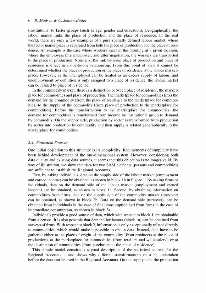
2.4. Statistical Sources

One initial objection to this structure is its complexity. Requirements of simplicity have

been behind development of the one-dimensional system. However, considering both

data quality and existing data sources, it seems that this objection is no longer valid. By

way of illustration, we show that data for two SAM elements (persons and commodities)

are sufficient to establish the Regional Accounts.

First, by asking individuals, data on the supply side of the labour market (employment

and earned income) can be obtained, as shown in block 1b in Figure 1. By asking firms or

individuals, data on the demand side of the labour market (employment and earned

income) can be obtained, as shown in block 1a. Second, by obtaining information on

commodities from firms, data on the supply side of the commodity market (turnover)

can be obtained, as shown in block 2b. Data on the demand side (turnover), can be

obtained from individuals in the case of final consumption and from firms in the case of

intermediate consumption, as shown in block 2a.

Individuals provide a good source of data, which with respect to block 1 are obtainable

from a census. It is also possible that demand for factors (block 1a) can be obtained from

surveys of firms. With respect to block 2, information is only exceptionally related directly

to commodities, which would make it possible to obtain data. Instead, data have to be

gathered either at the place of origin of the commodity (from producers at the place of

production), at the marketplace for commodities (from retailers and wholesalers), or at

the destination of commodities (from purchasers at the place of residence).

This simple model constitutes a good description of the statistical sources for the

Regional Accounts – and shows why different transformations must be undertaken

before the data can be used in the Regional Accounts. On the supply side, the production


account in the Regional Accounts is based upon information from the place of production.

Production statistics will have the format of Make (sector by product) matrices. Statistics

on the labour force, employment and unemployment by type of labour and by type of

household are often based upon census data, sometimes supplemented by other relevant

population data. Finally, demand is, in many cases, most effectively determined at the

place of commodity demand. For example, estimation of private consumption by com-

modity is often based upon VAT statistics, which is related to the marketplace for

commodities.

Before using these statistics in the Regional Accounts, a number of corrections must be

made. In the production statistics, the share of factor income received by non-residential

institutions must be subtracted in order to obtain factor income by place of residence,

which is the key concept in the Regional Accounts. In the demand statistics, demand

from non-residential actors should be subtracted in order to obtain residential demand

for locally produced commodities.

3. Interaction and Regional Accounts

The concept of a balance is fundamental for data construction and accounting. In this

section, the accounting model behind the concept of the commodity balance and the insti-

tutional balance is examined in its most general form. The model, with a few modifications,

is applicable to both regional and national levels. The basic model is transformed into a

two-by-two-by-two spatial model by incorporating the concepts of place of production,

place of residence, place of commodity market and place of the factor market. This

process also represents a transition from a commodity trade balance to an institutional

balance, involving balance of payments and the concept of place of residence.

The accounting balances in a two-by-two non-spatial regional accounting framework

are first presented. This is followed by a discussion of modifications of the general

model with a subdivision into separate balances, these being the private sector balances

and the governmental balances, which corresponds to the balance of payments for the

region. The savings balances can be subdivided into sub-balances, all related to the

place of residence. A discussion of price concepts in the two balances is included later.

Finally, extension to the two-by-two-by-two registration of activities, where sub-balances

are made interregional, is presented and a subdivision of the different balances into

balances for mobile and non-mobile commodities or components of demand is examined.

3.1. A Non-spatial Regional Accounting Model (Two-by-Two Model)

The point of departure for local commodity balances is, on the one hand, data on local

supply (production) and local demand (intermediate consumption, private consumption,

governmental consumption, investments) and on the other hand, the national commodity

balances as represented in the national Make and Use tables. The difference in relation to

the national commodity balance is that interregional imports and exports enter.2 The core

of the regional commodity balance in a SAM is the commodity balance equation for each

region and each commodity, or the total balance:

qPi þ zS;Oi þ zS;Fi ¼ uSi;IC þ uSi;CP þ uSi;CO þ uSi;IN þ zP;Oi þ zP;Fi (1)


where qPi is the gross output by commodity i by place of production P; zS;Oi is the inter-

regional import (O) by commodity by place of commodity market S; zS;Fi is the import

from abroad (F) by commodity by place of commodity market; uSi;IC is the intermediate

consumption (IC) by commodity by place of commodity market; uSi;CP is the private con-

sumption (CP) by commodity by place of commodity market; uSi;CO is the governmental

consumption (CO) by commodity by place of commodity market; uSi;IN is the local invest-

ment (IN) by commodity by place of commodity market; zP;Oi is the interregional export by

commodity by place of production; and zP;Fi is the foreign export by commodity by place

of production.

Equation (1) is formulated explicitly in geographical terms (using P and S). In this case

there is no difference between the national and the regional perspective except that inter-

regional trade has been introduced. From this commodity balance a progression is made to

arrive at a set of institutional balances, corresponding to a process whereby the geographi-

cal dimension is transformed from place of production and commodity marketplace, to

place of residence for regional institutions. This process starts by transforming the per-

spective on production so that it is seen from an institutional place of residence point of

view, as shown in the following equation.

xP � uSIC þ (uS;FIC � uP;FIC )þ (uS;OIC � uP;OIC )þ (hR;F � hP;F)þ (hR;O � hP;O)

¼ uSCP þ uSCO þ uSIN þ (zP;O � zS;O)þ (zP;F � zS;F)

þ (uS;FIC � uP;FIC )þ (uS;OIC � uP;OIC )þ (hR;F � hP;F)þ (hR;O � hP;O) (2)

where xP is gross output by place of production (P); uS;FIC ; uP;FIC ; uS;OIC ; uP;OIC indicate inter-

mediate consumption by foreign (F) or domestic firms (O) in the commodity marketplace

(S) or by place of production (P); hR;F; hP;F; hR;O; hP;O give Gross Value Added (GVA) by

foreign production factors (F) or domestic production factors (O) in place of residence (R)

or by place of production (P).

In equation (2), supply by place of production is transformed into GVA, by place of

residence. This involves a number of steps. First, intermediate consumption is subtracted

both on the supply and use sides of equation (1). Second, correction is made for the pur-

chase of intermediate goods obtained from extra-regional suppliers and the purchase of

intermediate goods in the region by extra-regional producers. Third, a correction is made

for commuting, involving GVA that is generated by institutions resident outside the

region and GVA that is brought into the region by institutions resident in the region

but who are a factor of production that is employed outside the region. Outside the

region is further differentiated into a foreign component and a domestic component.

The result is that the left-hand side becomes the resident institutions’ net earnings.

This left-hand side is a first step towards constructing resident institutions’ saving

balances.

These factor payments from outside the region involve both labour and capital income.

In equation (2), impacts on income or savings from net interest payments from outside

the region should, in principle, also be included, but here they have been left out for

reasons of simplification. Net interest payments could also be subdivided into domestic

and foreign payments. On the right-hand side of the equation (2) the first steps in the

transformation from a trade balance to a balance of payments are taken. This involves


correction of the trade balance using net purchase of intermediate goods and corrections

for commuting.

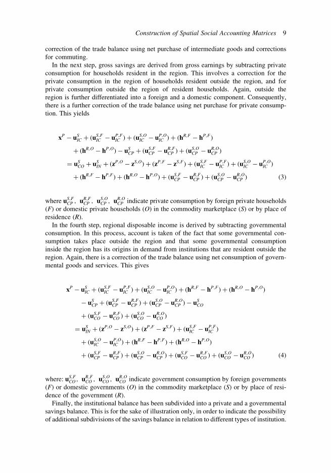
In the next step, gross savings are derived from gross earnings by subtracting private

consumption for households resident in the region. This involves a correction for the

private consumption in the region of households resident outside the region, and for

private consumption outside the region of resident households. Again, outside the

region is further differentiated into a foreign and a domestic component. Consequently,

there is a further correction of the trade balance using net purchase for private consump-

tion. This yields

xP � uSIC þ (uS;FIC � uP;FIC )þ (uS;OIC � uP;OIC )þ (hR;F � hP;F)

þ (hR;O � hP;O)� uSCP þ (uS;FCP � uR;FCP )þ (uS;OCP � uR;OCP )

¼ uSCO þ uSIN þ (zP;O � zS;O)þ (zP;F � zS;F)þ (uS;FIC � uP;FIC )þ (uS;OIC � uP;OIC )

þ (hR;F � hP;F)þ (hR;O � hP;O)þ (uS;FCP � uR;FCP )þ (uS;OCP � uR;OCP ) (3)

where uS;FCP ; uR;FCP ; uS;OCP ; uR;OCP indicate private consumption by foreign private households

(F) or domestic private households (O) in the commodity marketplace (S) or by place of

residence (R).

In the fourth step, regional disposable income is derived by subtracting governmental

consumption. In this process, account is taken of the fact that some governmental con-

sumption takes place outside the region and that some governmental consumption

inside the region has its origins in demand from institutions that are resident outside the

region. Again, there is a correction of the trade balance using net consumption of govern-

mental goods and services. This gives

xP � uSIC þ (uS;FIC � uP;FIC )þ (uS;OIC � uP;OIC )þ (hR;F � hP;F)þ (hR;O � hP;O)

� uSCP þ (uS;FCP � uR;FCP )þ (uS;OCP � uR;OCP )� uSCO

þ (uS;FCO � uR;FCO )þ (uS;OCO � uR;OCO )

¼ uSIN þ (zP;O � zS;O)þ (zP;F � zS;F)þ (uS;FIC � uP;FIC )

þ (uS;OIC � uP;OIC )þ (hR;F � hP;F)þ (hR;O � hP;O)

þ (uS;FCP � uR;FCP )þ (uS;OCP � uR;OCP )þ (uS;FCO � uR;FCO )þ (uS;OCO � uR;OCO ) (4)

where: uS;FCO ; uR;FCO ; uS;OCO ; uR;OCO indicate government consumption by foreign governments

(F) or domestic governments (O) in the commodity marketplace (S) or by place of resi-

dence of the government (R).

Finally, the institutional balance has been subdivided into a private and a governmental

savings balance. This is for the sake of illustration only, in order to indicate the possibility

of additional subdivisions of the savings balance in relation to different types of institution.


This yields

½xP � uPIC þ (hR;F � hP;F)þ (hR;O � hP;O)� uRCP � sR þ tR� þ ½sR � tR � uRCO�

¼ uSIN þ (zP;O � zS;O)þ (zP;F � zS;F)þ (uS;FIC � uP;FIC )þ (uS;OIC � uP;OIC )

þ (hR;F � hP;F)þ (hR;O � hP;O)þ (uS;FCP � uR;FCP )þ (uS;OCP � uR;OCP )

þ (uS;FCO � uR;FCO )þ (uS;OCO � uR;OCO ) (5)

where: sR gives the taxes by place of residence (R), and tR the income transfers by place of

residence.

Whilst at the international level there can be positive or negative residuals in the

balances, this is not the case for the interregional components of the balances. As an

example, the difference in relation to the national commodity balance is that interregio-

nal imports and exports enter, the sum of each being by definition equal. In the construc-

tion of the local commodity balance, the national commodity balance is used. The sum

of each component over all regions is equal to the component at the national level. For

each commodity, the sum of interregional imports equals the sum of interregional

exports.

To summarize, the transformation from place of production to place of residence, gives

regional net savings. The transformation from place of commodity market to place of resi-

dence gives regional net investment plus the balance of payments. This involves the

following central corrections. The first correction is a conventional correction for interre-

gional and foreign trade, where in relation to income, supply from domestic producers is

isolated.

The second correction involves intermediate consumption: a part of intermediate

consumption does not originate from production units producing in the region. For

example, business tourism expenditure included in intermediate consumption by

place of commodity market stems from production units located outside the region.

Therefore, the net surplus on business tourist expenditure is added to both the right

and left sides of the equation, as a reduction in business tourist expenditure for the resi-

dent production units and as an increase in the balance of payments for the tourist

region.

The third correction is to private consumption. If consumption in central regions (with

and above average number of retail centres) is included in residential consumption, private

consumption is overestimated. Therefore, private residential consumption is reduced by

the consumption from non-residents and residential private consumption in other

regions is subtracted when calculating private saving. Similarly, expenditure on domestic

tourism by non-residents is subtracted, and domestic tourist expenditure from residents

outside the region is added. Both corrections on the left-hand side of equation (4) are

added to the balance of payments on the right-hand side of the equation in order to main-

tain the accounting identity.

The fourth correction is for governmental consumption: governmental consumption

with the region as place of commodity market for a government residing outside the

region is subtracted, and governmental consumption of the region itself in other regions

is added. Again a correction to the balance of payments on the right-hand side is added.


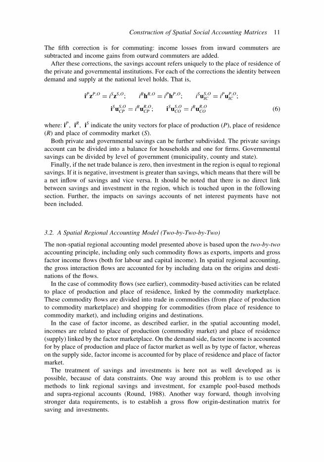
The fifth correction is for commuting: income losses from inward commuters are

subtracted and income gains from outward commuters are added.

After these corrections, the savings account refers uniquely to the place of residence of

the private and governmental institutions. For each of the corrections the identity between

demand and supply at the national level holds. That is,

iPzP;O ¼ iSzS;O; iRhR;O ¼ iPhP;O; iSuS;OIC ¼ iPuP;OIC ;

iSuS;OCP ¼ iRuR;OCP ; iSuS;OCO ¼ iRuR;OCO (6)

where: iP; iR; iS indicate the unity vectors for place of production (P), place of residence

(R) and place of commodity market (S).

Both private and governmental savings can be further subdivided. The private savings

account can be divided into a balance for households and one for firms. Governmental

savings can be divided by level of government (municipality, county and state).

Finally, if the net trade balance is zero, then investment in the region is equal to regional

savings. If it is negative, investment is greater than savings, which means that there will be

a net inflow of savings and vice versa. It should be noted that there is no direct link

between savings and investment in the region, which is touched upon in the following

section. Further, the impacts on savings accounts of net interest payments have not

been included.

3.2. A Spatial Regional Accounting Model (Two-by-Two-by-Two)

The non-spatial regional accounting model presented above is based upon the two-by-two

accounting principle, including only such commodity flows as exports, imports and gross

factor income flows (both for labour and capital income). In spatial regional accounting,

the gross interaction flows are accounted for by including data on the origins and desti-

nations of the flows.

In the case of commodity flows (see earlier), commodity-based activities can be related

to place of production and place of residence, linked by the commodity marketplace.

These commodity flows are divided into trade in commodities (from place of production

to commodity marketplace) and shopping for commodities (from place of residence to

commodity market), and including origins and destinations.

In the case of factor income, as described earlier, in the spatial accounting model,

incomes are related to place of production (commodity market) and place of residence

(supply) linked by the factor marketplace. On the demand side, factor income is accounted

for by place of production and place of factor market as well as by type of factor, whereas

on the supply side, factor income is accounted for by place of residence and place of factor

market.

The treatment of savings and investments is here not as well developed as is

possible, because of data constraints. One way around this problem is to use other

methods to link regional savings and investment, for example pool-based methods

and supra-regional accounts (Round, 1988). Another way forward, though involving

stronger data requirements, is to establish a gross flow origin-destination matrix for

saving and investments.


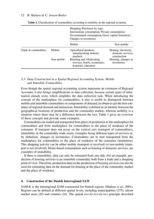
3.3. Data Construction in a Spatial Regional Accounting System: Mobile

and Immobile Commodities

Even though the spatial regional accounting system represents an extension of Regional

Accounts, it also brings simplifications in data collection, because certain types of infor-

mation already exist, which simplifies the data collection task. When introducing the

concept of the marketplace for commodities, it also is useful to distinguish between

mobile and immobile commodities or components of demand, in obtain to get the best esti-

mates of regional demand and interaction. Immobility is defined as an identity between the

geographical locations of production and the commodity market, whereas mobility is a

situation where there may be a difference between the two. Table 1 gives an overview

of these concepts and provide some examples.

Commodities are traded and transported from place of production to the marketplace for

commodities and from marketplace for commodities to the place of residence of the

consumer. If transport does not occur on the vertical axis (transport of commodities),

immobility in the commodity trade exists, examples being different types of services or,

by definition, changes in inventories. Commodities are in turn transported from the

marketplace for commodities to the place of residence of the consumer (institution).

This shopping activity can be either mobile (transport is involved) or non-mobile (trans-

port is not involved). Home-based consumption such as housing or domestic services, are

examples of immobility.

If there is immobility, data can only be estimated from one side. For an example, pro-

duction of housing services is an immobile commodity both from a trade and a shopping

point of view. Therefore, production data on the production of housing services can also be

used for estimating data on the demand for housing at the place of the commodity market

and the place of residence.

4. Construction of the Danish Interregional SAM

SAM-K is the interregional SAM constructed for Danish regions (Madsen et al., 2001).

Regions can be defined at different spatial levels, including municipalities (275), labour

market areas (45) and counties (16). The spatial two-by-two-by-two principle described

Table 1. Classification of commodities according to mobility in the regional economy

Shopping/Purchases by type:

Intermediate consumption/Private consumption/Governmental consumption/Gross capital formation/Changes in inventories

Mobile Non-mobile

Trade in commodities Mobile Agricultural products,manufacturing industryproducts

Heating, electricity,domestic services,construction

Non-mobile Retailing and wholesaling,services, hotels, restaurants,hospitals, education

Housing, changes ininventories


above has been the guiding principle for the construction of SAM-K. It is, in principle,

designed using the structure shown in Figure 1, being based upon the double spatial

entry principle or extended regional accounts (two-by-two-by-two), rather than the non-

spatial regional accounting principles (two-by-two).

The structure of SAM-K follows the basic interregional SAM (Figure 1) with: factor

markets and commodity markets; demand and supply; origin (supply) and destination

(demand); and incorporating some simplifications and extensions. The basic interregional

SAM must be adjusted in order to take into account the nature of the statistics, data collec-

tion methods and the structure of the regional economy. On one hand, the model must be

broken down and in other aspects it must be merged.

First, the concept of the marketplace for factors does not correspond in general to

reality, as noted above. In practice, the place of residence of the production factor (such

as labour) can be interpreted as both place of residence and marketplace for factors.

Only in very few cases does a geographically defined factor market exist. From a data

collection point of view, only registration of place of residence and place production is

possible. Therefore, the marketplace for factors has been excluded from SAM-K.

Second, only factor income from labour receives a full treatment. In Denmark, regional

data on capital income only exist by place of production. Data on interregional transfer of

capital income are still lacking, which makes a comparable treatment to commuting flows

involving labour income impossible and identification of the marketplace for capital

income difficult to develop. Future developments with respect to treatment of savings

and investments and identification of marketplaces for these could include the use of

pooling methods or identification of gross flows, referred to above.

Third, there is a need to keep track of economic interactions between institutions.

Interaction between households and the governmental sector is important in order to

describe the economic strength of households, for example measured by disposable

income of households including income transfers from government and the subtraction

of taxes. From a data collection point of view, this information does not create any

special problems as these payments are assigned to individuals.

Fourth, consumption by institutions (households) both from a decision-making and data

collection point of view must be divided into two nested steps. First, consumption is deter-

mined at a high level of aggregation, for example food, clothing, transport etc. In the next

step, the consumption bundles are further divided into specific commodities. From a

decision-making point of view, both the first and second steps are a part of the household

decision problem, the sellers (the retail sector) reflecting demand from the households.

From a data collection point of view the two steps are also related to two data sources:

(i) household expenditure surveys, which often include information at a relatively

aggregate level, where household consumption is assigned to the place of residence;

and (ii) the retail sector and producers (who pay specific commodity taxes) make a sub-

stantial contribution to detailed data on demand, usually through information related to

the value added tax and commodity taxes. The same is the case for other types of

final demand, such as governmental consumption and gross capital formation, where

information is available in the marketplace for commodities.

Fifth, different price concepts are included in different accounts, reflecting the fact that

different data sources use different price concepts. In the account for goods and services,

total expenditures are measured in market prices. Supply of commodities entering the

goods and services account is accounted for in basic prices. Basic prices are defined as


the value of production at the factory, not including net commodity taxes paid by the pro-

ducer. Going from market/buyers prices to basic prices at the place of commodity market

involves subtraction of commodity taxes and trade margins, where trade margins also are

part of the commodity account.

Sixth, in general, the SAM is constructed using current prices. However, for data con-

cerning production of commodities, values have been deflated to fixed prices at a low level

of disaggregation, using national price data. This extension permits analysis of real

changes in production over time.

In addition, there are some extensions, such as the transformation from basic prices to

market prices and the transformation from institutions to commodities, which in the

Danish interregional SAM is divided into two steps: from institutions to components

and from components to commodities. Despite this deviation, the Danish system can be

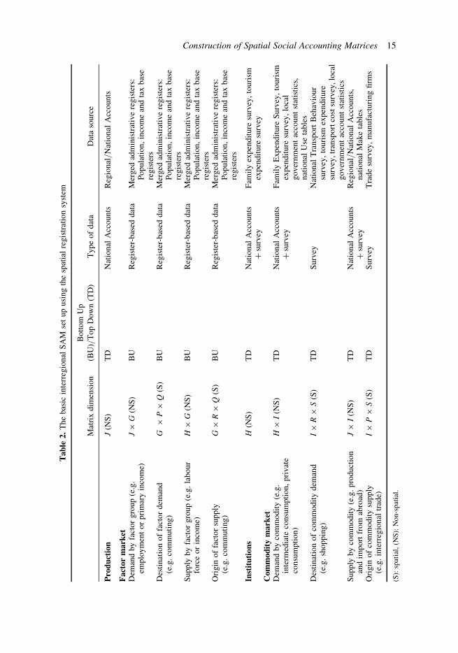
represented in a basic four-element system, as shown in Table 2.

4.1. The Basic Interregional SAM and SAM-K

Despite these conceptual deviations, the basic interregional SAM forms a useful frame-

work to describe the data construction procedures and sources used in building SAM-K.

Table 2 contains information on the dimensions of SAM-K and the procedures and

content of the matrices used to build SAM-K. These cover economic activities related

to production and institutions as well as the regional commodity and factor markets.

The economic activities associated with production and institutions follow the convention-

al non-spatial format in the National Accounts. Here the information on production and

institutions consists of vectors subdivided by sectors (using axis J) and by institutions

(using axis H). Economic activity associated with the factor and commodity markets

builds upon the spatial accounting principle.

The accounts for the factor market have the following structure: (i) the factor market has

been divided into supply and demand; (ii) demand for factors of production has been trans-

formed from sectors using axis J to factor groups using axis G and supply of factors of

production has been transformed from Institutions using axis H to factor groups using

axis G; and (iii) demand for factors of production has been transformed from place of

production using axis P to place of factor markets using axis Q and the supply of

factors has been transformed from place of residence using axis R to place of factor

market, using axis Q.

Similar transformations take place in the commodity market, where the accounts for the

commodity market have the following structure: (i) the commodity market has been

divided into supply and demand; (ii) demand for commodities has been transformed

from institutions using axis H to commodities using axis I and supply of commodities

has been transformed from sectors using axis J to commodities using axis I; and (iii)

the demand for commodities has been transformed from place of residence using axis R

to place of commodity market using axis S and the supply of commodities has been trans-

formed from place of production using axis P to place of commodity market, using axis S.

Items (ii) and (iii) in both markets represent collection of data in matrix rather than the

vector format, which is used in the non-spatial Regional Accounts. Item (ii) represents a

transformation between SAM categories and item (iii) is a geographical specification of

the origin and destination of demand and supply in both markets. In the following, con-

struction of the Danish SAM is described with reference to entering data into these


Table

2.

Th

eb

asic

inte

rreg

ion

alS

AM

set

up

usi

ng

the

spat

ial

reg

istr

atio

nsy

stem

Mat

rix

dim

ensi

on

Bo

tto

mU

p

(BU

)/T

op

Do

wn

(TD

)T

yp

eo

fd

ata

Dat

aso

urc

e

Production

J(N

S)

TD

Nat

ion

alA

cco

un

tsR

egio

nal/N

atio

nal

Acc

ou

nts

Factormarket

Dem

and

by

fact

or

gro

up

(e.g

.em

plo

ym

ent

or

pri

mar

yin

com

e)J�

G(N

S)

BU

Reg

iste

r-b

ased

dat

aM

erg

edad

min

istr

ativ

ere

gis

ters

:P

op

ula

tio

n,

inco

me

and

tax

bas

ere

gis

ters

Des

tin

atio

no

ffa

cto

rd

eman

d(e

.g.

com

mu

tin

g)

G�

P�

Q(S

)B

UR

egis

ter-

bas

edd

ata

Mer

ged

adm

inis

trat

ive

reg

iste

rs:

Po

pu

lati

on

,in

com

ean

dta

xb

ase

reg

iste

rsS

up

ply

by

fact

or

gro

up

(e.g

.la

bo

ur

forc

eo

rin

com

e)H�

G(N

S)

BU

Reg

iste

r-b

ased

dat

aM

erg

edad

min

istr

ativ

ere

gis

ters

:P

op

ula

tio

n,

inco

me

and

tax

bas

ere

gis

ters

Ori

gin

of

fact

or

sup

ply

(e.g

.co

mm

uti

ng

)G�

R�

Q(S

)B

UR

egis

ter-

bas

edd

ata

Mer

ged

adm

inis

trat

ive

reg

iste

rs:

Po

pu

lati

on

,in

com

ean

dta

xb

ase

reg

iste

rs

Institutions

H(N

S)

TD

Nat

ion

alA

cco

un

tsþ

surv

eyF

amil

yex

pen

dit

ure

surv

ey,

tou

rism

exp

end

itu

resu

rvey

Commoditymarket

Dem

and

by

com

mo

dit

y(e

.g.

inte

rmed

iate

con

sum

pti

on

,p

riv

ate

con

sum

pti

on

)

H�

I(N

S)

TD

Nat

ion

alA

cco

un

tsþ

surv

eyF

amil

yE

xp

end

itu

reS

urv

ey,

tou

rism

exp

end

itu

resu

rvey

,lo

cal

go

ver

nm

ent

acco

un

tst

atis

tics

,n

atio

nal

Use

tab

les

Des

tin

atio

no

fco

mm

od

ity

dem

and

(e.g

.sh

op

pin

g)

I�

R�

S(S

)T

DS

urv

eyN

atio

nal

Tra

nsp

ort

Beh

avio

ur

surv

ey,

tou

rism

exp

end

itu

resu

rvey

,tr

ansp

ort

cost

surv

ey,lo

cal

go

ver

nm

ent

acco

un

tst

atis

tics

Su

pp

lyb

yco

mm

od

ity

(e.g

.p

rod

uct

ion

and

imp

ort

fro

mab

road

)J�

I(N

S)

TD

Nat

ion

alA

cco

un

tsþ

surv

eyR

egio

nal/N

atio

nal

Acc

ou

nts

,n

atio

nal

Mak

eta

ble

sO

rig

ino

fco

mm

od

ity

sup

ply

(e.g

.in

terr

egio

nal

trad

e)I�

P�

S(S

)T

DS

urv

eyT

rad

esu

rvey

,m

anu

fact

uri

ng

firm

s

(S):

spat

ial,

(NS

):N

on

-sp

atia

l.


vectors (non-spatial) and matrices (spatial). Full documentation of the principles used to

set up the interregional SAM for Denmark is provided in Madsen et al. (2001)

4.2. Data on Regional Production, Incomes and Employment

by Institution (Regional: Non-spatial)

Data on production by 275 municipalities and 130 sectors is provided by Statistics

Denmark, following the principles set out in Eurostat (1996), and is documented in

detail in Madsen et al. (2001: Chapter 4). Basically, the point of departure is data from

the National Accounts by sector, which are used together with different sources to

break down the national data to regional data. The methodologies can be divided into

use of Top Down (TD) methods where the sum of the regional data is scaled to be consist-

ent with national data and Bottom Up (BU) data where the national sum is by definition

equal to the sum of the regional values. Further sources can be divided into statistics

for administrative purposes and statistics from surveys (usually undertaken regularly by

a government body). Finally there is the issue of whether the statistics are based on popu-

lation or samples. All in all, ten different methods are used.

Data on institutions (Madsen et al., 2001: Chapter 5) cover at present households and

include data on earned income, income transfers, taxes, unemployment and employment,

for 275 municipalities and four types of household. The sources of this data include admin-

istrative registers, which provide data on income, taxes and employment. The data is

Bottom Up, with full population coverage. A central variable is disposable income

(related to commodity purchase).

4.3. Data on Factor Markets (Regional: Spatial and Non-spatial)

Madsen et al. (2001: Chapter 5) describe these data sources in more detail. Data on

production factors include labour force, income and employment. The data are Bottom

Up and are obtained from administrative registers, providing data by category on:

sectors, factors (distinguishing two gender types, seven age classes, five types of edu-

cation, and four categories of household composition), place of production and place of

factor market (residence). The matrices are filled out with data described above using

bottom up principles. Demand goes from place of production to place of residence and

supply goes in the reverse direction.

4.4. Data on Commodity Markets (Regional: Non-spatial)

The procedures for estimating commodity balances are described in Madsen et al. (2001:

Chapters 6–9). First the estimation of supply (in the next section) and demand (in the

section after) are described, after which total intra- and interregional trade by commodity

is estimated. The geographical patterns of interregional trade flows by commodity are then

determined.

For the construction of commodity balances and interregional flows the approach uses

regional data on production and demand, which is combined with national assumptions on

commodity composition of production and demand. The assumption relating to the

national commodity composition is the reason why the approach is termed national. In

the construction of the local commodity balances, including the individual components,


which enter into the commodity balance to be found in equation (1), the national commod-

ity balance is used (the Top Down approach).

The commodity balances are determined for a number of Danish regions, typically 16

counties plus one extra artificial county, containing economic activities, which cannot

easily be allocated to a geographical location (production of crude oil, maritime transport,

etc). The 17 regions have been aggregated from the 275 municipalities, which is the lowest

level of disaggregation possible in the Danish interregional SAM. The commodity bal-

ances at regional level are estimated for 20–30 commodities, which are aggregated

from the available data on 130 commodities.

4.5. Regional Supply by Commodity (Regional: Non-spatial)

Supply of commodities consists of local production of commodities, imports of commod-

ities from abroad and interregional commodity import. Local production of commodities

is estimated using local sectoral values for gross output combined with sector-specific

information on the composition of gross output by commodity (Make matrix).

qPi ¼ ij DNAT

WxP (7)

where ij is an aggregation vector by sector j; DNAT is gross output by commodity i as a

share of gross output by sector j at the national level; and xP is gross output by sector

by place of production P.

The data on gross output by sector and by municipality are obtained from Statistics

Denmark (described earlier). Gross output is in basic prices (by definition) and in both

fixed and current prices. Data on the composition of gross output by commodity originate

from the national Make matrices. The basic approach to estimation of international

imports by commodity at the local level is to multiply local demand for a commodity

by a (national) import share (of the aggregated local demand). Local demand is calculated

as the sum of local intermediate and local final demand in basic prices. It is assumed that

there is no major deviation between national and local import shares.

zS;Fi ¼ zSi WDF;NATi (8)

where zS;Fi are international imports by commodity i by municipality S; zSi is local demand

by commodity and by municipality; and DF;NATi gives the import share by commodity at

the national level.

Technically, imports are divided into imports for the domestic market and imports for

re-export, the latter being smaller than the former. Estimation of interregional imports by

commodity is described in the section after next.

4.6. Regional Demand by Commodity (Regional: Non-spatial)

Demand for commodities in any locality consists of local demand, foreign exports and

interregional exports. Local demand, by region, by commodity and in total, is, by defi-

nition:

zSi ¼ uSi;IC þ uSi;CP þ uSi;CPR þ uSi;COR þ uSi;CO þ uSi;IR þ uSi;IL (9)


where: zSi is local demand by place of commodity market S and by commodity i; uSi;IC is

intermediate consumption by place of commodity market and by commodity; uSi;CP gives

private individual consumption expenditure by place of commodity market and by com-

modity; uSi;CPR is private consumption in membership organisations by place of commodity

market and by commodity; uSi;COR is governmental individual consumption expenditure by

place of commodity market and by commodity; uSi;CO is governmental collective consump-

tion expenditure by place of commodity market and by commodity; uSi;IR is gross fixed

capital formation by place of commodity market and by commodity; and uSi;IL gives the

changes in inventories by place of commodity market and by commodity.

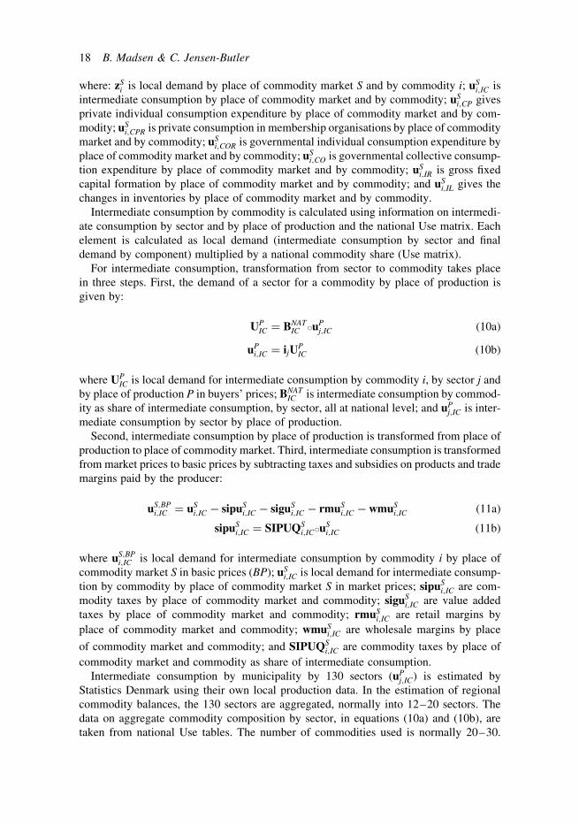
Intermediate consumption by commodity is calculated using information on intermedi-

ate consumption by sector and by place of production and the national Use matrix. Each

element is calculated as local demand (intermediate consumption by sector and final

demand by component) multiplied by a national commodity share (Use matrix).

For intermediate consumption, transformation from sector to commodity takes place

in three steps. First, the demand of a sector for a commodity by place of production is

given by:

UPIC ¼ BNAT

IC WuPj;IC (10a)

uPi;IC ¼ ijUPIC (10b)

where UPIC is local demand for intermediate consumption by commodity i, by sector j and

by place of production P in buyers’ prices; BNATIC is intermediate consumption by commod-

ity as share of intermediate consumption, by sector, all at national level; and uPj;IC is inter-

mediate consumption by sector by place of production.

Second, intermediate consumption by place of production is transformed from place of

production to place of commodity market. Third, intermediate consumption is transformed

from market prices to basic prices by subtracting taxes and subsidies on products and trade

margins paid by the producer:

uS;BPi;IC ¼ uSi;IC � sipuSi;IC � siguSi;IC � rmuSi;IC � wmuSi;IC (11a)

sipuSi;IC ¼ SIPUQSi;ICWuSi;IC (11b)

where uS;BPi;IC is local demand for intermediate consumption by commodity i by place of

commodity market S in basic prices (BP); uSi;IC is local demand for intermediate consump-

tion by commodity by place of commodity market S in market prices; sipuSi;IC are com-

modity taxes by place of commodity market and commodity; siguSi;IC are value added

taxes by place of commodity market and commodity; rmuSi;IC are retail margins by

place of commodity market and commodity; wmuSi;IC are wholesale margins by place

of commodity market and commodity; and SIPUQSi;IC are commodity taxes by place of

commodity market and commodity as share of intermediate consumption.

Intermediate consumption by municipality by 130 sectors (uPj;IC) is estimated by

Statistics Denmark using their own local production data. In the estimation of regional

commodity balances, the 130 sectors are aggregated, normally into 12–20 sectors. The

data on aggregate commodity composition by sector, in equations (10a) and (10b), are

taken from national Use tables. The number of commodities used is normally 20–30.


Shopping for intermediate consumption is estimated using transport survey data.

Estimation of commodity taxes and trade margins is based upon national commodity

tax rates and national shares in the case of wholesaling margins and regional shares in

the case of retail margins. The corresponding calculations are made for the components

of final demand.

Exports to the Rest of World are distributed as exports from localities in proportion to

gross output by commodity, by place of production. The basic approach to estimation of

international exports is to multiply gross output with a national export share:

zP;Fi ¼ qPi WBF;NATi (12)

where zP;Fi are international exports by commodity i by place of production P; and BF;NATi

is the share of exports in production by commodity at the national level.

The national approach in this field also relies on the assumption that location close to a

border does not affect export shares. Modification of this assumption would have to be

based upon survey data. Technically, exports are divided into exports produced domesti-

cally and re-exports, the latter imported from abroad. Interregional export by commodity

is dealt with in the following section.

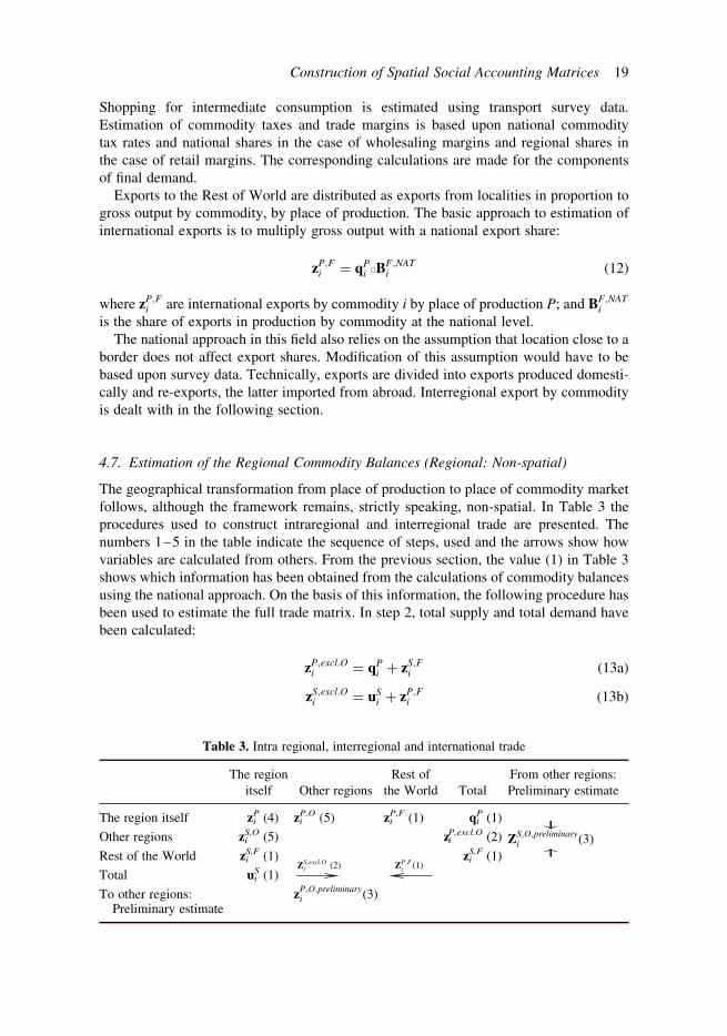
4.7. Estimation of the Regional Commodity Balances (Regional: Non-spatial)

The geographical transformation from place of production to place of commodity market

follows, although the framework remains, strictly speaking, non-spatial. In Table 3 the

procedures used to construct intraregional and interregional trade are presented. The

numbers 1–5 in the table indicate the sequence of steps, used and the arrows show how

variables are calculated from others. From the previous section, the value (1) in Table 3

shows which information has been obtained from the calculations of commodity balances

using the national approach. On the basis of this information, the following procedure has

been used to estimate the full trade matrix. In step 2, total supply and total demand have

been calculated:

zP;excl:Oi ¼ qPi þ zS;Fi (13a)

zS;excl:Oi ¼ uSi þ zP;Fi (13b)

Table 3. Intra regional, interregional and international trade

The region

itself Other regions

Rest of

the World Total

From other regions:

Preliminary estimate

The region itself ziP (4) zi

P,O (5) ziP,F (1) qi

P (1)

ZS;O;preliminaryi (3)

#

"

Other regions ziS,O (5) zi

P,excl.O (2)

Rest of the World ziS,F (1) zi

S,F (1)

Total uiS (1) !

ZS;excl:Oi

(2)

ZP;Fi

(1)

To other regions:Preliminary estimate

zP;O;preliminaryi (3)


where zP;excl:Oi is total supply, excluding interregional imports, by commodity i; and

zS;excl:Oi is total demand, excluding interregional exports, by commodity.

In step 3 total supply, excluding interregional imports, has been compared to total

demand, excluding interregional exports, in order to calculate a preliminary value for

interregional imports and exports by commodity:

if zP;excl:Oi . zS;excl:Oi then zP;O;preliminaryi ¼ zP;excl:Oi � zS;excl:Oi (14a)

if zP;excl:Oi � zS;excl:Oi then zS;O;preliminaryi ¼ zS;excl:Oi � zP;excl:Oi (14b)

where zP;O;preliminaryi are interregional exports by commodity i – preliminary values; and

zS;O;preliminaryi are interregional imports by commodity – preliminary values.

In the fourth step, intra regional supply and demand have been calculated on the basis of

the preliminary values of interregional import and export by commodity:

zP;preliminaryi ¼ qi � zP;Fi � z

P;O;preliminaryi (15)

where zP;preliminaryi is intra regional supply by commodity i – preliminary value.

In the last step, two-way trade (cross hauling) has been included in the estimation of

interregional trade flows:

if zP;O;preliminaryi ¼ 0 then zP;Oi ¼ z

P;O;preliminaryi þ g � qPi and

zS;Oi ¼ zS;O;preliminaryi þ g � qPi (16a)

if zS;O;preliminaryi ¼ 0 then zS;Oi ¼ z

S;O;preliminaryi þ g � uSi and

zP;Oi ¼ zP;O;preliminaryi þ g � uSi (16b)

where zP;Oi is interregional export by commodity i; g is the cross-hauling parameter (see

below); and zS;Oi is interregional import by commodity.

The exogenous variable g is a cross-hauling parameter that varies between groups of

commodities and determines the additional interregional trade that is due to cross-

hauling. Note that g is not equal to the share of the region’s production that meets its

own demand, as the level of cross-hauling depends on local production and local

demand, respectively. The proportion of the region’s production that meets its own

demand is the result of the estimation procedure. If the region is a net supplier, the

additional interregional trade (cross-hauling) is calculated by multiplying local production

by g. If the region is a net demander, the local demand is multiplied by g. In Jensen-Butler

et al. (2004), a trade survey is used to estimate g for seven industrial commodities.

Even though the equations for calculation of the different balances are the same for all

commodities, there is also an implicit difference in the treatment of mobile and immobile

commodities. Immobile commodities are characterised by the fact that local demand and

local production are equal, being located in the same geographical unit. This is a definition

that can be compared with tradable and non-tradable commodities. Tradable commodities

are those that compete with the same or similar products from the Rest of the World.

Non-tradable commodities are those that are protected from this competition, either


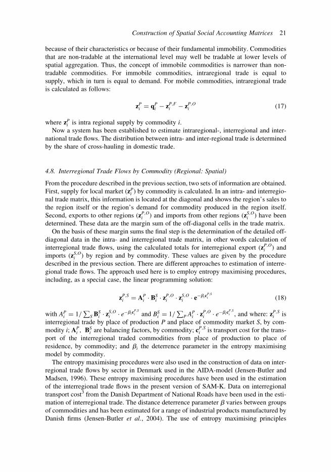
because of their characteristics or because of their fundamental immobility. Commodities

that are non-tradable at the international level may well be tradable at lower levels of

spatial aggregation. Thus, the concept of immobile commodities is narrower than non-

tradable commodities. For immobile commodities, intraregional trade is equal to

supply, which in turn is equal to demand. For mobile commodities, intraregional trade

is calculated as follows:

zPi ¼ qPi � zP;Fi � zP;Oi (17)

where zPi is intra regional supply by commodity i.

Now a system has been established to estimate intraregional-, interregional and inter-

national trade flows. The distribution between intra- and inter-regional trade is determined

by the share of cross-hauling in domestic trade.

4.8. Interregional Trade Flows by Commodity (Regional: Spatial)

From the procedure described in the previous section, two sets of information are obtained.

First, supply for local market (zPi ) by commodity is calculated. In an intra- and interregio-

nal trade matrix, this information is located at the diagonal and shows the region’s sales to

the region itself or the region’s demand for commodity produced in the region itself.

Second, exports to other regions (zP;Oi ) and imports from other regions (zS;Oi ) have been

determined. These data are the margin sum of the off-diagonal cells in the trade matrix.

On the basis of these margin sums the final step is the determination of the detailed off-

diagonal data in the intra- and interregional trade matrix, in other words calculation of

interregional trade flows, using the calculated totals for interregional export (zP;Oi ) and

imports (zS;Oi ) by region and by commodity. These values are given by the procedure

described in the previous section. There are different approaches to estimation of interre-

gional trade flows. The approach used here is to employ entropy maximising procedures,

including, as a special case, the linear programming solution:

zP;Si ¼ APi � B

Si � z

P;Oi � z

S;Oi � e

�bicP;Si (18)

with APi ¼ 1=

PS B

Si � z

S;Oi � e

�bicP;Si and BS

i ¼ 1=P

P APi � z

P;Oi � e

�bicP;Si , and where: zP;Si is

interregional trade by place of production P and place of commodity market S, by com-

modity i; APi ; BS

i are balancing factors, by commodity; cP;Si is transport cost for the trans-

port of the interregional traded commodities from place of production to place of

residence, by commodity; and bi the deterrence parameter in the entropy maximising

model by commodity.

The entropy maximising procedures were also used in the construction of data on inter-

regional trade flows by sector in Denmark used in the AIDA-model (Jensen-Butler and

Madsen, 1996). These entropy maximising procedures have been used in the estimation

of the interregional trade flows in the present version of SAM-K. Data on interregional

transport cost3 from the Danish Department of National Roads have been used in the esti-

mation of interregional trade. The distance deterrence parameter b varies between groups

of commodities and has been estimated for a range of industrial products manufactured by

Danish firms (Jensen-Butler et al., 2004). The use of entropy maximising principles


involving a distance deterrence function implies that distance related transportation costs

play a central role in determining the pattern of trade flows.

5. Data Quality Considerations

Regional accounting as described here uses four primary sources of data, as shown in

Table 2. First, there are data obtained from register-based data sets, usually maintained

and updated continuously by public authorities. Second, there are survey data of firms

and households based on total enumeration. Third, there are survey data based upon

sampling. Fourth, there are data, which are calculated, designed to provide data for

areas not covered by the three other sources. These are often calculated using best practice

modelling, where the data construction model estimates the data on the basis of limited

information using National Accounts and a set of constraints, as for example for the

interaction data described in the third section.

In the case of Denmark, the first source of data provides information of very high quality

for a substantial part of the interregional SAM, including most of the labour market (see

Table 2). Even for countries where census data (which corresponds to the second type of

data) must be used in data construction, this information, often in extended form, is usually

available for specific years.

Sample-based surveys, such as Family Expenditure Surveys can be regarded as reason-

ably reliable. If these are combined with register-based data (for example disposable

income and earned income) and national totals to be found in the National Accounts,

then data quality (for example for private consumption) can be further improved. This

has been undertaken in the Danish case, and a similar approach is possible in countries

that do not have such register-based data, using census data and the National Accounts.

The fourth type of data is constructed using models and National Accounts constraints.

One example in the Danish case where this approach has been used is in establishing com-

modity and trade balances at the regional level. Discussion of data quality in relation to

this type of data can be found in Madsen and Jensen-Butler (1999), where we conclude

that in relation to the estimated values of most variables at regional and interregional

levels, relative and absolute degrees of uncertainty are in general low. However, one

important conclusion of this paper has since been modified empirically, namely that, in

all circumstances, the highest level of disaggregation possible should be used to ensure

accuracy. Normally it is assumed that this type of data modelling should be undertaken

at the most disaggregated level possible (for example in terms of spatial unit, industry

or commodity) and hereafter aggregated into a higher-level data set, which meets

the data needs for the modelling exercise in question. However, recent research

(Jensen-Butler et al., 2004) indicates that this is not necessarily a general requirement.

For certain types of interaction data, for example interregional rather than intraregional

trade flow data, there seems to be little advantage gained from the use of a high level

of disaggregation.

There are costs involved in following a disaggregated approach to data modelling,

including costs of accessing the data to be used in the modelling exercise, programming,

consistency checks and data processing. These costs have to be compared with the benefits

that are assumed to exist, principally the assumption that better data are obtained by

proceeding in this way. In the Danish case, a high level of disaggregation is used to esti-

mate intraregional interaction, whilst a lower level of disaggregation can be used for


interregional interaction. There is no reason to assume that this finding cannot be gener-

alised to other countries.

6. Conclusion

The paper shows that construction of interregional SAMs involves two steps to improve

the Regional Accounts, as recommended by Eurostat (1996). First, the balancing pro-

cedures of the National Accounts for commodities and factors have to be transferred to

the Regional Accounts. Second, procedures to construct spatial data on interaction in

the regional economy should also be included in the data-building process. Both improve-

ments build on the novel geographical concepts – place of production, place of residence,

place of commodity market and place of factor market – identified in the paper. The

concrete procedures used to set up a Regional Account with a spatial dimension for

Denmark have been presented.

The Danish interregional SAM has used the spatial two-by-two-by-two accounting

methods described above. Even though the construction of the spatial interregional

SAM appears to be an major undertaking, the Danish example shows that introducing

an extension of the conventional non-spatial to spatial accounting methods is not unrealis-

tic, if suitable and reasonable limitations are accepted, such as is the case with the treat-

ment of capital income. Even for countries with limited data, it is possible to set up a

spatial SAM based on an explicit spatial dimension.

Notes

1. ‘Spatial’ includes both regional and local levels, corresponding to the inter and intra regional levels. The

regional level typically involves trade and tourism, but when incorporating shopping and commuting, it is

necessary to construct accounts at the local (sub-regional) level.

2. The commodity balance system is set up in basic prices, where supply equals demand in basic prices.

However, the commodity balance also contains information on components of demand and demand in

both basic prices and market prices, including data on trade margins and commodity taxes. Therefore,

the demand side is estimated in two steps. First, demand is converted from components to commodities,

and in the second step, market prices are transformed to basic prices. The commodity balance is

estimated in both fixed and current prices, as both supply and demand are in both fixed and current

prices.

3. In order to avoid values in the diagonal, the intraregional transport cost is set at a very high level (in prin-

ciple infinite).

References

Eurostat (1996) European System of Accounts 1995 (Luxembourg: European Commission).

Hewings, G. J. D. and Madden, M. (Eds) Social and Demographic Accounting (Cambridge: Cambridge Univer-

sity Press).

Jensen-Butler, C. N. and Madsen, B. (1996) Modelling the regional economic effects of the Great Belt link,

Papers of Regional Science, 75, pp. 1–21.

Jensen-Butler, C. N., Madsen, B. and Larsen, M. M. (2004) Choice of level of aggregation in data modelling: the

case of trade in the interregional SAM for Denmark, Unpublished paper, AKF, Copenhagen, Denmark.

Madsen, B. and Jensen-Butler, C. N. (1999) Make and use approaches for regional and interregional accounts and

models, Economic Systems Research, 11, pp. 277–299.

Madsen, B. and Jensen-Butler, C. N. (2002) Regional economic modelling in Denmark: Construction of an inter-

regional SAM with data at high levels of disaggregation, subject to national constraints, in: G. J. D. Hewings,

M. Sonis and D. Boyce (Eds) Trade, Networks and Hierarchies, pp. 445–456 (Berlin: Springer Verlag).


Madsen, B., Jensen-Butler, C. N. and Dam, P. U. (2001) A Social Accounting Matrix for Danish Municipalities,

SAM-K (Copenhagen: AKF Forlaget).

Round, J. (1988) Incorporating the international, regional and spatial dimension into a SAM: Some methods and

applications, in: F. J. Harrigan and P. G. McGregor (Eds) Recent Advances in Regional Economic Modelling,

pp. 24–45 (London: Pion).

Round, J. (1995) A SAM for Europe: social accounts at the regional level revisited, in: G. J. D. Hewings, M. Sonis

and D. Boyce (Eds) Trade, Networks and Hierarchies, pp. 15–40 (Berlin: Springer Verlag).

Round, J. (2003) Constructing SAMs for development policy analysis: lessons learned and challenges ahead,

Economic Systems Research, 15, pp. 161–184.

Thorbecke, E. (1998) Social accounting, matrices and social accounting analysis, in: W. Isard, I. J. Azis, M. P.

Drennan, R. E. Miller, S. Satzman and E. Thorbecke (Eds) Methods of Interregional and Regional Analysis,

pp. 281–331 (Aldershot, UK: Ashgate).

United Nations (1993) Systems of National Accounts (New York: United Nations).


CESR111482Queries

Bjarne Madsen & Chris Jensen-Butler

No queries

Documents

Spatial Accounting Methods and the Construction of … · Construction of Spatial Social Accounting Matrices ... factor balances to include origin (supply) and destination ... coincident