Sparse Representations of Polyphonic Music

Mark D. Plumbley ∗, Samer A. Abdallah, Thomas Blumensath,

Michael E. Davies

Centre for Digital Music, Department of Electronic Engineering, Queen Mary

University of London, Mile End Road, London E1 4NS, UK

Abstract

We consider two approaches for sparse decomposition of polyphonic music: a time-

domain approach based on shift-invariant waveforms, and a frequency-domain ap-

proach based on phase-invariant power spectra. When trained on an example of a

MIDI-controlled acoustic piano recording, both methods produce dictionary vectors

or sets of vectors which represent underlying notes, and produce component activa-

tions related to the original MIDI score. The time-domain method is more computa-

tionally expensive, but produces sample-accurate spike-like activations and can be

used for a direct time-domain reconstruction. The spectral domain method discards

phase information, but is faster than the time-domain method and retains more

higher-frequency harmonics. These results suggest that these two methods would

provide a powerful yet complementary approach to automatic music transcription

or object-based coding of musical audio.

Key words: Sparse coding, Independent component analysis (ICA), Music signal

processing, Automatic music transcription

∗ Corresponding Author

Email address: mark.plumbley@elec.qmul.ac.uk (Mark D. Plumbley).

Preprint submitted to Elsevier Science 27 May 2005

1 Introduction

Analysis of polyphonic musical audio has emerged as a task of interest to an

increasing number of researchers in recent years. In particular, the problem of

automatic music transcription, that is, the task of extracting the identity of

the notes being played in a musical audio recording, has proved to be a very

difficult problem.

Nevertheless, progress has been made in certain cases. For monophonic music,

where only one note is played at any one time, techniques based on autocor-

relation have proved to be successful [1]. However, more complexity arises for

polyphonic transcription, where more than one note may be present at a time.

If we consider this problem in the frequency domain, energy at any given fre-

quency may be due to one or more of the notes playing at that time. We are

therefore left with a type of credit assignment problem to work out how the

spectral energy has been generated. This issue has been tackled using a wide

variety of techniques, such as blackboard systems [2], Bayesian inference [3],

spectral smoothing [4] and adaptive oscillators [5].

The approach we take here is a data-driven approach to polyphonic music

analysis based on sparse coding [6]. We consider that we should be able to

describe musical audio or its spectrum using a set of active atoms, each defined

by a dictionary vector, where only a small subset of the possible atoms are

active at any one time: i.e. we should be able to find a sparse representation of

the music. This approach is motivated by the observation that music typically

consists of only a small set of notes active at any given time. For a piano solo,

for instance, typically up to about 10 notes out of 88 are active (non-zero) at

2

once, here limited by the number of fingers of the piano soloist.

To find a sparse coding of long general sequence would be very difficult without

some further constraint on the system. For the purposes of this paper, we

assume that our polyphonic music signal has been generated by a linear sum

of a small number of notes, and that each note can itself be represented as

a linear sum of a small number of underlying basis vector waveforms. We

therefore consider the music signal to have a sparse representation as the sum

of a small number of basis vectors, and we further assume that the basis

vectors are shift-invariant in time. We will describe two alternative ways to

estimate this sparse representation:

(1) A time-domain approach, using time-shift-invariant basis vectors; and

(2) A frequency-domain approach, using phase-invariant basis vectors.

We will find that these two methods have their own advantages and disadvan-

tages, but otherwise both produce basis vector dictionaries related to (parts

of) notes, and sparse decompositions related to the original MIDI source.

The paper is organised as follows. In section 2 we recall the sparse coding

technique, with our time-domain and frequency-domain methods introduced

in sections 3 and 4. The experimental comparison is given in section 5, followed

by a discussion of these and related methods, and our conclusions.

2 Sparse Coding

In the basic linear generative model, we assume that samples from an I-

dimensional random vector x = [x1, . . . , xI ]T are generated from K indepen-

3

dent hidden variables s = [s1, . . . , sK ] according to

x = As + e i.e. xi =K∑

k=1

aiksk + ei (1)

where A is an I × K mixing matrix, i.e. a dictionary of K vectors ak =

[a1k, . . . , aIk]T , and e = (e1, . . . , eI) is a zero-mean Gaussian random vector of

additive noise. Since the components of s are mutually independent, for the

probability density of s we have

p(s) =K∏

k=1

p(sk) (2)

where the prior densities p(sk) are assumed to be sparse [7]. The Gaussian

noise model implies a conditional probability density for x as

p(x|A, s) =

[

det Λe

(2π)I

]1/2

exp−12eT Λee (3)

where e = x−As and Λe = 〈eeT 〉−1 is the inverse noise covariance. Assuming

spherical noise 〈eeT 〉 = σ2eI we get log p(x|A, s) = − 1

2σ2e|e|22 + constant.

In our sparse coding task, we would first like to find a maximum a-posteriori

(MAP) estimate s = arg maxs log p(s|A,x) of s given the dictionary A and

an observation x: this is the inference step. Assuming that s and A are inde-

pendent, we can write p(s|A,x) = p(x|A, s)p(s)/p(A,x). Hence for a MAP

estimate we need to maximize

log p(s|A,x) = − 1

2σ2e

|x−As|22 −K∑

k=1

log p(sk). (4)

An appropriate form of p(sk) will force most of the coefficients sk to zero.

Secondly, given a set of observed vectors X = [x(1),x(2), . . .] we would like to

find the maximum likelihood estimate of the dictionary AML = arg maxA 〈log p(x|A)〉X

where 〈·〉X

represents the mean over the set of observations X. Due to the need

4

to integrate out the hidden variables s in p(x|A) =∫

p(x|A, s)p(s)ds, there

are practical difficulties finding the true maximum likelihood, so often an ap-

proximation is used instead. Also, since there is a scaling ambiguity between A

and s, the matrix A or its columns are also typically constrained. For details,

see e.g. [7].

3 Time-domain approach: Shift-invariant sparse coding

We have extended the usual generative model (1) to a shift-invariant model

in the time domain [8,9]. Suppose that we have a discrete time sequence x[t],

and we select any I consecutive samples x[t], . . . , x[t + I − 1] into a vector

x = [x1, . . . , xI ]T , where xi = x[t + i − 1]. We approximate this by a sum of

scaled and shifted versions of some underlying functions ak = [a1k, . . . , aLk]T ,

i.e.

xi =J∑

j=1

K∑

k=1

aijksjk + ei 1 ≤ i ≤ I (5)

where

aijk =

alk with l = L + i− j if 1 ≤ l ≤ L,

0 otherwise,

(6)

and ei is an additive noise term as before. We use alk to denote the underlying

shift-invariant functions, while aijk denotes the complete matrix containing the

shifted versions of alk. The index k determines the function (dictionary vector)

to use, while j determines relative shift of this function. To help visualize this

system, Figure 1 shows a slice through the multiplication at fixed k = k′. Note

that the underlying functions appear in their entirety for L ≤ j ≤ I, while

those outside this range (j < L or j > I) will be truncated.

5

@@

@@

@@

@@

@@

@@

@@

@@

@@

@@

@@

@@

@@

@@

0

0

1 L I J = L + I − 11

I

×

aijk′ sjk′

1

J

I

alk′

Fig. 1. Slice for a single dictionary vector index k = k′ through the shift-invariant

multiplication process∑

j aijksjk.

3.1 Inference Step

Given a set of functions A = [alk], the tensor A† = [aijk] is completely de-

termined according to Equation (6). Combining the index pair jk as a single

index p, we get aijk → bpk and sjk → sp giving xi =∑

p bpksp + ei which is our

standard linear generative model (1) but with JK = (L + I − 1)K sources

and an M × (JK) mixing matrix. In theory, we can therefore use any stan-

dard sparse coding method (e.g. [6,10,11]) to obtain the MAP estimates for

sp = sjk.

However, the size of the tensor [aijk] makes a straightforward implementation

of the usual algorithms very computationally expensive. For example, to find

the MAP estimate s = arg maxs log p(s|A,x) we would have to search over an

JK-dimensional space: over 150,000 dimensions in the experiments in section

5. We therefore employ a subset selection process to reduce the size of the

6

subspace we need to search over. We select a subset of components sjk based on

those shifted functions ajk = [a1jk, . . . , aIjk]T with highest correlation (inner

product)

rxajk ,

∑

i

xiaijk = xTajk. (7)

Given that∑

i xiaijk =∑

i xia(L+i−j),k this set of inner products can conve-

niently be calculated using Fast Convolution.

Since shifted functions ajk near to a function aj∗k highly correlated with x will

also be highly correlated with x, we suppress functions with shifts j∗ − δ <

j < j∗ + δ near to the best match for that shift-invariant function. In our

experiments we exclude functions with shifts up to δ = L/2, i.e. up to 50%

overlap away from the best match. While this subset selection process is clearly

sub-optimal, we have found it yields good performance in our experiments. See

[8] for further discussion, and a statistical interpretation of the subset selection

process.

Once the search subspace S has been chosen, we find the MAP solution s =

arg maxs∈S p(s|A,x) within the subset. We use an EM algorithm based on

Iterative Reweighted Least Squares [12] with the sparsity-enforcing limiting

case of the Generalized Gaussian prior p(sk) ∝ exp(−|sk|p) with p → 0. In

this case equation (4) becomes

log p(s|A,x) = − 1

2σ2e

|x−As|22 −∑

k

log |sk|

which is equivalent to the algorithm proposed by Figueiredo and Jain [11] and

is similar to the FOCUSS algorithm extended to the noisy mixture case [13].

7

3.2 Dictionary learning step

To learn the shift-invariant dictionary of underlying functions A = [alk], we

begin with a maximum likelihood approach, looking for a gradient ascent

procedure to search for AML = arg maxA 〈log p(x|A, s)〉X

.

Suppose we have the usual spherical Gaussian noise model e ∼ N (0, σ2eI) for

the noise e = (e1, . . . , eI) in our shift-invariant generative model (5). Calcu-

lating derivatives of log p(x|A, s) with respect to aijk we find

∂

∂aijk

log p(x|A, s) =1

σ2e

eisjk. (8)

To find this in terms of the shift-invariant functions alk, differentiating (6)

gives us

∂aijk

∂alk

= δl,(L+i−j) 1 ≤ l ≤ L (9)

from which, using the chain rule in (8), gives

∂

∂alk

log p(x|A, s) =∑

ij

∂

∂aijk

log p(x|A, s)∂aijk

∂alk

(10)

= λ∑

ij

eisjkδl,(L+i−j) (11)

= λ∑

i

eis(L+i−l),k = λresk [L− l] (12)

where λ = 1/σ2e , and we define the correlation res

k [ℓ] ,∑I

i=1 eis(i+ℓ),k. This

leads to an update rule

∆alk = µ〈∑

i

eis(L+i−l),k〉p(s|A,x) (13)

for some small positive update factor µ. We can also write this in a vector

form as

∆ak = µ〈e ⋆ sk〉p(s|A,x) (14)

8

where ⋆ is a cross-correlation operator (see also e.g. [14]).

Now, the full posterior in (13) cannot be evaluated analytically, so some

method must be used to approximate it. The simplest updated algorithm,

proposed by Olshausen and Field [6], is equivalent to a delta approximation

of the density p(s|A,x) at the MAP estimate s, leading to the update rule

∆alk = µ∑

i

eis(L+i−l),k (15)

where sjk is the MAP estimate of sjk from the inference step, and ei is the

corresponding value of ei at sjk = sjk.

However, we have found that this approximation can lead to problems during

the update, since sjk for extreme values of j (e.g. j = 1 or j = L + I − 1) will

correspond to situations where only a small part of an underlying function alk

is present in aijk, and would naturally have a wide variance. To avoid these

problems at extreme offsets j, we only update functions which appear fully in

the shift-invariant dictionary, i.e. those which correspond to components sjk

with offsets in the range L ≤ j ≤ I (recall also Figure 1). Therefore we use

the update rule

∆alk = µ∑

i

eis(L+i−l),k (16)

where

sjk =

sjk if L ≤ j ≤ I

0 otherwise.

(17)

Note that the errors ei are calculated using the full MAP estimate sjk, not

the restricted set sjk. Since the observation vector x is repeatedly randomly

sampled from the sequence x[t], the ‘missed out’ updates will be updated when

x is resampled from a nearby sampling (end effects near the boundaries of the

sequence x[t] can be avoided by zero-padding), so this restriction does not

9

introduce bias into the update process.

4 Frequency domain method

As an alternative to the time-domain approach, we also considered a frequency

domain method, inspired by addition of power spectra. The approach is based

on the idea that power spectra of components (such as different notes or

instruments) approximately add, assuming random phase relationships. In this

model, the observations x in (1) are taken to be short-term Fourier power

spectra (i.e. squared Fourier coefficient magnitudes), the dictionary vectors ak

are taken to be the discrete power spectra of the source components, and the

sk are their respective weighting coefficients. Depending on the assumptions

we make for s and A, it is possible to construct various analysis models based

on ICA [15], independent subspace analysis (ISA) [16], non-negative matrix

factorization (NMF) [17], non-negative ICA [18] and sparse coding [19,20],

and, in theory, non-negative sparse coding (NNSC) [21]. However, while most

of these approaches assume the usual additive Gaussian noise model, this is

not entirely appropriate for addition of non-negative power spectra. Instead,

we consider here a more principled approach based on estimation of variance,

leading to a multiplicative noise model.

4.1 Estimation of variance

Suppose we have a single random variable (rv) X which is the mean square of d

i.i.d. Gaussian rvs, each with zero mean and variance v, i.e. Zj ∼ N (0, v), 1 ≤

10

j ≤ d. Then X has a gamma (scaled Chi-squared) distribution:

X =1

d

∑

j

Z2j ∼ Γ

(

d

2,2

dv

)

=1

dvχ2

d (18)

in other words, realizations x = X have probability density

p(x|v) =1

xΓ(d/2)

(

d

2· xv

)d/2

exp

(

−d

2· xv

)

(19)

where Γ(·) is the gamma function. The expected value of (19) gives the vari-

ance, 〈X〉 = v: we can therefore consider X to be an unbiased estimator of v,

but where the standard deviation scales with v, implying an effectively multi-

plicative noise on the estimate. In contrast, NMF involves an implicit Poisson

noise model [22], where the standard deviation scales with√

v.

For MAP inference, we will want to find v to maximize the log posterior

v = arg maxv log p(v|x) = arg maxv log p(x|v) + log p(v). Taking logs of (19)

we get

log p(x|v) = − log(xΓ(d/2)) +d

2

(

logd

2+ log

x

v

)

− d

2· xv

= −Dd(v; x) + {Terms in x and d} (20)

where Dd(v; x) = d2

(

(xv− 1)− log x

v

)

, so v = arg maxv−Dd(v; x) + log p(v).

The quantity Dd(v; x) acts as a distance measure, since Dd(v; x) ≥ 0 with

equality when v = x, but unlike the usual symmetrical L2 distance, it quickly

rises for v < x, with Dd(v; x)→∞ as v → 0.

4.2 Generative model for power spectra

We assume that the signal is a weighted sum of independent stationary Gaus-

sian processes such that, in the short-term, the signal is also a Gaussian process

11

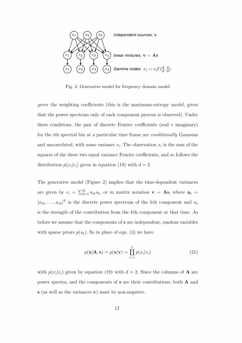
Fig. 2. Generative model for frequency domain model

given the weighting coefficients (this is the maximum-entropy model, given

that the power spectrum only of each component process is observed). Under

these conditions, the pair of discrete Fourier coefficients (real + imaginary)

for the ith spectral bin at a particular time frame are conditionally Gaussian

and uncorrelated, with some variance vi. The observation xi is the sum of the

squares of the these two equal variance Fourier coefficients, and so follows the

distribution p(xi|vi) given in equation (19) with d = 2.

The generative model (Figure 2) implies that the time-dependent variances

are given by vi =∑K

k=1 aiksk, or in matrix notation v = As, where ak =

[a1k, . . . , aIk]T is the discrete power spectrum of the kth component and sk

is the strength of the contribution from the kth component at that time. As

before we assume that the components of s are independent, random variables

with sparse priors p(sk). So in place of eqn. (3) we have

p(x|A, s) = p(x|v) =I∏

i=1

p(xi|vi) (21)

with p(xi|vi) given by equation (19) with d = 2. Since the columns of A are

power spectra, and the components of s are their contributions, both A and

s (as well as the variances v) must be non-negative.

12

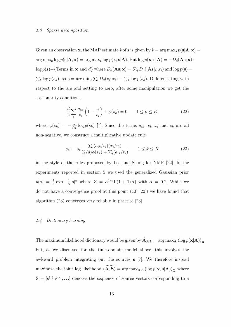
4.3 Sparse decomposition

Given an observation x, the MAP estimate s of s is given by s = arg maxs p(s|A,x) =

arg maxs log p(s|A,x) = arg maxs log p(x, s|A). But log p(x, s|A) = −Dd(As;x)+

log p(s)+{Terms in x and d} where Dd(As;x) =∑

i Dd([As]i; xi) and log p(s) =

∑

k log p(sk), so s = arg mins

∑

i Dd(vi; xi)−∑

k log p(sk). Differentiating with

respect to the sks and setting to zero, after some manipulation we get the

stationarity conditions

d

2

∑

i

aik

vi

(

1− xi

vi

)

+ φ(sk) = 0 1 ≤ k ≤ K (22)

where φ(sk) = − ddsk

log p(sk) [7]. Since the terms aik, vi, xi and sk are all

non-negative, we construct a multiplicative update rule

sk ← sk

∑

i(aik/vi)(xi/vi)

(2/d)φ(sk) +∑

i(aik/vi)1 ≤ k ≤ K (23)

in the style of the rules proposed by Lee and Seung for NMF [22]. In the

experiments reported in section 5 we used the generalized Gaussian prior

p(s) = 1Z

exp− 1α|s|α where Z = α1/αΓ(1 + 1/α) with α = 0.2. While we

do not have a convergence proof at this point (c.f. [22]) we have found that

algorithm (23) converges very reliably in practise [23].

4.4 Dictionary learning

The maximum likelihood dictionary would be given by AML = arg maxA 〈log p(x|A)〉X

but, as we discussed for the time-domain model above, this involves the

awkward problem integrating out the sources s [7]. We therefore instead

maximize the joint log likelihood (A,S) = arg maxA,S 〈log p(x, s|A)〉X

where

S = [s(1), s(2), . . .] denotes the sequence of source vectors corresponding to a

13

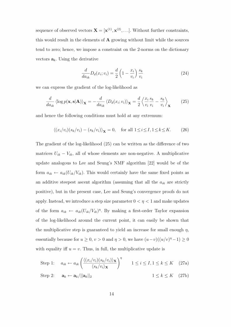
sequence of observed vectors X = [x(1),x(2), . . .]. Without further constraints,

this would result in the elements of A growing without limit while the sources

tend to zero; hence, we impose a constraint on the 2-norms on the dictionary

vectors ak. Using the derivative

d

daik

Dd(xi; vi) =d

2

(

1− xi

vi

)

sk

vi

(24)

we can express the gradient of the log-likelihood as

d

daik

〈log p(x, s|A)〉X

= − d

daik

〈Dd(xi; vi)〉X =d

2

⟨

xi

vi

sk

vi

− sk

vi

⟩

X

(25)

and hence the following conditions must hold at any extremum:

〈(xi/vi)(sk/vi)− (sk/vi)〉X = 0, for all 1≤ i≤I, 1≤k≤K. (26)

The gradient of the log-likelihood (25) can be written as the difference of two

matrices Uik − Vik, all of whose elements are non-negative. A multiplicative

update analogous to Lee and Seung’s NMF algorithm [22] would be of the

form aik ← aik(Uik/Vik). This would certainly have the same fixed points as

an additive steepest ascent algorithm (assuming that all the aik are strictly

positive), but in the present case, Lee and Seung’s convergence proofs do not

apply. Instead, we introduce a step size parameter 0 < η < 1 and make updates

of the form aik ← aik(Uik/Vik)η. By making a first-order Taylor expansion

of the log-likelihood around the current point, it can easily be shown that

the multiplicative step is guaranteed to yield an increase for small enough η,

essentially because for u ≥ 0, v > 0 and η > 0, we have (u−v)((u/v)η−1) ≥ 0

with equality iff u = v. Thus, in full, the multiplicative update is

Step 1: aik ← aik

(

〈(xi/vi)(sk/vi)〉X〈sk/vi〉X

)η

1 ≤ i ≤ I, 1 ≤ k ≤ K (27a)

Step 2: ak ← ak/||ak||2 1 ≤ k ≤ K (27b)

14

where the second step restores unit 2-norm to the columns of A. The s (and

hence v = As) values in (27a) can be computed by, for example, interleaving

the dictionary updates with a few iterations of the decomposition update (23).

5 Experiments

We compared the time-domain and spectral-domain methods by training each

on a recording of Beethoven’s Bagatelle, Opus 33 No. 1 in E♭ Major contain-

ing 57 different played notes. The recording was made using a MIDI-controlled

acoustic piano (i.e. not a synthesized piano) so that an exact MIDI represen-

tation was available alongside the audio recording. The two channels of the

original recording (44.1kHz stereo) were summed to mono, and downsampled

to 8kHz.

The time-domain method used functions of length L = 1024 from a window

of size I = 2L = 2048 samples, with K = 57 functions in the dictionary,

matching the known number of notes played. The dictionary was initialized

to a set of random waveforms. Pitched dictionary vectors were observed to

converge within 24 hours on an Apple PowerMac 1.42GHz dual processor G4,

although the algorithm was run for a total of 7 days to ensure convergence as

much as possible.

The spectral-domain method used a frame size of 1024 samples, giving power

spectra with I = 513 elements, and K = 117 dictionary vectors. The spectral-

domain dictionary was initialized to a 1/2-semitone pitch dictionary plus three

‘spare’ flat initial dictionary vectors. Specifically, the pitched part of the initial

15

dictionary matrix A0 is given by:

a′ij = 1 + 3

(

cos2 (π(fs/fj)(i− 1)/L))ri

(28)

A0 = normaliseA′ (29)

where L is the DFT frame size, fs is the sampling frequency, fj = 440×2mj/12

with mj = −32 + (j − 1)/2 being the pitch of the jth element in semitones

above A4 (440Hz), ri decreases linearly from 3 to 1 as i goes from 1 to N , and

the function normalise(·) rescales each dictionary element to unit 2-norm. The

spectral-domain algorithm was run for 3 hours (120 dictionary updates) on an

Apple PowerBook G4 laptop with single 1.3GHz processor. For comparison,

the NMF method of Smaragdis and Brown [17] was also run from the same

starting conditions as our frequency domain method.

5.1 Dictionary elements

Both our methods, as well as NMF, learned dictionaries that generally reflect

the structure of notes present in the piece. The dictionary waveforms learned

by the time-domain method are shown in Fig. 3. The first 46 atoms had

a clear harmonic structure and are here ordered by increasing fundamental

frequency from bottom to top, while the topmost atoms (47 to 57) could

not be assigned to an individual fundamental frequency. (This ordering was

performed by hand for this example.) Most atoms have full support over their

whole lengths, although some atoms (e.g. 14, 23, 29 and 41) have a shorter

time support.

The spectra of these dictionary waveforms are shown in Fig. 4(a), where this

time the frequency ordering runs from left to right, with the spectra of the

16

12.5 25 37.5 50 62.5 75 87.5 100 112.5 125

123456789

101112131415161718192021222324252627282930313233343536373839404142434445464748495051525354555657

atom

num

ber

time/ms

Fig. 3. Time-domain waveforms of the dictionary learned with the time-domain

method.

(a) (b) (c)

atom number

freq

uenc

y/kH

z

sisc, prior=hyperbolic(2), frame length=1024

10 20 30 40 500

0.5

1

1.5

2

2.5

3

3.5

4

atom number

freq

uenc

y/kH

z

nnsc, prior=genexp2(0.2), frame length=1024

20 40 60 80 1000

0.5

1

1.5

2

2.5

3

3.5

4

atom number

freq

uenc

y/kH

z

nmfdiv, frame length=1024

20 40 60 80 1000

0.5

1

1.5

2

2.5

3

3.5

4

Fig. 4. Spectra of (a) time-domain dictionary waveforms, (b) the dictionary learned

with the spectral-domain approach and (c) the NMF approach.

unordered waveforms on the far right. A clear harmonic structure is visible

from this dictionary. We also notice that some notes are represented by more

than one dictionary element: we shall examine these in more detail later.

The dictionary learned by the spectral-domain method is shown in Fig. 4(b),

with the NMF dictionary spectra in Fig. 4(c). The dictionary atoms for these

also show a harmonic structure, with some notes represented by more than

17

one dictionary element.

We can see that more higher harmonics are visible in the spectral dictionaries

(Fig. 4(b) and (c)) than in the time-domain dictionary spectra (Fig. 4(a)).

This appears to be due to the well-known ‘stretching’ of the upper harmonics

on the piano which in turns means that the upper harmonics will not be phase-

locked to lower harmonics. While this is not an issue for the spectral model

(which ignores phase), it will lead to a continually shifting phase relationship

between the upper and lower harmonics, and hence no single representative

time-domain waveform will be able to represent a sustained note without a

tendency to ‘smear out’ the higher harmonics. We have observed that time-

domain dictionaries trained on other instruments do retain more of the higher

harmonics.

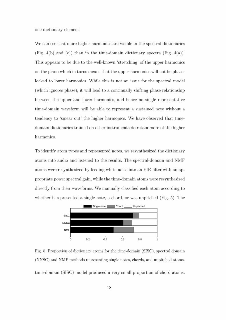
To identify atom types and represented notes, we resynthesized the dictionary

atoms into audio and listened to the results. The spectral-domain and NMF

atoms were resynthesized by feeding white noise into an FIR filter with an ap-

propriate power spectral gain, while the time-domain atoms were resynthesized

directly from their waveforms. We manually classified each atom according to

whether it represented a single note, a chord, or was unpitched (Fig. 5). The

0 0.2 0.4 0.6 0.8 1

SISC

NNSC

NMF

Single note Chord Unpitched

Fig. 5. Proportion of dictionary atoms for the time-domain (SISC), spectral domain

(NNSC) and NMF methods representing single notes, chords, and unpitched atoms.

time-domain (SISC) model produced a very small proportion of chord atoms:

18

this is expected, since it would be unlikely for separate notes in a chord to

maintain the fixed phase relationship required to produce an unchanging wave-

form. Our spectral-domain method (NNSC) produced a higher proportion of

single note atoms compared to the NMF dictionary, suggesting it would be

more appropriate for the automatic music transcription applications we are

interested in.

5.2 Sparse representation

(a) 0 2.5 5 7.5 10 12.5 15 17.5 20 22.5 2513579

11131517192123252729313335373941434547

atom

num

ber

time/s (b) time/s

atom

num

ber

unknown:beet:bag:33, nnsc(genexp2(0.2))

0 5 10 15 20 25

10

20

30

40

50

60

70

80

90

100

110

−15

−10

−5

0

5

10

15

20

25

30

(c) time/s

atom

num

ber

beet:bag:33, nmfdiv

0 5 10 15 20 25

10

20

30

40

50

60

70

80

90

100

110

−15

−10

−5

0

5

10

15

20

25

30

(d) 0 5 10 15 20 25 30 35 40 45C2

F2

A2#

D3#

G3#

C4#

F4#

B4

E5

A5

Time in beats

Pitc

h

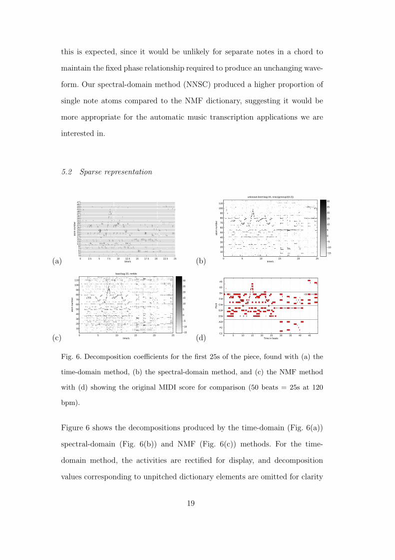
Fig. 6. Decomposition coefficients for the first 25s of the piece, found with (a) the

time-domain method, (b) the spectral-domain method, and (c) the NMF method

with (d) showing the original MIDI score for comparison (50 beats = 25s at 120

bpm).

Figure 6 shows the decompositions produced by the time-domain (Fig. 6(a))

spectral-domain (Fig. 6(b)) and NMF (Fig. 6(c)) methods. For the time-

domain method, the activities are rectified for display, and decomposition

values corresponding to unpitched dictionary elements are omitted for clarity

19

(and in any case do not contribute significantly to the decomposition). All

decomposition methods show melodic lines, chord structures and rhythmic

patterns. However, there are also clear differences: the time-domain represen-

tation is composed of clusters of high-resolution impulses (‘spikes’) to make

up each note, while the frame-based analysis process means that the spectral-

domain and NMF representations are a low-resolution, sustained representa-

tion instead.

Close examination reveals that not all of the notes were successfully recovered:

for example, a few of the lowest MIDI notes are not represented in (Fig. 6(a)).

Also, in all decompositions we can find examples where a particular note is

represented by more than one component. In the spectral-domain represen-

tations (Fig. 6(b) and (c)) this sometimes appears as a ‘comma’ at the start

of each note, as one component is active for the note onset, followed by a

different component for the sustained part of the note.

5.3 Note detection performance

Since both our spectral-domain method (NNSC) and NMF operate on spectral

frames, they admit a direct comparison. Visually, our spectral-domain decom-

position appears ‘cleaner’ than the NMF results, indicating that the sparse

priors have indeed reduced more coefficients to zero in the spectral-domain

method.

For a quantitative comparison between NNSC and NMF we compared the

notes detected by both methods with the original MIDI score in each frame.

We considered two cases: (i) dictionary atoms contribute to any note they

20

contain, and (ii) only dictionary atoms containing a single note contribute to

that note. In each case the activity from atoms contributing to each note are

combined. If the total activity for that note is above a threshold, that note is

considered to be ‘detected’ in that frame. Comparison with the original MIDI

score (Fig. 6(d)) at a range of thresholds, yielded the performance curves

shown in Fig. 7. As expected, including ‘chord’ dictionary atoms increases good

0 0.2 0.4 0.6 0.8 10

0.1

0.2

0.3

0.4

0.5

0.6

0.7

0.8

0.9

1

false positives

true

pos

itive

s

nnsc(genexp2(0.2)):bmap(filternp)nnsc(genexp2(0.2)):bmap(filterchords)nmfdiv:bmap(filternp)nmfdiv:bmap(filterchords)

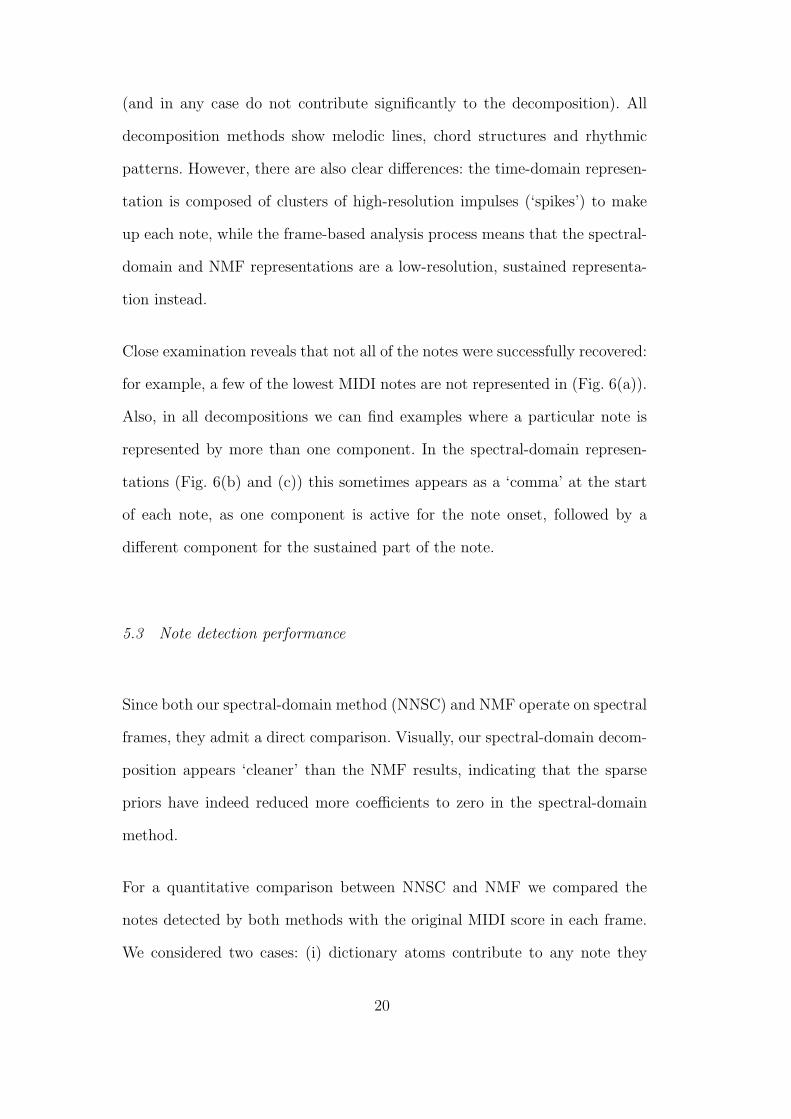
Fig. 7. Note detection performance of spectral domain (NNSC) method and NMF

method over a range of thresholds. Binary maps of notes detected are compared

with current ‘on’ MIDI notes on a frame by frame basis. For the curves ‘filternp’

dictionary atoms contribute to each note they contain, while unpitched dictionary

atoms are filtered out. Each note detector at each frame is classified as true-posi-

tive (TP), false-positive (FP), true-negative (TN) or false-negative (FN). The ‘true

positive’ (Good detection, recall) coefficient is TP/(TP+FN), where TP+FN is the

total number of ‘on’ pixels in the map of the original ‘true’ MIDI score. The ‘false

positive’ (1 − precision) coefficient is FP/(TP+FP), where TP+FP is the total

number of ‘on’ pixels in the map of the detected notes. For the curves ‘filterchords’

only dictionary atoms that contain a single note are included: the chord atoms are

filtered out (as well as the unpitched atoms).

detections slightly at the cost of slightly increased false positives. However, we

21

can clearly see that our spectral-domain (NNSC) method produces a better

trade-off of performance across the range of thresholds than the NMF method.

5.4 Representation of notes by multiple components

As we mentioned earlier, the representations found by these methods contain

some sets of components that together represented a single note: these tended

to correspond to the notes that appeared most often in the recording. We call

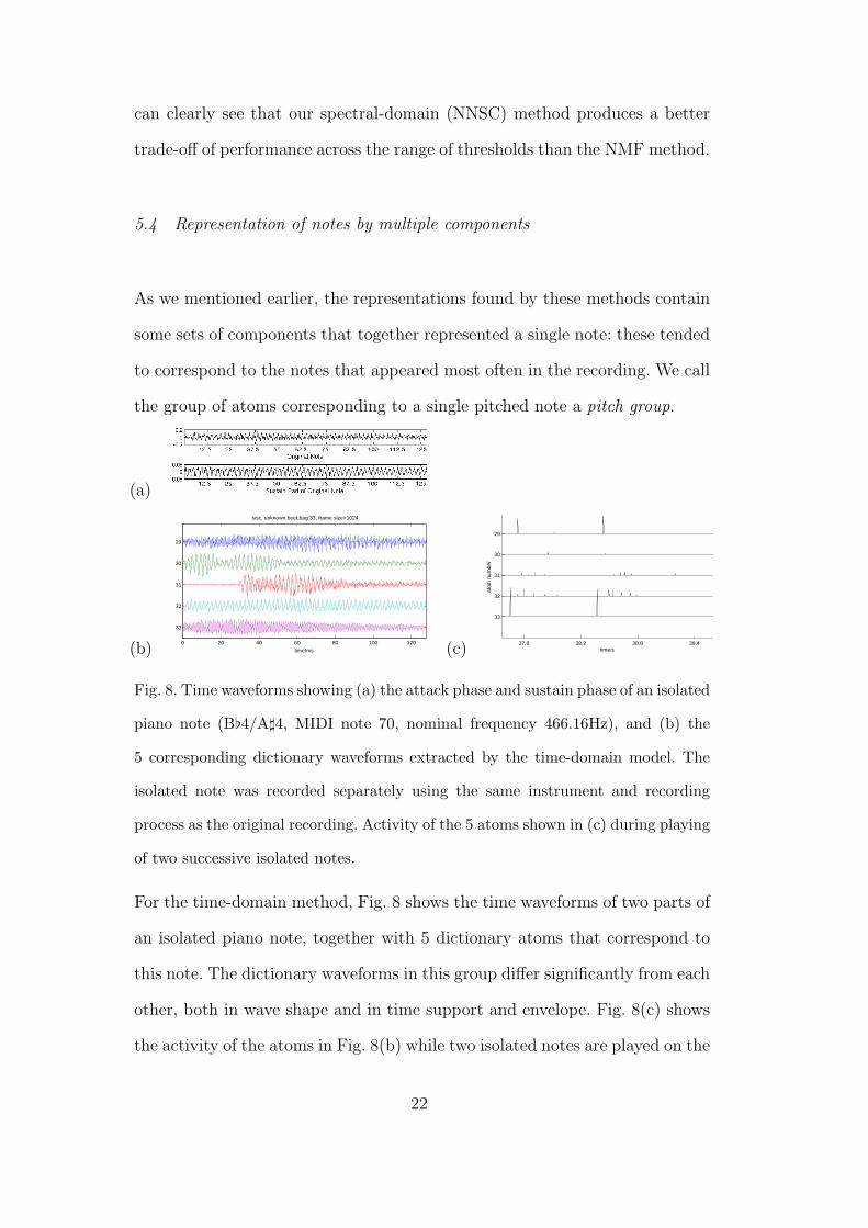
the group of atoms corresponding to a single pitched note a pitch group.

(a)

(b)0 20 40 60 80 100 120

33

32

31

30

29

time/ms

sisc, unknown:beet:bag:33, frame size=1024

(c)37.6 38.2 38.8 39.4

33

32

31

30

29

atom

num

ber

time/s

Fig. 8. Time waveforms showing (a) the attack phase and sustain phase of an isolated

piano note (B♭4/A♯4, MIDI note 70, nominal frequency 466.16Hz), and (b) the

5 corresponding dictionary waveforms extracted by the time-domain model. The

isolated note was recorded separately using the same instrument and recording

process as the original recording. Activity of the 5 atoms shown in (c) during playing

of two successive isolated notes.

For the time-domain method, Fig. 8 shows the time waveforms of two parts of

an isolated piano note, together with 5 dictionary atoms that correspond to

this note. The dictionary waveforms in this group differ significantly from each

other, both in wave shape and in time support and envelope. Fig. 8(c) shows

the activity of the atoms in Fig. 8(b) while two isolated notes are played on the

22

recorded piano. This clearly shows that atoms 33 and 29 are used to represent

the note onset, atom 30 is used only once in each note, while the other two

atoms (31, 32) are used repeatedly with varying magnitude to represent the

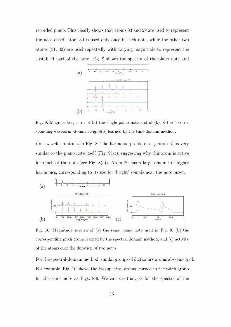
sustained part of the note. Fig. 9 shows the spectra of the piano note and

(a)

(b) 0 0.5 1 1.5 2 2.5 3 3.5 4

33

32

31

30

29

frequency/kHz

sisc, unknown:beet:bag:33, frame size=1024

Fig. 9. Magnitude spectra of (a) the single piano note and of (b) of the 5 corre-

sponding waveform atoms in Fig. 8(b) learned by the time-domain method.

time waveform atoms in Fig. 8. The harmonic profile of e.g. atom 31 is very

similar to the piano note itself (Fig. 9(a)), suggesting why this atom is active

for much of the note (see Fig. 8(c)). Atom 29 has a large amount of higher

harmonics, corresponding to its use for ‘bright’ sounds near the note onset.

(a)

(b)0 500 1000 1500 2000 2500 3000 3500 4000

79

80

atom

num

ber

frequency/Hz

Pitch class: #a/4

(c)10 10.5 11 11.5 12

79

80

atom

num

ber

times/s

Pitch class: #a/4

Fig. 10. Magnitude spectra of (a) the same piano note used in Fig. 9, (b) the

corresponding pitch group learned by the spectral domain method, and (c) activity

of the atoms over the duration of two notes.

For the spectral-domain method, similar groups of dictionary atoms also emerged.

For example, Fig. 10 shows the two spectral atoms learned in the pitch group

for the same note as Figs. 8-9. We can see that, as for the spectra of the

23

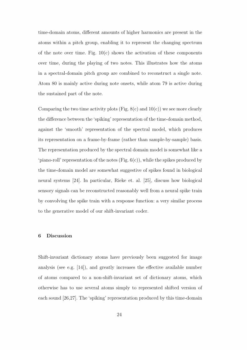
time-domain atoms, different amounts of higher harmonics are present in the

atoms within a pitch group, enabling it to represent the changing spectrum

of the note over time. Fig. 10(c) shows the activation of these components

over time, during the playing of two notes. This illustrates how the atoms

in a spectral-domain pitch group are combined to reconstruct a single note.

Atom 80 is mainly active during note onsets, while atom 79 is active during

the sustained part of the note.

Comparing the two time activity plots (Fig. 8(c) and 10(c)) we see more clearly

the difference between the ‘spiking’ representation of the time-domain method,

against the ‘smooth’ representation of the spectral model, which produces

its representation on a frame-by-frame (rather than sample-by-sample) basis.

The representation produced by the spectral domain model is somewhat like a

‘piano-roll’ representation of the notes (Fig. 6(c)), while the spikes produced by

the time-domain model are somewhat suggestive of spikes found in biological

neural systems [24]. In particular, Rieke et. al. [25], discuss how biological

sensory signals can be reconstructed reasonably well from a neural spike train

by convolving the spike train with a response function: a very similar process

to the generative model of our shift-invariant coder.

6 Discussion

Shift-invariant dictionary atoms have previously been suggested for image

analysis (see e.g. [14]), and greatly increases the effective available number

of atoms compared to a non-shift-invariant set of dictionary atoms, which

otherwise has to use several atoms simply to represented shifted version of

each sound [26,27]. The ‘spiking’ representation produced by this time-domain

24

method indicates that this might lead us towards an “event-based” representa-

tion of musical audio. In such a representation, we would be able to represent

a sound by a time index and object description (or a composition of a few of

these) to producing a representation in terms of “sound objects” [28].

On the other hand, the spectral domain approach to polyphonic music analy-

sis, modelling observed spectra as a linear sum of weighted note spectra, has

attracted a significant amount of interest from the blind source separation

community recently. As well as our own work using independent component

analysis (ICA) [15,19], non-negative ICA [18], and sparse coding [19,20,29],

independent subspace analysis (ISA) has been used by Casey and Westner

[16], non-negative matrix factorization (NMF) by Smaragdis and Brown [17]

and non-negative sparse coding (NNSC) combined with a discontinuity cost

by Virtanen [30].

The spectral domain method described here differs from these earlier ap-

proaches in that we do not simply assume linear addition of spectra with the

usual squared error, but derive a non-negative sparse coding model through

a model of estimation of variance using a gamma distribution, which leads

to multiplicative noise [23]. While we therefore have a “non-negative sparse

coder”, in this sense our approach is perhaps closer to the nonlinear ISA gener-

ative model approach of Vincent and Rodet [31], although our approach differs

from Hoyer’s [21] non-negative sparse coding method. Gamma distributions

have also been suggested for separation of positive sources by Moussaoui et.

al. [32].

We note that NMF alone has recently been shown to reliably give a parts-based

decomposition under certain circumstances [33], and it would be interesting to

25

consider whether there are similar proofs for the type of non-negative sparse

coder considered here. We are also currently investigating the use of shift-

invariant strategy in the spectral domain to get shift-invariant non-negative

sparse coding in a dictionary of time-frequency atoms, related to the methods

suggested by Smaragdis [34] and Virtanen [35], with encouraging initial results.

For our experiments we used a MIDI-controlled acoustic piano so that an exact

MIDI representation was available corresponding to a realistic musical audio

performance including appropriate dynamics. Nevertheless, we might expect

transcription from a live human player to be somewhat more challenging, due

to the additional variability in the performance that could not be captured

in the MIDI data stream. Furthermore, other instruments, such as stringed

instruments, have additional scope for expressive playing (e.g. vibrato in string

instruments): we expect that these will require more complex generative mod-

els [31].

7 Conclusions

We have developed two approaches for sparse decomposition of polyphonic

music: a time-domain approach based on shift-invariant waveforms, and a

frequency-domain approach based on phase-invariant power spectra, and we

have shown that both methods can successfully produce a sparse represen-

tation from a MIDI-controlled acoustic piano recording. We also compared

our frequency-domain method against the non-negative matrix factorization

(NMF) frequency-domain approach of Smaragdis and Brown [17].

Comparing the dictionaries, we found that the time-domain atoms lose some

26

of the higher harmonics of piano notes, perhaps due to ‘stretching’ of upper

harmonics on the piano. However, the time-domain dictionary does produce a

higher proportion of single-note atoms than the frequency-domain algorithms.

Our frequency-domain sparse coding algorithm yields a dictionary with more

single-note atoms than the NMF dictionary.

The time-domain method produces a sparse activity representation consisting

of ‘spikes’ making up the sequence notes, somewhat reminiscent of biologi-

cal neural activity. On the other hand, the frequency-domain methods (both

our non-negative sparse coding and NMF) produce a ‘piano-roll’ representa-

tion that can be compared directly to on/off activity in the original MIDI

data. Comparing frame-by-frame note detection performance, we found our

frequency-domain method clearly outperformed NMF on this recording, re-

gardless of whether chord atoms were included or not. Nevertheless, NMF has

been reported to perform well on other tasks, and it would be interesting to

systematically compare these various algorithms on a wide range of musical

audio recordings.

Of our two sparse coding methods, each has its own advantages and disad-

vantages. The time-domain method is computationally expensive (even when

our subspace selection approximation is used), but produces sample-accurate

spike-like activations. These suggest possible future application of this ap-

proach in event-based representations, and could be used for a direct time-

domain reconstruction. The spectral domain method discards phase informa-

tion, which would need to be restored for signal reconstruction [36], but is

faster than the time-domain method. The piano spectral dictionary for the

frequency-domain method contains more higher harmonics despite the lack of

phase-locking of these higher harmonics.

27

These techniques already indicate that sparse coding is a powerful approach

to automatic music transcription or object-based coding of musical audio. It

would be interesting to see if these techniques can be combined, for example

through initial learning of spectra leading to derived waveforms, to combine

the best of the two methods.

Acknowledgements

This work was partially supported by Grants GR/R54620/01, GR/S75802/01,

GR/S84743/01 and GR/S82213/01 from the UK Engineering and Physical

Sciences Research Council, and by EU-FP6-IST-507142 project SIMAC (Se-

mantic Interaction with Music Audio Contents). The authors would also like

to thank two anonymous referees, whose comments helped to significantly

improve this paper.

References

[1] J. C. Brown, B. Zhang, Musical frequency tracking using the methods of

conventional and narrowed autocorrelation, Journal of the Acoustical Society

of America 89 (5) (1991) 2346–2354.

[2] K. D. Martin, A blackboard system for automatic transcription of simple

polyphonic music, Tech. Rep. 385, MIT Media Lab, Perceptual Computing

Section (July 1996).

[3] K. Kashino, K. Nakadai, T. Kinoshita, H. Tanaka, Application of Bayesian

probability network to music scene analysis, in: Working Notes of the IJCAI-95

Computational Auditory Scene Analysis Workshop, 1995, pp. 52–59.

28

[4] A. Klapuri, T. Virtanen, J.-M. Holm, Robust multipitch estimation for the

analysis and manipulation of polyphonic musical signals, in: Proc. COST-G6

Conference on Digital Audio Effects, DAFx-00, Verona, Italy, 2000, pp. 141–146.

[5] M. Marolt, Networks of adaptive oscillators for partial tracking and

transcription of music recordings, Journal of New Music Research 33 (1) (2004)

49–59.

[6] B. A. Olshausen, D. J. Field, Emergence of simple-cell receptive-field properties

by learning a sparse code for natural images, Nature 381 (1996) 607–609.

[7] K. Kreutz-Delgado, J. F. Murray, B. D. Rao, K. Engan, T.-W. Lee, T. J.

Sejnowski, Dictionary learning algorithms for sparse representation, Neural

Computation 15 (2003) 349–396.

[8] T. Blumensath, M. E. Davies, Unsupervised learning of sparse and shift-

invariant decompositions of polyphonic music, in: Proc. IEEE International

Conference on Acoustics, Speech, and Signal Processing (ICASSP ’04), Vol. 5,

2004, pp. V:497–V:500.

[9] T. Blumensath, M. E. Davies, On shift-invariant sparse coding, in: C. G.

Puntonet, A. Prieto (Eds.), Independent Component Analysis and Blind Signal

Separation: Proc. Fifth Intl. Conf., ICA 2004, Granada, Spain, Springer, Berlin,

2004, pp. 1205–1212, LNCS 3195.

[10] S. S. Chen, D. L. Donoho, M. A. Saunders, Atomic decomposition by basis

pursuit, SIAM Journal on Scientific Computing 20 (1) (1998) 33–61.

[11] M. A. T. Figueiredo, A. K. Jain, Bayesian learning of sparse classifiers, in: Proc.

2001 IEEE Computer Society Conference on Computer Vision and Pattern

Recognition (CVPR 2001), Vol. 1, 2001, pp. I–35 – I–41.

[12] J. A. Nelder, R. W. M. Wedderburn, Generalized linear models, Journal of the

Royal Statistical Society, Series A (General) 135 (3) (1972) 370–384.

29

[13] J. F. Murray, K. Kreutz-Delgado, An improved FOCUSS-based learning

algorithm for solving sparse linear inverse problems, in: Conference Record

of the Thirty-Fifth Asilomar Conference on Signals, Systems and Computers,

2001, pp. 347–351.

[14] P. Sallee, B. A. Olshausen, Learning sparse multiscale image representations,

in: S. Becker, S. Thrun, K. Obermayer (Eds.), Advances in Neural Information

Processing Systems, 15, MIT Press, 2003, pp. 1327–1334.

[15] M. D. Plumbley, S. A. Abdallah, J. P. Bello, M. E. Davies, G. Monti,

M. B. Sandler, Automatic music transcription and audio source separation,

Cybernetics and Systems 33 (6) (2002) 603–627.

[16] M. Casey, A. Westner, Separation of mixed audio sources by independent

subspace analysis, in: Proc. International Computer Music Conference (ICMC

2000), Berlin, 2000.

[17] P. Smaragdis, J. Brown, Non-negative matrix factorization for polyphonic

music transcription, in: Proc. 2003 IEEE Workshop on Applications of Signal

Processing to Audio and Acoustics, New Paltz, New York, 2003, pp. 177–180.

[18] M. D. Plumbley, Algorithms for nonnegative independent component analysis,

IEEE Transactions on Neural Networks 14 (3) (2003) 534–543.

[19] S. A. Abdallah, Towards music perception by redundancy reduction and

unsupervised learning in probabilistic models, Ph.D. thesis, Department of

Electronic Engineering, King’s College London, UK (2002).

[20] S. A. Abdallah, M. D. Plumbley, An independent component analysis approach

to automatic music transcription, in: Proc. 114th Convention of the Audio

Engineering Society, Amsterdam, The Netherlands, 2003.

[21] P. O. Hoyer, Non-negative sparse coding, in: Neural Networks for Signal

Processing XII (Proc. IEEE Workshop on Neural Networks for Signal

30

Processing), Martigny, Switzerland, 2002, pp. 557–565.

[22] D. D. Lee, H. S. Seung, Algorithms for non-negative matrix factorization, in:

T. K. Leen, T. G. Dietterich, V. Tresp (Eds.), Advances in Neural Information

Processing Systems 13, MIT Press, 2001, pp. 556–562.

[23] S. A. Abdallah, M. D. Plumbley, Polyphonic transcription by non-negative

sparse coding of power spectra, in: Proc. 5th Int. Conf. on Music Information

Retrieval (ISMIR 2004), Barcelona, Spain, 2004, pp. 318–325.

[24] B. A. Olshausen, Sparse codes and spikes, in: R. P. N. Rao, B. A. Olshausen,

M. S. Lewicki (Eds.), Probabilistic Models of the Brain: Perception and Neural

Function, MIT Press, 2002, pp. 257–272.

[25] F. Rieke, D. Warland, R. R. de Ruyter Van Steveninck, W. Bialek, Spikes:

Exploring the Neural Code, MIT Press, Cambridge, MA, 1997.

[26] A. J. Bell, T. J. Sejnowski, Learning the higher-order structure of a natural

sound, Network: Computation in Neural Systems 7 (1996) 261–267.

[27] S. A. Abdallah, M. D. Plumbley, If edges are the independent components of

natural images, what are the independent components of natural sounds?, in:

T.-W. Lee, T.-P. Jung, S. Makeig, T. J. Sejnowski (Eds.), Proc. International

Conference on Independent Component Analysis and Blind Signal Separation

(ICA2001), San Diego, California, 2001, pp. 534–539.

[28] X. Amatriain, P. Herrera, Transmitting audio content as sound objects, in: Proc.

AES 22nd International Conference on Virtual, Synthetic and Entertainment

Audio, Espoo, Finland, 2002.

[29] S. A. Abdallah, M. D. Plumbley, Unsupervised analysis of polyphonic

music using sparse coding in a probabilistic framework, To appear in IEEE

Transactions on Neural Networks.

31

[30] T. Virtanen, Sound source separation using sparse coding with temporal

continuity objective, in: H. C. Kong, B. T. G. Tan (Eds.), Proc. International

Computer Music Conference (ICMC 2003), Singapore, 2003, pp. 231–234.

[31] E. Vincent, X. Rodet, Music transcription with ISA and HMM, in: C. G.

Puntonet, A. Prieto (Eds.), Independent Component Analysis and Blind Signal

Separation: Proc. Fifth International Conference, ICA 2004, Granada, Spain,

Springer, Berlin, 2004, pp. 1197–1204, LNCS 3195.

[32] S. Moussaoui, D. Brie, O. Caspary, A. Mohammad-Djafari, A Bayesian method

for positive source separation, in: Proc. IEEE International Conference on

Acoustics, Speech, and Signal Processing (ICASSP ’04), Vol. 5, 2004, pp. V–

485–V–488.

[33] D. Donoho, V. Stodden, When does non-negative matrix factorization give a

correct decomposition into parts?, in: S. Thrun, L. Saul, B. Scholkopf (Eds.),

Advances in Neural Information Processing Systems 16, MIT Press, Cambridge,

MA, 2004.

[34] P. Smaragdis, Non-negative matrix factor deconvolution: Extraction of multiple

sound sources from monophonic inputs, in: Independent Component Analysis

and Blind Signal Separation: Proc. Fifth International Conference (ICA 2004),

Granada, Spain, 2004, pp. 494–499.

[35] T. Virtanen, Separation of sound sources by convolutive sparse coding, in: Proc.

ISCA Workshop on Statistical and Perceptual Audio Processing (SAPA 2004),

Jeju, Korea, 2004.

[36] K. Achan, S. T. Roweis, B. J. Frey, Probabilistic inference of speech signals from

phaseless spectrograms, in: S. Thrun, L. Saul, B. Scholkopf (Eds.), Advances in

Neural Information Processing Systems 16, MIT Press, Cambridge, MA, 2004,

pp. 1393–1400.

32