Embed Size (px)
Citation preview

Sparse modeling of risk factors in insurance analytics
Sander Devriendt
Joint work with Katrien Antonio, Edward Frees and Roel Verbelen
R in Insurance ConferenceParis, June 8, 2017
Sparse modeling of risk factors in insurance analytics 1/23

Outline
1 Motivation: insurance pricing
2 Regularization, penalties and the LASSO
3 A unified framework
4 Conclusion and further research
Sparse modeling of risk factors in insurance analytics 2/23

Motivation: actuarial models in insurance pricing
Problem: determine the (pure) premium πi for insured i with
number of claims Ni over exposure ei,
aggregate loss Li over exposure ei.
Decompose the premium in frequency and severity:
πi = E
[Li
ei
]= E
[Ni
ei
]× E
[Li
Ni
]= E [Freqi]× E [Sevi] .
Classical assumption of independence allows for separate predictive modelingof E [Freqi] and E [Sevi].
Sparse modeling of risk factors in insurance analytics 3/23
Motivation: actuarial models in practice
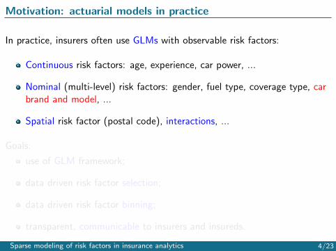
In practice, insurers often use GLMs with observable risk factors:
Continuous risk factors: age, experience, car power, ...
Nominal (multi-level) risk factors: gender, fuel type, coverage type, carbrand and model, ...
Spatial risk factor (postal code), interactions, ...
Goals:
use of GLM framework;
data driven risk factor selection;
data driven risk factor binning;
transparent, communicable to insurers and insureds.
Sparse modeling of risk factors in insurance analytics 4/23

Motivation: actuarial models in practice
In practice, insurers often use GLMs with observable risk factors:
Continuous risk factors: age, experience, car power, ...
Nominal (multi-level) risk factors: gender, fuel type, coverage type, carbrand and model, ...
Spatial risk factor (postal code), interactions, ...
Goals:
use of GLM framework;
data driven risk factor selection;
data driven risk factor binning;
transparent, communicable to insurers and insureds.
Sparse modeling of risk factors in insurance analytics 4/23
Motivation: beyond current practice
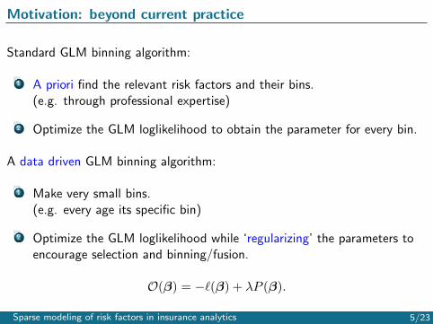
Standard GLM binning algorithm:
1 A priori find the relevant risk factors and their bins.(e.g. through professional expertise)
2 Optimize the GLM loglikelihood to obtain the parameter for every bin.
A data driven GLM binning algorithm:
1 Make very small bins.(e.g. every age its specific bin)
2 Optimize the GLM loglikelihood while ‘regularizing’ the parameters toencourage selection and binning/fusion.
O(β) = −`(β) + λP (β).
Sparse modeling of risk factors in insurance analytics 5/23

Regularization: the LASSO
2D exampleO(β) = −`(β) + λ (|β1|+ |β2|) .
Constraint is sharp,non-smooth.
Encourages selection ofeither β1 or β2.
Extensively studied andefficiently solved.
‘The Elements of Statistical Learning’Hastie et al. (2009).
Sparse modeling of risk factors in insurance analytics 6/23

LASSO regularization
0 5 10 15
−0.
2−
0.1
0.0
0.1
0.2
λ
Coo
rdin
ates
of β
Sparse modeling of risk factors in insurance analytics 7/23

Beyond the LASSO
LASSO has been extensively studied and used (but largely unexplored inactuarial literature).
DNA - gene selection (classical example).
Portfolio selection: select the most important stocks for a certainstrategy.
LASSO regularization is not fit for all types of variables, but can be adjustedto the type of risk factor. E.g. ‘age’, ‘bm-scale’?
1 Determine the type of your risk factor.
2 Allocate a logical penalty to your risk factor.
Sparse modeling of risk factors in insurance analytics 8/23

Matching regularization to type of risk factor
Ordinal risk factors (e.g. age): Fused Lasso
λ∑i
wi|βi+1 − βi|.
Nominal risk factors (e.g. car brand and model): Generalized FusedLasso
λ∑i>k
wi,k|βi − βk|.
Spatial risk factors (e.g. postal code): Graph Guided Fused Lasso
λ∑
(i,k)∈G
wi,k|βi − βk|.
. . .
Sparse modeling of risk factors in insurance analytics 9/23

Fused Lasso
0 2 4 6 8 10 12
−0.
10−
0.05
0.00
0.05
0.10
0.15
λ
Coo
rdin
ates
of β
Sparse modeling of risk factors in insurance analytics 10/23

Generalized Fused Lasso
0.0 0.5 1.0 1.5 2.0
−0.
10−
0.05
0.00
0.05
0.10
0.15
λ
Coo
rdin
ates
of β
Sparse modeling of risk factors in insurance analytics 11/23

Interludium
Regularization is very popular in machine learning (big data!) andstatistics literature BUT only does regularization with one type of riskfactor at a time.
Efficient algorithms and R packages are available in the Gaussian caseand for ‘one type/penalty’
glmnet (Simon): Lasso, ridge en elastic net for GLMs.
genlasso (Arnold): 1D and 2D Fused Lasso, signal approximation, trendfiltering for Gaussian case.
Need for:
Extension of literature and algorithms to GLMs.
Simultaneously work with risk factors of different types.
Sparse modeling of risk factors in insurance analytics 12/23

A unified framework??
Gertheiss - Tutz - Oelker (2010-2016)‘Sparse modeling of categorial explanatory variables’ - Annals of AppliedStatistics
GLM implementation.
Many different penalties.
R package available: gvcm.cat (not maintained).
But...Fitting algorithm: ‘local quadratic approximation’ and subsequent quadraticprogramming:
Only approximate clustering.
How to choose approximation accuracy? Cluster accuracy?
Computationally intensive.
Sparse modeling of risk factors in insurance analytics 13/23

Local quadratic approximation
−1.0 −0.5 0.0 0.5 1.0
0.0
0.2
0.4
0.6
0.8
1.0
x
|x|
|x|lqa
Sparse modeling of risk factors in insurance analytics 14/23
A unified framework!!
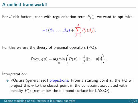
For J risk factors, each with regularization term Pj(), we want to optimize:
−` (β1, . . . ,βJ) +
J∑j=1
Pj (βj),
For this we use the theory of proximal operators (PO):
ProxP (v) = argminz
(P (z) +
1
2||z − v||22
).
Interpretation:
POs are (generalized) projections. From a starting point v, the PO willproject this v to the closest point in the constraint associated withpenalty P () (remember the diamond surface for LASSO).
Sparse modeling of risk factors in insurance analytics 15/23
Optimization algorithm using proximal operators
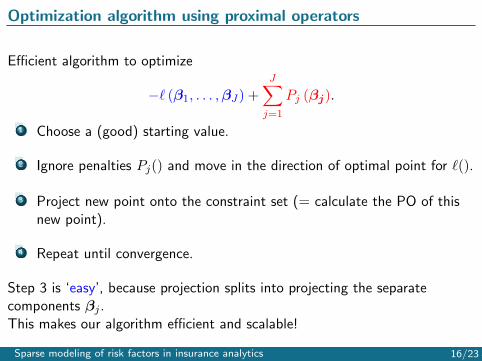
Efficient algorithm to optimize
−` (β1, . . . ,βJ) +
J∑j=1
Pj (βj).
1 Choose a (good) starting value.
2 Ignore penalties Pj() and move in the direction of optimal point for `().
3 Project new point onto the constraint set (= calculate the PO of thisnew point).
4 Repeat until convergence.
Step 3 is ‘easy’, because projection splits into projecting the separatecomponents βj .This makes our algorithm efficient and scalable!
Sparse modeling of risk factors in insurance analytics 16/23
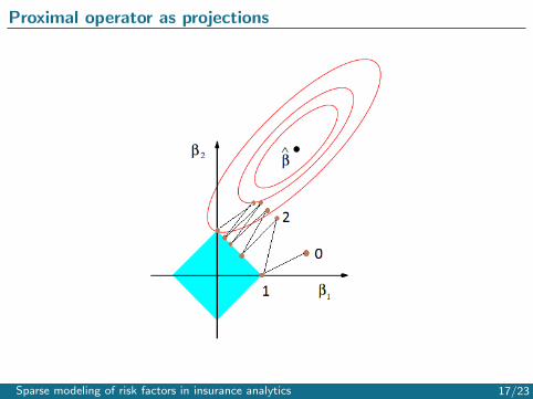
Proximal operator as projections
Sparse modeling of risk factors in insurance analytics 17/23
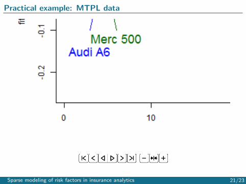
Practical example: MTPL data
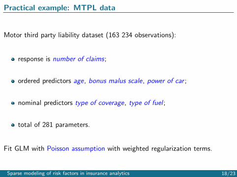
Motor third party liability dataset (163 234 observations):
response is number of claims;
ordered predictors age, bonus malus scale, power of car ;
nominal predictors type of coverage, type of fuel ;
total of 281 parameters.
Fit GLM with Poisson assumption with weighted regularization terms.
Sparse modeling of risk factors in insurance analytics 18/23
Practical example: MTPL data
50 100 150 200 250
−1.
0−
0.5
0.0
0.5
1.0
1.5
2.0
power: Best BIC model
power level
para
met
er v
alue
gam fitpenalization best BICpenalization refit
lambda = 6326.83
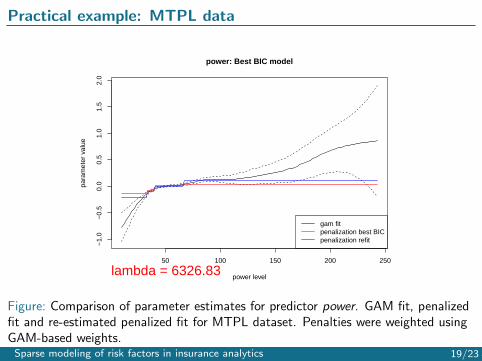
Figure: Comparison of parameter estimates for predictor power. GAM fit, penalizedfit and re-estimated penalized fit for MTPL dataset. Penalties were weighted usingGAM-based weights.Sparse modeling of risk factors in insurance analytics 19/23
Practical example: MTPL data
20 40 60 80
−0.
20.
00.
20.
4
age: Best BIC model
age level
para
met
er v
alue
gam fitpenalization best BICpenalization refit
lambda = 6326.83
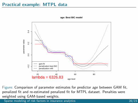
Figure: Comparison of parameter estimates for predictor age between GAM fit,penalized fit and re-estimated penalized fit for MTPL dataset. Penalties wereweighted using GAM-based weights.Sparse modeling of risk factors in insurance analytics 20/23
Practical example: MTPL data
Sparse modeling of risk factors in insurance analytics 21/23
Conclusion: our contribution
Applying machine learning techniques to a classical statistical problem.
Implementing an efficient algorithm which is scalable and interpretable.
Flexibility of regularization takes into account type/structure of riskfactor.
Works for all popular penalties.
Makes use of available penalty-specific literature.
Sparse modeling of risk factors in insurance analytics 22/23

Conclusion: further research
Further improving algorithm efficiency.
Implementing new penalties for spatial information, interaction effects...
R package building in progress.
Write a paper!
Sparse modeling of risk factors in insurance analytics 23/23
References I
[1] R. Tibshirani (1996)Regression shrinkage and selection via the lasso.Journal of the Royal Statistical Society, Series B, vol. 58, no. 1, pp.267-288.
[2] R. Tibshirani, M. Saunders, J. Zhu, K. Knight (2005)Sparsity and smoothness via the fused lasso.Journal of the Royal Statistical Society, Series B, vol. 67, no. 1, pp.91-108.
[3] J. Lee, B. Recht, R. Salakhutdinov, N. Srebro, J. Tropp (2010),Practical largescale optimization for max-norm regularization.Advances in Neural Information Processing Systems, vol. 23, pp.1297-1305.
Sparse modeling of risk factors in insurance analytics 24/23

References II
[4] K. Toh, S. Yun (2010),An accelerated proximal gradient algorithm for nuclear norm regularizedleast squares problems.Pacific Journal of Optimization, vol. 6, pp. 615-640.
[5] J. Gertheiss, G. Tutz (2010)Sparse modeling of categorial explanatory variables.The Annals of Applied Statistics, vol. 4, no. 4, pp. 2150-2180.
[6] N. Parikh, S. Boyd, (2014),Proximal Algorithms.Foundations and Trends in Optimization, 1(3), pp. 123-231.
Sparse modeling of risk factors in insurance analytics 25/23

References III
[7] T. Arnold, R. Tibshirani (2016),Efficient Implementations of the Generalized Lasso Dual Path Algorithm.Journal of Computational and Graphical Statistics, vol. 25, no.1 pp. 1-27.
[8] Y. Nesterov (2007),Gradient methods for minimizing composite objective function.CORE Discussion paper, Catholic University of Louvain, 2007/76.
Sparse modeling of risk factors in insurance analytics 26/23