Sparse Graphs (from noisy data, obviously)Sparse Graphs (from noisy data, obviously) Ernst Wit Johann Bernoulli Institute University of Groningen October 4, 2012 Ernst Wit Sparse graphs

Sparse Graphs(from noisy data, obviously)

Ernst Wit

Johann Bernoulli InstituteUniversity of Groningen

October 4, 2012

Ernst Wit Sparse graphs

God is the answer. But what was the question?

A common design: Many (possibly: redundant) items are (sometimes:automatically) screened (possibly: through time).

Possible question

Can we find a sparse dependency structure among the items, possibly withlongitudinal structure.


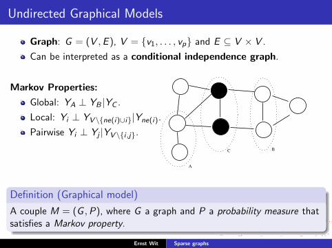
Undirected Graphical Models

Graph: G = (V ,E ), V = {v1, . . . , vp} and E ⊆ V × V .

Can be interpreted as a conditional independence graph.

Markov Properties:

Global: YA ⊥ YB |YC .

Local: Yi ⊥ YV \{ne(i)∪i}|Yne(i).

Pairwise Yi ⊥ Yj |YV \{i ,j}.

A

C B

Definition (Graphical model)

A couple M = (G ,P), where G a graph and P a probability measure thatsatisfies a Markov property.


Factorization and Markov properties

Theorem (Hammersley-Clifford)

If the density p=dP is positive and continuous then

Factorization⇐⇒ Markov(Global/Local/Pairwise)

Factorization: f (y) = 1z

∏c∈C hc(yc), where c are cliques of G .

c1

c2

c3

c4

c5

c6

Example:Graph (left) contains6 cliques (completesubgraphs), and so

p(y) =6∏

i=1

hi (yci ).


Gaussian graphical models

Definition (Gaussian graphical model)

GGM is a graphical model (G ,P), where P is determined by:

Y ∼ N(µ,Θ−1).

Note:

p(y) ∝ exp

(−1

2(y − µ)′Θ(y − µ)

)=

p∏i=1

p∏j=1

e−(yi−µi )(yj−µj )θij/2

=∏c∈C

hc(yc)

So, if θij = 0, then certainly nodes i and j are not in same clique:

θij = 0⇔ Yi ⊥ Yj |YV \{i ,j}.


Traditional: Hypothesis Test

H0 : θij = 0 ⇐⇒ Edge (i , j) is absent

H1 : θij 6= 0 ⇐⇒ Edge (i , j) is present

Dev , 2(l(Θ̂)− argmaxΘ∈H0l(Θ)).

argmaxΘl(Θ)

The space of values for Θ

The space H0

b

bDev

H1

Under H0 and regularity conditions Dev ∼ χ21

p − value = Pr(χ21 ≥ observed deviance)

H0 is rejeced if p-value < 0.05


Problems with Hypothesis Test

Hypothesis tests have poor model selection properties.

Where do we start to test?

Multiple testing problem.

Space of models is of size 2(p2).

If p > n, then S is singular.


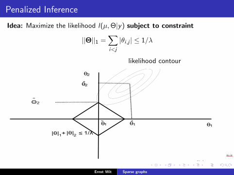
Penalized Inference

Idea: Maximize the likelihood l(µ,Θ|y) subject to constraint

||Θ||1 =∑i<j

|θi ,j | ≤ 1/λ

likelihood contour

θ1

θ2

|θ|1+|θ|2 ≤ 1/λ

θ̂1

θ̂2

Θ̃ 2

θ1˜


Motivation: Dynamic Genomic Networks

Transcription: snap-shot of gene activity in time and space (tissue).

High-throughput microarray and RNA-seq data measure gene activity.

Running example: T-cell time-series dataset.

Temporal expression of 58 genes for 10 unequally spaced time points.

At each time point there are 44 separate measurements.

Definition (Aim)

Determine dynamic genomic graph G on basis of {Y (i)gt }gti .


Motivation: Features of a Dynamic Genomic Process

“p >> n”:I Number of observations smaller than number of variables.I Thousands of variables and hundreds of observations.

Structure:I Highly complex and structured phenomenon.I Possibly with additional topographical structure (small world).

Sparsity: only small number of links between nodes.


Dynamic Genomic Graphs

Γ be a set of “genes”.

T be a set of ordered “time points”.

Definition (Dynamic genomic graph)

A dynamic genomic graph is a pair G = (V ,E ).

Vertices: V = {vij}i∈Γ,j∈T , where Γ and T are finite sets.

Links: ordered pair of elements E ⊆ V × V .

Time1

Time 2v11 v21

v31 v41

v12 v22

v32 v42


Coloured graphs

Definition (Coloured graph)

A coloured graph is a triplet GF = (V ,E ,F ), where G = (V ,E ) is a graphand F is a mapping on the links, i.e.:

F : E → C ,

where C is a finite set of colours.


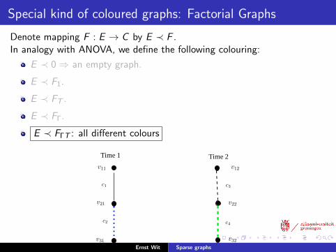
Special kind of coloured graphs: Factorial Graphs

Denote mapping F : E → C by E ≺ F .In analogy with ANOVA, we define the following colouring:

E ≺ 0⇒ an empty graph.

E ≺ F1.

E ≺ FT .

E ≺ FΓ.

E ≺ FΓT .

v12

v22

v32

Time 1 Time 2

v11

v21

v31





E ≺ F1: same colour for all links

E ≺ FT .

E ≺ FΓ.

E ≺ FΓT .

v12

v22

v32

Time 1 Time 2

v11

v21

v31

c1





E ≺ F1.

E ≺ FT : same colour across all genes

E ≺ FΓ.

E ≺ FΓT .

v12

v22

v32

Time 1 Time 2

v11

v21

v31

c1 c2





E ≺ F1.

E ≺ FT .

E ≺ FΓ: same colour across all times

E ≺ FΓT .

v12

v22

v32

Time 1 Time 2

v11

v21

v31

c1

c2





E ≺ F1.

E ≺ FT .

E ≺ FΓ.

E ≺ FΓT : all different colours

v12

v22

v32

Time 1 Time 2

v11

v21

v31

c3c1

c2 c4


Natural Partitions

Definition (Natural partition)

Let E = {Si ,Ni}nT−1i=0 be subsets of links where Si ,Ni are defined as follows:

Si = {{(vjt , vj,t+i ), (vj,t+i , vjt)}|j ∈ Γ, t = 1, . . . , nT − i},

andNi = {{(vjt , vk,t+i ), (vk,t+i , vjt)}|∀j 6= k ∈ Γ, t = 1, . . . , nT − i}.

The natural partitions imply subgraphs of G and imply partions of Θ for GGMs:

Θ =

S0 N0 S1 N1 S2 N2 . . . . . .

S0 N1 S1 N2 S2 . . . . . .S0 N0 S1 N1 S2 N2

S0 N1 S1 N2 S2

S0 N0 S1 N1

S0 N1 S1


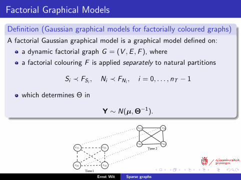
Factorial Graphical Models

Definition (Gaussian graphical models for factorially coloured graphs)

A factorial Gaussian graphical model is a graphical model defined on:

a dynamic factorial graph G = (V ,E ,F ), where

a factorial colouring F is applied separately to natural partitions

Si ≺ FSi , Ni ≺ FNi, i = 0, . . . , nT − 1

which determines Θ in

Y ∼ N(µ,Θ−1).

Time1

Time 2v11 v21

v31 v41

v12 v22

v32 v42


Example: Factorial Gaussian Graphical Model

Model:

(S0 ≺ 1), N0 ≺ FT , S1 ≺ 1, N1 ≺ 0.

Factorial coloured graph:

Time1

Time 2v11 v21

v31 v41

v12 v22

v32 v42

Precision Matrix:

Θ =

θ1 θ2 θ2 θ2 θ4 0 0 0θ1 θ2 θ2 0 θ4 0 0

θ1 θ2 0 0 θ4 0θ1 0 0 0 θ4

θ1 θ3 θ3 θ3

θ1 θ3 θ3

θ1 θ3

θ1


Penalized likelihood for GGMs

Consider an experiment: |Γ| genes measured across |T | time points.

Assume n iid samples y(1), . . . , y(n), where y(i) = (y(i)1 , . . . , y

(i)ΓT ).

Assume Y(i) ∼ N(0,Θ−1), then

Likelihood:l(Θ|y) ∝ log(Θ)− tr(SΘ).

AIM: Optimization of penalized likelihood:

Θ̂ := argmaxΘ{l(Θ|y)}

subject to

Θ � 0;

||Θ||1 ≤ 1/λ;

some factorial colouring F .


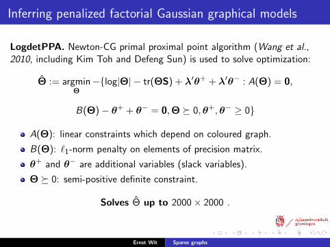
Inferring penalized factorial Gaussian graphical models

LogdetPPA. Newton-CG primal proximal point algorithm (Wang et al.,2010, including Kim Toh and Defeng Sun) is used to solve optimization:

Θ̂ := argminΘ−{log|Θ| − tr(ΘS) + λ′θ+ + λ′θ− : A(Θ) = 0,

B(Θ)− θ+ + θ− = 0,Θ � 0,θ+,θ− ≥ 0}

A(Θ): linear constraints which depend on coloured graph.

B(Θ): `1-norm penalty on elements of precision matrix.

θ+ and θ− are additional variables (slack variables).

Θ � 0: semi-positive definite constraint.

Solves Θ̂ up to 2000× 2000 .


T-cell data

Aim. Use large time-course experiment to characterize response of humanT-cell line (Jurkat) to PMA and ionomycin treatment.

T-cell time-series dataset

Temporal expression of 58 genes for 10 unequally spaced time points.

At each time point there are 44 separate measurements.

See Rangel et al. (2004) for more details.


Application to T-cell data

S0 ≺ F1,N0 ≺ FΓ,S1 ≺ FT ,N1 ≺ FΓ

Θ =

S1

0 N10 S1

1 N11 0 0 . . . . . .

S10 N1

1 S11 0 0 . . . . . .

S20 N2

0 S21 N2

1 0 0S2

0 N21 S2

1 0 0S3

0 N30 S3

1 N31

S30 N3

1 S31

N1

0 = N20 = . . . = N10

0 N11 = N2

1 = . . . = N101

RB1

SIVA

LCK

ITGAM

SMN1

CASP8

PCNA

CCNC

PDE4B

APC

ID3

CDK4

TCF12

CDC2

CCNA2

PIG3

CASP4

TCF8

GATA3

CSF2RA

MPO

CYP19

CASP7

JUNB

NFKBIA

RB1

SIVA

ITGAM

SMN1

PCNA

CCNC

ID3

SLA

CDK4

TCF12

MCL1

CDC2

CCNA2

MYD88

TCF8

GATA3

IL2RG

CSF2RA

MPO

CYP19

CASP7

JUNBNFKBIA


What have we achieved so far? And problems!

Summary:

Penalized Gaussian graphical models

Coloured graphs

Natural partitions

Factorially coloured Gaussian graphical models

Problems:

1 Factorial colouring not particularly flexible in modeling time dynamics.

2 Gaussian assumption may be too restrictive for realistic genomic data.

3 How to choose the appropriate level of penalization?


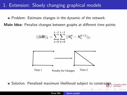
1. Extension: Slowly changing graphical models

Problem: Estimate changes in the dynamic of the network.

Main Idea: Penalize changes between graphs at different time points

||∆Θ||1 =t−1∑s=0

t−1∑k=0

||Nks − Nk+1

s ||1.

b b

bb

b b

bb

Penalty for ChangesTime 1 Time 2

Solution: Penalized maximum likelihood subject to constraints.


Implement Slowly Changing via logdetPPA

Θ̂ := argminΘ{− log |Θ|+ tr(SΘ) + λ1x+ + λ1x− + λ2y+ + λ2y−}

subject to A(Θ)− y+ + y− = 0

B(Θ)− x+ + x− = 0

C(Θ) = 0

Θ � 0, x+, x−, y+, y− ≥ 0.

A(Θ): set of linear constraints which depends on the ||∆Θ||1.

B(Θ) `1-norm penalty on element of precision matrix.

C (Θ) zero elements a priori.

x+, x−, y− and y+ are slack variables.


Application to a time-course dataset

S0 ≺ FΓT ,N0 ≺ 1,N1 ≺ 1,N2 ≺ 0

Θ =

S1

0 N10 S1

1 N11 0 0 . . . . . .

S10 N1

1 S11 0 0 . . . . . .

S20 N2

0 S21 N2

1 0 0S2

0 N21 S2

1 0 0S3

0 N30 S3

1 N31

S30 N3

1 S31

N1

0 |N10 | − |N2

0 | |N20 | − |N3

0 |N0 at time 1

NMB0886

NMB1980

NMB1378NMB1401

NMB0102

NMB1321

NMB0046

NMB0438

NMB0125

NMB0888

NMB1322

NMB1811

NMB2141

NMB1312

NMB0211

NMB0889

NMB1437

NMB0206

NMB1580

NMB1808

NMB1857

NMB1728

NMB0467

NMB1377

NMB0035

NMB1394

NMB0568

NMB2037

NMB0720

NMB0559

NMB1342

NMB1058

NMB1809

NMB0700

NMB1973

NMB0944

NMB1812

NMB2038

NMB0926

NMB1053 NMB0721

NMB0791

NMB1458

NMB1541

NMB1810

NMB1636

NMB1972

NMB0744

1

NMB0886NMB0125

NMB0888NMB1580

NMB0926

NMB1053

NMB0721

NMB1810

NMB1636

NMB0744

7

NMB1321

NMB1857

NMB0926

NMB1053


2. Extension: Non-Normality

Problem: Non-Normality of the data (e.g. T-cell).

19.5 20.0 20.5

0.00.5

1.01.5

2.0

FYB

Densi

ty

18.2 18.6 19.0

0.00.5

1.01.5

2.02.5

MPO

Densi

ty

15.5 16.5 17.5

0.00.5

1.01.5

2.02.5

3.03.5

MCL1

Densi

tySolution: Copula Gaussian graphical models


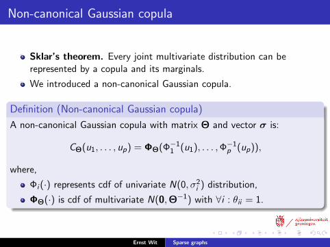
Non-canonical Gaussian copula

Sklar’s theorem. Every joint multivariate distribution can berepresented by a copula and its marginals.

We introduced a non-canonical Gaussian copula.

Definition (Non-canonical Gaussian copula)

A non-canonical Gaussian copula with matrix Θ and vector σ is:

CΘ(u1, . . . , up) = ΦΘ(Φ−11 (u1), . . . ,Φ−1

p (up)),

where,

Φi (·) represents cdf of univariate N(0, σ2i ) distribution,

ΦΘ(·) is cdf of multivariate N(0,Θ−1) with ∀i : θii = 1.


Copula Gaussian graphical models

IDEA:

Graph exists on a hidden Gaussian variable Z ∼ N(0,Θ),

Z gives rise to observed non-Gaussian data Y.

b

b

b

b

b

b

b

v1v2

v3

v4v5

v6v7

F1

F2

F7

Marginal Distribution: F

...

Y1 = F−11 (φ(Z1))

Y2 = F−12 (φ(Z2))

Y7 = F−1p (φ(Z7))

...

Observed: YLatent Variable: Z ∼ N(µ,Θ−1)

We consider the Fi as nuisance parameters.

For continuous variables: 1-to-1 relationship between Z and Y .For discrete variables, relationship is more complicated!


Gaussian Copula for Ordinal Variables

If Y = (Y1, . . . ,Yp) consist of ordinal variables, e.g.,

Yi ∈ {1, 2, 3, 4}, severity score for item i

Assume existence latent variable Z = (Z1, . . . ,Zp) ∼ N(0,Θ−1), such that

Y(k)i < Y

(l)i ⇐⇒ Z

(k)i < Z

(l)i .

−3 −2 −1 0 1 2 3

0.0

0.1

0.2

0.3

0.4

P Y 1=0

P Y 1=1

P Y 1=2

P Y 1=3

P Y 1=4

−1 0 1 2 3 4 5

0.0

0.2

0.4

0.6

0.8

1.0

y

F̂(y

)●

●

●

●

●

Values of zi that correspond to yi ,

D(yi ) = {z ∈ R | F−1i (Φi (z)) = yi}


Maximum Likelihood Estimation

Gaussian copula density function is:

φΘ(u) = |Θ|1/2exp(−1

2Φ−1(u)′(Θ− I)Φ−1(u)),

u = F(z) = (F1(z1), . . . ,Fp(zp))

The profile marginal likelihood is:

L(Θ|D, F̂1, . . . , F̂p) =

∫z∈D

φΘ(z)dz

Problem: Marginal likelihood is hard.


Solution: The iterative EM Algorithm

E-Step: Compute the quantity Q(Θ|Θ(m)) = EZ[l(Θ)|Y,Θ(m)]

Q(Θ | Θ(m)) = E

[n∑

i=1

(1

2log |Θ| − 1

2Z′iΘZi +

1

2Z′iZi

)| yi ,Θ(m)

]

=n

2

{log |Θ| − 1

n

n∑i=1

tr(

ΘE[ZiZ

′i | Zi ∈ D(Yi ),Θ

(m)])

+1

n

n∑i=1

tr(E[ZiZ

′i | Zi ∈ D(Yi ),Θ

(m)])}

=n

2

{log |Θ| − tr

(ΘR̄)

+ tr(R̄)},

R̄ = E[ZiZ

′i | Zi ∈ D(Yi ),Θ

(m)].

M-Step: Maximize the quantity Q(Θ|Θ(m)) subject to ||Θ||1 ≤ 1/λ andcolouring F .

Problem: Obtaining the quantity E[ZiZ

′i | Zi ∈ D(Yi ),Θ

(m)].


Wilhem, S. and Manjunath, B. (2010)

The second moment is:

R̄ = E[ZsZt | (L,U) ∈ D,Θ(m)

]=

p∑k=1

ρ(m)sk ρ

(m)tk [LkGk(Lk)− UkGk(Uk)]

+

p∑k=1

ρ(m)tk

∑l 6=k

(ρ

(m)tl − ρ

(m)kl ρ

(m)tk

)× {[Gkl(Lk , Ll)− Gkl(Lk ,Ul)]

− [Gkl(Uk , Ll)− Gkl(Uk , Ll)]}Compute

Gk(zk) =

∫ U1

L1

· · ·∫ Uk−1

Lk−1

∫ Uk+1

Lk+1

· · ·∫ Up

Lp

φp(zk , z−k | Θ(m))dz−k

Gkl(zk , zl) =

∫ U1

L1

· · ·∫ Uk−1

Lk−1

∫ Uk+1

Lk+1

· · ·∫ Ul−1

Ll−1

∫ Ul+1

Ll+1

· · ·∫ Up

Lp

φp(zk , zl , z−k,−l | Θ(m))dz−k,−l ,


Application of Gaussian copula graphical models to T-cell

S0 ≺ F1,N0 ≺ FΓ,S1 ≺ FT ,N1 ≺ FΓ

RB1

MAPK9

SMN1

E2F4

CCNC

APC

TCF12

CCNA2

CASP4

TCF8

GATA3

CSF2RA

CYP19

JUNB

RB1

MAPK9

JUND

ITGAM

SMN1CCNC

APC

TCF12 CCNA2

PIG3

CASP4TCF8

GATA3

CSF2RA

MPO

CYP19

JUNB

N10 = N2

0 = . . . = N100 N1

1 = N21 = . . . = N10

1


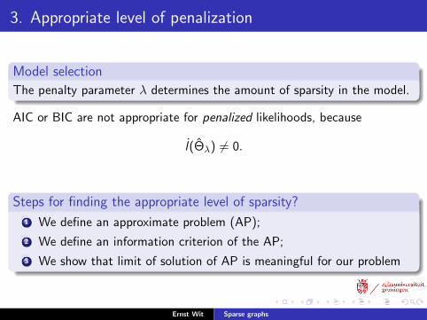
3. Appropriate level of penalization

Model selection

The penalty parameter λ determines the amount of sparsity in the model.

AIC or BIC are not appropriate for penalized likelihoods, because

l̇(Θ̂λ) 6= 0.

Steps for finding the appropriate level of sparsity?

1 We define an approximate problem (AP);

2 We define an information criterion of the AP;

3 We show that limit of solution of AP is meaningful for our problem


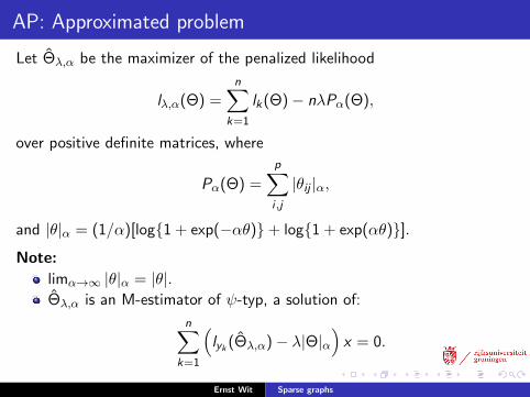
AP: Approximated problem

Let Θ̂λ,α be the maximizer of the penalized likelihood

lλ,α(Θ) =n∑

k=1

lk(Θ)− nλPα(Θ),

over positive definite matrices, where

Pα(Θ) =

p∑i ,j

|θij |α,

and |θ|α = (1/α)[log{1 + exp(−αθ)}+ log{1 + exp(αθ)}].Note:

limα→∞ |θ|α = |θ|.Θ̂λ,α is an M-estimator of ψ-typ, a solution of:

n∑k=1

(lyk (Θ̂λ,α)− λ|Θ|α

)x = 0.


GIC for Approximated Problem

Konishi and Kitagawa (2008) defined the GIC for M-estimators:

GIC (Θ̂λ,α) = −n{log |Θ̂λ,α| − Tr(Θ̂λ,αS)}+ 2Tr{R−1(α)Q},

where R(α) is square matrix of order p2

R(α) =1

2Θ̂−1λ,α ⊗ Θ̂−1

λ,α + λP ′′α(Θ̂λ,α), (1)

and P ′′α(q̂λ,α) diagonal matrix with p2 elements (|θ̂11|′′α, θ̂12|′′α, . . . , |θ̂pp|′′α)and

Q(α) =1

4vectSvectST − 1

4n

n∑k=1

vectkvectTk

= Q


Limit of AP approximation GIC

The L1 penalized estmimators are no M-estimators, so K&K GIC is notdefined. We define the GIC as the limit of the approximated one.

Definition (“GIC” for L1 penalized graphical models.)

GIC(λ) = −n{log |Θ̂λ| − Tr(Θ̂λS)}+ 2Tr(R−1Q),

Matrix Q is square matrix of order p2 (as above) and

R[I , I ] = Θ̂λ ⊗ Θ̂λ[I , I ]−1,

where I are the non-zero elements in vectΘ̂λ.


Performance of the GIC: simulation study

N = 8

TP Sens. TN Spec. MCC Accuracy

GIC 13.0 0.531 51.0 0.543 0.044 0.545(4.9) (0.203) (16.3) (0.173) (0.088) (0.102)

AIC 0.0 0.000 94.0 1.000 0.000 0.783(2.1) (0.090) (7.6) (0.081) (0.057) (0.045)

BIC 0.0 0.000 94.0 1.000 0.000 0.783(1.6) (0.076) (6.1) (0.065) (0.057) (0.035)

N = 12

GIC 16.0 0.667 45.0 0.479 0.120 0.517(4.3) (0.176) (13.8) (0.147) (0.092) (0.090)

AIC 2.0 0.077 93.0 0.989 0.093 0.783(6.5) (0.264) (19.8) (0.211) (0.099) (0.112)

BIC 0.5 0.019 94.0 1.000 0.008 0.783(0.9) (0.038) (1.1) (0.011) (0.095) (0.008)

Results p = 16; Present Links = 26; Absent Links=102


Conclusion and Discussion

Summary:

Factorial graphical models based on coloured graphs.

Slowly changing graphical models.

Extension: Copula Gaussian graphical models.

How do we evaluate model complexity?

Questions:

How would we adapt model with other factors?

Could we combine Copulas with slowly changing networks?

How to introduce latent structures?


Documents

Sparse Graphs (from noisy data, obviously)Sparse Graphs (from noisy data, obviously) Ernst Wit Johann Bernoulli Institute University of Groningen October 4, 2012 Ernst Wit Sparse graphs