Sparse Gaussian Elimination modulo p:an Update

Charles Bouillaguet1 and Claire Delaplace1,2

1 Univ. Lille, CNRS, Centrale Lille, UMR 9189 - CRIStAL - Centre de Recherche enInformatique Signal et Automatique de Lille, F-59000 Lille, France

charles.bouillaguet@univ-lille1.fr2 Université de Rennes-1 / IRISA

claire.delaplace@irisa.fr

Abstract. This paper considers elimination algorithms for sparse matri-ces over finite fields. We mostly focus on computing the rank, because itraises the same challenges as solving linear systems, while being slightlysimpler.We developed a new sparse elimination algorithm inspired by the Gilbert-Peierls sparse LU factorization, which is well-known in the numericalcomputation community. We benchmarked it against the usual right-looking sparse gaussian elimination and the Wiedemann algorithm usingthe Sparse Integer Matrix Collection of Jean-Guillaume Dumas.We obtain large speedups (1000× and more) on many cases. In particu-lar, we are able to compute the rank of several large sparse matrices inseconds or minutes, compared to days with previous methods.

1 Introduction

There are essentially two families of algorithms to perform the usual operationson sparse matrices (rank, determinant, solution of linear equations, etc.): directand iterative methods.

Direct methods (such as gaussian elimination, LU factorization, etc.) gener-ally produce an echelonized version of the original matrix. This process oftenincurs fill-in: the echelonized version has more non-zero entries than the origi-nal. Fill-in increases the time and space needed to complete the echelonization.As such, the time and space requirements of direct methods are usually unpre-dictable; they may fail if not enough storage is available, or become excruciat-ingly slow.

Iterative methods such as theWiedemann algorithm [29] only perform matrix-vector products and only need to store one or two vectors in addition to thematrix. They do not incur any fill-in. On rank-r matrices, the number of matrix-vector products that must be performed is 2r. Also, when a matrix M has |M |non-zero entries, computing the matrix-vector product x ·M requires O (|M |)operations. The time complexity of iterative methods is thus O (r|M |), whichis fairly easy to predict, and the space complexity is essentially that of keeping

2 Charles Bouillaguet and Claire Delaplace

the matrix in memory. These methods are often the only option for very largematrices, or for matrices where fill-in makes direct methods impractical.

In a paper from 2002, Dumas and Villard [15] surveyed and benchmarkedalgorithms dedicated to rank computations for sparse matrices modulo a smallprime number p. In particular, they compared the efficiency of sparse gaussianelimination and the Wiedemann algorithm on a collection of benchmark matricesthat they collected from other researchers and made available on the web [16].They observed that while iterative methods are fail-safe and can be practical,direct methods can sometimes be much faster. This is in particular the case whenmatrices are almost triangular, so that gaussian elimination barely has anythingto do.

It follows that both methods are worth trying. In practical situations, apossible workflow could be : “try a direct method ; if there is too much fill-in,abort and restart with an iterative method ”.

We concur with the authors of [15], and strengthen their conclusion by devel-oping a new sparse elimination algorithm which outperforms all other techniquesin some cases, including several large matrices which could only be processed byan iterative algorithm.

Lastly, it is well-known that both methods can be combined: performing onestep of elimination reduces the size of the “remaining” matrix (the Schur comple-ment) by one, while increasing the number of non-zeros. This may decrease thetime complexity of running an iterative method on the Schur complement. Thisstrategy can be implemented as follows: “While the product of the number of re-maining rows and remaining non-zeros decreases, perform an elimination step ;then switch to an iterative method ”. For instance, one phase of the record-settingfactorization of a 768-bit number [20] was to find a few vectors on the kernelof a 2 458 248 361 × 1 697 618 199 very sparse matrix over F2 (with about 30non-zero per row). A first pass of elimination steps (and discarding “bad” rows)reduced this to a roughly square matrix of size 192 796 550 with about 144 non-zero per row. A parallel implementation of the block-Wiedemann [7] algorithmthen finished the job. The algorithm presented in this paper lends itself well tothis hybridization.

1.1 Our contribution

Our original intention was to check whether the conclusions of [15] could berefined by using more sophisticated sparse elimination techniques used in thenumerical world. To do so, we developed the SpaSM software library (SPArseSolver Modulo p). Its code is publicly available in a repository hosted at:

https://github.com/cbouilla/spasm

Our code is heavily inspired by CSPARSE (“A Concise Sparse Matrix Packagein C ”), written by Davis and abundantly described in his book [9]. We modifiedit to work row-wise (as opposed to column-wise), and more importantly to dealwith non-square or singular matrices. At its heart lies a sparse LU factorization

Sparse Gaussian Elimination modulo p: an Update 3

algorithm. It is capable of computing the rank of a matrix, but also of solvinglinear systems (and, with minor adaptations, of computing the determinant,finding a basis of the kernel, etc.).

We used this as a playground to implement the algorithms described in thispaper —as well as some other, less successful ones. This was necessary to testtheir efficiency in practice. We benchmarked them using matrices from Dumas’scollection [16], and compared them with the algorithms used in [15], which arepublicly available inside the LinBox library. This includes a right-looking sparsegaussian elimination, and the Wiedemann algorithm.

There are several cases where the algorithm described in section 3 achievea 1000× speedup compared to previous algorithms. In particular, it systemati-cally outperforms the right-looking sparse gaussian elimination implemented inLinBox.

It is capable of computing the rank of several of the largest matrices from [16],where previous elimination algorithms failed. In these cases, it vastly outperformsthe Wiedmann algorithm. In a striking example, two computations that requiredtwo days with the Wiedemann algorithm could be performed in 30 minutes and30 seconds respectively using the new algorithm. More complete benchmarkresults are given in section 4.

We relied on three main ideas to obtain these results. First, we built uponGPLU [19], a left-looking sparse LU factorization algorithm. We then used asimple pivot-selection heuristic designed in the context of Gröbner basis compu-tation [18], which works well with left-looking algorithms. On top of these twoideas, we designed a new, hybrid, left-and-right looking algorithm.

Our intention is not to develop a competitor sparse linear algebra library; weplan to contribute to LinBox, but we wanted to check the viability of our ideasfirst.

1.2 Related Work

Sparse Rank Computation mod p. Our starting point was [15], where aright-looking sparse gaussian elimination and theWiedemann algorithm are com-pared on many benchmark matrices. [23,24] consider the problem of large densematrices of small rank modulo a very small prime, while [25] shows that mostoperations on extremely sparse matrices with only two non-zero entries per rowcan be performed in time O (n). [17] discusses sparse rank computation of thelargest matrices of our benchmark collection by various methods. The largestcomputation were performed with a parallel block-variant of the Wiedemannalgorithm.

Direct Methods in the Numerical World. A large body of work hasbeen dedicated to sparse direct methods by the numerical computation com-munity. Direct sparse numerical solvers have been developped during the 1970’s,so that several software packages were ready-to-use in the early 1980’s (MA28,

4 Charles Bouillaguet and Claire Delaplace

SPARSPAK, YSMP, ...). For instance, MA28 is an early “right-looking” (cf. sec-tion 2) sparse LU factorization code described in [12,13]. It uses Markowitzpivoting [22] to choose pivots in a way that maintains sparsity.

Most of these direct solvers start with a symbolic analysis phase that ignoresthe numerical values and just examines the pattern of the matrix. Its purpose isto predict the amount of fill-in that is likely to occur, and to pre-allocate datastructures to hold the result of the numerical computation. The complexity ofthis step often dominated the running time of early sparse codes. In addition, animportant step was to choose a priori an order in which the rows (or columns)were to be processed in order to maintain sparsity.

Sparse linear algebra often suffers from poor computational efficiency, be-cause of irregular memory accesses and cache misses. More sophisticated directsolvers try to counter this by using dense linear algebra kernels (the BLAS andLAPACK) which have a much higher FLOP per second rate.

The supernodal method [6] does this by clustering together rows (or columns)with similar sparsity pattern, yielding the so-called supernodes, and process-ing them all at once using dense techniques. Modern supernodal codes includeCHOLDMOD [5] (for Cholesky factorization) and SuperLU [11]. The former isused in Matlab on symmetric positive definite matrices.

In the same vein, the multifrontal method [14] turns the computation of asparse LU factorization into several, hopefully small, dense LU factorizations.The starting point of this method is the observation that the elimination of apivot creates a completely dense submatrix in the Schur complement. Contem-porary implementations of this method are UMFPACK [8] and MUMPS [1]. Theformer is also used in Matlab in non-symmetric matrices.

Finally, “left-looking” algorithms are those that do not explicitly computethe Schur complement during the sparse factorization. This is for instance thecase of SPARSPAK cited earlier. A very interesting algorithm, referred to asGPLU [19], computes an LU factorization in time proportionnal to the numberof arithmetic operations needed to compute the product L × U (assuming thezeros are not stored). In particular, the symbolic part of the factorization doesnot dominate the numerical part asymptotically. This algorithm is implementedin Matlab, and is used for very sparse unsymmetric matrices. It is also the heartof the specialized library called KLU [10], dedicated to circuit simulation.

Direct Methods Modulo p. The world of exact sparse direct methods is muchless populated. Besides LinBox, we are not aware of many implementations ofsparse gaussian elimination capable of computing the rank of a matrix modulo p.According to its handbook, the MAGMA [2] computer algebra system computesthe rank of a sparse matrix by first performing sparse gaussian elimination withMarkowitz pivoting, then switching to a dense factorization when the matrixbecomes dense enough. The Sage [28] system uses LinBox.

Some specific applications rely on exact sparse linear algebra. All competitivefactoring and discrete logarithms algorithms work by finding a few vectors in thekernel of a large sparse matrix. Some controlled elimination steps are usually

Sparse Gaussian Elimination modulo p: an Update 5

performed, which makes the matrix smaller and denser. This has been called“structured gaussian elimination” [21]. The process can be continued until thematrix is fully dense (after which it is handled by a dense solver), or stoppedearlier, when the resulting matrix is handled by an iterative algorithm. Thecurrent state-of-the-art factoring codes, such as CADO-NFS [26], seem to use thesparse elimination techniques described in [4].

Modern Gröbner basis algorithms work by computing the reduced row-echelonform of particular sparse matrices. An ad hoc algorithm has been designed, ex-ploiting the mostly triangular structure of these matrices to find pivots withoutperforming any computation [18]. An open-source implementation, GBLA [3], isavailable.

2 Sparse LU Factorization

In this section we discuss algorithms to compute a sparse LU factorization of amatrix A of size n×m over a finite field. The techniques described in this papercould in principle work over any field; for the sake of simplicity we focus on thecase of integers modulo a prime p that fits into a machine integer.

2.1 Definitions and Notations

We recall here some usefull definitions. A is an n-by-m matrix and its (unknown)rank is denoted by r.

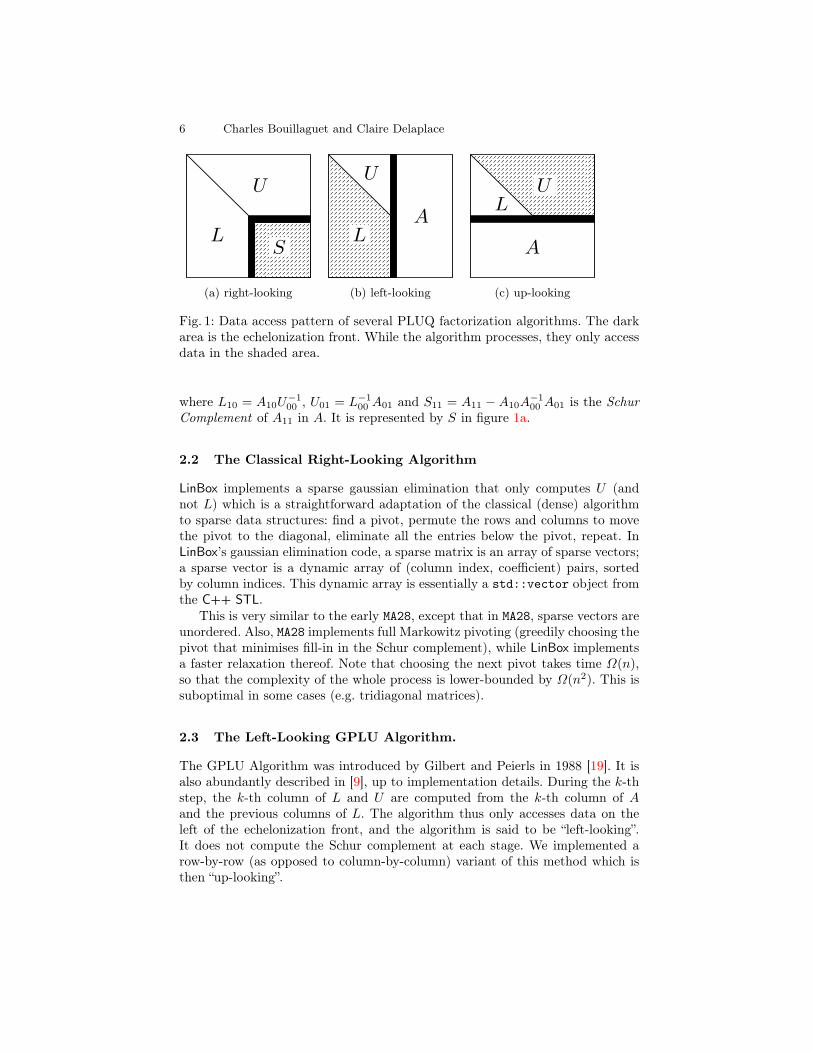
Because A is rectangular, we consider the PLUQ factorization of A whereL is n-by-r and lower-trapezoidal with a unit diagonal, U is r-by-m and upper-trapezoidal with a non-zero diagonal and P (resp. Q) is a permutation over therows (resp. columns) of A. Computing a PLUQ factorization essentially amountsto performing gaussian elimination. We recall the usual (dense) algorithm: ateach step i, choose a coefficient aik 6= 0 called the pivot and “eliminate” everycoefficients under it by adding suitable multiples of row i to the rows below.This method is said to be right-looking, because at each step it accesses thedata stored in the bottom-right of A (shaded aera in figure 1a). This contrastswith left-looking algorithms (or the up-looking row-by-row equivalent describedin section 2.3), that accesses the data stored in the left of L (respectively in thetop of U) represented by the shaded aera in figure 1b (1c).

If we assume that we have performed some steps of the PLUQ decomposition,then we have

PAQ =

(A00 A01

A10 A11

),

such that A00 is square, nonsingular and can be factored as A00 = L00 · U00. Itleads to the following factorization of A :

PAQ =

(L00

L10 I

)·(U00 U10

S11

),

6 Charles Bouillaguet and Claire Delaplace

L

U

S

(a) right-looking

L

U

A

(b) left-looking

LU

A

(c) up-looking

Fig. 1: Data access pattern of several PLUQ factorization algorithms. The darkarea is the echelonization front. While the algorithm processes, they only accessdata in the shaded area.

where L10 = A10U−100 , U01 = L−1

00 A01 and S11 = A11 − A10A−100 A01 is the Schur

Complement of A11 in A. It is represented by S in figure 1a.

2.2 The Classical Right-Looking Algorithm

LinBox implements a sparse gaussian elimination that only computes U (andnot L) which is a straightforward adaptation of the classical (dense) algorithmto sparse data structures: find a pivot, permute the rows and columns to movethe pivot to the diagonal, eliminate all the entries below the pivot, repeat. InLinBox’s gaussian elimination code, a sparse matrix is an array of sparse vectors;a sparse vector is a dynamic array of (column index, coefficient) pairs, sortedby column indices. This dynamic array is essentially a std::vector object fromthe C++ STL.

This is very similar to the early MA28, except that in MA28, sparse vectors areunordered. Also, MA28 implements full Markowitz pivoting (greedily choosing thepivot that minimises fill-in in the Schur complement), while LinBox implementsa faster relaxation thereof. Note that choosing the next pivot takes time Ω(n),so that the complexity of the whole process is lower-bounded by Ω(n2). This issuboptimal in some cases (e.g. tridiagonal matrices).

2.3 The Left-Looking GPLU Algorithm.

The GPLU Algorithm was introduced by Gilbert and Peierls in 1988 [19]. It isalso abundantly described in [9], up to implementation details. During the k-thstep, the k-th column of L and U are computed from the k-th column of Aand the previous columns of L. The algorithm thus only accesses data on theleft of the echelonization front, and the algorithm is said to be “left-looking”.It does not compute the Schur complement at each stage. We implemented arow-by-row (as opposed to column-by-column) variant of this method which isthen “up-looking”.

Sparse Gaussian Elimination modulo p: an Update 7

The main idea behind the algorithm is that the next row of L and U canboth be computed by solving a triangular system. If we ignore row and col-umn permutations, this can be derived from the following 3-by-3 block matrixexpression : L00

l10 1L20 l21 L22

U00 u01 U02

u11 u12

U22

=

A00 a01 A02

a10 a11 a12A20 a21 A22

.

Here (a10 a11 a12) is the k-th row of A. L is assumed to have unit diagonal.Assume we have already computed (U00 u01 U02), the first k rows of U . Thenwe have: (

l10 u11 u12

)·

U00 u01 U02

1Id

=(a01 a11 a21

). (1)

Thus, the whole PLUQ factorization can be performed by solving a sequence ofn sparse triangular systems.

Sparse Triangular Solving. To make the above idea work, we need to solveefficiently x ·U = b, where U is a sparse matrix stored by rows, and b is a sparsevector (a row of A). The main trick of the GPLU algorithm is that it is possibleto determine the sparsity pattern of x without performing any kind of numericalcomputation.

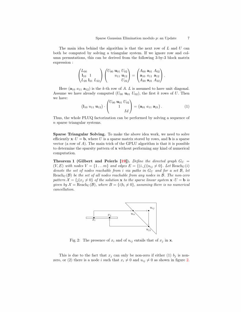
Theorem 1 (Gilbert and Peierls [19]). Define the directed graph GU =(V,E) with nodes V = 1 . . .m and edges E = (i, j)|uij 6= 0. Let ReachU (i)denote the set of nodes reachable from i via paths in GU and for a set B, letReachU (B) be the set of all nodes reachable from any nodes in B. The non-zeropattern X = j|xj 6= 0 of the solution x to the sparse linear system x ·U = b isgiven by X = ReachU (B), where B = i|bi 6= 0, assuming there is no numericalcancellation.

xi

xjuii

uij

ujj

Fig. 2: The presence of xi and of uij entails that of xj in x.

This is due to the fact that xj can only be non-zero if either (1) bj is non-zero, or (2) there is a node i such that xi 6= 0 and uij 6= 0 as shown in figure 2.

8 Charles Bouillaguet and Claire Delaplace

Thus, X can be determined by performing a graph traversal in GU starting fromeach node of B. If we perform a depth-first search, then we will naturally obtainX sorted in topological order : if uij 6= 0, then i comes up before j in X . Thisenables the following efficient procedure to compute x:1: Scatter b into a (dense) working array w, initially filled with 0.2: for all i ∈ X in topological order do3: wi ← wi/uii4: for all j > i such that uij 6= 0 do5: wj ← wj − wiuij

6: Gather x (get wi for i ∈ X ), and reset w.

A striking feature of this triangular solver is that it may terminate in constanttime in some cases (for instance if U is bidiagonal, and b has only a constantnumber of entries). In addition, the complexity of finding X is of the same orderas that of the numerical computation of x once X is known: each iteration ofline 5 in the above pseudo-code corresponds to the crossing of an edge in GU

during the construction of X . This holds well in our implementation: computingX consistenty requires 25% of the time needed to compute x.

Selecting the Pivots. For the triangular systems to have a solution, we need tomake sure that the diagonal coefficient of U (the pivots) are non-zero. However,while solving the system (1), we may find u11 = 0. There are two possible cases:(1) If u11 = 0 and u12 6= 0, then we can permute the column j0 where u11 iswith another one j1, such that j0 < j1. (2) If u11 = 0 and u12 = 0, then there isno way we can permute the columns of U to bring a non-zero coefficent on thediagonal. This means that the current row of A is a linear combinations of theprevious rows. When the factorization is done, the number of non-empty rowsof U is the rank r of the matrix A.

Useful Heuristics. Right-looking algorithms have the possibility to choose thenext pivot by exploiting knowledge of the Schur complement (this is typicallywhat Markowitz pivoting is about). On the other hand, the only informationavailable to left-looking algorithms such as GPLU to choose pivots is the origi-nal matrix, and the part of U that has already been computed. It is possible tochoose an a priori order in which to process the rows of the matrix in order tokeep U as sparse as possible. Many different strategies have been designed to doso in the numerical world: the (approximate) minimum degree algorithm, nesteddissection, etc. The problem is that these algorithms are mostly adapted to sym-metric matrices, and a fortiori to square matrices. They are usually retrofittedto the unsymmetric case by applying them to ATA, which is square and sym-metric. However, when A is very rectangular, this becomes completely dense andprovide little useful information.

We instead implemented a much simpler heuristic inspired from an echel-onization procedure dedicated to Gröbner basis computation by Faugère andLachartre [18]. We map each row to the column of its leftmost coefficient. When

Sparse Gaussian Elimination modulo p: an Update 9

several rows have the same leftmost coefficient, we select the sparsest row. Wethen move the selected rows before the others and sort them by increasing po-sition of the left-most coefficient. As a result, the leftmost coefficient of eachrow cannot occur in any selected row below it. It follows that the selected rowsare copied as-is into U , with zero fill-in. This is particularly well-suited to theGPLU algorithm, because this keeps U as sparse as possible; this in turn makesthe triangular solver fast.

Also, we observed that it can be beneficial to compute the rank of the trans-pose of the matrix. Indeed, U has size r ×m, so when m is much larger thann, transposing the matrix before starting the computation ensures than U issmaller. More often than not this decreases the running time of the factoriza-tion (on the matrices from [16]). Lastly, we note that the running time of theright-looking algorithm implemented in LinBox is usually not the same on A andAT .

We also implemented a simple early abort test which is performed whensufficiently many rows have been processed without finding any new pivot. Arandom linear combination of the remaining rows is computed; if it belongs tothe row-space of U , then no new pivot will be found in the remaining rows withprobability greater than 1−1/p. This test can be repeated to increase its successprobability exponentially.

2.4 Left or Right?

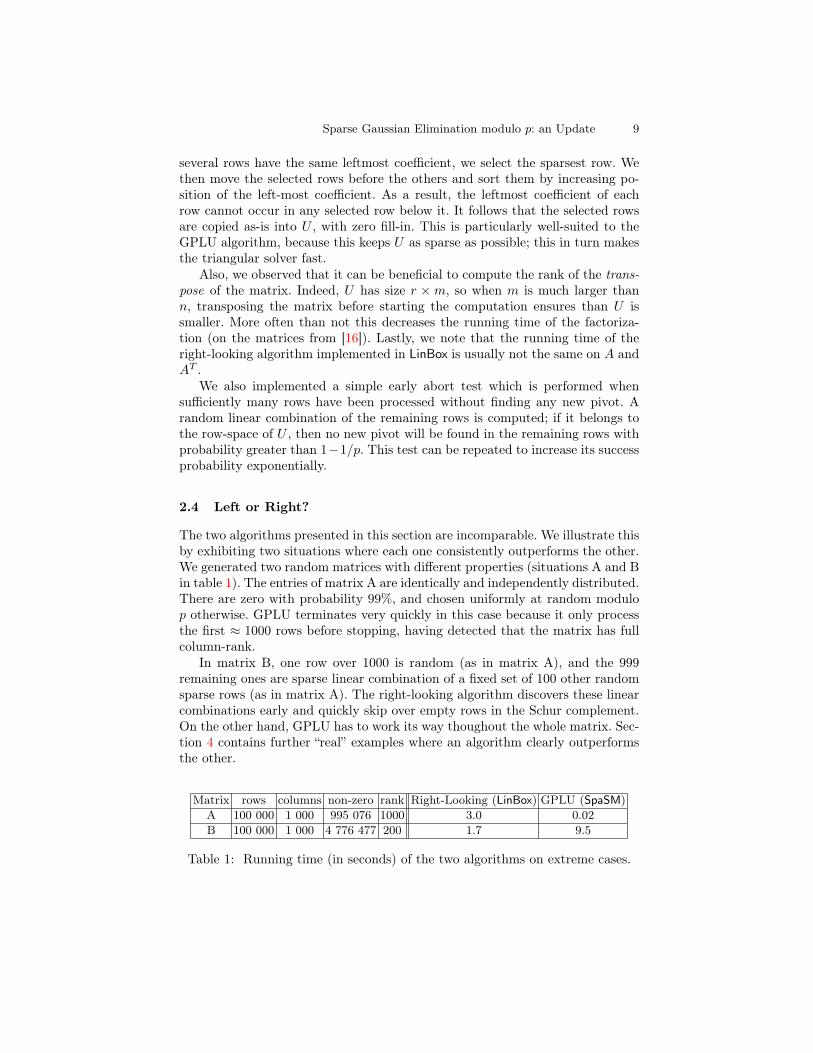
The two algorithms presented in this section are incomparable. We illustrate thisby exhibiting two situations where each one consistently outperforms the other.We generated two random matrices with different properties (situations A and Bin table 1). The entries of matrix A are identically and independently distributed.There are zero with probability 99%, and chosen uniformly at random modulop otherwise. GPLU terminates very quickly in this case because it only processthe first ≈ 1000 rows before stopping, having detected that the matrix has fullcolumn-rank.

In matrix B, one row over 1000 is random (as in matrix A), and the 999remaining ones are sparse linear combination of a fixed set of 100 other randomsparse rows (as in matrix A). The right-looking algorithm discovers these linearcombinations early and quickly skip over empty rows in the Schur complement.On the other hand, GPLU has to work its way thoughout the whole matrix. Sec-tion 4 contains further “real” examples where an algorithm clearly outperformsthe other.

Matrix rows columns non-zero rank Right-Looking (LinBox) GPLU (SpaSM)A 100 000 1 000 995 076 1000 3.0 0.02B 100 000 1 000 4 776 477 200 1.7 9.5

Table 1: Running time (in seconds) of the two algorithms on extreme cases.

10 Charles Bouillaguet and Claire Delaplace

3 A New Hybrid Algorithm

The right-looking algorithm enjoys a clear advantage in terms of pivot selection,because it has the possibility to explore the Schur complement. The short-termobjective of pivot selection is to keep the Schur complement sparse.

In GPLU pivot selection has to be done “in the dark”, with the short-termobjective to keep U sparse (since this keeps the triangular solver fast). However,GPLU performs the elimination steps very efficiently.

In this section, we present a new algorithm that combines these two strongsides. It usually outperforms both the classical right-looking elimination andGPLU. The new algorithm works as follows:

1. Use the Faugère-Lachartre heuristic to find as many pivots as possible in A.2. Compute the Schur complement S with respect to these pivots, using GPLU.3. Compute the rank of S by any mean (including recursively).

Pivot Selection. As in the right-looking algorithm, we begin by exploring thematrix looking for pivots. However, instead of choosing only one, we try to pickas many as possible. For this, we use the Faugère-Lachartre heuristic described insection 2.3: it finds a sequence of k rows such that the leftmost coefficient of eachrows does not appear in any subsequent row. It can thus be chosen as a pivot.Those specific rows are copied as-is into U without any arithmetic operation.The cost of this step is that of iterating over the entries of A.

Schur Complement. We then compute the Schur complement S with respectto the chosen pivots. This amounts to eliminating every entries below the cho-sen pivots. The left-looking side of the combination is that we use the GPLUalgorithm to compute the Schur complement.

If we denote by P the permutation of the rows of A that “pushes” this well-chosen set of linearly independant rows at the top of A and if we ignore thepermutation over the columns of A, the PLU factorization of A can be repre-sented by the following 2-by-2 block matrix expression :

PA =

(U00 U01

A10 A11

)=

(IdL10 L11

)·(U00 U01

U11

),

where (U00 U01) is the part of U provided by the Faugère-Lachartre heuristic.What we need is S = A11 − A10U

−100 U01, the Schur Complement of A with

respect to U00. We compute S row-by-row. To obtain the ith row si of S, denoteby (ai0 ai1) the ith row of (A10 A11) and consider the following system:

(x0 x1) ·(U00 U01

Id

)= (ai0 ai1)

We get x1 = ai1 − x0U01 = ai1 − ai0U−100 U01. From the definition of S, it

follows that x1 = si. Thus S can be computed by a sequence of sparse triangularsolve. Because we chose U to be as sparse as possible, this process is fast. It canalso be parallelized efficiently: all the rows of S can be computed independently.

Sparse Gaussian Elimination modulo p: an Update 11

Computing the Rank of S. Once the Schur complement S has been com-puted, it remains to find its rank. Several options are possible. If S is sparse, wecan either use the same technique recursively, or switch to GPLU, or switch tothe Wiedemann algorithm. If S is small and dense, we switch to dense gaussianelimination. If S is big and dense, we abort and report failure.

In the first case, where several options are possible, some guesswork is re-quired to find the best course of action. By default, we found that allowingonly a limited number of recursive calls (usually less than 10, often 3) and thenswitching to GPLU yields good results.

Tall and Narrow Schur Complement. It is beneficial to consider a specialcase in the above procedure, when S has much more rows than columns (wetranspose S if it has much more columns than rows). This happens in particularin the favorable situation where the Faugère-Lachartre heuristic finds almost allpossible pivots, and only very few remain to be found.

This situation can be detected as soon as the pivots have been selected,because we known that S has size (n − k) × (m − k). In this case where S isvery tall and very narrow, it is wasteful to compute S entirely. Many well-knowntechniques can be applied to obtain its rank by looking only at a fraction ofits entries (see [24]). For instance, a naïve solution consists in choosing a smallconstant ε, building a dense matrix of size (m − k + ε) × (m − k) with random(dense) linear combinations of the rows of S, and computing its rank using denselinear algebra. A linear combination of the rows of S can be formed by takinga random linear combinations of the rows of A, and then solving a triangularsystem, just like before.

4 Implementation and Results

All the experiments we carried on an Intel core i7-3770 with 8GB of RAM.Only one core was ever used. We used J.-G. Dumas’s Sparse Integer MatrixCollection [16] as benchmark matrices. We restricted our attention to the 660matrices with integer coefficients. Most of these matrices are small and theirrank is easy to compute. Some others are pretty large. In all cases, their rankis known, as it could always be computed using the Wiedemann algorithm. Wefixed p = 42013 in all tests.

Our implementation is quite straightforward. Matrices are stored in Com-pressed Sparse Row format. Coefficients are stored in int variables, and arereduced modulo p after each multiplication.

Sparse Elimination: Right-looking vs GPLU We first compare the efficien-cies of the right-looking gaussian elimination algorithm implemented in LinBoxand our implementation of the GPLU algorithm. LinBox uses its Markowitz-likepivot selection, while SpaSM uses its default setting : transposing the matrix ifit has more columns than rows, and using the Faugère-Lachartre heuristic toselect pivots before actually starting the factorization.

12 Charles Bouillaguet and Claire Delaplace

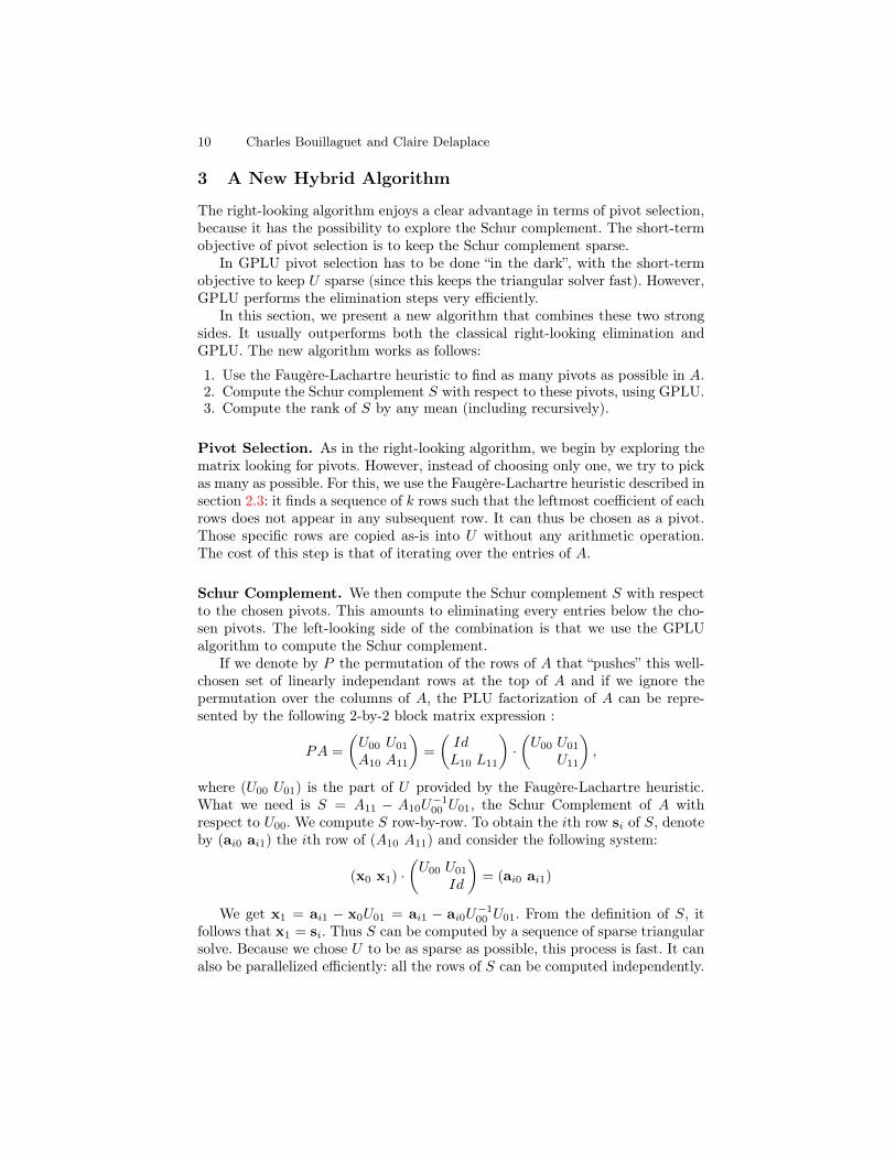
We quickly observed that no algorithm is always consistently faster than theother ; one may terminate instantly while the other may run for a long timeand vice-versa. In order to perform a systematic comparison, we decided to setan arbitrary threshold of 60 seconds, and count the number of matrices thatcould be processed in this much time. LinBox could dispatch 579 matrices, whileSpaSM processed 606. Amongst these, 568 matrices could be dealt with by bothalgorithms in less than 60s. This took 1100s to LinBox and 463s to SpaSM. LinBoxwas faster 112 times, and SpaSM 456 times. These matrices are “easy” for bothalgorithms, and thus we will not consider them anymore.

Table 2 shows the cases where one algorithm took less than 60s while the othertook more. There are cases where each of the two algorithm is catastrophicallyslower than the other. In some cases, a bug made the LinBox test program crashwith a segmentation fault. We conclude there is no clear winner (even if GPLUis usually a bit faster. The hybrid algorithm described in section 3 outperformsboth.

Matrix Right-looking GPLU HybridFranz/47104x30144bis 39 488 1.7G5/IG5-14 0.5 70 0.4G5/IG5-15 1.6 288 1.1G5/IG5-18 29 109 8GL7d/GL7d13 11 806 0.3GL7d/GL7d24 34 276 11.6Margulies/cat_ears_4_4 3 184 0.1Margulies/flower_7_4 7.5 667 2.5Margulies/flower_8_4 37 9355 3.7Mgn/M0,6.data/M0,6-D6 45 8755 0.1Homology/ch7-8.b4 173 0.2 0.2Homology/ch7-8.b5 611 45 10.7Homology/ch7-9.b4 762 0.4 0.4Homology/ch7-9.b5 3084 8.2 3.4Homology/ch8-8.b4 1022 0.4 0.5Homology/ch8-8.b5 5160 6 2.9Homology/n4c6.b7 223 0.1 0.1Homology/n4c6.b8 441 0.2 0.2Homology/n4c6.b9 490 0.3 0.2Homology/n4c6.b10 252 0.3 0.2Homology/mk12.b4 72 9.2 1.5Homology/shar_te2.b2 94 1 0.2Kocay/Trec14 80 31 4Margulies/wheel_601 7040 4 0.3Mgn/M0,6.data/M0,6-D11 722 0.4 0.6Smooshed/olivermatrix.2 75 0.6 0.1

Table 2: Comparison of sparse elimination techniques. Times are in seconds.

Sparse Gaussian Elimination modulo p: an Update 13

A reviewer asked a comparison with GBLA [3]. This is difficult, because GBLAis tailored for matrices arising in Gröbner basis computations, and exploit theirspecific shape. For instance, they have (hopefully small) dense areas, which GBLArightly store in dense data structures. This phenomenon does not occur in ourbenchmark collection, which is ill-suited to GBLA. GBLA is nevertheless undoubt-edly more efficient on Gröbner basis matrices.

Direct Methods vs Iterative Methods. We now turn our attention to theremaining matrices of the collection, the “hard” ones. Some of these are yetunamenable to any form of elimination, because they cause too much fill-in.However, some matrices can be processed much faster by our hybrid algorithmthan by any other existing method.

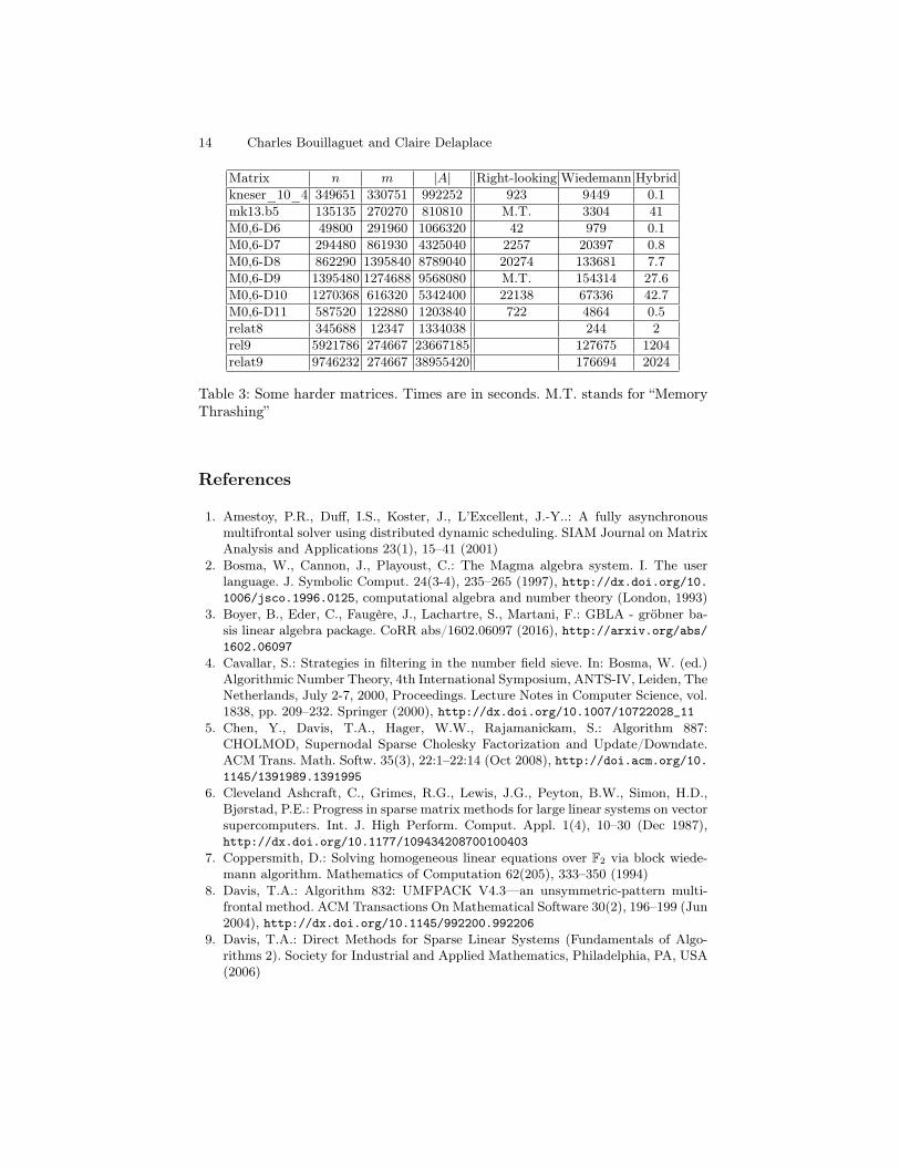
For instance, relat9 is the third largest matrix of the collection; computingits rank takes a little more than two days using the Wiedemann algorithm.Using the “Tall and Narrow Schur Complement” technique described above, thehybrid algorithm computes its rank in 34 minutes. Most of this time is spent informing a size-8937 dense matrix by computing random dense linear combinationof the 9 million remaining sparse rows. The rank of the dense matrix is quicklycomputed using the Rank function of FFLAS-FFPACK [27]. A straightforwardparallelization using OpenMP brings this down to 10 minutes using the 4 coresof our workstation (the dense rank computation is not parallel). The same goesfor the rel9 matrix, which is similar.

The rank of the M0,6-D9 matrix, which is the 9-th largest of the collection,could not be computed by the right-looking algorithm within the limit of 8GBof memory. It takes 42 hours to the Wiedemann algorithm to find its rank. Thestandard version of the hybrid algorithm finds it in less than 30 seconds.

The shar_te.b3 matrix is an interesting case. It is a very sparse matrix ofsize 200200 with only 4 non-zero entries per row. Its rank is 168310. The right-looking algorithm fails, and the Wiedemann algorithm takes 3650s. Both GPLUand the hybrid algorithm terminate in more than 5 hours. However, performingone iteration of the hybrid algorithm computes a Schur complement of size134645 with 7.4 non-zero entries per row on average. We see that the quantityn|A|, a rough indicator of the complexity of iterative methods, decreases a little.Indeed, computing the rank of the first Schur complement takes 2422s using theWiedemann algorithm. This results in a 1.5× speed-up.

All-in-all, the hybrid algorithm is capable of quickly computing the rankof the 3rd, 6th, 9th, 11th and 13th largest matrices of the collection, whereasprevious elimination techniques could not. Previously, the only possible optionwas the Wiedemann algorithm. The hybrid algorithm allows for large speedupof 100×, 1000× and 10000× in these cases.

Acknowledgement Claire Delaplace was supported by the french ANR underthe BRUTUS project. We thank the anonymous reviewers for their comments.

14 Charles Bouillaguet and Claire Delaplace

Matrix n m |A| Right-looking Wiedemann Hybridkneser_10_4 349651 330751 992252 923 9449 0.1mk13.b5 135135 270270 810810 M.T. 3304 41M0,6-D6 49800 291960 1066320 42 979 0.1M0,6-D7 294480 861930 4325040 2257 20397 0.8M0,6-D8 862290 1395840 8789040 20274 133681 7.7M0,6-D9 1395480 1274688 9568080 M.T. 154314 27.6M0,6-D10 1270368 616320 5342400 22138 67336 42.7M0,6-D11 587520 122880 1203840 722 4864 0.5relat8 345688 12347 1334038 244 2rel9 5921786 274667 23667185 127675 1204relat9 9746232 274667 38955420 176694 2024

Table 3: Some harder matrices. Times are in seconds. M.T. stands for “MemoryThrashing”

References

1. Amestoy, P.R., Duff, I.S., Koster, J., L’Excellent, J.-Y..: A fully asynchronousmultifrontal solver using distributed dynamic scheduling. SIAM Journal on MatrixAnalysis and Applications 23(1), 15–41 (2001)

2. Bosma, W., Cannon, J., Playoust, C.: The Magma algebra system. I. The userlanguage. J. Symbolic Comput. 24(3-4), 235–265 (1997), http://dx.doi.org/10.1006/jsco.1996.0125, computational algebra and number theory (London, 1993)

3. Boyer, B., Eder, C., Faugère, J., Lachartre, S., Martani, F.: GBLA - gröbner ba-sis linear algebra package. CoRR abs/1602.06097 (2016), http://arxiv.org/abs/1602.06097

4. Cavallar, S.: Strategies in filtering in the number field sieve. In: Bosma, W. (ed.)Algorithmic Number Theory, 4th International Symposium, ANTS-IV, Leiden, TheNetherlands, July 2-7, 2000, Proceedings. Lecture Notes in Computer Science, vol.1838, pp. 209–232. Springer (2000), http://dx.doi.org/10.1007/10722028_11

5. Chen, Y., Davis, T.A., Hager, W.W., Rajamanickam, S.: Algorithm 887:CHOLMOD, Supernodal Sparse Cholesky Factorization and Update/Downdate.ACM Trans. Math. Softw. 35(3), 22:1–22:14 (Oct 2008), http://doi.acm.org/10.1145/1391989.1391995

6. Cleveland Ashcraft, C., Grimes, R.G., Lewis, J.G., Peyton, B.W., Simon, H.D.,Bjørstad, P.E.: Progress in sparse matrix methods for large linear systems on vectorsupercomputers. Int. J. High Perform. Comput. Appl. 1(4), 10–30 (Dec 1987),http://dx.doi.org/10.1177/109434208700100403

7. Coppersmith, D.: Solving homogeneous linear equations over F2 via block wiede-mann algorithm. Mathematics of Computation 62(205), 333–350 (1994)

8. Davis, T.A.: Algorithm 832: UMFPACK V4.3—an unsymmetric-pattern multi-frontal method. ACM Transactions On Mathematical Software 30(2), 196–199 (Jun2004), http://dx.doi.org/10.1145/992200.992206

9. Davis, T.A.: Direct Methods for Sparse Linear Systems (Fundamentals of Algo-rithms 2). Society for Industrial and Applied Mathematics, Philadelphia, PA, USA(2006)

Sparse Gaussian Elimination modulo p: an Update 15

10. Davis, T.A., Natarajan, E.P.: Algorithm 907: KLU, A Direct Sparse Solver forCircuit Simulation Problems. ACM Trans. Math. Softw. 37(3) (2010), http://doi.acm.org/10.1145/1824801.1824814

11. Demmel, J.W., Eisenstat, S.C., Gilbert, J.R., Li, X.S., Liu, J.W.H.: A supernodalapproach to sparse partial pivoting. SIAM J. Matrix Analysis and Applications20(3), 720–755 (1999)

12. Duff, I.S., Erisman, A.M., Reid, J.K.: Direct Methods for Sparse Matrices. Numer-ical Mathematics and Scientific Computation, Oxford University Press, USA, firstpaperback edition edn. (1989)

13. Duff, I.S., Reid, J.K.: Some design features of a sparse matrix code. ACM Trans.Math. Softw. 5(1), 18–35 (Mar 1979), http://doi.acm.org/10.1145/355815.355817

14. Duff, I.S., Reid, J.K.: The multifrontal solution of indefinite sparse symmetriclinear. ACM Trans. Math. Softw. 9(3), 302–325 (Sep 1983), http://doi.acm.org/10.1145/356044.356047

15. Dumas, J.G., Villard, G.: Computing the rank of sparse matrices over finitefields. In: Ganzha, V.G., Mayr, E.W., Vorozhtsov, E.V. (eds.) CASC’2002, Pro-ceedings of the fifth International Workshop on Computer Algebra in ScientificComputing, Yalta, Ukraine. pp. 47–62. Technische Universität München, Ger-many (September 2002), http://ljk.imag.fr/membres/Jean-Guillaume.Dumas/Publications/sparseeliminationCASC2002.pdf

16. Dumas, J.-G..: Sparse integer matrices collection, http://hpac.imag.fr17. Dumas, J.-G.., Elbaz-Vincent, P., Giorgi, P., Urbanska, A.: Parallel computation

of the rank of large sparse matrices from algebraic k-theory. In: Maza, M.M., Watt,S.M. (eds.) Parallel Symbolic Computation, PASCO 2007, International Workshop,27-28 July 2007, University of Western Ontario, London, Ontario, Canada. pp. 43–52. ACM (2007), http://doi.acm.org/10.1145/1278177.1278186

18. Faugère, J.-C.., Lachartre, S.: Parallel gaussian elimination for gröbner bases com-putations in finite fields. In: Maza, M.M., Roch, J.-L.. (eds.) PASCO. pp. 89–97.ACM (2010)

19. Gilbert, J.R., Peierls, T.: Sparse partial pivoting in time proportional to arithmeticoperations. SIAM Journal on Scientific and Statistical Computing 9(5), 862–874(1988), http://dx.doi.org/10.1137/0909058

20. Kleinjung, T., Aoki, K., Franke, J., Lenstra, A.K., Thomé, E., Bos, J.W., Gaudry,P., Kruppa, A., Montgomery, P.L., Osvik, D.A., te Riele, H.J.J., Timofeev, A.,Zimmermann, P.: Factorization of a 768-bit RSA modulus. In: Rabin, T. (ed.) Ad-vances in Cryptology - CRYPTO 2010, 30th Annual Cryptology Conference, SantaBarbara, CA, USA, August 15-19, 2010. Proceedings. Lecture Notes in ComputerScience, vol. 6223, pp. 333–350. Springer (2010), http://dx.doi.org/10.1007/978-3-642-14623-7_18

21. LaMacchia, B.A., Odlyzko, A.M.: Solving large sparse linear systems over finitefields. In: Menezes, A., Vanstone, S.A. (eds.) Advances in Cryptology - CRYPTO’90, 10th Annual International Cryptology Conference, Santa Barbara, California,USA, August 11-15, 1990, Proceedings. Lecture Notes in Computer Science, vol.537, pp. 109–133. Springer (1990), http://dx.doi.org/10.1007/3-540-38424-3_8

22. Markowitz, H.M.: The elimination form of the inverse and its application to linearprogramming. Manage. Sci. 3(3), 255–269 (Apr 1957), http://dx.doi.org/10.1287/mnsc.3.3.255

16 Charles Bouillaguet and Claire Delaplace

23. May, J.P., Saunders, B.D., Wan, Z.: Efficient matrix rank computation with ap-plication to the study of strongly regular graphs. In: Wang, D. (ed.) Symbolic andAlgebraic Computation, International Symposium, ISSAC 2007, Waterloo, On-tario, Canada, July 28 - August 1, 2007, Proceedings. pp. 277–284. ACM (2007),http://doi.acm.org/10.1145/1277548.1277586

24. Saunders, B.D., Youse, B.S.: Large matrix, small rank. In: Proceedings of the 2009International Symposium on Symbolic and Algebraic Computation. pp. 317–324.ISSAC ’09, ACM, New York, NY, USA (2009), http://doi.acm.org/10.1145/1576702.1576746

25. Saunders, D.: Matrices with two nonzero entries per row. In: Proceedings of the2015 ACM on International Symposium on Symbolic and Algebraic Computation.pp. 323–330. ISSAC ’15, ACM, New York, NY, USA (2015), http://doi.acm.org/10.1145/2755996.2756679

26. The CADO-NFS Development Team: CADO-NFS, an implementation of thenumber field sieve algorithm (2015), http://cado-nfs.gforge.inria.fr/, release2.2.0

27. The FFLAS-FFPACK group: FFLAS-FFPACK: Finite Field Linear Alge-bra Subroutines / Package, v2.0.0 edn. (2014), http://linalg.org/projects/fflas-ffpack

28. The Sage Developers: Sage Mathematics Software (Version 5.7) (2013),http://www.sagemath.org

29. Wiedemann, D.H.: Solving sparse linear equations over finite fields. IEEE Trans.Information Theory 32(1), 54–62 (1986), http://dx.doi.org/10.1109/TIT.1986.1057137