GRAHAM: SPARSE 3D CNNS 1

Sparse 3D convolutional neural networksBen Grahamb.graham@warwick.ac.uk

Department of StatisticsUniversity of WarwickCV4 7AL, UK

Abstract

We have implemented a convolutional neural network designed for processing sparsethree-dimensional input data. The world we live in is three dimensional so there are alarge number of potential applications including 3D object recognition and analysis ofspace-time objects. In the quest for efficiency, we experiment with CNNs on the 2Dtriangular-lattice and 3D tetrahedral-lattice.

1 Convolutional neural networksConvolutional neural networks (CNNs) are powerful tools for understanding data with spatialstructure such as photos. They are most commonly used in two dimensions, but they can alsobe applied more generally. One-dimensional CNNs are used for processing time-series suchas human speech [9]. Three dimensional CNNs have been used to analyze movement in 2+1dimensional space-time[5, 6] and for helping drones find a safe place to land [12]. Threedimensional convolutional deep belief networks have been used to recognize objects in 2.5Ddepth maps [15].

In [3], a sparse two-dimensional CNN is implemented to perform Chinese handwritingrecognition. When a handwritten character is rendered at moderately high resolution on atwo dimensional grid, it looks like a sparse matrix. If we only calculate the hidden units ofthe CNN that can actually see some part of the input field the pen has visited, the workloaddecreases. We have extended this idea to implement sparse 3D CNNs 1. Moving from twoto three dimensions, the curse of dimensionality becomes relevant—an N×N×N cubic gridcontains many more points than an N×N square grid. However, the curse can also be takento mean that the higher the dimension, the more likely interesting input data is to be sparse.

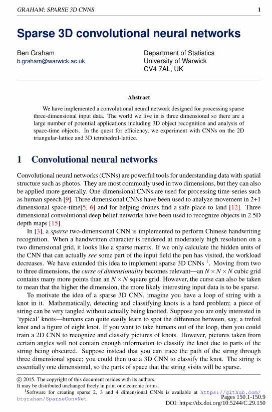
To motivate the idea of a sparse 3D CNN, imagine you have a loop of string with aknot in it. Mathematically, detecting and classifying knots is a hard problem; a piece ofstring can be very tangled without actually being knotted. Suppose you are only interested in‘typical’ knots—humans can quite easily learn to spot the difference between, say, a trefoilknot and a figure of eight knot. If you want to take humans out of the loop, then you couldtrain a 2D CNN to recognize and classify pictures of knots. However, pictures taken fromcertain angles will not contain enough information to classify the knot due to parts of thestring being obscured. Suppose instead that you can trace the path of the string throughthree dimensional space; you could then use a 3D CNN to classify the knot. The string isessentially one dimensional, so the parts of space that the string visits will be sparse.

c© 2015. The copyright of this document resides with its authors.It may be distributed unchanged freely in print or electronic forms.

1Software for creating sparse 2, 3 and 4 dimensional CNNs is available at https://github.com/btgraham/SparseConvNet Pages 150.1-150.9

DOI: https://dx.doi.org/10.5244/C.29.150

2 GRAHAM: SPARSE 3D CNNS

Figure 1: Left to right: A trefoil knot has been drawn in the cubic lattice; these are the inputlayer’s active sites. Applying a 2× 2× 2 convolution, the number of active (i.e. non-zero)sites increases. Applying a 2× 2× 2 pooling operation reduces the scale, which tends todecrease the number of active sites.

The example of the string is just a thought experiment. However, there are many real-world problems, in domains such as robotics and biochemistry, where understanding 3Dstructure is important and where sparsity is applicable.

1.1 Adding a dimension to 2D CNNs?Recently there has been an explosion of research into conventional two-dimensional CNNs.This has gone hand-in-hand with a substantial increase in available computing power thanksto GPU computing. For photographs of size 224× 224, evaluating model C of [4]’s 19convolutional layers requires 53 billion multiply-accumulate operations.

Although model C’s input is represented as a 3D array of size 224× 224× 3, it is stillfundamentally 2D—we can think of it as a 2D array of vectors, with each vector storing anRGB-color value. Model C’s initial convolutional layer consists of 96 convolutional filtersof size 7×7, applied with stride 2. Each filter is therefore applied (224/2)2 times.

This makes 3D CNNs sound like a terrible idea. Consider adapting model C’s networkarchitecture to accept 3D input with size 224× 224× 224× 3, i.e. some kind of 3D modelwhere each points has a color. To apply a 7×7×7 convolutional filter with the same stride,we would need to apply it 112 more times than in the 2D case, with each application requiring7 times as many operations. Extending the whole of model C to 3D would increase thecomputational complexity to 6.1 trillion operations. Clearly if we want to use 3D CNNs,then we need to do some things differently.

Applying the convolutions in Fourier space [11], or using separable filters [13] couldhelp, but simply the amount of memory needed to store large 3D grids of vectors wouldstill be a problem. Instead we try two things that work well together. Firstly we use muchsmaller filters, using network architectures similar to the ones introduced in [1]. The smallestnon-trivial filter possible on a cubic lattice has size 2× 2× 2, covering 23 = 8 input sites.In an attempt to improve efficiency, we will also consider the tetrahedral lattice, where thesmallest filter is a tetrahedron of size 2 which covers just 4 input sites. Secondly, we willonly consider problems where the input is sparse. This saves us from having to have theconvolutional filters visit each spatial location. If the interesting part of the input is a 1Dcurve or a 2D surface, then the majority of the 3D input field will receive only zero-vectorsfor inputs. Sparse CNNs are more efficient when used with smaller filters, as the hidden

GRAHAM: SPARSE 3D CNNS 3

(i) (ii) (iii) (iv)

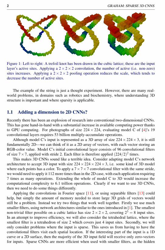
Figure 2: Convolutional filter shapes for different lattices: (i) A 4×4 square grid with a 2×2convolutional filter. (ii) A triangular grid with size 4, and a triangular filter with size 2. (iii)A 3×3×3 cubic grid, and a 2×2×2 filter. (iv) A tetrahedral grid with size 3, and a filterof size 2.

layers tend to be sparser.

1.2 CNNs on different latticesEach layer of a CNN consists of a finite graph, with a vector of input/hidden units at each site.For regular two dimensional CNNs, the graphs are square grids. The convolutional filters aresquare-shaped too, and they move over the underlying graph with two degrees of freedom;see Figure 2 (i). Similarly, 3D CNNs are normally defined on cubic grids. The convolutionalfilters are cube-shaped, and they move with three degrees of freedom; see Figure 2 (iii).

In principle we could also build 4D CNNs on hypercubic grids, and so on. However, asthe dimension d = 2,3,4, ... increases, the size 2d of the smallest non-trivial filter is growingexponentially. In the interests of efficiency, we will also consider CNNs with a differentfamily of underlying graphs. In 2D, we can build CNNs based on triangles. For each layer,the underlying graph is a triangular grid, and the convolutional filters are triangular, movingwith two degree of freedom; see Figure 3 (ii). In 3D, we can use a tetrahedral grid andtetrahedral filters that move with three degrees of freedom; see Figure 3 (iv). We couldextend this to 4D with hypertetrahedrons, etc. In d dimensions, the smallest convolutionalfilters contain only d +1 sites, rather than exponentially many.

To describe CNN architecture on these different lattices, we will still use the common“nC f/s-MPp/s-...” notation. The n counts the number of convolutional filters, f measuresthe linear size of the filters—the number of input sites the convolutional filter covers is f 2,f 3,

( f+12

),( f+2

3

)on the square, cubic, triangular and tetrahedral lattices, respectively—and

s denotes the stride. The p measures the linear size of the max-pooling regions. The /s isomitted when s = 1 for convolutions or s = p for pooling. For example, on the tetrahedrallattice 32C2−MP3/2 means 32 filters of size 2 which cover

(2+23

)= 4 input sites, followed

by max pooling with pooling regions of size(3+2

3

)= 10, and with adjacent pooling regions

overlapping by one.

1.3 Sparse operationsSparse CNNs can be thought of as an extension of the idea of sparse matrices. If a largematrix only has small number of non-zero entries per row and per column, then it makessense to use a special data structure to store the non-zero entries and their locations; thiscan both dramatically reduce memory requirements and speed up operations such as matrix

4 GRAHAM: SPARSE 3D CNNS

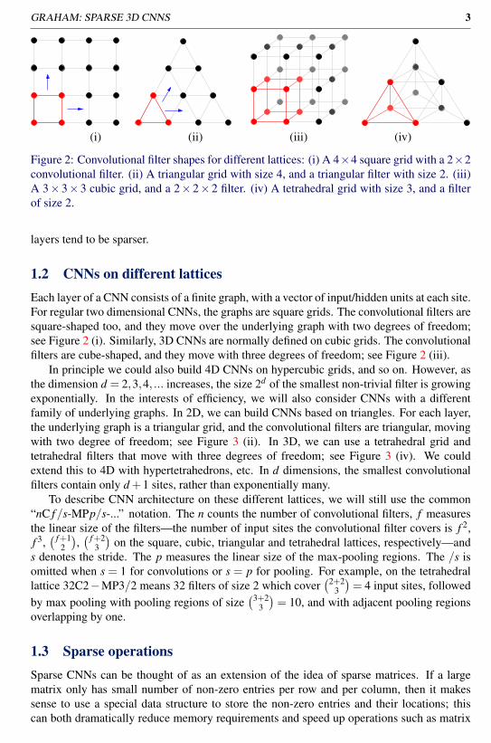
Figure 3: Calculating a 2×2 convolution for a sparse CNN: On the left is a 6×6 square gridwith 3 active sites. The convolutional filter needs to be calculated at each location that coversat least on active site; this corresponds to the shaded region. The figure on the right marksthe location of the eight active sites in the 5× 5 output layer. Sparsity decreases with eachconvolution and pooling operation. However, a CNN spends most of its time processing thelower layers, so sparsity can still be useful.

multiplication. However, if 10% of the entries are non-zero, then the advantages of sparsitymay be outweighed by the efficiency which which dense matrix multiplication can be carriedout, either using Strassen’s algorithm, or optimized GPU kernels.

The sparse CNN algorithm from [3] can be tweaked to work efficiently on general lat-tices. The spatial size of each of the CNN’s data layers is described by a lattice-type graph(similar to the ones in Figure 2). At each spatial location in the grid, there is a dimension-less vector of input or hidden units. Depending on the input, some of the spatial locationswill be defined to be active.

• A spatial location in the input layer graph is declared active if the location’s vector isnot the zero vector.

• Declare that a spatial location in a hidden layer is active if any of the spatial locationin the layer below from which it receives input are active.

See Figure 3 for a 2D example of a sparse convolution, and see Figure 1 for a 3D example.By induction, the dimension-less vectors at each non-active spatial location in the n-th

hidden layer are all the same; the shared value of the vectors can be pre-computed. We willcall this the ground state vector for the n-th level. The ground state for the input layer is justthe zero vector.

We will now describe the implementation of the sparse convolution for the types ofgraphs shown in Figure 2. For simplicity, we will focus on case (i), the 2D square grid;the other cases are very similar.

Suppose that an image has input field size min×min, and that the number of active spatiallocations is ain ∈ {0,1, . . . ,m2

in}. Suppose an f × f convolutional filter will act on the image,and let nin and nout denote the number of input and output features per spatial location. Theinput to the first convolutional operation consists of:

• A matrix Min with size ain× nin. Each row corresponds to the vector at one of theactive spatial locations.

• A map or hash table Hin of (key,value) pairs. The keys are the active spatial locations.The values record the number of the corresponding row in Min.

• The input layer’s ground state vector gin.

GRAHAM: SPARSE 3D CNNS 5

• An ( f 2nin)×nout matrix W containing the weights that define the convolution.

• A vector B of length nout specifying the values of the bias units.

To calculate the output of the first hidden layer:

1. Iterate through Hin and determine the number aout of active spatial locations in theoutput layer. A site in the output layer is active if any of the input sites are active.Build a hash table Hout to uniquely identify each of the active output spatial locationswith one of the integers 1,2, . . .aout.

2. Use Hin, Min and gin to build a matrix Q of size aout× ( f 2nin); each row of Q shouldcorrespond to the inputs visible to the convolutional filter at the corresponding outputspatial location.

3. Calculate Mout = Q×W +B.

We implemented step 1 on the CPU and steps 2 and 3 on the GPU. If W is small, the com-putational bottleneck will be I/O-related, steps 1 and 2. If W is large, the bottleneck will beperforming the dense matrix multiplication in step 3 to calculate Mout.

The procedure for max-pooling is similar. Max-pooling is always I/O-bound.

2 ExperimentsWe have performed experiments to test triangular and sparse 3D CNNs. Unlike the 2D case,there are not yet any standard benchmarks for evaluating 3D CNNs, so we just picked arange of different types of data. When faced with a trade-off between computational costand accuracy, we have preferred to train smaller network to see what can be achieved on alimited computational budget, rather than trying to maximize performance at any cost.

For some of the experiments we used n-fold repetitive testing: we processed each testcase n times, with some form of data augmentation, for n a small integer, and averaged theoutput.

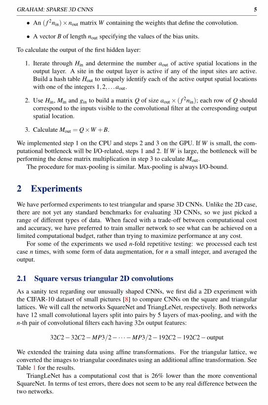
2.1 Square versus triangular 2D convolutionsAs a sanity test regarding our unusually shaped CNNs, we first did a 2D experiment withthe CIFAR-10 dataset of small pictures [8] to compare CNNs on the square and triangularlattices. We will call the networks SquareNet and TriangLeNet, respectively. Both networkshave 12 small convolutional layers split into pairs by 5 layers of max-pooling, and with then-th pair of convolutional filters each having 32n output features:

32C2−32C2−MP3/2−·· ·−MP3/2−192C2−192C2−output

We extended the training data using affine transformations. For the triangular lattice, weconverted the images to triangular coordinates using an additional affine transformation. SeeTable 1 for the results.

TriangLeNet has a computational cost that is 26% lower than the more conventionalSquareNet. In terms of test errors, there does not seem to be any real difference between thetwo networks.

6 GRAHAM: SPARSE 3D CNNS

CNN MegaOps test error 12-fold test errorSquareNet 41 9.24% 7.66%

TriangLeNet 30 9.70% 7.50%Table 1: Comparison between square and triangular 2D CNNs for CIFAR-10

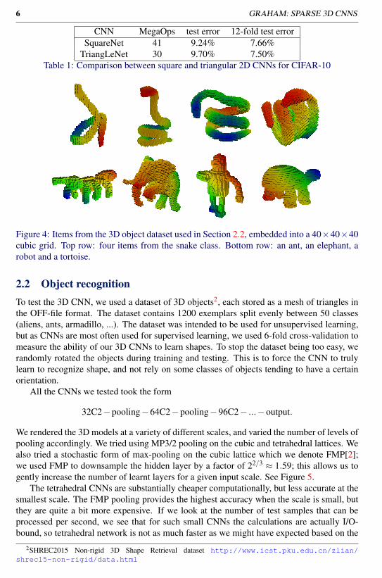
Figure 4: Items from the 3D object dataset used in Section 2.2, embedded into a 40×40×40cubic grid. Top row: four items from the snake class. Bottom row: an ant, an elephant, arobot and a tortoise.

2.2 Object recognitionTo test the 3D CNN, we used a dataset of 3D objects2, each stored as a mesh of triangles inthe OFF-file format. The dataset contains 1200 exemplars split evenly between 50 classes(aliens, ants, armadillo, ...). The dataset was intended to be used for unsupervised learning,but as CNNs are most often used for supervised learning, we used 6-fold cross-validation tomeasure the ability of our 3D CNNs to learn shapes. To stop the dataset being too easy, werandomly rotated the objects during training and testing. This is to force the CNN to trulylearn to recognize shape, and not rely on some classes of objects tending to have a certainorientation.

All the CNNs we tested took the form

32C2−pooling−64C2−pooling−96C2− ...−output.

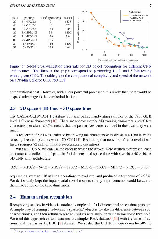
We rendered the 3D models at a variety of different scales, and varied the number of levels ofpooling accordingly. We tried using MP3/2 pooling on the cubic and tetrahedral lattices. Wealso tried a stochastic form of max-pooling on the cubic lattice which we denote FMP[2];we used FMP to downsample the hidden layer by a factor of 22/3 ≈ 1.59; this allows us togently increase the number of learnt layers for a given input scale. See Figure 5.

The tetrahedral CNNs are substantially cheaper computationally, but less accurate at thesmallest scale. The FMP pooling provides the highest accuracy when the scale is small, butthey are quite a bit more expensive. If we look at the number of test samples that can beprocessed per second, we see that for such small CNNs the calculations are actually I/O-bound, so tetrahedral network is not as much faster as we might have expected based on the

2SHREC2015 Non-rigid 3D Shape Retrieval dataset http://www.icst.pku.edu.cn/zlian/shrec15-non-rigid/data.html

GRAHAM: SPARSE 3D CNNS 7

scale pooling ×106 operations tests/s20 4×MP3/24 9 113340 5×MP3/24 35 67580 6×MP3/24 143 28620 4×MP3/2 � 36 119040 5×MP3/2 � 126 79480 6×MP3/2 � 406 31020 6×FMP� 116 110032 7×FMP� 279 849

02

46

8

Computational cost, millions of operations

Cro

ss v

alid

atio

n er

rror

, %

10 30 100 300 1000

●

●

●

20

●●

●

40

●

● ●80

●

●

●

20

●

●●

40●

● ●80

●

● ●

20

●●

●

32

Architecture

Tetrahedral MP3/2Cubic MP3/2Cubic FMP

Figure 5: 6-fold cross-validation error rate for 3D object recognition for different CNNarchitectures. The lines in the graph correspond to performing 1-, 2- and 3-fold testingwith a given CNN. The table given the computational complexity and speed of the networkon a Nvidia GeForce GTX 780 GPU.

computational cost. However, with a less powerful processor, it is likely that there would bea speed advantage to the tetrahedral lattice.

2.3 2D space + 1D time = 3D space-time

The CASIA-OLHWDB1.1 database contains online handwriting samples of the 3755 GBKlevel-1 Chinese characters [10]. There are approximately 240 training characters, and 60 testcharacters, per class. Online means that the pen strokes were recorded in the order they weremade.

A test error of 5.61% is achieved by drawing the characters with size 40×40 and learningto recognize their pictures with a 2D CNN [1]. Evaluating that network’s four convolutionallayers requires 72 million multiply-accumulate operations.

With a 3D CNN, we can use the order in which the strokes were written to represent eachcharacter as a collection of paths in 2+1 dimensional space-time with size 40× 40× 40. A3D CNN with architecture

32C3−MP3/2−64C2−MP3/2−128C2−MP3/2−256C2−MP3/2−512C3−output

requires on average 118 million operations to evaluate, and produced a test error of 4.93%.We deliberately kept the input spatial size the same, so any improvements would be due tothe introduction of the time dimension.

2.4 Human action recognition

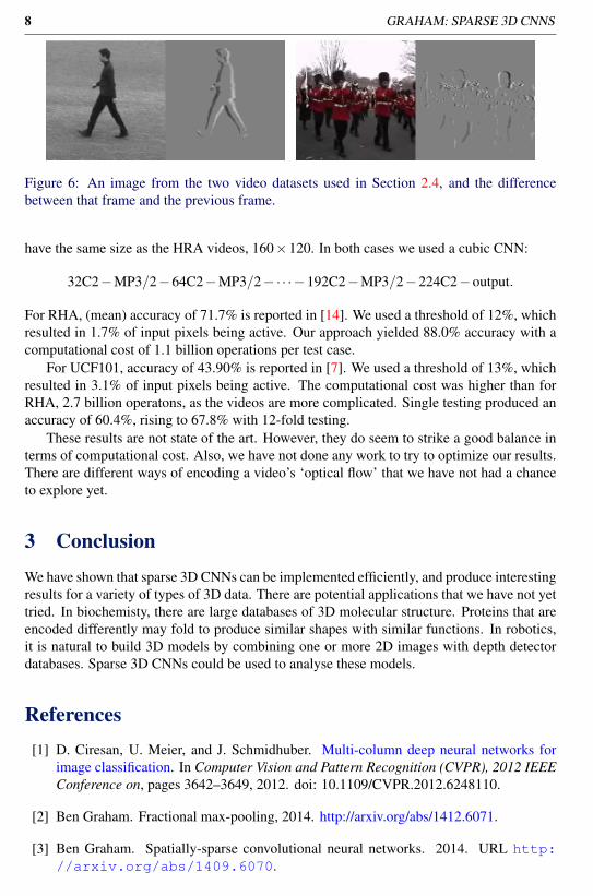
Recognizing actions in videos is another example of a 2+1 dimensional space-time problem.A simple way of turning a video into a sparse 3D object is to take the difference between suc-cessive frames, and then setting to zero any values with absolute value below some threshold.We tried this approach on two datasets, the simpler RHA dataset3 [14] with 6 classes of ac-tions, and the harder UCF101 [7] dataset. We scaled the UCF101 video down by 50% to

3http://www.nada.kth.se/cvap/actions/

8 GRAHAM: SPARSE 3D CNNS

Figure 6: An image from the two video datasets used in Section 2.4, and the differencebetween that frame and the previous frame.

have the same size as the HRA videos, 160×120. In both cases we used a cubic CNN:

32C2−MP3/2−64C2−MP3/2−·· ·−192C2−MP3/2−224C2−output.

For RHA, (mean) accuracy of 71.7% is reported in [14]. We used a threshold of 12%, whichresulted in 1.7% of input pixels being active. Our approach yielded 88.0% accuracy with acomputational cost of 1.1 billion operations per test case.

For UCF101, accuracy of 43.90% is reported in [7]. We used a threshold of 13%, whichresulted in 3.1% of input pixels being active. The computational cost was higher than forRHA, 2.7 billion operatons, as the videos are more complicated. Single testing produced anaccuracy of 60.4%, rising to 67.8% with 12-fold testing.

These results are not state of the art. However, they do seem to strike a good balance interms of computational cost. Also, we have not done any work to try to optimize our results.There are different ways of encoding a video’s ‘optical flow’ that we have not had a chanceto explore yet.

3 ConclusionWe have shown that sparse 3D CNNs can be implemented efficiently, and produce interestingresults for a variety of types of 3D data. There are potential applications that we have not yettried. In biochemisty, there are large databases of 3D molecular structure. Proteins that areencoded differently may fold to produce similar shapes with similar functions. In robotics,it is natural to build 3D models by combining one or more 2D images with depth detectordatabases. Sparse 3D CNNs could be used to analyse these models.

References[1] D. Ciresan, U. Meier, and J. Schmidhuber. Multi-column deep neural networks for

image classification. In Computer Vision and Pattern Recognition (CVPR), 2012 IEEEConference on, pages 3642–3649, 2012. doi: 10.1109/CVPR.2012.6248110.

[2] Ben Graham. Fractional max-pooling, 2014. http://arxiv.org/abs/1412.6071.

[3] Ben Graham. Spatially-sparse convolutional neural networks. 2014. URL http://arxiv.org/abs/1409.6070.

GRAHAM: SPARSE 3D CNNS 9

[4] Kaiming He, Xiangyu Zhang, Shaoqing Ren, and Jian Sun. Delving deep intorectifiers: Surpassing human-level performance on imagenet classification, 2014.http://arxiv.org/abs/1502.01852.

[5] Shuiwang Ji, Wei Xu, Ming Yang, and Kai Yu. 3d convolutional neural networksfor human action recognition. IEEE Trans. Pattern Anal. Mach. Intell., 35(1):221–231, January 2013. ISSN 0162-8828. doi: 10.1109/TPAMI.2012.59. URL http://dx.doi.org/10.1109/TPAMI.2012.59.

[6] Andrej Karpathy, George Toderici, Sanketh Shetty, Thomas Leung, Rahul Sukthankar,and Li Fei-Fei. Large-scale video classification with convolutional neural networks. InCVPR, 2014.

[7] Amir Roshan Zamir Khurram Soomro and Mubarak Shah. UCF101: A dataset of101 human action classes from videos in the wild. Technical report, November 2012.CRCV-TR-12-01.

[8] Alex Krizhevsky. Learning Multiple Layers of Features from Tiny Images. Technicalreport, 2009.

[9] Y. LeCun and Y. Bengio. Convolutional networks for images, speech, and time-series.In M. A. Arbib, editor, The Handbook of Brain Theory and Neural Networks. MITPress, 1995.

[10] C.-L. Liu, F. Yin, D.-H. Wang, and Q.-F. Wang. CASIA online and of-fline Chinese handwriting databases. In Proc. 11th International Conferenceon Document Analysis and Recognition (ICDAR), Beijing, China, pages 37–41, 2011. URL http://www.nlpr.ia.ac.cn/databases/download/ICDAR2011-CASIA%20databases.pdf.

[11] Michael Mathieu, Mikael Henaff, and Yann LeCun. Fast training of convolutionalnetworks through ffts. In International Conference on Learning Representations(ICLR2014). CBLS, April 2014. URL http://openreview.net/document/aa6ab717-ca19-47e1-a958-823b9a106ca9.

[12] D. Maturana and S. Scherer. 3D Convolutional Neural Networks for Landing ZoneDetection from LiDAR. In ICRA, 2015.

[13] Roberto Rigamonti, Amos Sironi, Vincent Lepetit, and Pascal Fua. Learning separablefilters. In Computer Vision and Pattern Recognition (CVPR), 2013 IEEE Conferenceon, 2013.

[14] Christian Schuldt, Ivan Laptev, and Barbara Caputo. Recognizing human actions:A Local SVM approach, 2004. URL http://dx.doi.org/10.1109/ICPR.2004.747.

[15] Zhirong Wu, Shuran Song, Aditya Khosla, Fisher Yu, Linguang Zhang, Xiaoou Tang,and Jianxiong Xiao. 3d shapenets: A deep representation for volumetric shapes. In TheIEEE Conference on Computer Vision and Pattern Recognition (CVPR), June 2015.