Embed Size (px)
Citation preview
SPARES AND REPAIRSFOR MAINTAINING
REDUNDANT SYSTEMS
Karin Sandra de Smidt-Destombes
This thesis is number D-90 of the thesis series of the Beta Research School for Operations
Management and Logistics. The Beta Research School is a joint effort of the departments
of Technology Management, and Mathematics and Computer Science at the Technische
Universiteit Eindhoven and the Centre for Telematics and Information Technology at the
University of Twente. Beta is the largest research centre in the Netherlands in the field of
operations management in technology-intensive environments. The mission of Beta is to
carry out fundamental and applied research on the analysis, design and control of opera-
tional processes.
This work was partly carried out at the Netherlands Organisation for Applied Scientific
Research TNO. TNO partially supported the publication costs of this dissertation.
ISBN 90-365-2400-8
c° K.S. de Smidt - Destombes, Nootdorp 2006
Printed by TNO, The Hague, The Netherlands
SPARES AND REPAIRSFOR MAINTAINING
REDUNDANT SYSTEMS
PROEFSCHRIFT
ter verkrijging van
de graad van doctor aan de Universiteit Twente,
op gezag van de rector magnificus,
prof. dr. W.H.M. Zijm,
volgens besluit van het College voor Promoties
in het openbaar te verdedigen
op vrijdag 27 oktober 2006 om 16.45 uur
door
Karin Sandra de Smidt-Destombes
geboren op 15 juni 1974
te Alkmaar

Dit proefschrift is goedgekeurd door de promotor:
Prof. dr. A. van Harten
en de assistent-promotor:
Dr. M.C. van der Heijden
Acknowledgements
It all started in 1999 when the research institute TNO asked me if it was possible
to find expressions for the availability and reliability of a system depending on the system
logistics. After some discussions with my colleagues on the subject I drew the conclusion
that this issue could not be solved within the limited amount of time available. The subject
however interested me enough that I started thinking of a way to extend my research hours
substantially. Then, I raised the idea of performing a PhD research to my manager Martin
van Dongen. Martin and René Willems showed enough confidence in me to give me the
opportunity and so in the year 2000, I started my research for two days a week.
At the University of Twente a promotor was found in the person of Henk Zijm.
However in September 2002, due to lack of time, the promotorship was handed over to Aart
van Harten and Matthieu van der Heijden. At the same time I started doing my research
physically at the University of Twente in close cooperation with Matthieu. This gave the
research a real impulse. I proceeded for two and a half years after which I finished the
research and started writing my thesis during and after my pregnancy.
Altogether, the years 2000 until 2006 have been very hectic with a lot of work,
travelling and very little spare time. This, I could not have done without the support of
the many people surrounding me. Especially Aart who was willing to be my promotor and
Matthieu who invested so much time and effort. From TNO my special thanks are for Ana
Barros and Kurt Koevoets who were always there to stimulate me and to try and find some
extra time for my research.
Maybe less visible, but not less important to me, was the way I was accepted as
a full member of the group Operational Methods for Production and Logistics of Aart van

iv
Harten. They gave me a very warm welcome, which made it easier for me to be away from
home so much.
Finally, I would like to thank the people that are dearest to me, my parents and
Dennis, for their constant support and their confidence in me. At times when I had trouble
to set myself to my work or I was disappointed because my model did not give the results I
was looking for they were always there for me. They helped me finish this thesis with their
stimulating words and their love for me.
Obviously, it is not possible for me to mention everyone here, but that does not
mean I appreciate their input any less.
Karin de Smidt - Destombes
Nootdorp, June 2006
Contents
Acknowledgements iii
1 Introduction 11.1 Research motivation . . . . . . . . . . . . . . . . . . . . . . . . . . . . . . . 11.2 Research design . . . . . . . . . . . . . . . . . . . . . . . . . . . . . . . . . . 4
1.2.1 Problem definition and research objective . . . . . . . . . . . . . . . 41.2.2 Scope . . . . . . . . . . . . . . . . . . . . . . . . . . . . . . . . . . . 51.2.3 Research questions and approach . . . . . . . . . . . . . . . . . . . . 51.2.4 Core concepts . . . . . . . . . . . . . . . . . . . . . . . . . . . . . . . 8
1.3 Literature . . . . . . . . . . . . . . . . . . . . . . . . . . . . . . . . . . . . . 141.3.1 Maintenance models . . . . . . . . . . . . . . . . . . . . . . . . . . . 141.3.2 Spare parts models . . . . . . . . . . . . . . . . . . . . . . . . . . . . 161.3.3 Interaction between maintenance and spare parts . . . . . . . . . . . 171.3.4 Interaction between maintenance and repair capacity . . . . . . . . . 181.3.5 Interaction between spare parts and repair capacity . . . . . . . . . 181.3.6 Interaction between maintenance, spares and repair capacity . . . . 19
1.4 Outline . . . . . . . . . . . . . . . . . . . . . . . . . . . . . . . . . . . . . . 20
2 Single system without wear-out 232.1 An exact algorithm . . . . . . . . . . . . . . . . . . . . . . . . . . . . . . . . 26
2.1.1 Zero lead-time (L = 0) . . . . . . . . . . . . . . . . . . . . . . . . . . 262.1.2 Positive lead-time (L > 0) . . . . . . . . . . . . . . . . . . . . . . . . 31
2.2 An approximation . . . . . . . . . . . . . . . . . . . . . . . . . . . . . . . . 342.3 Numerical results . . . . . . . . . . . . . . . . . . . . . . . . . . . . . . . . . 37
2.3.1 Exact and approximate analysis for a 58-out-of-64 system . . . . . . 372.3.2 Approximate analysis for a 2700-out-of-3000 system . . . . . . . . . 39
2.4 Model variations . . . . . . . . . . . . . . . . . . . . . . . . . . . . . . . . . 412.4.1 Sufficient repair capacity . . . . . . . . . . . . . . . . . . . . . . . . . 412.4.2 Different repair capacities during Tm +L and during maintenance time 422.4.3 System is shut down after more than N − k component failures . . . 422.4.4 Cold stand-by redundancy . . . . . . . . . . . . . . . . . . . . . . . . 422.4.5 Including component replacement times . . . . . . . . . . . . . . . . 43
2.5 Conclusions . . . . . . . . . . . . . . . . . . . . . . . . . . . . . . . . . . . . 44
vi CONTENTS
3 Single system with wear-out 453.1 An analytical approximation . . . . . . . . . . . . . . . . . . . . . . . . . . 47
3.1.1 Operational time . . . . . . . . . . . . . . . . . . . . . . . . . . . . . 473.1.2 Expected Uptime during lead-time L . . . . . . . . . . . . . . . . . . 483.1.3 Expected maintenance duration . . . . . . . . . . . . . . . . . . . . . 493.1.4 Computational issues . . . . . . . . . . . . . . . . . . . . . . . . . . 53
3.2 An iterative approximation . . . . . . . . . . . . . . . . . . . . . . . . . . . 533.2.1 Expected uptime during lead-time L . . . . . . . . . . . . . . . . . . 533.2.2 Expected maintenance duration . . . . . . . . . . . . . . . . . . . . . 54
3.3 Numerical results . . . . . . . . . . . . . . . . . . . . . . . . . . . . . . . . . 583.4 Model variations . . . . . . . . . . . . . . . . . . . . . . . . . . . . . . . . . 62
3.4.1 Maintenance also based on degraded components . . . . . . . . . . . 623.4.2 Replacement of failed components only . . . . . . . . . . . . . . . . 633.4.3 Stochastic lead-time L . . . . . . . . . . . . . . . . . . . . . . . . . . 653.4.4 Cold stand-by redundancy . . . . . . . . . . . . . . . . . . . . . . . . 66
3.5 Conclusions . . . . . . . . . . . . . . . . . . . . . . . . . . . . . . . . . . . . 66
4 Multiple systems without wear-out 694.1 Model analysis . . . . . . . . . . . . . . . . . . . . . . . . . . . . . . . . . . 734.2 Moment iteration scheme . . . . . . . . . . . . . . . . . . . . . . . . . . . . 754.3 Large versus small number of components . . . . . . . . . . . . . . . . . . . 784.4 Numerical results . . . . . . . . . . . . . . . . . . . . . . . . . . . . . . . . . 794.5 Conclusions . . . . . . . . . . . . . . . . . . . . . . . . . . . . . . . . . . . . 83
5 Multiple systems with wear-out 855.1 Equal repair rates: μ1 = μ2 . . . . . . . . . . . . . . . . . . . . . . . . . . . 865.2 Different repair rates: μ1 6= μ2 . . . . . . . . . . . . . . . . . . . . . . . . . . 88
5.2.1 Repair strategy . . . . . . . . . . . . . . . . . . . . . . . . . . . . . . 885.2.2 Moment iteration scheme . . . . . . . . . . . . . . . . . . . . . . . . 89
5.3 Numerical results . . . . . . . . . . . . . . . . . . . . . . . . . . . . . . . . . 935.4 Conclusions . . . . . . . . . . . . . . . . . . . . . . . . . . . . . . . . . . . . 97
6 Optimisation algorithms 996.1 Introduction . . . . . . . . . . . . . . . . . . . . . . . . . . . . . . . . . . . . 996.2 Single system . . . . . . . . . . . . . . . . . . . . . . . . . . . . . . . . . . . 101
6.2.1 Marginal analysis . . . . . . . . . . . . . . . . . . . . . . . . . . . . . 1016.2.2 Drawbacks marginal analysis . . . . . . . . . . . . . . . . . . . . . . 1046.2.3 Adjusted marginal analysis . . . . . . . . . . . . . . . . . . . . . . . 1076.2.4 Numerical results . . . . . . . . . . . . . . . . . . . . . . . . . . . . . 1116.2.5 Extension to component wear-out . . . . . . . . . . . . . . . . . . . 116
6.3 Multiple systems . . . . . . . . . . . . . . . . . . . . . . . . . . . . . . . . . 1166.3.1 Adjusted marginal analysis algorithm . . . . . . . . . . . . . . . . . 1176.3.2 Results . . . . . . . . . . . . . . . . . . . . . . . . . . . . . . . . . . 1226.3.3 Extension to multiple systems with wear-out . . . . . . . . . . . . . 124
6.4 Example: the Anaconda . . . . . . . . . . . . . . . . . . . . . . . . . . . . . 124
CONTENTS vii
6.4.1 What is the Anaconda? . . . . . . . . . . . . . . . . . . . . . . . . . 1256.4.2 Current situation . . . . . . . . . . . . . . . . . . . . . . . . . . . . . 1266.4.3 Translation into input parameters . . . . . . . . . . . . . . . . . . . 1276.4.4 Results . . . . . . . . . . . . . . . . . . . . . . . . . . . . . . . . . . 130
6.5 Conclusions . . . . . . . . . . . . . . . . . . . . . . . . . . . . . . . . . . . . 132
7 Conclusions and further research 1337.1 Conclusions . . . . . . . . . . . . . . . . . . . . . . . . . . . . . . . . . . . . 1337.2 Further research . . . . . . . . . . . . . . . . . . . . . . . . . . . . . . . . . 137
A List of notation 147
Samenvatting 149
Curriculum vitae 153

viii CONTENTS
Chapter 1
Introduction
In this thesis, we examine the interaction between the maintenance frequency,
inventory of repairable spare parts and the capacity needed to repair these spare parts to
achieve high system availability levels in a cost effective way. Specifically, we focus on k-
out-of-N systems. We give the motivation for this research in Section 1.1. In Section 1.2 we
explain the research design including the research objective, research questions and research
approach. To position our research in this field we give an overview of related literature in
Section 1.3. We end this chapter, Section 1.4, with an outline for the remaining part of this
thesis.
1.1 Research motivation
Many of today’s technological systems, such as aircraft, military installations,
wafer steppers or advanced medical equipment are characterised by a high level of complex-
ity and sophistication. The users of such capital assets usually demand a high availability,
because the consequences of downtime can be serious. For example, downtime of a wafer
stepper in the semiconductor industry may cause loss of production while downtime of mili-
tary equipment during a military operation may lead to a mission failure. Availability is in-
fluenced by many decisions, both during system design (component choice, redundancy) and
during exploitation (maintenance frequency, amount of maintenance resources like service
engineers, equipment and spare parts). Because of the large number of factors influencing
both system availability and life cycle costs, the trade-off between system availability and
the costs involved is complex. A common approach is to decompose the overall trade-off in
2 Introduction
a set of subproblems. However, it is not always clear to what extent each subproblem can
be solved independently of the other subproblems.
An example of two related subproblems is the choice of maintenance frequency
on the one hand and the choice of spare parts inventories on the other. Traditionally,
these decisions are separated. Still, it can be argued that there is an interaction indeed.
Demand for spare parts arises from both preventive and corrective maintenance. Choosing
the preventive maintenance frequency partially determines the timing of the demand for
spare parts. A higher preventive maintenance frequency leads to higher maintenance cost,
but at the same time leads to a more predictable demand for spare parts and hence leads
to smaller spare part safety stocks. Therefore, it is worthwhile to examine the interaction
between spare part inventories and the maintenance frequency.
Another example is the choice of repairable spare part inventories on the one hand
and the capacity needed to repair these spare parts on the other. Although these seem to
be separate decisions, there is a clear interaction as has been noticed before in the literature
(see e.g. Sleptchenko (2002)). Low repair capacity means a high utilisation rate of the
repair shop, and therefore long spare part repair lead times. As safety stocks should cover
the demand during the lead time, this means that savings on the repair capacity lead to a
need for more spare parts and vice versa. In this thesis we study the interaction between
maintenance frequency, spare part inventories and repair capacity as described above. We
illustrate the occurrence of such interactions in practice by three examples.
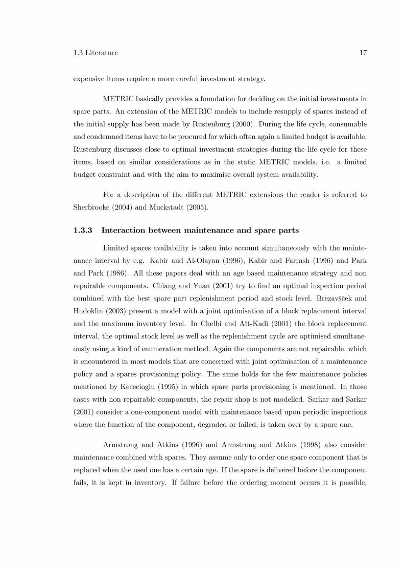
Active Phased Array Radar (APAR)
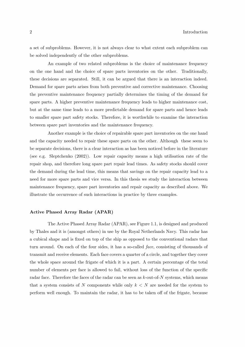
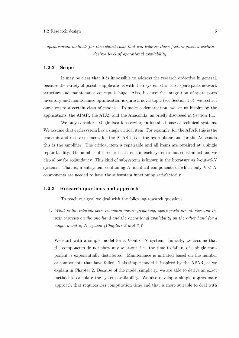
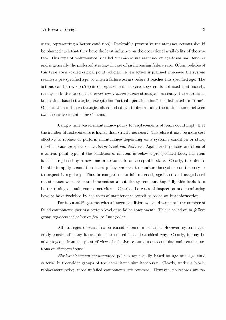
The Active Phased Array Radar (APAR), see Figure 1.1, is designed and produced
by Thales and it is (amongst others) in use by the Royal Netherlands Navy. This radar has
a cubical shape and is fixed on top of the ship as opposed to the conventional radars that
turn around. On each of the four sides, it has a so-called face, consisting of thousands of
transmit and receive elements. Each face covers a quarter of a circle, and together they cover
the whole space around the frigate of which it is a part. A certain percentage of the total
number of elements per face is allowed to fail, without loss of the function of the specific
radar face. Therefore the faces of the radar can be seen as k-out-of-N systems, which means
that a system consists of N components while only k < N are needed for the system to
perform well enough. To maintain the radar, it has to be taken off of the frigate, because
1.1 Research motivation 3
Figure 1.1: The Active Phased Array Radar (left) consists of four ’faces’, each having alarge number of elements (right). A face can be modelled as a k-out-of-N system.
repair and replacement of elements have to be done in a dust-free environment and because
of the special equipment and skills of personnel that are required. So the set-up costs for
maintenance are high. Therefore maintenance is performed periodically only and not upon
each element failure. Performing maintenance less often saves costs in terms of set-up costs.
Minimising the maintenance costs implies to do maintenance after N − k + 1 failures, soafter the system fails. This maintenance rule also implies the number of failed elements to
be high, compared to doing maintenance more often, and we therefore need to have more
spare components to limit the maintenance duration. However the spare components are
rather expensive too. Maybe, we can reduce this extra amount of spare parts by using extra
repair capacity, but this also costs money and so we have a cost trade-off. Minimising the
costs for maintenance set-ups, spare parts and repair capacity in order to achieve a certain
availability level of the APAR cannot be done by sequential optimisation. As a result, we
need explicit relations between maintenance frequency, spare part inventories and repair
capacity.
Active Towed Array Sonar (ATAS)
Another example which does not have as much components as the APAR is the
Active Towed Array Sonar (ATAS). This is a hose-like system dragged behind a frigate.
4 Introduction
It consists of several tens of hydrophones used to detect objects beneath the water surface
(such as submarines). This system is also a k-out-of-N system since not all hydrophones
need to be functioning to have the system perform satisfactorily. Just like the APAR it
is not possible to replace hydrophones on board of the frigate due to calibration activities
that need to be done together with the replacement.
Anaconda
A system similar to the ATAS is the Anaconda. The Anaconda consists of sev-
eral k-out-of-N systems within acoustic modules. Each module contains a number of hy-
drophones. Next to these hydrophones, six of the seven acoustic modules can be modelled
as k-out-of-N systems with low frequency amplifiers. The seventh module consists of a
k-out-of-N system with high frequency amplifiers. This latter k-out-of-N system of high
frequency amplifiers is considered in our case study, described in further detail in Section
6.4.1.
1.2 Research design
1.2.1 Problem definition and research objective
As stated in the previous section our research focus is on operational availability
and the key factors that influence this performance measure. We face the following problem
definition:
Although preventive maintenance optimisation is usually done separately from the spare
parts inventory optimisation and repair capacity choice, these problems are interrelated. It
is not clear how strong this relation is and which cost reduction is possible using a joint
optimisation.
Since, we do not know how strong the problems are interrelated we have to start
by gaining insight in this relationship. Then we are capable of developing a model for joint
optimisation. This leads us to the following research objective, which is:
To gain insight in the relation between maintenance frequency, spare parts inventories and
repair capacity, their joint impact on the operational availability and to develop joint
1.2 Research design 5
optimisation methods for the related costs that can balance these factors given a certain
desired level of operational availability.
1.2.2 Scope
It may be clear that it is impossible to address the research objective in general,
because the variety of possible applications with their system structure, spare parts network
structure and maintenance concept is huge. Also, because the integration of spare parts
inventory and maintenance optimisation is quite a novel topic (see Section 1.3), we restrict
ourselves to a certain class of models. To make a demarcation, we let us inspire by the
applications, the APAR, the ATAS and the Anaconda, as briefly discussed in Section 1.1.
We only consider a single location serving an installed base of technical systems.
We assume that each system has a single critical item. For example, for the APAR this is the
transmit-and-receive element, for the ATAS this is the hydrophone and for the Anaconda
this is the amplifier. The critical item is repairable and all items are repaired at a single
repair facility. The number of these critical items in each system is not constrained and we
also allow for redundancy. This kind of subsystems is known in the literature as k-out-of-N
systems. That is, a subsystem containing N identical components of which only k < N
components are needed to have the subsystem functioning satisfactorily.
1.2.3 Research questions and approach
To reach our goal we deal with the following research questions.
1. What is the relation between maintenance frequency, spare parts inventories and re-
pair capacity on the one hand and the operational availability on the other hand for a
single k-out-of-N system (Chapters 2 and 3)?
We start with a simple model for a k-out-of-N system. Initially, we assume that
the components do not show any wear-out, i.e., the time to failure of a single com-
ponent is exponentially distributed. Maintenance is initiated based on the number
of components that have failed. This simple model is inspired by the APAR, as we
explain in Chapter 2. Because of the model simplicity, we are able to derive an exact
method to calculate the system availability. We also develop a simple approximate
approach that requires less computation time and that is more suitable to deal with
6 Introduction
model extensions. We use Delphi to implement and test our algorithms. Because we
have both an exact and an approximate method, we can easily analyse the accuracy
of our approximations. We use our methods to get a basic insight in the relation
between maintenance, spare parts and repair capacity.
Next, we make a first model extension in Chapter 3 by allowing for component wear-
out, which we model as a two-phase failure process (again, inspired by the APAR).
That is, a component is either as good as new or degraded or failed. This is a serious
complication, because now we have more information on the system state that we
can use to initiate maintenance. Also, we can have two different types of components
in the repair shop (degraded and failed). Because an exact method is hard for this
extended model, we develop two approximate methods and we examine their accu-
racy by comparison to results from discrete event simulation. To this end, we build
a discrete event simulation model using the simulation software eM-Plant. We use
this model to examine the interaction between maintenance, spare parts and repair
capacity in more detail.
2. What is the relation between maintenance frequency, spare parts inventories and re-
pair capacity on the one hand and the operational availability on the other hand for
an installed base of k-out-of-N systems (Chapters 4 and 5)?
Just like we do for the single k-out-of-N system we start with a simple model for
systems consisting of components that do not show any wear-out (Chapter 4). We
assume that all systems are maintained by a single repair shop and that the spare
components available have to be shared by the different systems. Therefore, we do
not use the number of failed components to initiate maintenance as opposed to the
single k-out-of-N system, but instead we use a fixed maintenance interval. Compared
to the situation in which there is only one system we have a continuous parameter for
the maintenance frequency instead of a discrete parameter (i.e. the number of failed
components). For this model we develop an approximate method and use Delphi to
implement our algorithm. The accuracy of the algorithm is again tested by compari-
son with a discrete event simulation model built in eM-Plant.
We use a similar approach for the installed base of k-out-of-N systems with com-
ponents that are subject to wear-out, modelled as a two-phase failure process. We
1.2 Research design 7
develop two approximations, one in which the repair rates from both phases are equal,
and one in which the repair rates are allowed to be different.
3. How can we find a cost effective balance between maintenance frequencies, spare parts
inventories and repair capacity in order to achieve a target availability level (Chapter
6)?
To find a cost effective balance between the maintenance frequency, spare parts and
repair capacity we use the models from Chapters 2 until 5 and we develop optimisa-
tion algorithms.
Our first algorithm (Section 6.2) is applicable for the models described in Chap-
ters 2 and 3. The algorithm optimises simultaneously three discrete parameters, the
number of failed components to initiate maintenance, the number of spare parts and
the repair capacity. We use standard operations research techniques that are avail-
able in literature. We are able to check the accuracy of these optimisation algorithms
by performing a full enumeration and check which combination of maintenance rule,
spare parts inventory and repair capacity gives us the target availability level at the
lowest cost.
Our second algorithm (Section 6.3) is applicable for the models described in Chapters
4 and 5. This algorithm simultaneously optimises two discrete parameters (i.e. the
number of spares and the capacity) and one continuous parameter (i.e. the time in-
terval between two maintenance periods). To check the accuracy of this algorithm we
have to discretise the continuous parameter such that we can perform a full enumer-
ation again to check which parameter setting provides the target availability against
the lowest cost.
4. Which implications does the use of ours models have for a practical situation, the
Anaconda (Section 6.4.1)?
In order to test our models for applicability in practice, we use a case study. As
subject for this case study we use one of the systems of the Royal Netherlands Navy,
the Anaconda. This system is mentioned briefly before in Section 1.1 and is described
in further detail in Section 6.4.1.
8 Introduction
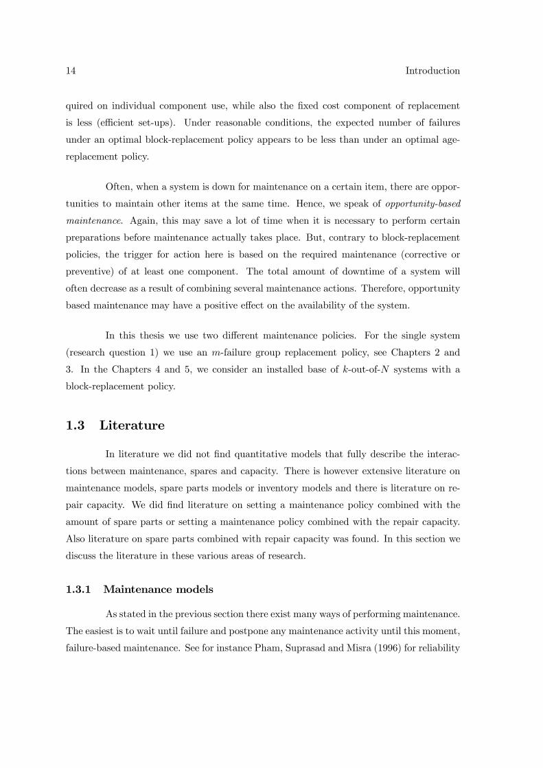
Chapter 2:
Single k-out-of-N system
no wear-out
Chapter 3:
Single k-out-of-N system
with wear-out
Chapter 4:
Multiple k-out-of-N systems
no wear-out
Chapter 5:
Multiple k-out-of-N systems
with wear-out
Chapter 6:
Optimisation method
Chapter 2:
Single k-out-of-N system
no wear-out
Chapter 3:
Single k-out-of-N system
with wear-out
Chapter 4:
Multiple k-out-of-N systems
no wear-out
Chapter 5:
Multiple k-out-of-N systems
with wear-out
Chapter 6:
Optimisation method
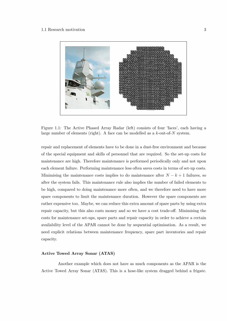
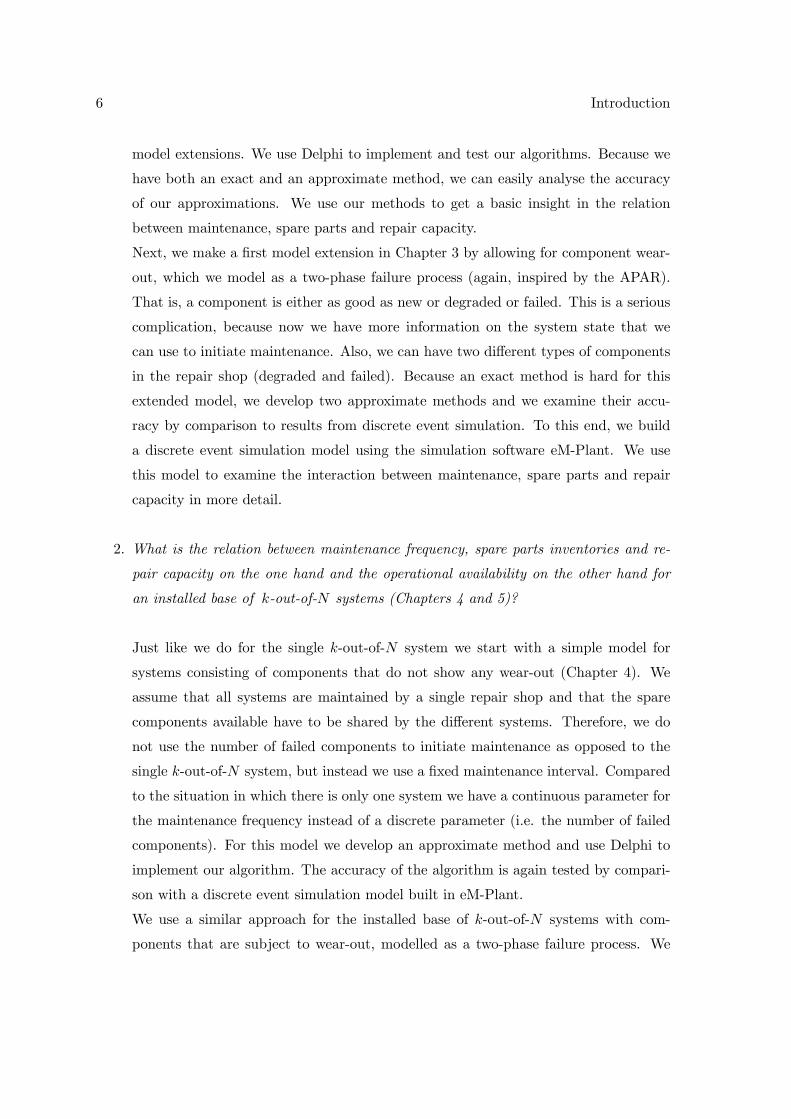
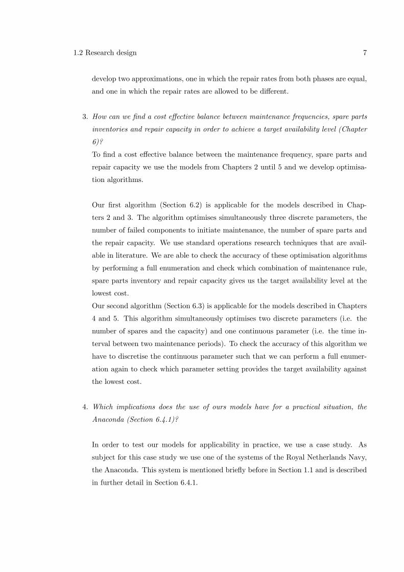
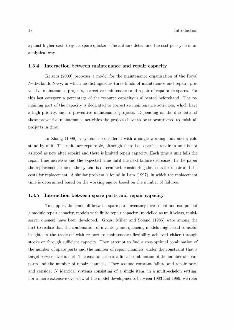
Figure 1.2: Schematic representation of the models described in each chapter.
In Figure 1.2 an schematic representation is given of the models described together
with the relevant chapters.
1.2.4 Core concepts
In our research design, we used some terminology that needs further clarification.
Because we use this terminology throughout this thesis, it is important to define what we ex-
actly mean by ”availability”, ”spare part inventories”, ”repair capacity” and ”maintenance
policy”.
Availability
In literature, various notions of availability are described. In the system design
phase, the relevant notion is the inherent availability, defined as (see Sherbrooke (2004)):
Avi =MTBF
MTBF +MTTR(1.1)
where MTBF denotes the mean time between two successive system failures and
MTTR denotes the mean time to repair the system. This performance measure refers to
1.2 Research design 9
corrective maintenance activities only and does not take into account the impact of preven-
tive maintenance activities during the exploitation phase. Therefore, a more appropriate
measure for the availability during the exploitation phase is the operational availability,
defined as (Sherbrooke (2004))
Avo =MTBM
MTBM +MDT(1.2)
where MTBM is the time between two successive maintenance activities (either
preventive or corrective) andMDT is the mean downtime. The mean time between mainte-
nance (MTBM) is generally less than the mean time between failures, because maintenance
is usually carried out to prevent system failures. The mean downtime (MDT ) can be more
or less than the mean time to repair.
On the one hand, preventive maintenance (e.g. cleaning) can take less time than
corrective maintenance. Also, downtime caused by a failure can be reduced using repair by
replacement, i.e., a failed component or module is replaced by a spare one after which the
system can be operational again whereas component repair is carried out off-line.
On the other hand, many resources (personnel, equipment, spare parts) are usually
needed for maintenance activities and waiting time occurs if one or more of the resources
needed is not immediately available.
To clarify these two effects, we can split the mean downtime MDT into two com-
ponents, the mean supply delay MSD and the mean maintenance timeMMT . Sherbrooke
(2004) refers to the mean supply delay as the waiting time for spares, because he focuses
on spare part inventory policies. However, in general the MSD may include waiting time
for other maintenance resources as well. Also, Sherbrooke (2004) decomposes the mean
maintenance time in the mean corrective maintenance time MCMT and the mean pre-
ventive maintenance time MPMT , which is correct if the MCMT (MPMT ) is the mean
corrective (preventive) maintenance time per maintenance occasion weighted with the per-
centage wc (wp)of maintenance occasions that is corrective (preventive). In other words, if
we maintain wcMCMT+wpMPMT =MMT , then we do not count any maintenance time
twice and thus our approach to characterise the MDT is correct. Hence, we can rewrite
the operational availability as
Avo =MTBM
MTBM + wcMCMT + wpMPMT +MSD(1.3)
10 Introduction
The operational availability is a crucial performance indicator during the exploita-
tion phase of capital goods. Sherbrooke (2004) argues that we can decompose the opera-
tional availability further into two components to simplify the analysis: the maintenance
availability Avmaint and the supply availability Avsupply which are defined as
Avmaint =MTBM
MTBM +wcMCMT + wpMPMT(1.4)
Avsupply =MTBM
MTBM +MSD(1.5)
If both components are close to one, the operational availability is approximately
equal to the product of the maintenance availability and the supply availability. Sherbrooke
argues that the supply availability is independent of the maintenance policy, and hence
he focuses on the supply availability for spare parts inventory optimisation. In this way,
Sherbrooke justifies that spare part inventory optimisation can be considered as a separate
sub-problem of the overall cost-availability trade-off.
In this thesis we focus on the operational availability. However, since the supply
availability is not independent of the maintenance policy, we do not split the operational
availability into maintenance availability and supply availability. If we use the shorthand
term availability in this thesis, we refer to the operational availability.
In the remainder of this section we discuss the influence of spare parts inventories,
repair capacity and maintenance policies on the supply availability and as a result also on
the operational availability as well as the interrelations.
Spare parts inventories
Spare part inventory optimisation has received a lot of interest in the scientific
literature for the following reason. Complex systems consist of many components and mod-
ules that are subject to failure and these components and modules can be very expensive.
Particularly if the installed base is geographically dispersed, this may lead to very high
spare parts inventory holding costs, because multiple stocking locations may be needed.
The objective of the spare parts inventory research is to determine how much of each spare
part (components and modules) to stock at which location in order to achieve a target
1.2 Research design 11
availability level against the lowest spare parts investment costs. This leads to multi-item,
multi-location inventory models.
For the determination of the spare parts inventories it is important to make a
distinction between repairables and consumables. Repairables are components or modules
for which it is in principle technically possible and economically useful to be repaired after
failure. A failure may of course be severe, such that repair is not possible or profitable
anymore. Consumable items however are never repaired, either because it is technically
not feasible or because it is always cheaper to buy a new one. Usually, the most expensive
spares are repairable (thousands of Euros and even up to 100.000 Euros). Therefore, a lot of
spare parts inventory research has a specific focus on repairable items and take into account
return flows and repair throughput times. Our focus in this thesis is on the repairable spare
parts in a single item and single location model.
Repair capacity
Most models for spare parts optimisation do not explicitly take into account the
repair capacity. Of course, the capacity of service engineers and equipment is an important
factor determining throughput times and work-in-process in the repair process and hence
influencing repairable spare parts inventory levels. To simplify the analysis, most models
use the assumption of an infinite capacity repair shop, which can be interpreted as ample
capacity in practice. This may be the case if a repair shop has multiple activities and
spare parts repair has high priority such that waiting time hardly occurs. Because it is not
common that waiting times are negligible, another approach is to observe repair throughput
times in practice (net repair times plus waiting time for capacity) and to use these values
as gross repair times in an infinite capacity model.
This seems to be a practical and reasonable approach at first sight, but it also has
several drawbacks. First, repair throughput times are influenced by factors as the size of
the installed base, repair shop priority settings and working methods in the repair shop.
Therefore, we cannot assume that the throughput times as observed in history remain
constant in the future, and in fact we need a separate model predicting the repair shop
throughput times. Second, there is a cost trade-off between investment in spare parts
inventories and repair capacity that infinite capacity models do not cover. If we invest in
additional repair capacity, the throughput times of the repair process decrease and therefore
12 Introduction
we need less spare parts to achieve the same supply availability. The other way around, less
investment in repair capacity leads to the need for more investment in spare parts. Note
that investment in repair capacity does not necessarily mean additional service engineers or
repair equipment, but may also include training programmes for personnel.
In this thesis, we assume finite repair capacity. We focus on capacity for the repair
of spare parts and not on the capacity for maintenance activities. Since, we consider a single
item and a single location, we are dealing with dedicated repair capacity.
Maintenance policy
Maintenance is defined as (see e.g. Blanchard (1998) and Van Dijkhuizen (1998)):
Definition 1 a series of actions to be taken with the intention to retain an item in, or
restore it to, a state in which it can perform its intended function.
There exist many ways of performing maintenance. Generally, maintenance poli-
cies consist of two procedural parts: one prescribing when to act, and the second one
prescribing what to do. Actions may involve several repair or restoration modes, or replace-
ment of the item considered. Here restoration is used for actions that bring back the item in
a better condition than the one observed before the action. The simplest maintenance pol-
icy is to wait until failure and postpone any maintenance activity until this moment. This
principle is called failure-based maintenance and does only prescribe what actions should
be taken in case of a failure. In case of a constant or decreasing failure rate, it is intuitively
clear that such a policy is the best one can do. But even in case of an increasing failure rate
such a policy may be cost effective, if breakdown costs are relatively low. A failure-based
maintenance strategy implies that the number of maintenance activities is minimal. How-
ever, when the failure of a particular item may cause consequential damage to other parts
of the system, this may lead to higher (and unexpected) capacity requirements and often
to more spare parts to replace both failed and damaged items. Under these conditions, a
preventive maintenance policy may be preferred.
The availability and reliability of a system can be increased, compared to a system
maintained according to a failure-based maintenance strategy, by performing preventive
maintenance actions. These maintenance actions will in general increase the system’s re-
liability by decreasing its actual failure rate (e.g. due to bringing the system in a better
1.2 Research design 13
state, representing a better condition). Preferably, preventive maintenance actions should
be planned such that they have the least influence on the operational availability of the sys-
tem. This type of maintenance is called time-based maintenance or age-based maintenance
and is generally the preferred strategy in case of an increasing failure rate. Often, policies of
this type are so-called critical point policies, i.e. an action is planned whenever the system
reaches a pre-specified age, or when a failure occurs before it reaches this specified age. The
actions can be revision/repair or replacement. In case a system is not used continuously,
it may be better to consider usage-based maintenance strategies. Basically, these are simi-
lar to time-based strategies, except that “actual operation time” is substituted for “time”.
Optimisation of these strategies often boils down to determining the optimal time between
two successive maintenance instants.
Using a time based-maintenance policy for replacements of items could imply that
the number of replacements is higher than strictly necessary. Therefore it may be more cost
effective to replace or perform maintenance depending on a system’s condition or state,
in which case we speak of condition-based maintenance. Again, such policies are often of
a critical point type: if the condition of an item is below a pre-specified level, this item
is either replaced by a new one or restored to an acceptable state. Clearly, in order to
be able to apply a condition-based policy, we have to monitor the system continuously or
to inspect it regularly. Thus in comparison to failure-based, age-based and usage-based
maintenance we need more information about the system, but hopefully this leads to a
better timing of maintenance activities. Clearly, the costs of inspection and monitoring
have to be outweighed by the costs of maintenance activities based on less information.
For k-out-of-N systems with a known condition we could wait until the number of
failed components passes a certain level of m failed components. This is called an m-failure
group replacement policy or failure limit policy.
All strategies discussed so far consider items in isolation. However, systems gen-
erally consist of many items, often structured in a hierarchical way. Clearly, it may be
advantageous from the point of view of effective resource use to combine maintenance ac-
tions on different items.
Block-replacement maintenance policies are usually based on age or usage time
criteria, but consider groups of the same items simultaneously. Clearly, under a block-
replacement policy more unfailed components are removed. However, no records are re-
14 Introduction
quired on individual component use, while also the fixed cost component of replacement
is less (efficient set-ups). Under reasonable conditions, the expected number of failures
under an optimal block-replacement policy appears to be less than under an optimal age-
replacement policy.
Often, when a system is down for maintenance on a certain item, there are oppor-
tunities to maintain other items at the same time. Hence, we speak of opportunity-based
maintenance. Again, this may save a lot of time when it is necessary to perform certain
preparations before maintenance actually takes place. But, contrary to block-replacement
policies, the trigger for action here is based on the required maintenance (corrective or
preventive) of at least one component. The total amount of downtime of a system will
often decrease as a result of combining several maintenance actions. Therefore, opportunity
based maintenance may have a positive effect on the availability of the system.
In this thesis we use two different maintenance policies. For the single system
(research question 1) we use an m-failure group replacement policy, see Chapters 2 and
3. In the Chapters 4 and 5, we consider an installed base of k-out-of-N systems with a
block-replacement policy.
1.3 Literature
In literature we did not find quantitative models that fully describe the interac-
tions between maintenance, spares and capacity. There is however extensive literature on
maintenance models, spare parts models or inventory models and there is literature on re-
pair capacity. We did find literature on setting a maintenance policy combined with the
amount of spare parts or setting a maintenance policy combined with the repair capacity.
Also literature on spare parts combined with repair capacity was found. In this section we
discuss the literature in these various areas of research.
1.3.1 Maintenance models
As stated in the previous section there exist many ways of performing maintenance.
The easiest is to wait until failure and postpone any maintenance activity until this moment,
failure-based maintenance. See for instance Pham, Suprasad and Misra (1996) for reliability
1.3 Literature 15
and time between successive failures predictions for k-out-of-N systems.More about the
failure-based maintenance can be found in Pintelon and Gelders (1992), Pintelon, Gelders
and Van Duyvelde (1997).
For the preventive maintenance strategies we explained in the previous section that
there are two maintenance strategies based on a time duration. The first one is the age-based
maintenance strategy, based on the calendar time, and the second one is the usage-based
maintenance strategy, based on the operation time. Optimisation of these strategies often
boils down to determining the optimal time between two successive maintenance instants;
see e.g. Van Der Duyn Schouten (1996).
For the condition-based maintenance strategy, a commonly used technique to de-
termine optimal critical points as well as optimal actions of a condition-based maintenance
policy is through the use of Markov Decision Process modelling and analysis techniques, see
e.g. Hillier and Liebermann (1995). For the so-called m-failure group replacement policy
or failure limit policy, maintenance is done after a k-out-of-N system reaches a condition
of m failed components. This maintenance policy is described by Wang (2002).
As discussed in the previous section there are not only maintenance policies based
on a single item. For instance the block-replacement policy is based on multiple items.
A comparison between age replacement of individual items, and block-replacement of the
group, has been made by Barlow and Proschan (1996). Also opportunity-based maintenance
is based on maintenance on multiple items at the same time. Van Dijkhuizen (1998) studies
a variety of models for the clustering of maintenance activities.
Maintenance models are involved with decision variables like intervals for inspec-
tion, maintenance (perfect, minimal or imperfect repair) and replacements, see e.g. Abdel-
Hameed (1995). Sometimes the action is dependent on the number of failures, like in the
model presented by Love and Guo (1996) with Weibull failure rates. Bahrami-G, Price and
Mathew (2000) present a model to determine the optimal length of the maintenance interval
for equipment that deteriorates in time.
For extensive reviews we refer to Cho and Parlar (1991) (covering the period 1976-
1988 for multi unit systems), Dekker (1996) (covering the period 1960-1996) and Dekker,
Wildeman and Duyn-Schouten (1997) (for multi component systems). For an overview of
16 Introduction
single unit and multi unit systems see Wang (2002). In Kececioglu (1995) a large amount
of maintenance strategies and variants are described.
1.3.2 Spare parts models
For the spare parts models we distinguish two kinds of models. The first kind of
models is concerned with non-repairable spare parts, also called consumables. This means
that the item is not repaired and hence is disposed of after usage. For these kind of items we
have to answer questions like when to order spare parts and how many spare parts (see e.g.
Zipkin (2000)). Especially when we could save ordering costs by ordering different items at
the same time. For these models we refer to the reviews of Osaki, Kaio and Yamada (1981)
and Kennedy, Patterson and Fredendall (2002). The second kind of models is concerned
with the repairable spare parts, which are called repairables. In this thesis, we restrict
ourselves to the second kind, the repairables.
The main stream of repairable spare parts models is based on the METRIC (Multi
Echelon Technique for Recoverable Inventory Control) theory. METRIC is a technique de-
veloped initially by Sherbrooke (1968) for applications into the US Air Force. The models
basically focus on determining optimal inventory levels for items that together determine
the optimal availability of a complex system or installation under budget constraints. The
initial models were multi-item and multi-echelon in nature but did consider only one level
of a complex product structure (single indenture models). Extensions considered multi-
indenture models and hence distinguished failures on the level of assemblies, subassemblies
or parts. This raises interesting but highly complex questions as to whether parts, sub-
assemblies or sometimes even assemblies should be kept in stock. For an extensive overview
of the history of METRIC based models, the reader is referred to Guide Jr and Srivastava
(1997) and Cho and Parlar (1991). For a more recent overview of spare parts models see
Kennedy, Patterson and Fredendall (2002).
The basic trade-off in METRIC models concerns the balancing between achieving
a target system availability and the overall investment in spares. Important in the analysis
is the system approach, instead of focussing on individual item service levels it is the contri-
bution of each item to the overall system availability that counts. A typical outcome of the
optimisation procedures is that cheap items are stocked in much larger quantities whereas
1.3 Literature 17
expensive items require a more careful investment strategy.
METRIC basically provides a foundation for deciding on the initial investments in
spare parts. An extension of the METRIC models to include resupply of spares instead of
the initial supply has been made by Rustenburg (2000). During the life cycle, consumable
and condemned items have to be procured for which often again a limited budget is available.
Rustenburg discusses close-to-optimal investment strategies during the life cycle for these
items, based on similar considerations as in the static METRIC models, i.e. a limited
budget constraint and with the aim to maximise overall system availability.
For a description of the different METRIC extensions the reader is referred to
Sherbrooke (2004) and Muckstadt (2005).
1.3.3 Interaction between maintenance and spare parts
Limited spares availability is taken into account simultaneously with the mainte-
nance interval by e.g. Kabir and Al-Olayan (1996), Kabir and Farrash (1996) and Park
and Park (1986). All these papers deal with an age based maintenance strategy and non
repairable components. Chiang and Yuan (2001) try to find an optimal inspection period
combined with the best spare part replenishment period and stock level. Brezavšcek and
Hudoklin (2003) present a model with a joint optimisation of a block replacement interval
and the maximum inventory level. In Chelbi and Aït-Kadi (2001) the block replacement
interval, the optimal stock level as well as the replenishment cycle are optimised simultane-
ously using a kind of enumeration method. Again the components are not repairable, which
is encountered in most models that are concerned with joint optimisation of a maintenance
policy and a spares provisioning policy. The same holds for the few maintenance policies
mentioned by Kececioglu (1995) in which spare parts provisioning is mentioned. In those
cases with non-repairable components, the repair shop is not modelled. Sarkar and Sarkar
(2001) consider a one-component model with maintenance based upon periodic inspections
where the function of the component, degraded or failed, is taken over by a spare one.
Armstrong and Atkins (1996) and Armstrong and Atkins (1998) also consider
maintenance combined with spares. They assume only to order one spare component that is
replaced when the used one has a certain age. If the spare is delivered before the component
fails, it is kept in inventory. If failure before the ordering moment occurs it is possible,
18 Introduction
against higher cost, to get a spare quicker. The authors determine the cost per cycle in an
analytical way.
1.3.4 Interaction between maintenance and repair capacity
Keizers (2000) proposes a model for the maintenance organisation of the Royal
Netherlands Navy, in which he distinguishes three kinds of maintenance and repair: pre-
ventive maintenance projects, corrective maintenance and repair of repairable spares. For
this last category a percentage of the resource capacity is allocated beforehand. The re-
maining part of the capacity is dedicated to corrective maintenance activities, which have
a high priority, and to preventive maintenance projects. Depending on the due dates of
these preventive maintenance activities the projects have to be subcontracted to finish all
projects in time.
In Zhang (1999) a system is considered with a single working unit and a cold
stand-by unit. The units are repairable, although there is no perfect repair (a unit is not
as good as new after repair) and there is limited repair capacity. Each time a unit fails the
repair time increases and the expected time until the next failure decreases. In the paper
the replacement time of the system is determined, considering the costs for repair and the
costs for replacement. A similar problem is found in Lam (1997), in which the replacement
time is determined based on the working age or based on the number of failures.
1.3.5 Interaction between spare parts and repair capacity
To support the trade-off between spare part inventory investment and component
/ module repair capacity, models with finite repair capacity (modelled as multi-class, multi-
server queues) have been developed. Gross, Miller and Soland (1985) were among the
first to realise that the combination of inventory and queueing models might lead to useful
insights in the trade-off with respect to maintenance flexibility achieved either through
stocks or through sufficient capacity. They attempt to find a cost-optimal combination of
the number of spare parts and the number of repair channels, under the constraint that a
target service level is met. The cost function is a linear combination of the number of spare
parts and the number of repair channels. They assume constant failure and repair rates
and consider N identical systems consisting of a single item, in a multi-echelon setting.
For a more extensive overview of the model developments between 1983 and 1989, we refer
1.3 Literature 19
to Cho and Parlar (1991). More recently Kim, Shin and Park (2000) have presented an
iterative algorithm to determine a cost optimal combination of repair capacities and spare
part levels. This model is a single item, multi echelon model as well. They claim that a
similar modelling technique can be used to tackle more complicated situations, like lateral
supply for instance.
Ebeling (1991) proposes a single echelon, multi-item model. The installed base
consists of N identical systems, each having of M different components. Each component
has its own resource capacity, which consists of at least one repair channel. Because of
these dedicated repair capacities, the model remains single item. A drawback is that the
interaction between the repairs of various components is not taken into account. Avsar and
Zijm (2003) consider more general multi-echelon resource structures in which each repair
facility may be a queueing network, and show how under Poisson failure rates stock levels at
all echelons can be optimised. A similar approach can be used for multi-indenture structures
and for combinations of multi-echelon and multi-indenture structures, see Zijm and Avsar
(2003).
In Muckstadt (2005) a model is developed to find stock levels for multiple items for
which the expected holding and backorder cost are minimised. Sleptchenko (2002) deals with
the optimisation of the number of spare parts and repair capacity in a multi-item system.
He describes what priority rules are needed in the repair shop in order to minimise the cost
investment (see Sleptchenko, Van der Heijden and Van Harten (2005)). He also shows that
repair priorities may seriously reduce the spare parts investment needed to obtain a target
supply availability. To use this model for supply availability optimisation as a component
in operational availability optimisation, a prerequisite is that component repair capacity is
not shared with maintenance capacity. If the same service engineers and/or equipment is
used for both (preventive) maintenance and component repair, the decomposition of the
availability into maintenance availability and supply availability as proposed by Sherbrooke
is not valid anymore.
1.3.6 Interaction between maintenance, spares and repair capacity
The importance of integrating the maintenance strategy with spare parts and
repair capacity has been pointed out in the literature, see for example Gross, Miller and
20 Introduction
Soland (1985) and Dinesh Kumar et al. (2000). However, only very few publications describe
quantitative models. Natarajan (1968) considers a single unit with spares and a number
of repair facilities. By determination of the time to failure the availability is determined.
Furthermore, Wang (1995), Wang and Wu (1995), Wang (1994a), Wang (1994b), Wang
(1993) consider a single system consisting of a number of operational components and
a number of stand-by components. All components are identical. Whenever one of the
components fails, a stand-by component takes over and the failed one immediately sent to a
repair shop with finite repair capacity for repair. They optimise simultaneously the number
of stand-by components, number of spares and the number of repairmen. These models are
the ones that come the closest to our problem definition. The strongest resemblance is found
in Wang (1993) in which there is a number of operating units, a number of warm stand-by
units and a number of cold stand-by units (i.e. spare units). Choosing the failure rate of
the operating and warm stand-by units to be equal, we have a redundant system in which
replacements are done after each component failure (one warm stand-by component turns
into an operating unit and a cold stand-by unit becomes warm stand-by). However, they do
not cover the interactions we consider in this thesis. They do consider a parameter affecting
the time until a system failure, namely, the number of warm stand-by units; but they do
not have a parameter for the maintenance frequency. Therefore, there is no parameter that
influences the number of maintenance set-ups (maintenance is done after every unit failure)
and as a consequence there is no parameter that affects the total maintenance costs.
To the best of our knowledge there are no books or papers that describe quanti-
tative models concerning the integration of maintenance strategy, spare parts management
and repair capacity.
1.4 Outline
The outline of this thesis is as follows. We start in Chapter 2 with the description
of a model for a single k-out-of-N system that determines the system availability for a
given maintenance strategy, a given number of spare parts and given repair capacity. In
this chapter we assume that the components have a constant failure rate. This model is
extended in Chapter 3 to a model for a single k-out-of-N system in which the components
are subject to wear-out.
1.4 Outline 21
The same is done in the Chapters 4 and 5 respectively for an installed base con-
sisting of multiple identical k-out-of-N systems without component wear-out and with com-
ponent wear-out. These systems share the same spare parts and capacity.
For each of the models from Chapters 2 till 5, we develop optimisation algorithms
in Chapter 6 so that we can find the most cost effective combination for the maintenance
strategy, number of spares and capacity without having to compute all possible combina-
tions. With these optimisation models we answer the research goal of this thesis. To show
the applicability of the models in practice we apply the model to a specific military system
called the Anaconda in Section 6.4.1.
We end this thesis with conclusions and suggestions for further research in Chapter
7.

22 Introduction
Chapter 2
Single system without wear-out
We begin this chapter1 by describing the k-out-of-N system with hot stand-by
redundancy and its maintenance process in more detail. Hot stand-by redundancy means
that all non failed components are functioning, even if this number is larger than k. So,
all components have the same failure rate. The expected number of component failures
decreases over time. Knowing the number of failed components at each moment in time
we are dealing with a condition-based maintenance strategy. The condition on which the
maintenance initiation is based is the condition of the system, the components in total, and
not the individual components.
At the start of a system uptime, all N components are as good as new. The failure
process of each component is characterised by a negative exponential distribution with rate
λ, where we assume that the component failure processes are mutually independent. The
system functions properly as long as at most N − k components have failed. To preventsystem downtime, maintenance is initiated if m ≤ N − k components have failed. It seemsreasonable to choose m = N − k if the maintenance set-up costs are high, but a lowernumber may be chosen if some lead-time L ≥ 0 is required between maintenance initiationand the actual start of maintenance activities. Looking at the naval defence systems that
motivated our research, this lead-time may be interpretted as the time needed for a ship to
come to the harbour to receive maintenance. The system is assumed to be in use during
this lead-time and it is therefore likely to degrade further.
1This chapter is based on the paper: K.S. de Smidt-Destombes, M.C. van der Heijden and A. van Harten(2004); On the availability of a k-out-of-N system given limited spares and repair capacity under a conditionbased maintenance strategy; Reliability Engineering and System Safety ; 83 (3); 287-300.
24 Single system without wear-out
The actual maintenance activities consist of replacing all failed components by
spares. However, if insufficient spares are available in an as-good-as-new condition, the
maintenance completion is delayed until sufficient failed ones have been repaired. We assume
that the components have independent and identical exponentially distributed repair times
with rate μ. The capacity for repairing components is limited and equal to c parallel
channels. For the time being, we ignore the replacement time of the components after
repair (see Section 2.4.5 for an extension in this direction). When all failed components are
replaced, the system cycle starts over again. During the time until the next maintenance
initiation (i.e., when m components have failed) plus the lead-time L, the same capacity c is
available for restoring components (see Section 2.4.2 for a generalisation to different repair
capacities during system maintenance time and non-maintenance time). It is not guaranteed
that the repair capacity is always sufficient to repair the remaining spares during the system
uptime, so the number of available spares when maintenance starts may be less than S.
Our analysis in this thesis is based on the following additional assumptions:
• The failure process of components continues during the maintenance set-up time L,even if more than N − k components have failed; the reason is that the APAR radaris always able to make partial observations in that case, so that the system will not
be shut down; we refer to Section 2.4.3 for relaxing this assumption.
• During maintenance, all failed components are replaced by new components; if it
would be optimal to replace less components (say restoring up to N1 < N), we have
in fact an k-out-of-N1 system; then, we conclude that too many components have
been included in the system design. This assumption can be relaxed in the case the
components are subject to wear-out, see Section 3.4.2.
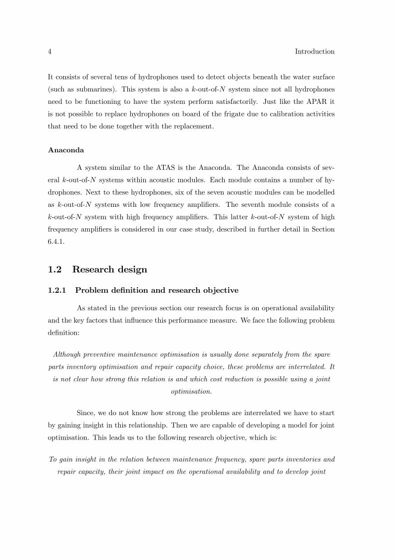
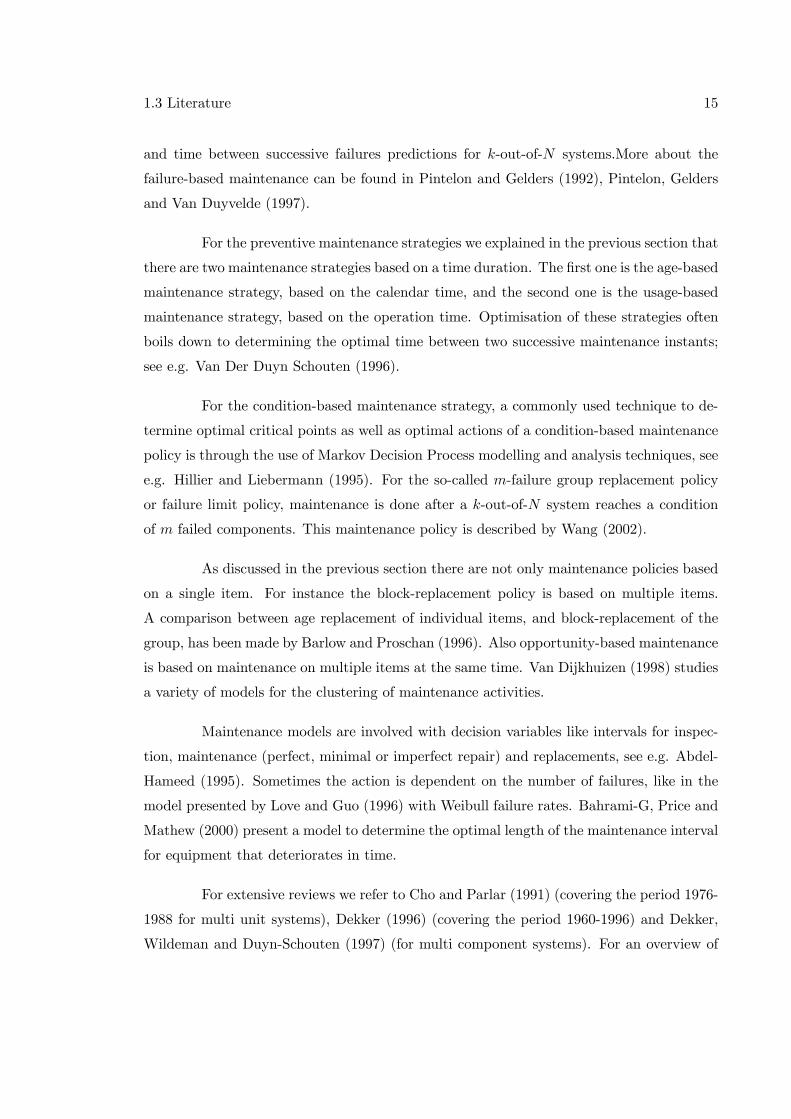
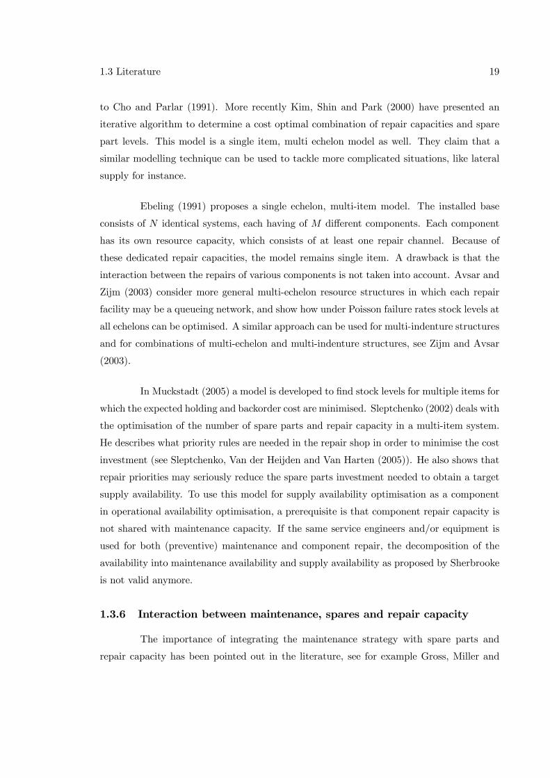
In fact, we have two interrelated cycles, namely, a cycle for the k-out-of-N system
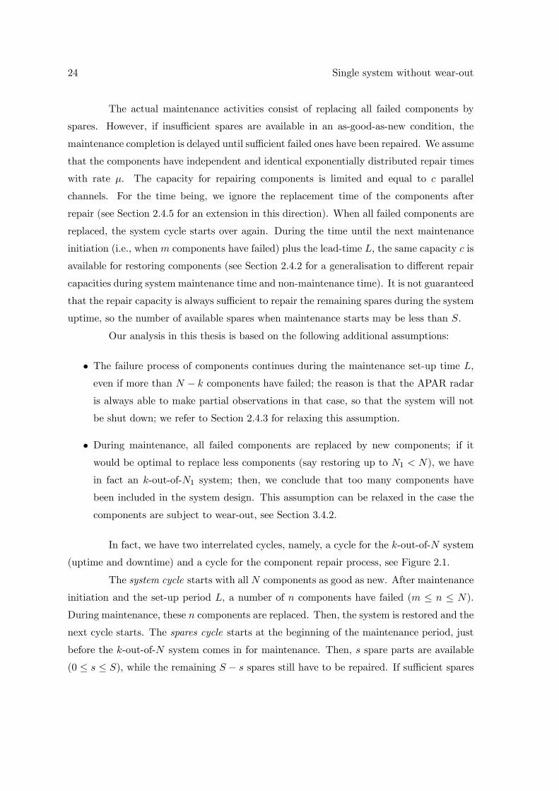
(uptime and downtime) and a cycle for the component repair process, see Figure 2.1.
The system cycle starts with all N components as good as new. After maintenance
initiation and the set-up period L, a number of n components have failed (m ≤ n ≤ N).During maintenance, these n components are replaced. Then, the system is restored and the
next cycle starts. The spares cycle starts at the beginning of the maintenance period, just
before the k-out-of-N system comes in for maintenance. Then, s spare parts are available
(0 ≤ s ≤ S), while the remaining S − s spares still have to be repaired. If sufficient spares
25
# failed comp.
# avail. spares s1
System operational System downSystem partly operational, partly down
0 m m 00
s2
n1 n2
operational time operational timeL Lmaint. maint.
# failed comp.
# avail. spares s1
System operational System downSystem partly operational, partly down
0 m m 00
s2
n1 n2
operational time operational timeL Lmaint. maint.
Figure 2.1: Interrelated cycles for a single system. The first cycle concerns the systemcomponents. The second cycle concerns the spare components.
are available (s ≥ n), all failed components are replaced and the system is operational againwithout delay. Otherwise, the system is down during the time to repair the remaining n−scomponents needed. After maintenance completion, the repair process continues until the
end of the cycle, i.e. just before the next maintenance period starts.
It is clear that the number of components at the start of a spares cycle depends
on the number of components repaired during the cycle and the number of spares to be
repaired at the start of the preceding cycle. Therefore, these cycles are interrelated. As a
solution, we will derive the steady state distribution of the number of spares s at the start of
a spares cycle. An exact steady state distribution provides us a way to an exact availability
analysis.
The operational availability equals the expected uptime during a cycle (i.e., when
at least k components are operational) divided by the expected cycle length. The expected
uptime equals the expected time until maintenance initiation E [Tm] plus the expected time
during the set-up time L that at least k components are operational E [Um]. So, we find:
AVm,S,c =E [Tm] +E [Um]
E [Tm] + L+E [Dm,S,c](2.1)
where E [Dm,S,c] is the expected maintenance time to restore the system to the new state.
Equation 2.1 implies that it is sufficient to find exact expressions for E [Tm], E [Um] and
E [Dm,S,c] as function of the three decision variables m, S and c.
We develop an exact algorithm for determining the system availability in Section
2.1 in case the lead-time is equal to zero and in case the lead-time is larger than zero.
However, it is not easy to determine the expressions needed for the availability, E [Tm],
E [Um] and E [Dm,S,c] (see equation 2.1). Therefore we also describe an approximation to
find the same system availability in Section 2.2. The results of both models are discussed in
26 Single system without wear-out
Section 2.3. We end this chapter with Section 2.4 in which some variations on the described
model are considered.
2.1 An exact algorithm
We first derive the expressions for L = 0 in Section 2.1.1, next we extend our
analysis to a positive lead-time in Section 2.1.2.
2.1.1 Zero lead-time (L = 0)
As the lead-time L = 0 we have E [U ] = 0. Hence, we only have to calculate E [Tm]
and E [Dm,S,c]. The operational time until maintenance initiation Tm can be derived by
splitting this period in the time until the first component failure, the time between the first
and the second failure, etc. The memoryless property of the exponential distribution gives
us that the time between the ith and the (i+ 1)th failure is exponentially distributed with
rate (N − i)λ. So, the expected time until the mth failure equals
E [Tm] =m−1Xi=0
1
(N − i)λ (2.2)
To derive the expected maintenance duration E [Dm,S,c], we condition on the number of
available spare parts s just before the system arrives for maintenance at the repair shop.
Then, the system downtime equals the time for restoring the m− s spares needed to repairthe system:
E [Dm,S,c] =SXs=0
E [Rc (m− s, S − s+m |s)]πm,S,c (s) (2.3)
where Rc (m− s, S − s+m |s) is the time to restorem−s spares using c servers if S−s+mcomponents are waiting to be repaired, and πm,S,c (s) is the steady state probability of
having s spares ready for use at the start of the maintenance period (just before the system
arrives), given m, S and c.
Below, we derive expressions for the two variables involved in equation 2.3. We
start with E [Rc (i, j)], where we omit the conditioning variable s since it does not contain
information and where we write i = m− s and j = S − s+m for simplicity. As obviously
E [Rc (i, j)] = 0 if i ≤ 0, we focus on the case i > 0. Then, we can determine the expectedmaintenance period analogously to the derivation of E [Tm] by splitting the period in the
2.1 An exact algorithm 27
time until the first repair completion, the time between the first and the second repair
completion, etc. We consider two situations, j ≤ c and j > c. If j ≤ c, the time to restorethe components is determined by the number of components to be restored j and not by the
repair capacity c, so the mean time until the next repair completion equals 1jμ . Otherwise,
the repair capacity is the bottleneck, and the mean time until the next repair completion
equals 1cμ . In fact, we have the recursive relation
E [Rc (i, j)] =1
min j, cμ +E [Rc (i− 1, j − 1)] (2.4)
We can elaborate this, finding the expression
E [Rc (i, j)] =
⎧⎪⎪⎪⎪⎪⎪⎪⎪⎨⎪⎪⎪⎪⎪⎪⎪⎪⎩
0 if i ≤ 0i−1Ph=0
1(j−h)μ if 0 < i ≤ j ≤ c
icμ if j > c and i ≤ j − cj−ccμ +
i−j+c−1Ph=0
1(c−h)μ if j > c and j − c < i ≤ j
(2.5)
We determine the steady state probabilities πm,S,c (s) of having s spares ready for use
at the start of the maintenance period (just before the system arrives) using a Markov
chain. Because both failure and repair times are exponentially distributed, the transition
probabilities solely depend on the state s at the beginning of a spares cycle. Each entry
(i,j) of this matrix equals the probability qi,j that j spares are available at the start of a
maintenance period while i spares were available at the start of the previous maintenance
period (i, j ∈ 0, .., S).For computational efficiency, we first aggregate all states s ≤ m in a single state
M , so the dimension of the Markov chain reduces from S+1 to S−m+1. The aggregationis useful, because we have insufficient spares available to repair the system immediately for
all s ≤ m. Therefore, the number of spares to be repaired when the new system uptime
starts equals S anyway, and so the probability of being in a specific state at the start of
the next cycle is the same for all s ≤ m. We disaggregate the aggregate state M into states
s = 0, 1, ..,m later on. Note that we have πm,S,c (M) = 1 as a special case if S < m, because
we always have insufficient spares.
We calculate the transition probabilities qi,j by conditioning on the time to main-
tenance initiation Tm = t. Given that i spares are available just before a maintenance
period starts and m spares are needed for repair, the number of spares to be repaired just
28 Single system without wear-out
after maintenance has started equals S− i+m. However, if insufficient spares are available(i < m), we have to wait until the number of spares available have increased to m, i.e. until
the number of spares to be repaired has reduced to S. Hence, the number of spares to be
repaired at the start of a system uptime equals min S, S − i+m. This number has to bereduced to S − j during the period Tm to arrive in spares state j at the start of the next
cycle. Therefore, we have
qi,j =
∞Zt=0
fm(t)Hc (min S, S − i+m , S − j, t) dt (2.6)
where fm (t) is the density function of Tm and Hc (a, b, τ) is the probability that the number
of failed spares reduces from a to b during τ , i.e. exactly a− b out of a spares are repairedduring τ with c servers. As j = M represents the aggregate state 0, ..,m, Hc (a, S −M, τ)equals the probability that at most a−S+m out of a spares are repaired during τ . Because
the number of component failures during t has a binominal distribution with parameters N
and 1− e−λt, we can derive that the density function fm (t) can be written as:
fm (t) =
µN
m− 1
¶(N − (m− 1))λe−(N−(m−1))λt
³1− e−λt
´m−1(2.7)
Regarding Hc (a, b, τ), we first note that only a positive number of components can be re-
stored during τ , so that Hc (a, b, τ) = 0 if b > a. If a = b, no components have been restored
during τ . As the repair rate equals min b, cμ, we have that Hc (b, b, t) = e−minb,cμt. Forb < a. we distinguish two cases: a ≤ c (all failed components are being repaired imme-diately) and a > c (c repairs are started initially). In the first case, the number of failed
items remaining after a period t is binomially distributed with parameters a and e−μt. In
the second case, the number of spares to repair exceeds c and only c spares can be repaired
simultaneously. We derive Hc (a, b, t) as follows. Let τ be the time at which the first repair
is completed. In the remaining time t− τ , a− 1− b out of i− 1 failed components have tobe repaired. Hence,
Hc (a, b, t) =
tZτ=0
cμe−cμτHc (a− 1, b, t− τ) dτ (2.8)
We distinguish two situations, b < c and b ≥ c. In the first situation, we start withHc (c+ 1, b, t):
2.1 An exact algorithm 29
Hc (c+ 1, b, t) =
tZτ=0
cμe−cμτHc (c, b, t− τ) dτ (2.9)
=
tZτ=0
cμe−cμτµc
b
¶e−bμ(t−τ)
³1− e−μ(t−τ)
´c−bdτ
=c−bXi=0
µc
b
¶µc− bi
¶(−1)i cμe−(b+i)μτ
tZτ=0
e−(c−b−i)μτdτ
=c−b−1Xi=0
"µc
b
¶µc− bi
¶(−1)i
cμe−(b+i)μτ¡1− e−(c−b−i)μt
¢(c− b− i)μ
#
+
µc
b
¶(−1)c−b cμte−cμt
=c−b−1Xi=0
"µc
b
¶µc− bi
¶(−1)i
c¡e−(b+i)μτ − e−cμt
¢c− b− i
#+
µc
b
¶(−1)c−b cμte−cμt
This way, we can calculate Hc (a, b, t) recursively for a = c+2, a = c+3 etcetera.
If c ≤ b < a we start with a = b+ 1:
Hc (b+ 1, b, t) =
tZτ=0
cμe−cμτHc (b, b, t− τ) dτ =
tZτ=0
cμe−cμτe−cμ(t−τ)dτ = cμte−cμt (2.10)
Again, we can calculate Hc (a, b, t) recursively for a = b + 2, a = b + 3 etcetera
resulting in:
Hc (a, b, t) =(cμt)a−b
(i− j)! e−cμt (2.11)
30 Single system without wear-out
Combining it all together, we find that:
Hc (a, b, t)
=
⎧⎪⎪⎪⎪⎪⎪⎪⎪⎪⎪⎪⎪⎪⎪⎪⎪⎪⎨⎪⎪⎪⎪⎪⎪⎪⎪⎪⎪⎪⎪⎪⎪⎪⎪⎪⎩
0a < b ∨a, b < 0
e−minb,cμt a = b¡ab
¢e−bμt
¡1− e−μt
¢a−bb ≤ a ≤ c¡
cminb,c
¢ (−1)c−minb,c(cμt)a−maxb,c(a−maxb,c)! e−cμt
+c−b−1Pg=0
¡cb
¢¡c−bg
¢(−1)g
µ³c
c−b−g
´a−c ¡e−(b+g)μt − e−cμt
¢−a−c−1Ph=1
ca−c
(c−b−g)h(μt)a−c−h
(a−c−h)! e−cμt
¶ b ≤ a∧ a > c
(2.12)
Using equations 2.7 and 2.12, we can find an explicit (but complicated) expression for the
transition probabilities qi,j as defined by equation 2.6.
Next, we have to derive the steady state probabilities πm,S,c (i) for the states
0 ≤ i ≤ m. We can use the following set of equations to derive these probabilities from the
steady state probabilities πm,S,c (i), m+ 1 ≤ i ≤ S and πm,S,c (M) for the aggregate state
representing the states 0 ≤ i ≤ m:
πm,S,c (i) = πm,S,c (M) qM,i +SP
j=m+1πm,S,c (j) qj,i if 0 ≤ i ≤ m (2.13)
For the transition probabilities qM,i, we use the fact that S spares have to be repaired at
the start of a system uptime if the spares state at the start of the cycle was s ≤ m, nomatter what the exact value of s was:
qM,i =
∞Zt=0
fm (t)Hc (S, S − i, t) dt (2.14)
Note that, as usual in Markov chains, we have a dependent system of equations, which
we can solve by replacing one arbitrary equation by the condition that the entries of the
vector πm,S,c (i) add up to one. We can solve this system of equations using any standard
numerical procedure, see e.g. Press [2002].
Combining all stationary probabilities πm,S,c(s) with equation 2.5 we findE [Dm,S,c]
from equation 2.3.
2.1 An exact algorithm 31
2.1.2 Positive lead-time (L > 0)
To solve the case L > 0, we extend our expressions. There are three consequences
of a positive set-up time. Firstly, we need the expected system uptime during maintenance
set-up time E [Um], see equation 2.1, as the system fails if more than (N−k−m) componentsfail during L. Secondly, the number of failed components in the system upon arrival at the
repair shop is uncertain, because we have an additional number of component failures during
L. Thirdly, the repair shop has more time to restore spares.
As the set-up time does not affect the expected operational time until maintenance
initiation Tm, we can still use equation 2.2. The expected uptime during L depends on
maintenance policy m. As the number of component failures during t (0 ≤ t ≤ L) has abinomial distribution with parameters N − m and e−λt, the probability that the uptime
exceeds t equals the probability that the number of failures during t is at most N −m− k.From this observation, we can derive that
E [Um] =N−m−kXi=0
iXj=0
µN −m
N −m− i
¶µi
j
¶(−1)j 1− e
−(N−m−i+j)λL
(N −m− i+ j)λ (2.15)
For the expected maintenance duration E [Dm,S,c], we extend equation 2.3 by conditioning
on the number of n failed components in the system as well. Then, the expected system
downtime equals the time needed to restore the n− s spares that are needed to repair thesystem:
E [Dm,S,c] =SXs=0
NXn=m
E [Rc (n− s, S − s+ n |n, s)]Pm (n)πm,S,c (s) (2.16)
where Pm(n) is the probability that n components have failed at the start of system main-
tenance, given initiation upon failure of the mth component. This is the probability that
n −m components failed during the lead-time L. As the number of failures is binomially
distributed with parameters N −m and 1− e−λL, we find
Pm(n) =
µN −mn−m
¶e−(N−n)λL
³1− e−λL
´n−m(2.17)
As the expression for E [Rc(i, j)] remains identical to equation 2.5, we only have to modify
the derivation of the steady state probabilities πm,S,c(i). To this end, we have to modify the
transition probabilities qi,j , because we have to condition on both the time to maintenance
32 Single system without wear-out
initiation Tm and the number of component failures during the lead-time L:
qi,j =NXn=m
Pm(n)
∞Zt=0
fm(t)Hc (min S, S − i+ n , S − j, t+ L) dt (2.18)
We derive an explicit expression for the transition probabilities qi,j from equation 2.18,
using equations 2.7, 2.12 and 2.17. We can rewrite qij such that the integral is eliminated.
We distinguish the case i ≤ m and i > m. In the first case equation 2.18 can be written as:
qij =NXn=m
Pm(n)
∞Zt=0
fm(t)Hc (S, S − j, t+ L) dt =∞Zt=0
fm(t)Hc (S, S − j, t+ L) dt
Substituting fm (t) as defined in equation 2.7 and Hc (S, S − j, t+ L) as definedin equation 2.12, we find expression 2.19 if j = 0 or S ≤ c and expresison 2.20 if j > 0 andS > c.
µN
m− 1
¶(N −m+ 1)λ
µS
S − j
¶· (2.19)
m−1Xh=0
jXg=0
õj
g
¶(−1)g+h e−(minc,S−j+g)μL
(N −m+ 1 + h)λ+ (min c, S − j+ g)μ
!
µN
m− 1
¶(N −m+ 1)λ
∙µc
min c, S − j
¶(cμ)S−maxc,S−j · (2.20)
m−1Xh=0
S−maxc,S−jXd=0
(µm− 1h
¶(−1)c−minc,S−j+h LS−maxc,S−j−de−cμL
(S −max c, S − j− d)! ((N −m+ 1 + h)λ+ cμ)d+1
)
+
µc
S − j
¶c−S+j−1Xg=0
(µc− S + j
g
¶Ãµc
c− S + j − g
¶S−c m−1Xh=0
½µm− 1h
¶·Ã
(−1)g+h e−(S−j+g)μL(N −m+ 1 + h)λ+ (S − j + g)μ −
(−1)g+h e−cμL(N −m+ 1 + h)λ+ cμ
!)
−S−c−1Xh=1
cS−cμS−c−h
(c− S + j − g)hm−1Xf=0
S−c−hXd=0
µm− 1f
¶·
(−1)f+g LS−c−h−de−cμL
(S − c− h− d)! ((N −m+ 1 + f)λ+ cμ)d+1
!)#In the second case, i > m, we split equation 2.18 into two parts:
2.1 An exact algorithm 33
qi,j =NXn=m
Pm(n)
∞Zt=0
fm(t)Hc (min S, S − i+ n , S − j, t+ L) dt
=i−1Xn=m
Pm(n)
∞Zt=0
fm(t)Hc (S − i+ n, S − j, t+ L) dt
+NXn=i
Pm(n)
∞Zt=0
fm(t)Hc (S, S − j, t+ L) dt
For the latter part we use the expression found in case 1. For the first part, we
find:
µN
m− 1
¶(N −m+ 1)λ
⎡⎣minN,i−1,c−S+iXn=m
½Pm(n)
µS − i+ nS − j
¶· (2.21)
m−1Xh=0
S−n−i+jXg=0
(µm− 1h
¶µn− i+ j
g
¶(−1)g+h e−(S−j+g)μL
(N −m+ 1 + h)λ+ (S − j + g)μ
)⎫⎬⎭+minN,i−1X
n=1+mini−1,c−S+i
⎧⎨⎩Pm (n)µ
c
min c, S − j
¶(cμ)S−i+n−maxc,S−j
m−1Xh=0
S−i+n−maxc,S−jXd=0õ
m− 1h
¶(−1)c−minc,S−j+h LS−i+n−maxc,S−j−de−cμL
(S − i+ n−max c, S − j− d)! ((N −m+ 1 + h)λ+ cμ)d+1
!
+Pm (n)
µc
S − j
¶c−S+j−1Xg=0
(µc− S + j
g
¶Ãµc
c− S + j − g
¶S−i+n−c·
m−1Xh=0
µm− 1h
¶Ã(−1)g+h e−(S−j+g)μL
(N −m+ 1 + h)λ+ (S − j + g)μ −(−1)g+h e−cμL
(N −m+ 1 + h)λ+ cμ
!)
−S−i+n−c−1X
h=1
⎧⎨⎩cS−i+n−cμS−i+n−c−h(c− S + j − g)hm−1Xf=0
S−i+n−c−hXd=0
½µm− 1f
¶·
(−1)f+g LS−i+n−c−h−de−cμL
(S − i+ n− c− h− d)! ((N −m+ 1 + f)λ+ cμ)d+1
)!))#Given these modified transition probabilities, the approach remains the same.
First, we aggregate all spare states s ≤ m to a single state M , then we solve the re-
duced Markov chain and finally we derive the state probabilities for s ≤ m from equation
2.13.
34 Single system without wear-out
2.2 An approximation
Deriving the exact system availability given the decision variables S, c and m
is not easy, because the expressions for the expected maintenance duration E [Dm,S,c] are
complex. Therefore, we present an approximation in this section. We reduce the complexity
by calculating the first two moments of the key stochastic variables involved rather than
calculating the complete distribution. This approximation is based on the empirical finding
that many stochastic systems are not very sensitive to the higher moments of the underlying
probability distribution functions; see e.g. Tijms (1994).
The expected maintenance time E [Dm,S,c] depends on the number of available
spares just before the system arrives for maintenance, denoted by Bm,S,c (having probability
distribution πm,S,c(i)). Let us further define Am as the number of component failures during
L (having a binominal distribution with parameters N −m and 1− e−λL). Then, the num-ber of components to be repaired during system maintenance equals [m+Am −Bm,S,c]+,where we denote X+ = max X, 0 for any variable X. If we assume that this number ofcomponents exceeds the number of parallel repair channels, we can approximate equation
2.5 as
E [Rc(i, j)] ≈i
cμ(2.22)
As a consequence, we can rewrite equation 2.16 as
E [Dm,S,c] ≈E£[m+Am −Bm,S,c]+
¤cμ
(2.23)
Now the idea is to use a two-moment approximation for the random variables Am and
Bm,S,c. That is, we calculate their first two moments and fit an appropriate distribution,
such that the expected maintenance time E [Dm,S,c] can easily be approximated. We may
approximate the distributions of Am and Bm,S,c by some discrete distributions or, more
conveniently, by some continuous distributions if their mean is not too small (which is
valid for large systems like the APAR). For continuous distributions, we may use Normal
distributions or Erlang mixtures (cf. Tijms (1994)). Normal distributions are more conve-
nient, because the difference of two normally distributed random variables, Am − Bm,S,c,is again normally distributed. Note that Am has a binominal distribution, that converges
to a normal distribution indeed if N − m → ∞. For small numbers of components, acontinuous approximation may be inaccurate. Then, Adan, Van Eenige and Resing (1995)
provide a method to fit a convenient discrete distribution to the first two moments of any
2.2 An approximation 35
discrete random variable on Z+. Depending on the mean and variance, a choice is made
between a Poisson distribution and mixtures of binominal, negative binominal or geometric
distributions.
To apply a moment approximation, we need to find the first two moments of Am
and Bm,S,c. The number of component failures during L, Am, is binomially distributed, so
that we have:
E [Am] = (N −m)³1− e−λL
´(2.24)
V ar [Am] = (N −m)³1− e−λL
´e−λL (2.25)
For the derivation of the first two moments of Bm,S,c, we use a stochastic equation, thereby
avoiding the analysis of the Markov chain equation in 2.13. As the demand for spares
equals m + Am, the number of spares available just before the next system uptime starts
equals [Bm,S,c −m−Am]+. Let us define Zc(Tm + L) as the number of spares that can berepaired before the start of next maintenance period using c servers. Taking into account
Zc(Tm + L), and the maximum number of spares that can be ready-for-use S, we find the
following recursive relation:
Bm,S,c = min©[Bm,S,c −m−Am]+ + Zc (Tm + L) , S
ª(2.26)
Unfortunately, [Bm,S,c −m−Am]+ and Zc (Tm + L) are mutually dependent. Therefore,we propose to approximate Zc (Tm + L) by eZc (Tm + L), being the number of spares that canbe repaired before the start of next maintenance period using c servers if the number of items
to be repaired is infinite. Then, we achieve that (1) [Bm,S,c −m−Am]+ and Zc (Tm + L)are mutually dependent, and (2) the moments of eZc (Tm + L) are easy to calculate (to bediscussed below).
Now we can approximate the first two moments of Bm,S,c applying the moment
iteration approach that De Kok (1989) introduced to analyse the G/G/1 queue. That is,
given an initial estimate for the first two moments of Bm,S,c, we fit a simple (discrete or con-
tinuous) probability distribution function to the random variables Bm,S,c and Am. Based on
these approximate distributions, we calculate the first two moments of [Bm,S,c −m−Am]+.This is straightforward if we use normal approximations, but more cumbersome for discrete
approximations, given the diversity of specific distributions that we use. We solved the
latter by brute force, i.e. by calculating the first two moments for each possible value of
Am, cutting the series off when the probability density has faded.
36 Single system without wear-out
Next, we calculate the first two moments of [Bm,S,c −m−Am]+ + eZc (Tm + L).Then, again, we fit a (discrete or continuous) distribution to these first two moments and
we calculate new approximations for the first two moments of Bm,S,c from equation 2.26.
We repeat these calculations until our approximations for the first two moments of Bm,S,c
converge. Although convergence is theoretically not guaranteed, application of this method
has not led to convergence problems until now (see e.g. De Kok (1989)).
To apply the moment-iteration approach to the recursive equation 2.26, we need
the first two moments of eZc (Tm + L). We find these by conditioning on Tm. First, we notethat we can find that the variance of the time until maintenance initiation, similarly to
equation 2.2:
var [Tm] =m−1Xi=0
1
(N − i)2 λ2(2.27)
The number of components that can be repaired during a period with length t is approx-
imately Poisson distributed with mean cμt, provided that the workload of the repair shop
is sufficiently high initially (and it is exact for c = 1). By conditioning on the length of the
time until maintenance initiation Tm, we find that the mean and variance of eZc (Tm + L)equal
Eh eZc (Tm + L)i = cμÃL+ m−1X
i=0
1
(N − i)λ
!(2.28)
varh eZc (Tm + L)i = cμÃL+ m−1X
i=0
1
(N − i)λ
!+ (cμ)2
m−1Xi=0
1
(N − i)2 λ2(2.29)
Now we can approximate the expected maintenance time E [Dm,S,c] using equation 2.23, be-
cause it holds thatE£[m+Am −Bm,S,c]+
¤= m+E [Am]−E [Bm,S,c]+E
£[Bm,S,c −m−Am]+
¤and E
£[Bm,S,c −m−Am]+
¤has been evaluated in the recursion equation 2.26.
Now that we found E [Dm,S,c], we only have an expression for E [Um] left to find.
Note that we can use a simple approximation for E[Um] using a moment-approach as well.
To this end, we calculate the first two moments of the time to failure of a k-out-of-(N −m)system from equations 2.2 and 2.27, and we fit an Erlang-mixture on these two moments
(cf. Tijms (1994)). Let us denote the approximating distribution by T ∗. Then we can easily
calculate E [Um] ≈ E [min T ∗, L]. For a pure Erlang distribution, we have
E [min T ∗, L] = r
λ
Ã1−
rXi=0
(λL)i e−λL
i!
!+ L
Ã1−
r−1Xi=0
(λL)i e−λL
i!
!(2.30)
2.3 Numerical results 37
Finally, we note the moment iteration approach is very simple if we may assume normally
distributed random variables, because (1) it is trivial to fit a normal distribution to the first
two moments of a random variable, and (2) sums and differences of normally distributed
random variables are normally distributed again. This seems a reasonable approach for
large systems as the APAR.
2.3 Numerical results
We implemented the exact algorithm from Section 2.1 and the approximate algo-
rithm from Section 2.2 (both the discrete and the continuous variant). During preliminary
numerical tests, we found that our exact method works well for small and reasonable large
systems, up until about 100 components. However, for very large numbers of components
(say > 100), we encountered numerical problems when calculating the transition probabil-
ities from equations 2.8 and 2.9. This is due to the extremely high binominal coefficients
involved. Despite standard numerical tricks to reduce these computational problems (us-
ing recursive formulas and logarithms), stability problems remain for very large systems.
Therefore, we have to use our approximate approach for such systems.
In this section, we first discuss numerical results for a moderate system size like the
ATAS (58-out-of-64 system). We present trade-off figures between spare parts inventory and
repair capacity using our exact method. Running the same experiments for our approximate
approach provides insight in the approximation accuracy. Next, we discuss numerical results
for very large systems like the APAR (2700-out-of-3000) using our approximate method.
We judge the accuracy of our approximation by comparison to results from discrete event
simulation and we present trade-off figures.
2.3.1 Exact and approximate analysis for a 58-out-of-64 system
For a 58-out-of-64 system, maintenance can be initiated for some value of m be-
tween 1 and 6. We chose the set-up time L equal to 168 hours (= 1 week). We chose the
time until component failure and component repair around eighteen months and one week
respectively, so λ = 0.00008 (failures/hour) and μ = 0.006 (repairs/hour). We calculated
the availability using our exact method for c = 1, .., 4 and S = 0, .., 10. The calculation
time per case is less than one second.
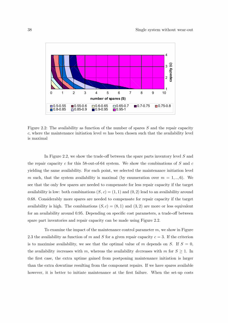
38 Single system without wear-out
0 1 2 3 4 5 6 7 8 9 101
2
3
4
number of spares (S)
capa
city
(c)
0.5-0.55 0.55-0.6 0.6-0.65 0.65-0.7 0.7-0.75 0.75-0.80.8-0.85 0.85-0.9 0.9-0.95 0.95-1
Figure 2.2: The availability as function of the number of spares S and the repair capacityc, where the maintenance initiation level m has been chosen such that the availability levelis maximal
In Figure 2.2, we show the trade-off between the spare parts inventory level S and
the repair capacity c for this 58-out-of-64 system. We show the combinations of S and c
yielding the same availability. For each point, we selected the maintenance initiation level
m such, that the system availability is maximal (by enumeration over m = 1, .., 6). We
see that the only few spares are needed to compensate for less repair capacity if the target
availability is low: both combinations (S, c) = (1, 1) and (0, 2) lead to an availability around
0.68. Considerably more spares are needed to compensate for repair capacity if the target
availability is high. The combinations (S, c) = (8, 1) and (3, 2) are more or less equivalent
for an availability around 0.95. Depending on specific cost parameters, a trade-off between
spare part inventories and repair capacity can be made using Figure 2.2.
To examine the impact of the maintenance control parameterm, we show in Figure
2.3 the availability as function of m and S for a given repair capacity c = 3. If the criterion
is to maximise availability, we see that the optimal value of m depends on S. If S = 0,
the availability increases with m, whereas the availability decreases with m for S ≥ 1. Inthe first case, the extra uptime gained from postponing maintenance initiation is larger
than the extra downtime resulting from the component repairs. If we have spares available
however, it is better to initiate maintenance at the first failure. When the set-up costs
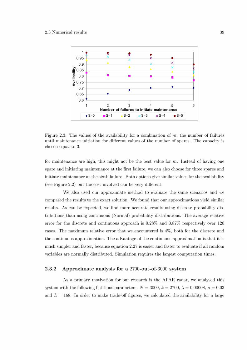
2.3 Numerical results 39
0.60.65
0.70.75
0.80.85
0.9
0.951
1 2 3 4 5 6Number of failures to initiate maintenance
Ava
ilabi
lity
S=0 S=1 S=2 S=3 S=4 S=5
Figure 2.3: The values of the availability for a combination of m, the number of failuresuntil maintenance initiation for different values of the number of spares. The capacity ischosen equal to 3.
for maintenance are high, this might not be the best value for m. Instead of having one
spare and initiating maintenance at the first failure, we can also choose for three spares and
initiate maintenance at the sixth failure. Both options give similar values for the availability
(see Figure 2.2) but the cost involved can be very different.
We also used our approximate method to evaluate the same scenarios and we
compared the results to the exact solution. We found that our approximations yield similar
results. As can be expected, we find more accurate results using discrete probability dis-
tributions than using continuous (Normal) probability distributions. The average relative
error for the discrete and continuous approach is 0.28% and 0.87% respectively over 120
cases. The maximum relative error that we encountered is 4%, both for the discrete and
the continuous approximation. The advantage of the continuous approximation is that it is
much simpler and faster, because equation 2.27 is easier and faster to evaluate if all random
variables are normally distributed. Simulation requires the largest computation times.
2.3.2 Approximate analysis for a 2700-out-of-3000 system
As a primary motivation for our research is the APAR radar, we analysed this
system with the following fictitious parameters: N = 3000, k = 2700, λ = 0.00008, μ = 0.03
and L = 168. In order to make trade-off figures, we calculated the availability for a large
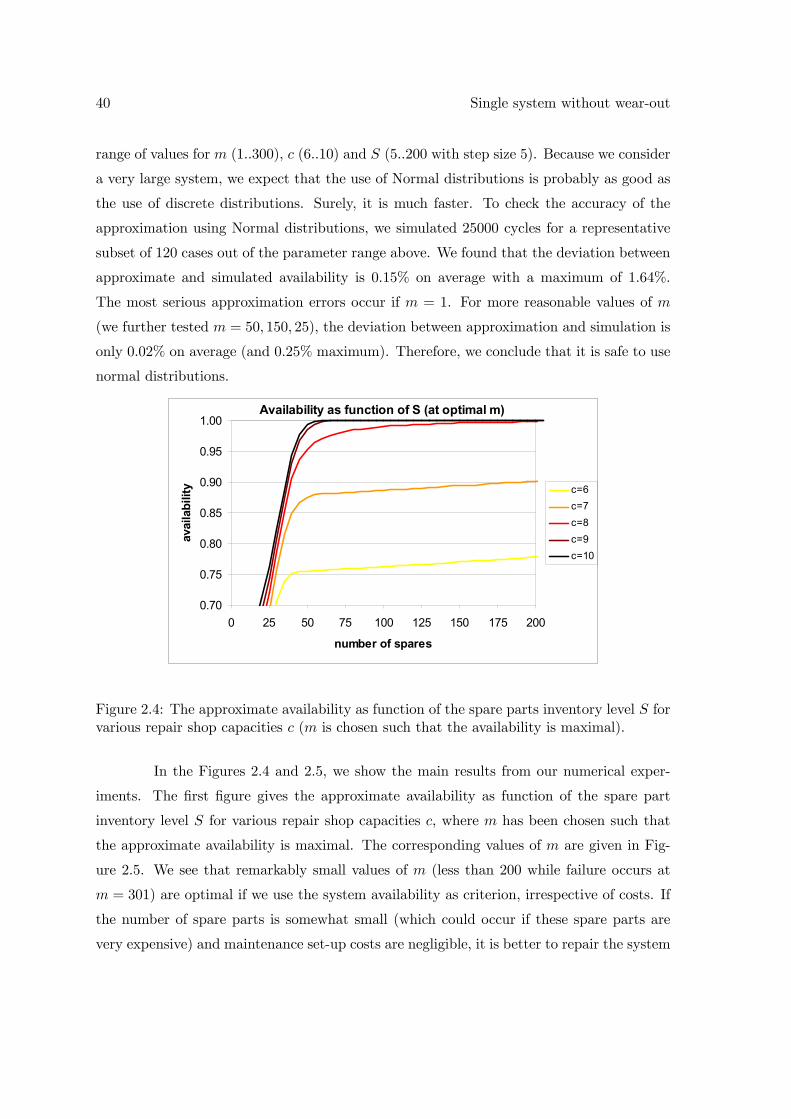
40 Single system without wear-out
range of values for m (1..300), c (6..10) and S (5..200 with step size 5). Because we consider
a very large system, we expect that the use of Normal distributions is probably as good as
the use of discrete distributions. Surely, it is much faster. To check the accuracy of the
approximation using Normal distributions, we simulated 25000 cycles for a representative
subset of 120 cases out of the parameter range above. We found that the deviation between
approximate and simulated availability is 0.15% on average with a maximum of 1.64%.
The most serious approximation errors occur if m = 1. For more reasonable values of m
(we further tested m = 50, 150, 25), the deviation between approximation and simulation is
only 0.02% on average (and 0.25% maximum). Therefore, we conclude that it is safe to use
normal distributions.
Availability as function of S (at optimal m)
0.70
0.75
0.80
0.85
0.90
0.95
1.00
0 25 50 75 100 125 150 175 200
number of spares
avai
labi
lity c=6
c=7c=8c=9c=10
Figure 2.4: The approximate availability as function of the spare parts inventory level S forvarious repair shop capacities c (m is chosen such that the availability is maximal).
In the Figures 2.4 and 2.5, we show the main results from our numerical exper-
iments. The first figure gives the approximate availability as function of the spare part
inventory level S for various repair shop capacities c, where m has been chosen such that
the approximate availability is maximal. The corresponding values of m are given in Fig-
ure 2.5. We see that remarkably small values of m (less than 200 while failure occurs at
m = 301) are optimal if we use the system availability as criterion, irrespective of costs. If
the number of spare parts is somewhat small (which could occur if these spare parts are
very expensive) and maintenance set-up costs are negligible, it is better to repair the system
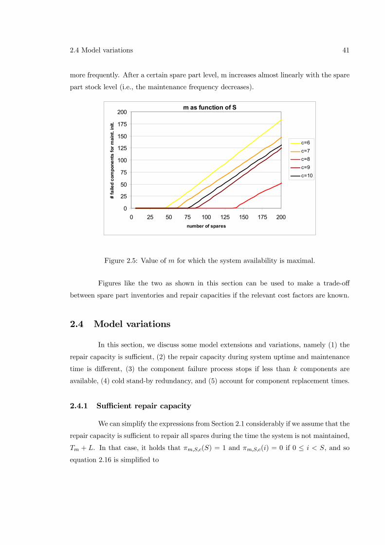
2.4 Model variations 41
more frequently. After a certain spare part level, m increases almost linearly with the spare
part stock level (i.e., the maintenance frequency decreases).
m as function of S
0
25
50
75
100
125
150
175
200
0 25 50 75 100 125 150 175 200number of spares
# fa
iled
com
pone
nts
for m
aint
. ini
t.
c=6c=7c=8c=9c=10
Figure 2.5: Value of m for which the system availability is maximal.
Figures like the two as shown in this section can be used to make a trade-off
between spare part inventories and repair capacities if the relevant cost factors are known.
2.4 Model variations
In this section, we discuss some model extensions and variations, namely (1) the
repair capacity is sufficient, (2) the repair capacity during system uptime and maintenance
time is different, (3) the component failure process stops if less than k components are
available, (4) cold stand-by redundancy, and (5) account for component replacement times.
2.4.1 Sufficient repair capacity
We can simplify the expressions from Section 2.1 considerably if we assume that the
repair capacity is sufficient to repair all spares during the time the system is not maintained,
Tm + L. In that case, it holds that πm,S,c(S) = 1 and πm,S,c(i) = 0 if 0 ≤ i < S, and so
equation 2.16 is simplified to
42 Single system without wear-out
E [Dm,S,c] ≈NX
n=maxS,mE [Rc (n− S, n |n)]Pm(n) (2.31)
Now we can evaluate equation 2.31 simply by substitution of equations 2.5 and
2.17. A drawback of this approximation is that it does not facilitate a proper trade-off
between maintenance policy, spare part inventory and repair capacity. Reducing the repair
capacity may lead to a serious violation of our approximating assumption, so that our
approximation becomes very inaccurate.
2.4.2 Different repair capacities during Tm + L and during maintenance
time
When a system fails and the number of spares is insufficient, it is possible that
additional repair capacity will be deployed. Suppose that the normal repair capacity (during
Tm +L) equals c1 and that the capacity during maintenance equals c2 > c1. We can easily
incorporate this refinement by using repair capacity c = c1 in equation 2.12, affecting the
steady state probabilities πm,S,c(i), and repair capacity c = c2 in equation 2.16, affecting
the mean system maintenance time E [Dm,S,c].
2.4.3 System is shut down after more than N − k component failures
If the system shuts down when less than k components are available, the component
failure process can stop before maintenance starts. The only expression that has to be
modified in that case is the distribution of the number of failed items in the system when
maintenance starts, Pm(n), because we have an upper bound on the number of failed items.
As a consequence, expression equation 2.17 remains valid for m ≤ n ≤ N − k, but theprobability mass for all n ≥ N − k + 1 is concentrated in N − k + 1:
Pm (N − k + 1) =N−mX
i=N−k+1−m
µN −mi
¶e−(N−m−i)λL
³1− e−λL
´i(2.32)
2.4.4 Cold stand-by redundancy
Let us assume that components cannot fail during stand-by status and that the
system is shut down if less than k components are available. Then we have to modify
the expressions regarding the failure process. As the mean time between two successive
2.4 Model variations 43
component failures in the k-out-of-N system equals 1kλ , the time until maintenance initiation
has an Erlang-m distribution with scale parameter kλ, so we modify equations 2.7 and 2.2
respectively to
fm(t) =(kλ)m tm−1
(m− 1)! e−kλt (2.33)
E [Tm] =m
kλ(2.34)
The probability that n components have failed at the start of system maintenance Pm(n)
can easily be derived, as the number of component failures during the lead-time L is Poisson
distributed, with all mass for n ≥ N − k + 1 being concentrated in N − k + 1:
Pm(n) =
⎧⎪⎨⎪⎩(kλL)n−m
(n−m)! e−kλL m ≤ n ≤ N − k
1−N−k−mPi=0
(kλL)i
i! e−kλL n = N − k + 1(2.35)
To derive the mean system uptime during maintenance set-up E [Um], we use that the
probability of this uptime exceeding t equals the probability that at most (N − k − m)components fail until t. As this number of failures is Poisson distributed with mean kλ, we
find
E [Um] =
LZt=0
Pr (Um > t) dt =
LZt=0
N−k−mXi=0
(kλt)i
i!e−kλtdt
Some algebra yields
E [Um] =N − k −m+ 1
kλ− 1
kλe−kλL
N−k−mXi=0
(N − k −m− j) (kλL)i
i!(2.36)
We obtain an analytical expression for the transition probabilities qi,j by substituting the
above expressions in equation 2.18.
2.4.5 Including component replacement times
Next to component repair, component replacement is a part of the maintenance
activities. Let us assume that the time required for a single component replacement v
is deterministic and that the same repair capacity is needed for component repair and
replacement (otherwise the model extension is trivial). Component replacement occurs as
soon as sufficient components have been repaired. Then, the system availability should be
calculated as
Am,S,c =E [Tm] +E [Um]
E [Tm] + L+E [Dm,S,c] +E [Vm](2.37)
44 Single system without wear-out
where Vm denotes the time needed for component replacement. If all repair capacity is used
for component replacement, the fact that the number of failures during the lead-time L is
binominally distributed (see equation 2.17) leads us to:
E [Vm] = v
&m+ (N −m)
¡1− e−λL
¢c
'(2.38)
where dxe denotes the smallest integer larger than or equal to x. However, if only a singlerepair man is used for component replacement while the remaining capacity (c−1) is used forrepair, the steady state probabilities πm,S,c(i) should be modified as well, which influences
E [Dm,S,c]. For the transition probabilities qi,j , we have to take into account that c − 1servers are available to repair components during the replacement time V :
qi,j =NXn=m
Pm(n)
jXh=0
Hm,S,c−1 (min S, S − i+ n , S − h, nv) · (2.39)
∞Zt=0
fm(t)Hm,S,c (S − h, S − j, t+ L) dt
It should be possible to derive a closed form expression for qi,j , but it is clear that this is
complex.
2.5 Conclusions
In this chapter we presented both an exact and approximate method to make a
trade-off between spare part inventories, repair capacity and maintenance policy in a simple
model. The exact method works very well for systems up to 100 components, for larger
systems the approximation can be used. If the number of components is high, as for the
APAR for instance, we recommend to use Normal distributions for convenience and to
reduce computational efforts.
Although we discussed various model extensions, it is clear that this model is just
a first step towards the integration of spare part management and preventive maintenance
optimisation. In the following chapter we extend this model applicable for systems of which
the components show signs of wear-out.
Chapter 3
Single system with wear-out
In this chapter1 we consider a single k-out-of-N system with wear-out of the com-
ponents. Compared to the model in the previous chapter the introduction of wear-out
complicates the analysis considerably. We have different repair jobs, and so we may con-
sider repair priorities to reduce the system downtime. Also, the computation of the system
uptime and particularly the system downtime is more complex. At the same time, the intro-
duction of multiple states allows for a wider class of maintenance policies if the component
states are observable during system uptime.
To introduce component wear-out we extend the component state space. In the
previous chapter we assumed components have only a working state in which it is as-good-
as-new and a failed state. In this chapter we assume that a component can have multiple
states. See for instance Bloch-Mercier (2002) where the wear-out of a component is also
modelled using multiple states. Therefore we have to adjust the model from the previous
chapter and as becomes clear in this chapter extending the number of component states
implies a number of additional complexities. We elaborate the situation in which there
is only one component state added: a degraded state which is in between of the good-as-
new-state and the failed state. This same way of modelling component wear-out is found
in Sarkar and Sarkar (2001). Although, we do not use arbitrary transition distributions.
We assume that a component in a good-as-new state degrades according to an exponential
distribution with parameter λ1 (defined as a transition from state 0 to state 1). From this1This chapter is based on the paper: K.S. de Smidt-Destombes, M.C. van der Heijden and A. van Harten
(2006). On the interaction between maintenance, spare part inventories and repair capacity for a k-out-of-Nsystem with wear-out; European Journal of Operational Research ; 174 (1); 182-200.
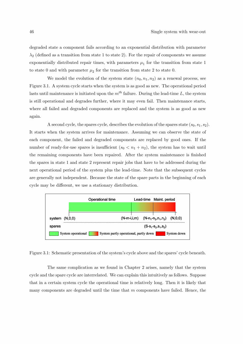
46 Single system with wear-out
degraded state a component fails according to an exponential distribution with parameter
λ2 (defined as a transition from state 1 to state 2). For the repair of components we assume
exponentially distributed repair times, with parameters μ1 for the transition from state 1
to state 0 and with parameter μ2 for the transition from state 2 to state 0.
We model the evolution of the system state (n0, n1, n2) as a renewal process, see
Figure 3.1. A system cycle starts when the system is as good as new. The operational period
lasts until maintenance is initiated upon themth failure. During the lead-time L, the system
is still operational and degrades further, where it may even fail. Then maintenance starts,
where all failed and degraded components are replaced and the system is as good as new
again.
A second cycle, the spares cycle, describes the evolution of the spares state (s0, s1, s2).
It starts when the system arrives for maintenance. Assuming we can observe the state of
each component, the failed and degraded components are replaced by good ones. If the
number of ready-for-use spares is insufficient (s0 < n1 + n2), the system has to wait until
the remaining components have been repaired. After the system maintenance is finished
the spares in state 1 and state 2 represent repair jobs that have to be addressed during the
next operational period of the system plus the lead-time. Note that the subsequent cycles
are generally not independent. Because the state of the spare parts in the beginning of each
cycle may be different, we use a stationary distribution.
Lead-time
(N,0,0) (N-m-i,i,m) (N-n1-n2,n1,n2) (N,0,0)system
spares (S-s1-s2,s1,s2)
Operational time Maint. period
System operational System downSystem partly operational, partly down
Lead-time
(N,0,0) (N-m-i,i,m) (N-n1-n2,n1,n2) (N,0,0)system
spares (S-s1-s2,s1,s2)
Operational time Maint. period
System operational System downSystem partly operational, partly down
Figure 3.1: Schematic presentation of the system’s cycle above and the spares’ cycle beneath.
The same complication as we found in Chapter 2 arises, namely that the system
cycle and the spare cycle are interrelated. We can explain this intuitively as follows. Suppose
that in a certain system cycle the operational time is relatively long. Then it is likely that
many components are degraded until the time that m components have failed. Hence, the
3.1 An analytical approximation 47
number of components in state 1 (n1) is relatively large at the start of maintenance. At
the same time, the number of restored spares (s0) is likely to be relatively large when the
operational time is relatively long. Therefore the system state and the state of the spares
at the beginning of the maintenance period are not independent. As an approximation,
however, we assume both cycles to be independent. Whether this approximation has a
significant impact, is discussed when comparing our approximate methods with results
from discrete event simulation (Section 3.3).
Assuming that all components in state 1 and state 2 are replaced by new ones dur-
ing maintenance and there is no correlation between the system state and the spares state
we compute E [Tm], E [Um] and E [Dm,S,c] exactly in Section 3.1. After discussing compu-
tational issues in Section 3.1.4, we present a model to approximate E [Um] and E [Dm,S,c] in
Section 3.2.The results for both models are given in Section 3.3. Finally, give some model
variation in Section 3.4.
3.1 An analytical approximation
3.1.1 Operational time
The operational time until maintenance initiation Tm is the time until the mth
component failure (1 ≤ m ≤ N − k + 1). If L = 0, it is clear that we should choose
m = N − k + 1. If L > 0, m is likely to be chosen smaller. The distribution function F (t)
for Tm is given by
F (t) = Pr (number of failed components at t ≥ m)
=NXi=m
µN
i
¶(p02(t))
i (1− p02(t))N−i (3.1)
where p02(t), the probability that a component moves from state 0 to state 2
in time t, equals 1 − e−λ1t − λ1λ1−λ2
¡e−λ2t − e−λ1t
¢. Although we could derive E [Tm]
from∞Rt=0
(1 − F (t))dt, it is far easier to use a recursive approach. Let us define Tm(i, j)
as the time needed for a transition from state (N − i− j, i, j) to the set of states inwhich maintenance is initiated (n2 = m). Obviously, we have that Tm(i,m) = 0. If
j < m, the mean value of Tm(i, j) equals the expected sojourn time in the current state
(N − i− j, i, j) plus the expected time needed from the next state on. The expected
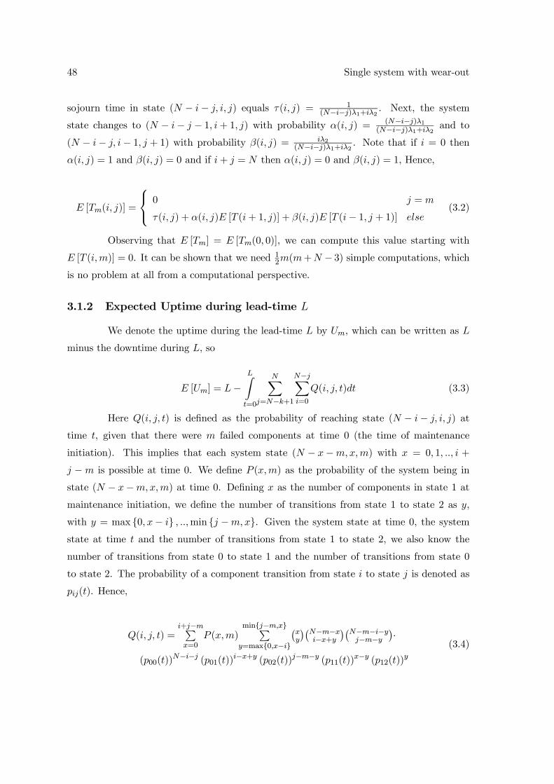
48 Single system with wear-out
sojourn time in state (N − i− j, i, j) equals τ(i, j) = 1(N−i−j)λ1+iλ2 . Next, the system
state changes to (N − i− j − 1, i+ 1, j) with probability α(i, j) = (N−i−j)λ1(N−i−j)λ1+iλ2 and to
(N − i− j, i− 1, j + 1) with probability β(i, j) = iλ2(N−i−j)λ1+iλ2 . Note that if i = 0 then
α(i, j) = 1 and β(i, j) = 0 and if i+ j = N then α(i, j) = 0 and β(i, j) = 1, Hence,
E [Tm(i, j)] =
⎧⎨⎩ 0 j = m
τ(i, j) + α(i, j)E [T (i+ 1, j)] + β(i, j)E [T (i− 1, j + 1)] else(3.2)
Observing that E [Tm] = E [Tm(0, 0)], we can compute this value starting with
E [T (i,m)] = 0. It can be shown that we need 12m(m+N − 3) simple computations, which
is no problem at all from a computational perspective.
3.1.2 Expected Uptime during lead-time L
We denote the uptime during the lead-time L by Um, which can be written as L
minus the downtime during L, so
E [Um] = L−LZt=0
NXj=N−k+1
N−jXi=0
Q(i, j, t)dt (3.3)
Here Q(i, j, t) is defined as the probability of reaching state (N − i− j, i, j) attime t, given that there were m failed components at time 0 (the time of maintenance
initiation). This implies that each system state (N − x−m,x,m) with x = 0, 1, .., i +
j −m is possible at time 0. We define P (x,m) as the probability of the system being in
state (N − x−m,x,m) at time 0. Defining x as the number of components in state 1 atmaintenance initiation, we define the number of transitions from state 1 to state 2 as y,
with y = max 0, x− i , ..,min j −m,x. Given the system state at time 0, the system
state at time t and the number of transitions from state 1 to state 2, we also know the
number of transitions from state 0 to state 1 and the number of transitions from state 0
to state 2. The probability of a component transition from state i to state j is denoted as
pij(t). Hence,
Q(i, j, t) =i+j−mPx=0
P (x,m)minj−m,xPy=max0,x−i
¡xy
¢¡N−m−xi−x+y
¢¡N−m−i−yj−m−y
¢·
(p00(t))N−i−j (p01(t))
i−x+y (p02(t))j−m−y (p11(t))
x−y (p12(t))y
(3.4)
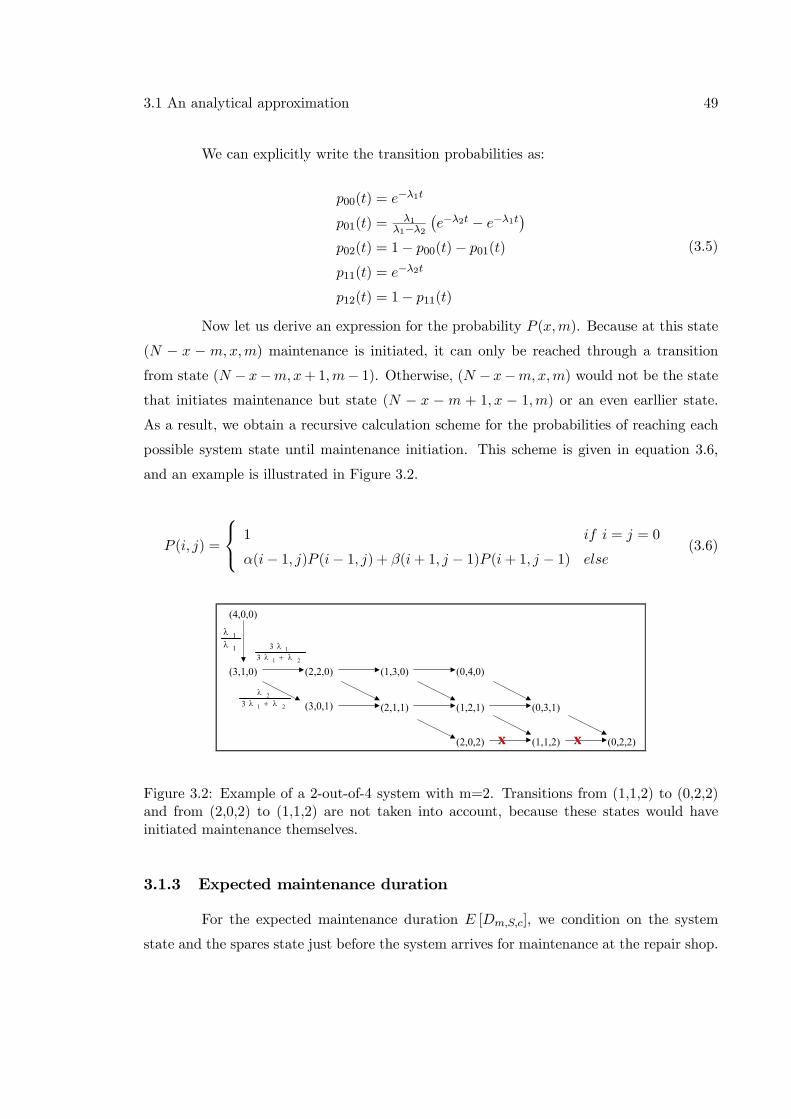
3.1 An analytical approximation 49
We can explicitly write the transition probabilities as:
p00(t) = e−λ1t
p01(t) =λ1
λ1−λ2¡e−λ2t − e−λ1t
¢p02(t) = 1− p00(t)− p01(t)p11(t) = e
−λ2t
p12(t) = 1− p11(t)
(3.5)
Now let us derive an expression for the probability P (x,m). Because at this state
(N − x − m,x,m) maintenance is initiated, it can only be reached through a transitionfrom state (N − x−m,x+1,m− 1). Otherwise, (N − x−m,x,m) would not be the statethat initiates maintenance but state (N − x − m + 1, x − 1,m) or an even earllier state.As a result, we obtain a recursive calculation scheme for the probabilities of reaching each
possible system state until maintenance initiation. This scheme is given in equation 3.6,
and an example is illustrated in Figure 3.2.
P (i, j) =
⎧⎨⎩ 1 if i = j = 0
α(i− 1, j)P (i− 1, j) + β(i+ 1, j − 1)P (i+ 1, j − 1) else(3.6)
(4,0,0)
(3,1,0)
1
1λλ
(2,2,0) (1,3,0) (0,4,0)
(3,0,1) (2,1,1) (1,2,1) (0,3,1)
(2,0,2) (1,1,2) (0,2,2)
21
13
3λ+λ
λ
21
23 λ+λ
λ
XX XX
Figure 3.2: Example of a 2-out-of-4 system with m=2. Transitions from (1,1,2) to (0,2,2)and from (2,0,2) to (1,1,2) are not taken into account, because these states would haveinitiated maintenance themselves.
3.1.3 Expected maintenance duration
For the expected maintenance duration E [Dm,S,c], we condition on the system
state and the spares state just before the system arrives for maintenance at the repair shop.
50 Single system with wear-out
Because we assume that the spares cycle and the system cycle are independent, we have
that:
E [Dm,S,c] =SX
s0=0
S−s0Xs2=0
NXn2=m
N−n2Xn1=0
PL(n1, n2)π(s0, s2) · (3.7)
E [R(n1 + n2 − s0, n1 + S − s0 − s2, n2 + s2)]
PL(n1, n2) is the probability of the system having n1 degraded and n2 failed compo-
nents when actual maintenance activities starts and π(s0, s2) is the steady state probability
of the spares inventory consisting of s0 ready for use spares and s2 failed spares (note that
s1 = S−s0−s2). R(r, es1, es2) is the time to repair r components with capacity c when thereare es1 degraded and es2 failed components available at the start of the repair. Regarding thesystem state at maintenance initiation, we have that n2 = m and PL(n1,m) = P (n1,m) if
L = 0. If L > 0 then PL(n1, n2) = Q(n1, n2, L). We provide expressions for R(r, es1, es2) andπ(s0, s2) respectively.
Repair time R (r, s1, s2) and priority rule
The repair time R (r, s1, s2) depends on the order in which the s1 degraded and
s2 failed components are repaired, which can be given by a certain repair priority rule.
The other way around, the repair priority rule influences the spares state at the start
of system maintenance. For our priority rule we assume the repair time for a degraded
component to be smaller on average than the repair time of a failed component. In other
words, we assume μ1 > μ2. We try to minimise the maintenance duration by repairing as
many degraded components as possible. When the number of degraded components is not
sufficient to replace all failed and degraded components (n1 + s1 < N − s0 − n0), we haveto repair some failed components as well. It is well known that we minimise the makespan
(and hence the system repair time) by selecting the longest mean processing times first, see
Pinedo and Chao (1999). So we use the following repair priority rule:
If there are sufficient degraded spares (in state 1), then only repair degraded components.
If the number of degraded components is insufficient, start repairing the minimum number
of failed components needed to repair the system. Next, repair the degraded components.
If we have both degraded and failed spares to be repaired after system repair, we
need a second repair priority rule. It is logical to aim for handling as many jobs as possible
3.1 An analytical approximation 51
before Tm + L (the time between maintenance instances). Therefore we complete the jobs
with the shortest mean repair time first.
Now let us apply the repair priority rule to find the mean repair time E[R(r, s1, s2)].
We define r = [n1 + n2 − s0]+ as the total number of repairs needed to repair the system.Then we need to restore [r − s1]+ failed spares during the maintenance period. Since wehave at most c spares in the repair shop, we start with the min
©c, [r − s1]+
ªfailed spares
in repair at the start of the repair period. Together with these failed spares we assign
a = min©s1, c−min
©c, [r − s1]+
ªªdegraded spares to the repair shop. If there is still
repair capacity left, we use this capacity for the remainder of the failed components. The
number of failed spares in the repair shop is now equal to b = min s2, c− a. Let us denotethe number of components in state 1 and state 2 in the repair shop at the start of the repair
period by a and b respectively. Using R (r, s1, s2) = 0 if r = 0 or s1 < 0 or s2 < 0, we find
the following recursive relation for the expected repair time:
E [R (r, s1, s2)] =1
aμ1+bμ2+ aμ1
aμ1+bμ2E [R (r − 1, s1 − 1, s2)]
+ bμ2aμ1+bμ2
E [R (r − 1, s1, s2 − 1)](3.8)
Steady state probabilities of the spares states
We use a Markov chain to determine the steady state probabilities π(i). Here
we use a short hand notation i = (s0, s2). We want to solve the steady state conditions
π =MTπ withP
π(i) = 1. Each entry (i, j) of the transition matrixM equals the transition
probability qij that j = (s00, s02) is the spares state just before the maintenance period starts,
while the spares state just before the previous maintenance period was i = (s0, s2). We
calculate the probability qij by conditioning on the time to maintenance initiation T = t:
qij =NP
n2=m
N−n2Pn1=0
PL (n1, n2) ·∞Rt=0
f(t)H¡min
©s1 + n1, [S − s2 − n2]+
ª,min s2 + n2, S , s01, s02, t+ L
¢dt
(3.9)
where f(t) is the density function of T and H (w, x, y, z, t) is the probability that
the spares state changes from w degraded and x failed spares to y degraded and z failed
spares during t with c servers. In the special case L = 0, we have that n2 = m and so the
transition probabilities consist of one summation only. The density function f(t) can be
found as the derivative of F (t) from equation 3.1:
52 Single system with wear-out
f(t) =NXg=m
N−gXh=0
µN
g
¶µN − gh
¶(−1)h(g + h)λ2p01(t) (p02(t))g+h−1 (3.10)
Let us now derive an expression for H (w, x, y, z, t). We first note that only a non-
negative number of spares can be restored, so H (w, x, y, z, t) = 0 if w < y and/or x < z.
Because our repair priority rule states that we should first restore degraded components, it is
not possible to restore one or more failed components if the number of degraded components
remaining is at least equal to the number of servers, thus H (w,x, y, z, t) = 0 if y ≥ c andx > z. If no spares are restored (i.e. w = y and x = z) we have a repair rate that is
equal to min c, wμ1 + min x, c−min c, wμ2 and therefore H (w, x, y, z, t) decreasesexponentially with that rate. If spares are restored, we distinguish two cases: one in which
all spares are being repaired immediately (w+ x ≤ c) and one in which not all repairs, butonly c repairs, start immediately (w + x > c).
In the first case we have a combination of two binomial distributions, one with
parameters w and e−μ1t, and one with parameters x and e−μ2t. In the second case, where
w + x > c, we can write H (w, x, y, z, t) in a recursive formulation. In case w ≤ c, it is
possible to have a failed spare restored before a degraded spares is restored or the other
way around. In case w > c the only possibility is to restore a degraded spare. In the
recursive formulation y and z play the role of fixed parameters, which we suppress for
readability. We find that:
H (w, x, t) =⎧⎪⎪⎪⎪⎪⎪⎪⎪⎪⎪⎪⎪⎪⎪⎪⎪⎪⎨⎪⎪⎪⎪⎪⎪⎪⎪⎪⎪⎪⎪⎪⎪⎪⎪⎪⎩
0w < y ∨ x < z∨ (y ≥ c ∧ x > z)
e−(minc,wμ1+minx,[c−w]+μ2)t w = y ∧ x = z¡
wy
¢¡xz
¢e−(yμ1+zμ2)t
¡1− e−μ1t
¢w−y ¡1− e−μ2t
¢x−zw + x ≤ c
tRτ=0
W (τ) ((c− w)μ2H (w, x− 1, t− τ)
+wμ1H (w − 1, x, t− τ)) dτ
w + x > c ∧ w ≤ c
tRτ=0
wμ1W (τ)H (w − 1, x, t− τ) dτ w + x > c ∧ w > c
(3.11)
Here W (τ) = e−wμ1τe−(c−w)μ2τ . From the equations 3.10 and 3.11 we are able to
determine all the elements qij of the transition matrix M (see equation 3.9).
3.2 An iterative approximation 53
3.1.4 Computational issues
Our approach as described in Sections 3.1.1 till 3.1.3 has several drawbacks. Firstly,
equations 3.3 and equation 3.4 contain binominals of high order and large summations.
Therefore, we encountered numerical problems and long computation times when evaluating
the equations for larger systems (say N > 80). The computation time for a system with
N = 80 components is several hours on a Pentium II, 800 MHz pc. A similar problem
occurs for the maintenance duration (equation 3.7, 3.8 and 3.9). Secondly, we found that
the computation time to evaluate the transition probabilities becomes large even for smaller
problems, because we evaluated the integrals numerically. The number of integrals is very
large because of the recursive character of equation 3.11. The system size for which we
can find the maintenance duration within a reasonable amount of time (less than about an
hour) is up to 10 or 20 components.
3.2 An iterative approximation
Because of the drawbacks of the exact method, we developed simpler and faster
approximations for E [Um] and E [Dm,S,c]. These approximations are based on the first
two moments by fitting an appropriate distribution. For continuous distributions on [0,∞)we use phase type distributions, see Tijms (1994). For discrete distributions on [0, 1, 2, ...)
we use either a mixture of two binomial distributions, a mixture of two negative binomial
distributions, a mixture of two geometric distributions or a Poisson distribution dependent
on the mean and variance, see Adan, Van Eenige and Resing (1995).
3.2.1 Expected uptime during lead-time L
Let us denote the time from maintenance initiation to system failure by bT , thetime from m component failures until the (N − k + 1)th component fails if L → ∞. Thenthe mean uptime during the lead-time equals E
hmin
nbT ,Loi = Eh bTi − E ∙h bT − Li+¸.
We can evaluate such an expression easiliy for specific classes of probability distributions,
particularly for phase type distributions (for example, hyperexponential distributions or
mixtures of Erlang distributions). Therefore, a simple approximation is to calculate the
first two moments of bT exactly and next to approximate the distribution of bT by a mixtureof Erlang distributions with the same first two moments. Such an approach has appeared to
54 Single system with wear-out
be fruitful in many applications where the performance measure to be approximated does
not depend heavily on the tails of the probability distribution, see Tijms (1994).
The first two moments of bT can be found by conditioning on the system state at
maintenance initiation:
Eh bTi = N−mX
i=0
P (i,m)Eh bT (i,m)i (3.12)
Eh bT 2i = N−mX
i=0
P (i,m)Eh bT 2(i,m)i (3.13)
Here bT (i,m) is the time until the (N − k + 1)th component failure occurs whenthe system is in state (N − i−m, i,m) at maintenance initiation. E
h bT (i,m)i is foundanalogously to equation 3.2 with only a small difference in the restriction, which becomes
equal to j = N−k+1. For the second moment, the recursion is not straightforward becausethe transition depends on the sojourn time. After some algebra we find equation 3.14 using
Eh bT 2(i, j)i = 0 if j = N − k + 1.
Eh bT 2(i, j)i = 2τ(i, j)E
h bT (i, j)i+ α(i, j)Eh bT 2(i+ 1, j)i (3.14)
+β(i, j)Eh bT 2(i− 1, j + 1)i (3.15)
3.2.2 Expected maintenance duration
The basic idea for our approximation of the mean system downtime is to use a
moment iteration scheme as has been proposed by De Kok (1989) for the analysis of the
waiting time in the G/G/1 queue. First, we define W1 and W2 as stochastic variables for
the number of repairs of type 1 and type 2 respectively during the maintenance time. We
can approximate the maintenance duration by:
E [D] ≈ E [W1]
cμ1+E [W2]
cμ2(3.16)
This is an approximation, because we pretend that first all c servers are busy with
failed components at a joint rate cμ2 and next they are all busy with degraded components at
a joint rate cμ1. The reality is that failed and degraded items can be repaired simultaneously
and that the repair rate can be less than cμ1 at the end of the maintenance period if less
3.2 An iterative approximation 55
than c components are available, leaving one or more servers idle. The variables W1 and
W2 depend on the system state and the spares state at the start of maintenance. We define
Ai as the number of system components and Bi as the number of spare components in state
i (i = 0, 1, 2) when the system arrives for maintenance. Because of our repair priority rule,
failed spares are only repaired if the total number of failed components exceeds the number
of spares S, hence:
W2 = [A2 +B2 − S]+ (3.17)
The number of type 1 repairs equals the total number of components needed,
which equals [N −A0 −B0]+, minus the components that are obtained by repairing failedcomponents:
W1 = [N −A0 −B0]+ −W2 (3.18)
The variables Bi depend on the number of spares in each state at the end of the
previous maintenance period. Defining the variables Ci as the number of spare components
in state i after the maintenance is finished:
C0 = [B0 − (A1 +A2)]+ = [B0 +A0 −N ]+ (3.19)
C1 = S − C0 − C2 (3.20)
C2 = min A2 +B2, S (3.21)
Because we start with repairing the type 1 spares when maintenance is finished,
C1 decreases with the number of type 1 spares that can be repaired during T + L with
capacity c and repair rate μ1, which is denoted by Zμ1(T +L). If there is any time left, C2
decreases with the number of failed spares that can be restored during the remaining time.
Therefore we denote Rμ1(C1) as the time needed to restore C1 components with repair rate
μ1 and capacity c. For Bi we find:
B0 = S −B1 −B2 (3.22)
B1 =£C1 − Zμ1 (T + L)
¤+ (3.23)
B2 =hC2 − Zμ2
³£T + L−Rμ1(C1)
¤+´i+ (3.24)
56 Single system with wear-out
Unfortunately, we face correlations between Ai and Bi. To simplify calculations
we assume that B1 = 0. This means that T + L is long enough to restore all spares that
are degraded at the end of the maintenance period. This is a reasonable assumption, since
the degraded spares have priority to be repaired. The set of equations is simplified to:
B0 = S −B2 (3.25)
B2 =£C2 − Zμ2
¡T + L−Rμ1(C1)
¢¤+ (3.26)
C0 = [B0 +A0 −N ]+ (3.27)
C1 = S − C0 − C2 (3.28)
C2 = min A2 +B2, S (3.29)
Now we find E [W1] and E [W2] using the following moment iteration algorithm:
Step 0: set the first two moments of B2 to 0, determine the first two moments of
A0 and A2
Step 1: fit a discrete distribution to A2 +B2 assuming that A2 and B2 are uncor-
related.
Step 2: determine the first two moments of B0, using equation 3.25 and fit a
discrete distribution for A0 +B0 assuming that A0 and B0 are uncorrelated.
Step 3: calculate the mean and variance of C0 and C2 using two moment approx-
imations (equations 3.27 and 3.29).
Step 4: calculate the mean and variance of C1 from equation 3.28 taking into
account cov(C1, C2).
Step 5: calculate the mean and variance of B2 by approximating the first two
moments of X = S − (C2 − Zμ2
¡T + L−Rμ1(C1)
¢) and using B2 = [S −X]+.
Step 6: determine E [W2] and E [W1] from equations 3.17 and 3.18 using the mean
of W = [N − (A0 +B0)]+. If the convergence criterion is not satisfied then go to step 1,otherwise stop.
The first two moments of A0 and A2 that we need for step 0 are relatively easy to
find:
3.2 An iterative approximation 57
E [A0] =N−mXi=0
P (i,m)(N −m− i)p00(L) (3.30)
E£A20¤=N−mXi=0
P (i,m)(N −m− i)p00(L) 1− p00(L) + (N −m− i)p00(L) (3.31)
E [A2] = m+N−mXi=0
P (i,m) (N −m− i)p02(L) + ip12(L) (3.32)
E£A22¤=N−mXi=0
P (i,m) (N −m− i)p02(L) 1− p02(L) + (N −m− i)p02(L) (3.33)
+ ip12(L) 1− p12(L) + ip12(L)+ 2i(N −m− i)p02(L)p12(L)
+ 2m(N − i−m)p02(L) + 2mip12(L) +m2ª
For step 2 we have E [B0] = S − E [B2] and var [B0] = var [B2] and we are ableto fit a distribution for A0 +B0.
For step 3 we have a distribution for A0 + B0 from step 1, which allows us to
determine E [C0] and var [C0]. E [C2] and var [C2] are found using the distribution we
found for A2 +B2 in step 0 or in step 5.
In step 4 we use equations 3.34 and 3.35 with only the covariance as unknown
term.
E [C1] = S −E [C0]−E [C2] (3.34)
var [C1] = var [C0]− var [C2]− 2cov [C1, C2] (3.35)
For cov [C1, C2] we condition on A1:
cov [C1, C2] = E [cov [C1, C2 |A1 ]] + cov [E [C1 |A1 ] , E [C2 |A1 ]] (3.36)
= cov [min A1, S − C2 , C2] = Pr (A1 > S − C2) cov [S − C2, C2]
= −var [C2] Pr (A1 > S − C2) = −var [C2] Pr (N −A0 +B2 > S)
= −var [C2] Pr (A0 +B0 < N)
58 Single system with wear-out
In step 5 we define X = S −¡C2 − Zμ2
¡T + L−Rμ1(C1)
¢¢and we approximate
the mean and variance of Rμ1 (C1) and Zμ2 (X) by:
E£Rμ1 (C1)
¤≈ E [C1]
cμ1(3.37)
var£Rμ1 (C1)
¤≈ E [C1](cμ1)
2 +var [C1]
(cμ1)2 (3.38)
E£Zμ2 (X)
¤≈ cμ2E [X] (3.39)
var£Zμ2(X)
¤≈ cμ2E [X] + (cμ2)2 var [X] (3.40)
The mean and variance of X are now written by:
E [X] = S −E [C2] + cμ2µE [T ] + L− E [C1]
cμ1
¶(3.41)
var [X] = cμ2
µE [T ] + L− E [C1]
cμ1
¶+ (cμ2)
2 var [T ] +
µμ2μ1
¶2(E [C1] + var [C1]) (3.42)
+ var [C2] + 2μ2μ1cov [C1, C2]
For B2 we find E [B2] = E£[S −X]+
¤and var [B2] = var
£[S −X]+
¤. With the
mean and variance for A2 from step 0 and the mean and variance for B2 from step 4, we
fit a discrete distribution to A2 +B2.
In step 6 we determine E [W2] using the distribution we found for A2 + B2 in
step 5. We use the distribution for A0 + B0 to find the mean for the total workload
W = [N −A0 −B0]+. Then E [W1] is found by E [W ]−E [W2].
3.3 Numerical results
Because both methods as discussed in Sections 3.1 and 3.2 are approximations, we
need to test the accuracy of both methods. To this end, we constructed a discrete event
simulation model as benchmark. The simulation results given in this paper are based on
5000 cycles.
We computed over 460 scenarios divided into three different system sizes: 7-out-
of-10 system, 58-out-of-64 system and 2700-out-of-3000 system.
In Table 3.1 we give an overview of the different scenarios we used. We used the
method presented in Section 3.1 (if feasible within a few hours computation time), denoted
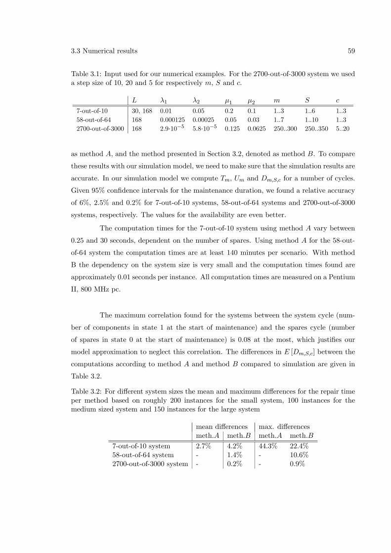
3.3 Numerical results 59
Table 3.1: Input used for our numerical examples. For the 2700-out-of-3000 system we useda step size of 10, 20 and 5 for respectively m, S and c.
L λ1 λ2 μ1 μ2 m S c
7-out-of-10 30, 168 0.01 0.05 0.2 0.1 1..3 1..6 1..358-out-of-64 168 0.000125 0.00025 0.05 0.03 1..7 1..10 1..32700-out-of-3000 168 2.9·10−5 5.8·10−5 0.125 0.0625 250..300 250..350 5..20
as method A, and the method presented in Section 3.2, denoted as method B. To compare
these results with our simulation model, we need to make sure that the simulation results are
accurate. In our simulation model we compute Tm, Um and Dm,S,c for a number of cycles.
Given 95% confidence intervals for the maintenance duration, we found a relative accuracy
of 6%, 2.5% and 0.2% for 7-out-of-10 systems, 58-out-of-64 systems and 2700-out-of-3000
systems, respectively. The values for the availability are even better.
The computation times for the 7-out-of-10 system using method A vary between
0.25 and 30 seconds, dependent on the number of spares. Using method A for the 58-out-
of-64 system the computation times are at least 140 minutes per scenario. With method
B the dependency on the system size is very small and the computation times found are
approximately 0.01 seconds per instance. All computation times are measured on a Pentium
II, 800 MHz pc.
The maximum correlation found for the systems between the system cycle (num-
ber of components in state 1 at the start of maintenance) and the spares cycle (number
of spares in state 0 at the start of maintenance) is 0.08 at the most, which justifies our
model approximation to neglect this correlation. The differences in E [Dm,S,c] between the
computations according to method A and method B compared to simulation are given in
Table 3.2.
Table 3.2: For different system sizes the mean and maximum differences for the repair timeper method based on roughly 200 instances for the small system, 100 instances for themedium sized system and 150 instances for the large system
mean differences max. differencesmeth.A meth.B meth.A meth.B
7-out-of-10 system 2.7% 4.2% 44.3% 22.4%58-out-of-64 system - 1.4% - 10.6%2700-out-of-3000 system - 0.2% - 0.9%
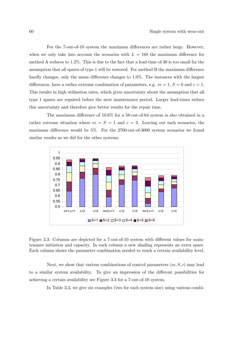
60 Single system with wear-out
For the 7-out-of-10 system the maximum differences are rather large. However,
when we only take into account the scenarios with L = 168 the maximum difference for
method A reduces to 1.2%. This is due to the fact that a lead-time of 30 is too small for the
assumption that all spares of type 1 will be restored. For method B the maximum difference
hardly changes, only the mean difference changes to 1.0%. The instances with the largest
differences, have a rather extreme combination of parameters, e.g. m = 1, S = 6 and c = 1.
This results in high utilisation rates, which gives uncertainty about the assumption that all
type 1 spares are repaired before the next maintenance period. Larger lead-times reduce
this uncertainty and therefore give better results for the repair time.
The maximum difference of 10.6% for a 58-out-of-64 system is also obtained in a
rather extreme situation where m = S = 1 and c = 3. Leaving out such scenarios, the
maximum difference would be 5%. For the 2700-out-of-3000 system scenarios we found
similar results as we did for the other systems.
0.50.550.6
0.650.7
0.750.8
0.850.9
0.951
m=1,c=1 c=2 c=3 m=2,c=1 c=2 c=3 m=3,c=1 c=2 c=3
S=1 S=2 S=3 S=4 S=5 S=6
Figure 3.3: Columns are depicted for a 7-out-of-10 system with different values for main-tenance initiation and capacity. In each column a new shading represents an extra spare.Each column shows the parameter combination needed to reach a certain availability level.
Next, we show that various combinations of control parameters (m,S, c) may lead
to a similar system availability. To give an impression of the different possibilities for
achieving a certain availability see Figure 3.3 for a 7-out-of-10 system.
In Table 3.3, we give six examples (two for each system size) using various combi-
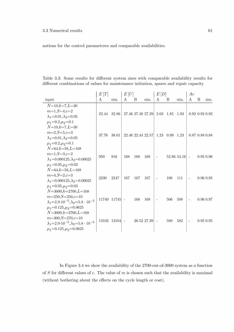
3.3 Numerical results 61
nations for the control parameteres and comparable availabilities.
Table 3.3: Some results for different system sizes with comparable availability results fordifferent combinations of values for maintenance initiation, spares and repair capacity
E [T ] E [U ] E [D] Avinput A sim. A B sim. A B sim. A B sim.
N=10,k=7,L=30m=1,S=4,c=2λ1=0.01,λ2=0.05μ1=0.2,μ2=0.1
22.44 22.86 27.46 27.48 27.29 2.03 1.85 1.93 0.92 0.92 0.92
N=10,k=7,L=30m=2,S=5,c=3λ1=0.01,λ2=0.05μ1=0.2,μ2=0.1
37.76 38.01 22.46 22.44 22.57 1.23 0.99 1.23 0.87 0.88 0.88
N=64,k=58,L=168m=1,S=3,c=2λ1=0.000125,λ2=0.00025μ1=0.05,μ2=0.03
950 916 168 168 168 - 52.86 54.16 - 0.95 0.96
N=64,k=58,L=168m=4,S=2,c=3λ1=0.000125,λ2=0.00025μ1=0.05,μ2=0.03
2230 2247 167 167 167 - 108 111 - 0.96 0.95
N=3000,k=2700,L=168m=250,S=250,c=10λ1=2.9·10−5,λ2=5.8 · 10−5μ1=0.125,μ2=0.0625
11740 11745 - 168 168 - 506 508 - 0.96 0.97
N=3000,k=2700,L=168m=300,S=270,c=10λ1=2.9·10−5,λ2=5.8 · 10−5μ1=0.125,μ2=0.0625
13102 13104 - 26.52 27.39 - 580 582 - 0.95 0.95
In Figure 3.4 we show the availability of the 2700-out-of-3000 system as a function
of S for different values of c. The value of m is chosen such that the availability is maximal
(without bothering about the effects on the cycle length or cost).
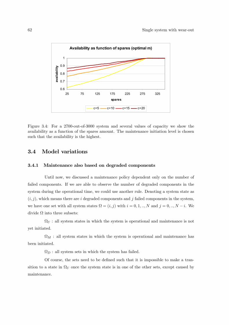
62 Single system with wear-out
Availability as function of spares (optimal m)
0.6
0.7
0.8
0.9
1
25 75 125 175 225 275 325
spares
avai
labi
lity
c=5 c=10 c=15 c=20
Figure 3.4: For a 2700-out-of-3000 system and several values of capacity we show theavailability as a function of the spares amount. The maintenance initiation level is chosensuch that the availability is the highest.
3.4 Model variations
3.4.1 Maintenance also based on degraded components
Until now, we discussed a maintenance policy dependent only on the number of
failed components. If we are able to observe the number of degraded components in the
system during the operational time, we could use another rule. Denoting a system state as
(i, j), which means there are i degraded components and j failed components in the system,
we have one set with all system states Ω = (i, j) with i = 0, 1, .., N and j = 0, .., N − i. Wedivide Ω into three subsets:
ΩU : all system states in which the system is operational and maintenance is not
yet initiated.
ΩM : all system states in which the system is operational and maintenance has
been initiated.
ΩD : all system sets in which the system has failed.
Of course, the sets need to be defined such that it is impossible to make a tran-
sition to a state in ΩU once the system state is in one of the other sets, except caused by
maintenance.
3.4 Model variations 63
The expression for the operational time until maintenance initiation only changes
slightly. In equation 3.2, the condition j = m changes into (i, j) ∈ ΩM . For the expecteduptime during the lead-time, equation 3.3 remains unchanged because the definition of a
failed system remains unchanged. We define a subset of ΩM with only the system states
that initiate maintenance, thus the system states (i, j) ∈ ΩM with (i + 1, j − 1) /∈ ΩM or
(i − 1, j) /∈ ΩM , denoted by ΩI . The uptime is estimated using the equations of Section3.2.1. Taking into account the number of degraded components, the expressions for E
h bTiand var
h bTi are modified by replacing m by j and we sum over (i, j) ∈ ΩI . In expression3.6, for P (i, j) we only change the restriction j = m into (i, j) ∈ ΩI . For the expectedmaintenance duration, we only change E [Ai] and E
£A2i¤for i = 0, 1, 2. This change is
similar to the other changes: replace m by j and sum over (i, j)²ΩI .
Note that a maintenance policy should define the set ΩM . Optimisation of such a
maintenance policy is not straightforward, but at least we are able to evaluate the conse-
quences of a given choice. Explicit optimisation is subject for further research.
3.4.2 Replacement of failed components only
If it is impossible to distinguish the condition of type 0 and 1 components, we
can only replace failed components during maintenance. The system state at the start of
a cycle is then unknown and could be any state (N − i, i, 0) with 0 ≤ i ≤ N −m. As aconsequence we cannot use E [Tm(0, 0)] because the system is not as-good-as-new at the
start of the cycle. We adjust the equation to:
E [Tm] =N−mXi=0
Pstart(i)E [T (i, 0)] (3.43)
Here Pstart(i) is the probability that the system state at the start of a cycle is
equal to (N− i, i, 0). This probability Pstart(i) equals the sum of probabilities of the systembeing in state (N − i− j, i, j) with j = m, ..,N−i at the start of the preceding maintenanceperiod.
Pstart(i) =N−iXj=m
Pmaint(i, j) (3.44)
64 Single system with wear-out
Here Pmaint(i, j) is the probability that the system state equals (N − i− j, i, j)at the start of maintenance. This probability depends on the system state at maintenance
initiation and state transitions during the lead-time:
Pmaint(i, j) =
i+j−mXh=0
Pinit(h,m)Ptrans ((h,m), (i, j), L) j ≥ m (3.45)
Here Ptrans ((h,m), (i, j), L), the probability of a transition from state (N − h −m,h,m) to state (N − i− j, i, j) in time L, which is given by:
Ptrans ((h,m), (i, j), L) =
minj−m,hXy=[h−i]+
µh
y
¶µN − h−mN − i− j
¶µi+ j − h−mj − y −m
¶(p00(L))
N−i−j
× (p01(L))i+y−h (p02(L))j−y−m (p11(L))h−y (p12(L))y
The probability Pinit(h,m) is defined as the probability of the system state being
(N − h−m,h,m) at maintenance initiation, which is a function of the system state at the
start of the cycle:
Pinit(i,m) =i+mXh=0
Pstart(h)Ph,m(i,m) (3.46)
Ph,m(i, j) is the probability of reaching state (N − i− j, i, j) given initial state(N − h, h, 0) and maintenance initiation at m failed components. This probability is found
recursively using:
Ph,m(i, j) =
⎧⎨⎩ 1 (i, j) = (h, 0)
α(i− 1, j)Ph,m(i− 1, j) + β(i+ 1, j − 1)Ph,m(i+ 1, j − 1) else
By filling in equation 3.46 into equation 3.45 filled into equation 3.44 we have a set
of equations with only Pstart(i) which can be solved usingN−mPi=0
Pstart(i) = 1. With Pstart(i),
we have E [Tm].
For the uptime during the lead-time we can use our approximation with Pinit(i,m) =
P (i,m).
For the maintenance duration our model becomes less complex because we only
have type 2 components in our repair shop. This enables us to use the method we used
3.4 Model variations 65
in our model without ageing (see De Smidt-Destombes, Van Der Heijden and Van Harten
(2004)) with the repair rate equal to μ2.
For large systems we encounter the same problem with Ptrans((h,m), (i, j), L) as
we did before with Q(i, j, t). An alternative is to use a moment iteration approach. To find
the distribution of the system being in state (N − i, i, 0) is equal to finding the distributionof A1 with the first two moments:
E [A1] =N−mXi=0
P (i,m) (N −m− i)p01(L) + ip11(L) (3.47)
E£A21¤=N−mXi=0
P (i,m) (N −m− i)p01(L) 1− p01(L) + (N −m− i)p01(L) (3.48)
+ ip11(L) 1− p11(L) + ip11(L)+ 2i(N −m− i)p01(L)p11(L)
The distribution of P (i,m) is the only expression that changes. We start by
choosing an initial distribution for A1. Then we determine P (i,m) using the recursion of
equation 3.2. We then have E [A1] and E£A21¤. By iteration we find the system state
distribution at the start of the cycle.
3.4.3 Stochastic lead-time L
In our model we assumed the lead-time to be deterministic. In case of a stochastic
lead-time we have to adjust the calculations for E [Um] and E [Dm,S,c]. For method A this
means changing equations 3.3 and 3.4. We could do this by conditioning on the lead-time.
Equation 3.4 results in terms of the form exL. The expectation of these terms is found using
the Laplace transform of L and taking a Gamma function for instance. Adjusting equation
3.3 can also be done but takes more effort.
In method B only the second expectation of E [Um] = Eh bTi − E ∙h bT − Li+¸
changes. Because bT and L are independent it is rather easy. For E [Dm,S,c] the equation3.26 for B2 and the equations for the first and second moment of A0 and A2 change. In
equation 3.26 we need Zμ2(Tm+L−Rμ1(C1)) for which the mean and variance are still the
same because Tm, L and Rμ1(C1) are independent of one another. The expressions for the
moments of Ai we condition on L and find terms of the form exL. The expectation of these
terms is found by using Laplace transforms and a Gamma distribution for L for instance.
66 Single system with wear-out
See for a more detailed explanation Chapter 4 or De Smidt-Destombes, Van der Heijden
and Van Harten (2006a).
3.4.4 Cold stand-by redundancy
If components are easily switched on, it may be possible to have the components
that are not necessary for the system turned off. This results in a system with k active
components that degrade while being used, whereas the other components are inactive and
therefore are not subject to degradation. This variant is known as cold stand-by redundancy.
This changes the transition probabilities between and the sojourn times in system states. For
E [Tm] we modify E [Tm(i, j)] from equation 3.2. We change τ(i, j) = 1(k−i)λ1+iλ2 , α(i, j) =
(k−i)λ1(k−i)λ1+iλ2 and β(i, j) = iλ2
(k−i)λ1+iλ2 . For E [Um] we are able to use the approximation
given in method B, for which Eh bT (i, j)i, E h bT 2(i, j)i and P (i, j) changes equivalently to
E [Tm]. For E [Dm,S,c] the only parameters effected in method B are the Ai. If we assume
L = 0 then we know the first and second moment for Ai by using P (i,m). When L > 0,
we encounter difficulties with the determination of the first and second moment. This is
caused by the fact that we need to take into account the exact timing of the transitions.
Otherwise we do not know the number of components in state 0 that are subject to failure.
Hence, we can analyse cold stand-by redundancy if L = 0, but need another
approach if L > 0.
3.5 Conclusions
In this chapter, we introduced component wear-out in a model for the trade-off
between spare part inventories, repair capacity and maintenance policy. This extension
implies a lot of complications. The first complication is the correlations between different
parameters. The state of the spares at the start of maintenance is not independent of the
state of the system at the start of maintenance. Even if we ignore this correlation, we found
it impossible to compute the different expressions we need to determine the availability. On
the one hand it is impossible because of large binomials in the expression for the uptime
during the lead-time. On the other hand it is impossible because of the large state space for
the spares needed to compute the steady state probabilities of the spares at the start of the
maintenance period. Especially if we want to use the model presented in the paper as a basic
model for an optimisation between cost and availability we are in need of an accurate model
3.5 Conclusions 67
with small computation times. Our numerical examples show that the second approximation
(Section 3.2) fulfils these requirements and can be used for this purpose.

68 Single system with wear-out
Chapter 4
Multiple systems without wear-out
The previous two chapters are concerned with the availability of a single k-out-of-
N system. In this chapter1 we consider multiple k-out-of-N systems that share the same
resources. They share the available spare parts and the repair capacity. It is harder to use
the same condition-based maintenance rule as we did for a single system when the spares
and capacity are used for several systems because we could end up with a queue in front of
the repair shop, if two or more systems reach the critical condition (almost) simultaneously.
Obviously it is not very attractive to have systems lined up while they are not even failed
yet. So therefore when we are dealing with more than one system we choose a time-based
maintenance rule. At the same time this helps to spread the work load in the repair shop
more equally.
We consider an installed base of M > 1 identical k-out-of-N systems with hot
stand-by redundancy. We assume that each system is maintained with a fixed maintenance
interval of length T . In other words, we use a block replacement policy with no action
taken if the system fails before its maintenance period. We assume that when a system has
failed and less than k components are working, the system is not shut down. As an example,
consider the APAR that can still work if less than 2700 out of the 3000 transmit-and-receive
elements are available, although the performance is inferior (but better than nothing).
Therefore, the components are still subject to failure after system failure. Just like for the
single system without component wear-out, we assume the components to fail independently
1This chapter is based on the paper: K.S. de Smidt-Destombes, M.C. van der Heijden and A. van Harten;Spare parts analysis for k-out-of-N systems under block replacement and finite repair capacity; InternationalJournal of Production Economics ; to appear.
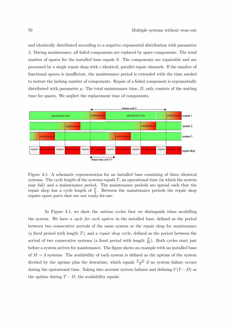
70 Multiple systems without wear-out
and identically distributed according to a negative exponential distribution with parameter
λ. During maintenance, all failed components are replaced by spare components. The total
number of spares for the installed base equals S. The components are repairable and are
processed by a single repair shop with c identical, parallel repair channels. If the number of
functional spares is insufficient, the maintenance period is extended with the time needed
to restore the lacking number of components. Repair of a failed component is exponentially
distributed with parameter μ. The total maintenance time, D, only consists of the waiting
time for spares. We neglect the replacement time of components.
system 1
system 2
system 3
repair shop
maintenance
maintenance
maintenance
maintenancemaintenancemaintenance
operational time
repairs repairsrepairs
maintenance
maintenance
maintenance
maintenancemaintenancemaintenance
operational time
repairs repairsrepairs
System cycle T
Repair shop cycle T/3
system 1
system 2
system 3
repair shop
maintenance
maintenance
maintenance
maintenancemaintenancemaintenance
operational time
repairs repairsrepairs
maintenance
maintenance
maintenance
maintenancemaintenancemaintenance
operational time
repairs repairsrepairs
System cycle T
Repair shop cycle T/3
Figure 4.1: A schematic representation for an installed base consisting of three identicalsystems. The cycle length of the systems equals T , an operational time (in which the systemmay fail) and a maintenance period. The maintenance periods are spread such that therepair shop has a cycle length of T3 . Between the maintenance periods the repair shoprepairs spare parts that are not ready-for-use.
In Figure 4.1, we show the various cycles that we distinguish when modelling
the system. We have a cycle for each system in the installed base, defined as the period
between two consecutive arrivals of the same system at the repair shop for maintenance
(a fixed period with length T ), and a repair shop cycle, defined as the period between the
arrival of two consecutive systems (a fixed period with length TM ). Both cycles start just
before a system arrives for maintenance. The figure shows an example with an installed base
of M = 3 systems. The availability of each system is defined as the uptime of the system
divided by the uptime plus the downtime, which equals T−DT if no system failure occurs
during the operational time. Taking into account system failures and defining U(T −D) asthe uptime during T −D, the availability equals:
71
Av =E [U(T −D)]
T(4.1)
The maintenance duration D depends on the number of failed system components
and the number of spares available at the start of maintenance as well as the repair capac-
ity. Assuming that the failure rate and repair rate are known, we can control the system
availability by the cycle length T , the number of spares S and repair capacity c. Hence, we
should denote the maintenance duration as DT,S,c but for simplicity we omit the subscripts.
For the analysis of this system, queueing models seem to be suitable at first sight.
The repair shop can be modelled as a multi-server queue with batch arrivals, similar to the
DX/M/c queue. The time between the arrivals of batches is deterministic (equal to TM ) and
the number of components in each batch is a random variable that, unfortunately, depends
on the system uptime T − D and is therefore dependent on the repair shop performance.
If the repair shop is highly utilised, the maintenance duration D increases, so the system
uptime T −D decreases and so the work offered to the repair shop decreases. Theoretically,
it is even possible that D > T , and then there are no failed components offered to the
repair shop in the next cycle. As a consequence, the system is always stable having a
utilisation of at most 1. Of course, the system availability is very low if the repair shop
capacity is low. We also observe that it is not straightforward to estimate the repair shop
utilisation in advance because of the relation between repair shop capacity and component
arrival rate. Therefore, we have to use approximations or simulations to estimate the repair
shop utilisation. We conclude that the repair shop can be modelled as a non standard
queueing system for which no suitable results are available in the literature to the best of
our knowledge.
As another option, it seems to be logical to use renewal theory. However, we face
the complication that consecutive system cycles are (possibly heavily) correlated, which
induces correlations between repair shop cycles as well. We can explain this as follows using
Figure 4.2.
A k-out-of-N system arrives every T time units for maintenance. Maintenance
is finished as soon as sufficient ready-for-use components are available to replace all failed
components, which takes some time D (where D = 0 if the number of functional spares
is sufficient to replace all failed components immediately). The operational time in the
next system cycle equals the time until the start of the next system maintenance, T −D.
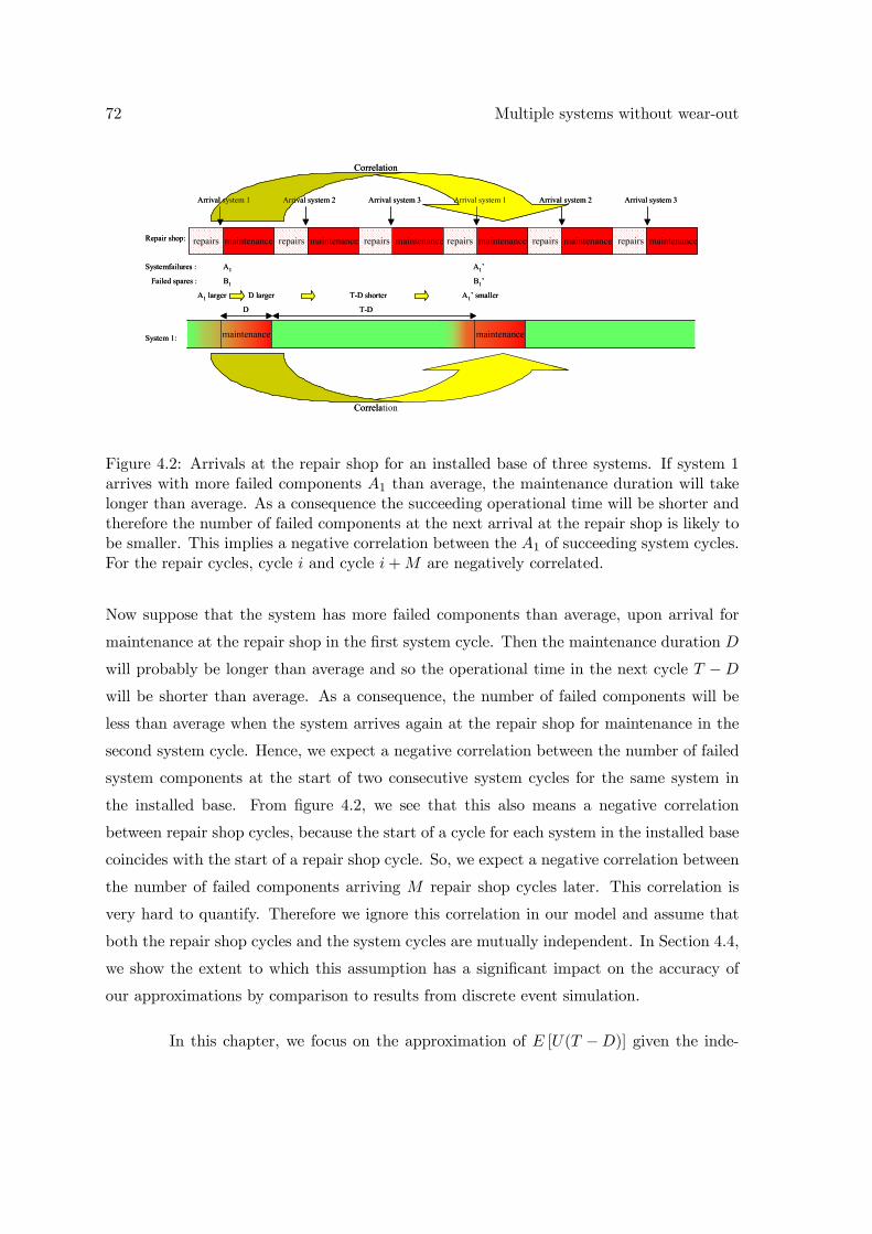
72 Multiple systems without wear-out
maintenancemaintenancemaintenance repairs repairsrepairs maintenancemaintenance repairs repairsrepairs maintenance
Arrival system 1 Arrival system 2 Arrival system 3 Arrival system 1 Arrival system 2 Arrival system 3
Repair shop:
Systemfailures :
Failed spares :
System 1:
A1
B1
A1’
B1’
maintenance maintenance
A1 larger D larger T-D shorter A1’ smaller
D T-D
Correlation
Correlation
Figure 4.2: Arrivals at the repair shop for an installed base of three systems. If system 1arrives with more failed components A1 than average, the maintenance duration will takelonger than average. As a consequence the succeeding operational time will be shorter andtherefore the number of failed components at the next arrival at the repair shop is likely tobe smaller. This implies a negative correlation between the A1 of succeeding system cycles.For the repair cycles, cycle i and cycle i+M are negatively correlated.
Now suppose that the system has more failed components than average, upon arrival for
maintenance at the repair shop in the first system cycle. Then the maintenance duration D
will probably be longer than average and so the operational time in the next cycle T −Dwill be shorter than average. As a consequence, the number of failed components will be
less than average when the system arrives again at the repair shop for maintenance in the
second system cycle. Hence, we expect a negative correlation between the number of failed
system components at the start of two consecutive system cycles for the same system in
the installed base. From figure 4.2, we see that this also means a negative correlation
between repair shop cycles, because the start of a cycle for each system in the installed base
coincides with the start of a repair shop cycle. So, we expect a negative correlation between
the number of failed components arriving M repair shop cycles later. This correlation is
very hard to quantify. Therefore we ignore this correlation in our model and assume that
both the repair shop cycles and the system cycles are mutually independent. In Section 4.4,
we show the extent to which this assumption has a significant impact on the accuracy of
our approximations by comparison to results from discrete event simulation.
In this chapter, we focus on the approximation of E [U(T −D)] given the inde-
4.1 Model analysis 73
pendence assumption as stated above. We derive a set of stochastic equations for the
maintenance duration D. We present two approximation methods to solve the system of
equations for D based on the first two moments of the key random variables involved. The
first approximation is based on continuous probability distributions (particularly suitable for
large systems) and the second approximation is based on discrete probability distributions
(particularly suitable for small systems).
4.1 Model analysis
As stated before, we need to determine the expected uptime U(T − D) of thesystem during the operational time T −D. In the remainder of this thesis, we simply usethe shorthand notation U . If the system is still operational when it arrives for maintenance
(i.e. the number of failed components is at most N−k), we have that U = T −D. However,if the system fails before maintenance starts, the uptime equals the time until system failure.
Let us use eU to denote the system time to failure if there is no maintenance. Then we can
write U = minT −D, eU. It is easy to find eU as we show at the end of Section 4.2. The
unknown variable we focus on first is the maintenance duration D. Before we do so, we give
a list of the assumptions we use throughout this chapter.
1. All components have the same exponentially distributed time to failure.
2. The failure behaviour of the components is independent of each other.
3. There are no component failures during maintenance activities, as the system is down.
4. During maintenance all servers c are continuously busy (which is always true when
the number of servers is less than the number of spares).
5. During the time between two system arrivals all c servers are continuously busy.
6. Consecutive system cycles are independent.
7. Consecutive repair shop cycles are independent.
Now let us derive stochastic equations for the maintenance duration D based on
the repair shop cycle. We define A1 as the number of failed components in the system that
74 Multiple systems without wear-out
arrives for maintenance at the start of the repair shop cycle. Also, we define B1 as the
number of failed components waiting for repair at the start of the same repair shop cycle,
see Figure 4.2. If there is no other system still in maintenance, we have that B1 ≤ S. If atleast one other system is still in maintenance, B1 > S (all spares are failed and there are
some additional failed components from systems that arrived in the preceding repair shop
cycles that have not been repaired yet). If A1+B1 ≤ S, the number of ready-for-use sparesis sufficient to replace all failed components immediately and hence the repair time is zero.
If A1 +B1 > S, the maintenance duration equals the time needed to restore A1 +B1 − Sfailed components. This is independent of the number of systems that arrived in earlier
repair shop cycles and are still in maintenance, since their failed components are included
in the value of B1. So if B1 decreases to the value of S all previous systems have left the
repair shop and the number of failed components A1 are left to be repaired. Denoting the
time to restore X components as R(X) and using the notation X+ = maxX, 0 for anyvariable X, we write for D:
D = R¡[B1 +A1 − S]+
¢(4.2)
We find a stochastic equation for B1 (using assumption 4) by noting that the
number of failed components at the start of a repair cycle equals the number of failed
spares from the previous cycle plus the number of failed components from the system that
arrived the previous cycle minus the number of spares restored between the two system
arrivals (repair cycle with length TM ). In a stable situation, the probability distribution of
B1 should be identical at the start of all repair cycles. So if we define Z (X) as the number
of spares repaired during a period with length X, we find the stochastic equation
B1 =
∙B1 +A1 − Z
µT
M
¶¸+(4.3)
Next we have A1, which is the number of failed system components during T −D:
A1 = # failed components during T −D (4.4)
Conditioning on T − D, A1 has a binomial distribution with parameters N and
1 − e−λ(T−D), because the probability of a component failure during T − D equals 1 −e−λ(T−D). Here, we write T −D instead of [T −D]+, where we ignore the possibility thatD > T . Since we are dealing with availability levels of at least 90%, the possibility of this
4.2 Moment iteration scheme 75
unstable situation (in which a system is still in maintenance when its next maintenance
period begins) may be ignored
In theory, we can find the probability distributions of A1, B1 and D by solving the
set of stochastic equations 4.2, 4.3 and 4.4. Unfortunately, an analytical solution is in general
hard to find because of the complexity of these equations. A solution to our problem can
be found in using the moment iteration approach as has initially been suggested by De Kok
(1989) to approximate the waiting time in the G/G/1 queue from Lindley’s equation. The
moment iteration model we use to solve the set of equations is given in Section 4.2. For
specific details of the moment iteration method, we refer to 4.3.
4.2 Moment iteration scheme
The moment iteration method is suitable to solve an implicit stochastic equation of
the formX = f(X), where f(.) is some arbitrary function andX is some stochastic variable.
The idea is to approximate the distribution of X by fitting a convenient distribution to the
first two moments of the random variable X. In each iteration, we calculate improved
estimates for the first two moments of X from the equation X = f(X) using a two-moment
approximation. We continue until the estimates for the first two moments of X do not
change significantly anymore. We can do this, if it is relatively easy to calculate the first
two moments of f(X) for some specific family of probability distributions (e.g. Normal or
Erlang distributions). This is particularly true for simple but common functions like f(X) =
maxX − C, 0 and f(X) = maxC − X, 0 for some constant C. Although convergencecannot be proven, the moment iteration approach appears to converge in many practical
situations, see e.g. Van der Heijden, Van Harten and Ebben (2001).
We can apply the same principle to a set of stochastic equations as we have here.
We start with some arbitrary initial values for the first two moments of several random
variables, approximate their distributions using a two-moment fit and generate improved
approximations for the first two moments of the random variables involved, repeating this
procedure until convergence. Again, we can do this if it is relatively easy to calculate the first
two moments of some function f(X,Y ) for some specific family of probability distributions
(e.g. Normal or Erlang distributions), particularly for simple but common functions like
f(X,Y ) = maxX − Y, 0.
76 Multiple systems without wear-out
Our iteration scheme to find the expected maintenance duration D involves two
other key stochastic variables, A1 and B1, for which we use the set of equations given in 4.2,
4.3 and 4.4. To find the mean and variance of R (X) we use assumption 2. The conditional
probability distribution of R(X) (given X) has an Erlang distribution with X phases and
scale parameter cμ. Using the formulas for the conditional mean and variance, we find
equations 4.5 and 4.6. These expressions are used as an approximation, since it will not
always be true that all servers are busy during the whole time R(X). However, as long
as there is not a surplus of capacity the c servers will be busy most of the time and this
assumption is reasonable.
E [R(X)] ≈ E [X]cμ
(4.5)
var [R(X)] ≈ E [X](cμ)2
+var [X]
(cμ)2(4.6)
In equation 4.3 for B1, we defined Z (X) for which we also use assumption 3,
which gives us a Poisson distribution with parameter cμX. Again we use an approximation
assuming that all capacity is active, which gives us a Poisson distribution with parameter
cμX. Hence we find that the mean and variance are approximately given by:
E
∙Z
µT
M
¶¸≈ cμ T
M(4.7)
var
∙Z
µT
M
¶¸≈ cμ T
M(4.8)
Finally, we need an expression for A1 or A0 = N − A1. Because of assumption1, the conditional distribution of A0 given the length of the previous maintenance duration
D is a binomial distribution with parameters N and e−λ(T−D). Similarly, the conditional
distribution of A1 givenD is a binomial distribution with parametersN and¡1− e−λ(T−D)
¢.
Hence,
E [A0] = Ne−λTE
heλD
i(4.9)
var [A0] = E [var [A0 |D ]] + var [E [A0 |D ]] (4.10)
= E [A0] +N(N − 1)e−2λTEhe2λD
i− (E [A0])2
4.2 Moment iteration scheme 77
Directly determining E£eλD
¤by fitting a continuous distribution for D is not
very precise, due to the point mass in D = 0. Therefore we define D∗ as the maintenance
duration, given that the maintenance duration is larger than zero. Hence, with β = Pr(A1+
B1 > S) and E£eλD
∗¤the Laplace transform of D∗,
EheλD
i= (1− β) + βE
heλD
∗i
(4.11)
Our moment iteration scheme to find the mean maintenance duration consist of
the following steps:
Step 0: initialisation, choose starting values for E [A1], var [A1], E [B1], var [B1],
E [D] and var [D].
Step 1: determine the first and second moment of A1 using E [A1] = N − E [A0]and var [A1] = var [A0] and the equations 4.9 and 4.10 with 4.11 and 4.15.
Step 2: fit a distribution to X = A1 + B1 using the new values of E [A1] and
var [A1] that we found in step 1, assuming that A1 and B1 are independent.
Step 3: determine the first and second moment of B1 =£X − Z
¡TM
¢¤+with the
mean and variance of Z¡TM
¢as given in equations 4.7 and 4.8.
Step 4: find the first and second moment of [X−S]+ with X = A1+B1 using the
new values of E [B1] and var [B1] that we found in the previous step.
Step 5: approximate the first and second moment of D = R ([X − S]+) usingequations 4.5 and 4.6.
Step 6: convergence check. If the relative difference between the E [D] found in
this iteration and the previous one is smaller than some fixed ² then stop, else go to step 1.
In our model we chose ² = 10−5.
The impact of the initial values on E [D] is discussed in Section 4.4. After finding
an approximation for the maintenance duration, we still need to find the mean operational
time E [U ]. We define the operational time as:
U = minnT −D, eUo = T −D − hT −D − eUi+ (4.12)
We can determine relatively easy the first two moments of [X − Y ]+ with X and
Y positive random variables. Therefore, we define a positive random variable X = T −D
78 Multiple systems without wear-out
and fit a distribution to X and to eU and find the mean of hT −D − eUi+. E [U ] then equalsE [T −D]−E
∙hT −D − eUi+¸.
We therefore need the mean and variance of D, which we determine using our
iteration scheme, and we need the mean and variance of eU . eU is the sum of the interval
until the first component failure and the interval between the first and second failure,...,
until the interval between failures N − k and N − k+1. The mean eU equals the sum of the
mean interval lengths and the variance of eU equals the sum of the variances of the interval
lengths.
EheUi = NX
i=k
1
iλ(4.13)
varheUi = NX
i=k
1
(iλ)2(4.14)
4.3 Large versus small number of components
In the moment iteration scheme as presented in Section 4.2, we need the Laplace
transform of D∗ and we need to fit distributions. Therefore we distinguish systems with a
small number of components and systems with a large number of components. For large
systems (systems like the active phased array radar system) we are able to use an Erlang
distribution (see Tijms (1994)), while for smaller ones (systems like the active towed ar-
ray sonar system) we use some specific discrete distributions. Dependent on the first two
moments, we either use a mixture of two binomial distributions, a mixture of two negative
binomial distributions, a mixture of two geometric distributions or a Poisson distribution,
see Adan, Van Eenige and Resing (1995).
For systems with a large number of components, E£eλD
∗¤is the Laplace transform
of D∗ for which we use an Erlang distribution with parameters α = E[D∗]var[D∗] and r =
(E[D∗])2
var[D∗] .
This results in the following expression for the Laplace transform of D∗:
EheλD
∗i=
TZt=0
eλtfD∗(t)dt =
⎧⎪⎪⎪⎪⎪⎨⎪⎪⎪⎪⎪⎩(−1)r
³α
λ−α
´r+ αr
r−1Pi=0
(−1_i+r−1T ie(λ−α)Ti!(λ−α)r−i α < λ
(αT )r
r! α = λ³α
α−λ
´r− αr
r−1Pi=0
T ie−(α−λ)T
i!(α−λ)r−i α > λ
(4.15)
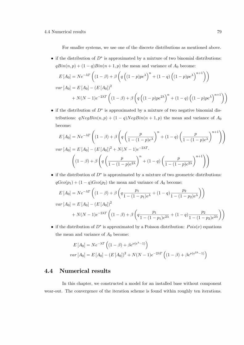
4.4 Numerical results 79
For smaller systems, we use one of the discrete distributions as mentioned above.
• if the distribution of D∗ is approximated by a mixture of two binomial distributions:qBin(n, p) + (1− q)Bin(n+ 1, p) the mean and variance of A0 become:
E [A0] = Ne−λT
µ(1− β) + β
µq³(1− p)peλ
´n+ (1− q)
³(1− p)peλ
´n+1¶¶var [A0] = E [A0]− (E [A0])2
+N(N − 1)e−2λTµ(1− β) + β
µq³(1− p)pe2λ
´n+ (1− q)
³(1− p)peλ
´n+1¶¶• if the distribution of D∗ is approximated by a mixture of two negative binomial dis-tributions: qNegBin(n, p) + (1 − q)NegBin(n + 1, p) the mean and variance of A0become:
E [A0] = Ne−λT
Ã(1− β) + β
Ãq
µp
1− (1− p)eλ
¶n+ (1− q)
µp
1− (1− p)eλ
¶n+1!!var [A0] = E [A0]− (E [A0])2 +N(N − 1)e−2λT ·Ã
(1− β) + β
Ãq
µp
1− (1− p)e2λ¶n+ (1− q)
µp
1− (1− p)e2λ¶n+1!!
• if the distribution of D∗ is approximated by a mixture of two geometric distributions:qGeo(p1) + (1− q)Geo(p2) the mean and variance of A0 become:
E [A0] = Ne−λT
µ(1− β) + β
µq
p11− (1− p1)eλ
+ (1− q) p21− (1− p2)eλ
¶¶var [A0] = E [A0]− (E [A0])2
+N(N − 1)e−2λTµ(1− β) + β
µq
p11− (1− p1)e2λ
+ (1− q) p21− (1− p2)e2λ
¶¶• if the distribution of D∗ is approximated by a Poisson distribution: Pois(ν) equationsthe mean and variance of A0 become:
E [A0] = Ne−λT
³(1− β) + βeν(e
λ−1)´
var [A0] = E [A0]− (E [A0])2 +N(N − 1)e−2λT³(1− β) + βeν(e
2λ−1)´
4.4 Numerical results
In this chapter, we constructed a model for an installed base without component
wear-out. The convergence of the iteration scheme is found within roughly ten iterations.
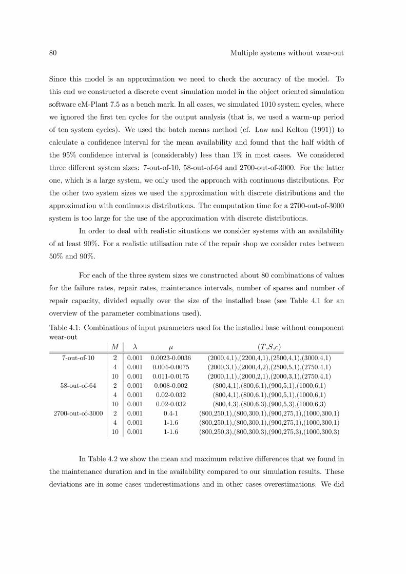
80 Multiple systems without wear-out
Since this model is an approximation we need to check the accuracy of the model. To
this end we constructed a discrete event simulation model in the object oriented simulation
software eM-Plant 7.5 as a bench mark. In all cases, we simulated 1010 system cycles, where
we ignored the first ten cycles for the output analysis (that is, we used a warm-up period
of ten system cycles). We used the batch means method (cf. Law and Kelton (1991)) to
calculate a confidence interval for the mean availability and found that the half width of
the 95% confidence interval is (considerably) less than 1% in most cases. We considered
three different system sizes: 7-out-of-10, 58-out-of-64 and 2700-out-of-3000. For the latter
one, which is a large system, we only used the approach with continuous distributions. For
the other two system sizes we used the approximation with discrete distributions and the
approximation with continuous distributions. The computation time for a 2700-out-of-3000
system is too large for the use of the approximation with discrete distributions.
In order to deal with realistic situations we consider systems with an availability
of at least 90%. For a realistic utilisation rate of the repair shop we consider rates between
50% and 90%.
For each of the three system sizes we constructed about 80 combinations of values
for the failure rates, repair rates, maintenance intervals, number of spares and number of
repair capacity, divided equally over the size of the installed base (see Table 4.1 for an
overview of the parameter combinations used).
Table 4.1: Combinations of input parameters used for the installed base without componentwear-out
M λ μ (T ,S,c)
7-out-of-10 2 0.001 0.0023-0.0036 (2000,4,1),(2200,4,1),(2500,4,1),(3000,4,1)4 0.001 0.004-0.0075 (2000,3,1),(2000,4,2),(2500,5,1),(2750,4,1)10 0.001 0.011-0.0175 (2000,1,1),(2000,2,1),(2000,3,1),(2750,4,1)
58-out-of-64 2 0.001 0.008-0.002 (800,4,1),(800,6,1),(900,5,1),(1000,6,1)4 0.001 0.02-0.032 (800,4,1),(800,6,1),(900,5,1),(1000,6,1)10 0.001 0.02-0.032 (800,4,3),(800,6,3),(900,5,3),(1000,6,3)
2700-out-of-3000 2 0.001 0.4-1 (800,250,1),(800,300,1),(900,275,1),(1000,300,1)4 0.001 1-1.6 (800,250,1),(800,300,1),(900,275,1),(1000,300,1)10 0.001 1-1.6 (800,250,3),(800,300,3),(900,275,3),(1000,300,3)
In Table 4.2 we show the mean and maximum relative differences that we found in
the maintenance duration and in the availability compared to our simulation results. These
deviations are in some cases underestimations and in other cases overestimations. We did
4.4 Numerical results 81
not find evidence that the approximation errors depend on the repair shop utilisation rate
or the system availability.
Table 4.2: Mean (max) differences between the approximations and the simulation resultsfor both the maintenance duration and the availability using the model with discrete dis-tributions and the model with continuous distributions
E[D] Av
discrete7-out-of-10 22.2% (106.7%) 1.4% (11.7%)58-out-of-64 3.5% (32.3%) 0.2% (2.1%)
2700-out-of-3000 - -continuous7-out-of-10 29.4% (111.6%) 1.6% (13.6%)58-out-of-64 4.0% (29.8%) 0.1% (0.6%)
2700-out-of-3000 3.5% (13.6%) 0.1% (0.5%)
For large systems we have no choice other than to use an approximation with
continuous distributions. Although the approximation of the maintenance duration may not
be very accurate at all times, we have a good approximation for the system availability. This
is due to the fact that the availability of the systems is 90% or more and the maintenance
duration is a relatively small part of the system’s cycle. As a result the impact of an error
in the maintenance duration is small.
For the medium sized systems we can choose between an approximation with
continuous or discrete distributions. If we would split the results according to the size of
the installed base we would see that for a larger installed base the approximation with
discrete distributions is slightly better than the one with continuous distributions.
In case of the small systems we find a better performance if we use the approxi-
mation with discrete distributions.
As seen in Table 4.2 the approximations for smaller systems are less satisfying.
This can be explained by the fact that an absolute small approximation error for Ai or Bi
is a relatively large error when we only have a few components. As a result, the error in the
approximation of the maintenance duration is relatively large. For systems with a larger
number of components the relative approximation errors are therefore smaller. Without
exception the maximum errors given in Table 4.2 are all generated by the scenarios with a
smaller size of the installed base.
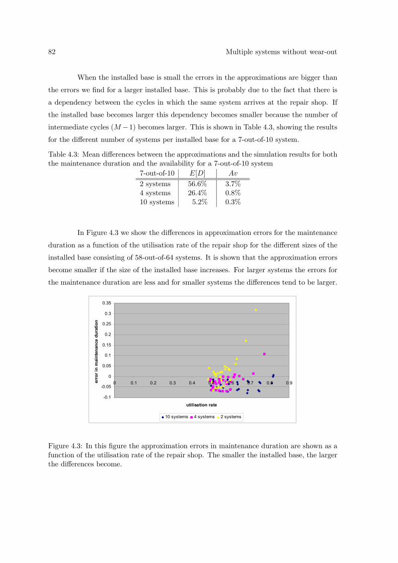
82 Multiple systems without wear-out
When the installed base is small the errors in the approximations are bigger than
the errors we find for a larger installed base. This is probably due to the fact that there is
a dependency between the cycles in which the same system arrives at the repair shop. If
the installed base becomes larger this dependency becomes smaller because the number of
intermediate cycles (M −1) becomes larger. This is shown in Table 4.3, showing the resultsfor the different number of systems per installed base for a 7-out-of-10 system.
Table 4.3: Mean differences between the approximations and the simulation results for boththe maintenance duration and the availability for a 7-out-of-10 system
7-out-of-10 E[D] Av
2 systems 56.6% 3.7%4 systems 26.4% 0.8%10 systems 5.2% 0.3%
In Figure 4.3 we show the differences in approximation errors for the maintenance
duration as a function of the utilisation rate of the repair shop for the different sizes of the
installed base consisting of 58-out-of-64 systems. It is shown that the approximation errors
become smaller if the size of the installed base increases. For larger systems the errors for
the maintenance duration are less and for smaller systems the differences tend to be larger.
-0.1
-0.05
0
0.05
0.1
0.15
0.2
0.25
0.3
0.35
0 0.1 0.2 0.3 0.4 0.5 0.6 0.7 0.8 0.9
utilisation rate
erro
r in
mai
nten
ance
dur
atio
n
10 systems 4 systems 2 systems
Figure 4.3: In this figure the approximation errors in maintenance duration are shown as afunction of the utilisation rate of the repair shop. The smaller the installed base, the largerthe differences become.
4.5 Conclusions 83
4.5 Conclusions
From the previous section we conclude that we have accurate approximations for
the availability as function of the maintenance interval, number of spare parts and the
number of repair capacity, provided that the number of components in a system is not too
small (a number of more than ten components seems to be sufficient) and the size of the
installed base is not too small (a number of at least four systems seems to be sufficient). We
can draw graphs in which we quantify the effect of the length of the maintenance interval
and the maintenance means (spares and capacity). Increasing the maintenance interval
means we can do with less spares or capacity (or both) and still have the same availability
performance. For systems with only a small number of components or a small installed base
we have to be careful because the approximation errors may be relatively large.

84 Multiple systems without wear-out
Chapter 5
Multiple systems with wear-out
In this chapter1 we model a wear-out process using three component states 0, 1
and 2 for a fully functional, degraded and failed component, respectively. We use the same
assumptions as in the previous chapter, given in Section 4.1 and
1. State transitions from state 0 to state 1 occur according to an exponential distribution
with rate λ1.
2. State transitions from state 1 to state 2 occur according to an exponential distribution
with rate λ2.
3. There are no direct transitions possible from state 0 to state 2.
4. During maintenance all degraded and failed components are replaced by spare com-
ponents.
5. The repair times for degraded and failed components are exponentially distributed
with rates μ1 and μ2 respectively.
To derive approximations for this model, we use an intermediate step, namely the
special case where the repair rates of degraded and failed components are identical, μ1 = μ2
(Section 5.1). Next, we address the variant where the repair rates may be different (Section
5.2). In the latter case, it makes a diference in which order we repair degraded and failed1This chapter is based on the paper: K.S. de Smidt-Destombes, M.C. van der Heijden and A. van Harten;
Spare parts analysis for k-out-of-N systems under block replacement and finite repair capacity; InternationalJournal of Production Economics ; to appear.
86 Multiple systems with wear-out
components because of the different repair rates, μ1 6= μ2. Hence, we use a scheduling rule
to decide in which order the spares are restored.
5.1 Equal repair rates: μ1 = μ2
If the repair rates of the degraded and failed components are equal, it is sufficient
to know the total number of components that are waiting or in repair at the start of a repair
cycle, which we define as B. The total number of failed and degraded components at the
start of a repair cycle equals B + A1 + A2 with Ai is the number of system components
in state i at system arrival in the repair shop (i = 0, 1, 2). Then our equation for the
maintenance duration (4.2) changes to:
D = R¡[B +A1 +A2 − S]+
¢= R
¡[B +N −A0 − S]+
¢(5.1)
Similar to the model without wear-out, the conditional distribution of the number
of components in state 0 at the start of a repair cycle given the length of the previous
maintenance time, A0|D, is binomial with parameters N and e−λ1(T−D). The unconditional
mean and variance of this stochastic variable are given by the equations 4.9 and 4.10 with
λ replaced by λ1.
The number of components that are not yet restored at the start of the repair
cycle B equals the number of spares to restore at the previous system arrival, plus the
failed components that came out of that system minus the number of repairs that is done
between the two system arrivals. Hence, we have the same equation as for the model without
wear-out, see equation 4.3 with A1 = N −A0.
B =
∙B +N −A0 − Z
µT
M
¶¸+(5.2)
Analogous to the model without ageing of components we use a moment iteration
method to solve this set of equations 5.1, 5.2 and 4.9 until 4.11. The generic iteration
scheme is as follows:
Step 0: initialisation, choose start values for E [A0], var [A0], E [B], var [B], E [D]
and var [D]. Approximate the mean and variance of Z¡TM
¢as in equations 4.7 and 4.8.
Step 1: determine the mean and variance of A0 using 4.9, 4.10 and 4.11.
5.1 Equal repair rates: μ1 = μ2 87
Step 2: find the mean and variance of Y = N −A0+B, assuming that A0 and B1are independent.
Step 3: find the mean and variance of B =£Y − Z
¡TM
¢¤+.
Step 4: find the mean and variance of X = [Y − S]+ after determining the meanand variance of Y = N −A0 +B again with the new values for the mean and variance for
B found in step 3.
Step 5: approximate the mean and variance of the maintenance duration D =
R(X) using the equations 4.5 and 4.6.
Step 6: convergence check: If the relative difference between the E [D] found in
this iteration and the previous one is smaller than some fixed ² then stop, else go to step 1.
In our model, we chose ² = 10−5.
In order to find the mean operational time E [U ], we also need the mean and
variance of eU , which changes because of the ageing of components. In De Smidt-Destombes,Van der Heijden and Van Harten (2006b) a recursive method is presented to find the first
two moments. In short, this method works as follows. We define T (i, j) as the time duration
to get from state (i, j) (state (i, j) refers to N − i− j components in state 0, i componentsin state 1 and j components in state 2) to a failed state which has N −k+1 components instate 2. This immediately gives us the starting values of the recursion, T (i,N − k+ 1) = 0and T 2(i,N − k + 1) = 0 for every value of 0 ≤ i ≤ k − 1. The recursion is given by:
E [T (i, j)] = τ(i, j) + α(i, j)E [T (i+ 1, j)] + β(i, j)E [T (i− 1, j + 1)]
E£T 2(i, j)
¤= 2τ(i, j)E [T (i, j)] + α(i, j)E
£T 2(i+ 1, j)
¤+ β(i, j)E
£T 2(i− 1, j + 1)
¤Here, τ(i, j) = 1
(N−i−j)λ1+iλ2 is defined as the expected sojourn time in state
(i, j), α(i, j) = (N−i−j)λ1(N−i−j)λ1+iλ2 is the probability of a transition from state 0 to state 1 and
β(i, j) = iλ2(N−i−j)λ1+iλ2 is the probability of a transition from state 1 to state 2. Now eU is
defined as the time from state (0, 0) to a failed state. Hence,
EheUi = E [T (0, 0)]
varheUi = E £T 2(0, 0)¤− (E [T (0, 0)])2
With the first two moments of eU and D, we are able to determine the expected
uptime U from equation 4.12.
88 Multiple systems with wear-out
5.2 Different repair rates: μ1 6= μ2
5.2.1 Repair strategy
We denote the repair rate for degraded and failed components by μ1 and μ2,
respectively. It is plausible that repair of failed components takes more time on average
than repair of degraded components, so μ1 ≥ μ2. The remainder of our analysis be based on
this assumption for ease of notation. It is straightforward to modify the analysis if μ2 > μ1.
If the two repair types (degraded and failed components) have different repair
rates, we can influence the maintenance duration and hence the availability by choosing
the order in which the repair jobs are processed. Hence we have an additional degree
of freedom, namely a repair priority rule that we can use to minimise the maintenance
duration. We know that we should recover exactly [B +A1 +A2 − S]+ components to
restore the system that arrived at the start of a repair cycle. Therefore, we have to choose
(a) how many of these [B +A1 +A2 − S]+ components should be degraded componentsand how many should be failed components (b) in which order we are going to repair these
[B +A1 +A2 − S]+ components. Regarding the first issue, it is obvious that we should
select as many degraded components as possible, because their repair rate is higher. If
we have insufficient degraded components, we add failed components until we reach the
required number of [B +A1 +A2 − S]+ components. Regarding the second issue, we canuse the fact that we can minimise the make span of a fixed set of repair jobs by selecting the
longest processing times first, see for instance Pinedo and Chao (1999). So, within the set
of degraded and failed components that we should repair to recover the system, we should
give priority to failed components. Summarised, our repair strategy is as follows:
If the number of degraded spares (state 1) is sufficient to replace all components in the
system, then only repair degraded ones. If the number of degraded spares is not sufficient,
start repairing the minimum number of failed components needed to repair the system and
next repair all degraded components.
During the time in which the repair shop repairs components without a direct
demand (the periods between maintenance periods in Figure 4.1) we want the repair shop
to restore as many spare parts as possible. Therefore, during this time the priority rule is:
First repair all degraded spares and then start repairing failed spares.
5.2 Different repair rates: μ1 6= μ2 89
Using these priority rules, we are able to define a set of equations, which is pre-
sented in Section 5.2.2.
5.2.2 Moment iteration scheme
The approach of the problem with ageing of components and different repair rates
is analogous to the one with distinguishing the components in state 1 and state 2. The
maintenance duration is therefore split into two parts, one part for the number of type 1
repairs and one part for the type 2 repairs. We defineW1 andW2 as stochastic variables for
the number of repairs of type 1 and repairs of type 2 respectively during the maintenance
time. Then, we approximate the expected maintenance duration and its variance by:
E [D] ≈ E [W1]
cμ1+E [W2]
cμ2(5.3)
var [D] ≈ E [W1] + var [W1]
(cμ1)2
+E [W2] + var [W2]
(cμ2)2
(5.4)
To determine the workload of type 1 and type 2 we use the priority rule as discussed
in the previous section. This implies the workload of type 2 components to be zero as long
as the total number of failed components, A2 + B2, is at most equal to S. Otherwise the
workload is equal to the difference between the total number of failed components and the
number of spares.
W2 = [A2 +B2 − S]+ (5.5)
For the workload of type 1 components we consider the total workload and subtract
the workload of type 2 components. The total number of degraded and failed components
in the system and the repair shop equals A1+A2+B1+B2 = N −A0+B1+B2. The totalworkload is the total number of degraded and failed components minus the number that
does not need to be restored during the system maintenance period. In other words, if the
total number of components to restore is less than or equal to S, the total workload during
maintenance is zero, otherwise the workload is the difference between the components to
restore and S. Hence, we find for the workload of type 1 and type 2 components:
W1 = [N −A0 +B1 +B2 − S]+ −W2 (5.6)
90 Multiple systems with wear-out
Because of the different repair rates, we split up the number of unrepaired spares
B into B1 and B2 where Bi denotes the number of components in state i in the repair shop
at arrival of a system. The number of spare components in state 1 is equal to the total
number of components in state 1 just after the previous system arrival (B1+A1) minus the
number of repairs done in the time left after the W2 type 2 repairs. For B2, we assume that
W2 is repaired before the next system arrives. This is a reasonable assumption since these
are the first components to be restored and the availability requirements of the systems are
rather high. Then B2 equals the total number of components in state 2 minus W2 minus
the number of restores done in the time left after W2 and B1 + A1 are repaired. We then
find the following equations for Bi:
B0 = [S −B1 −B2]+ (5.7)
B1 =
"B1 +A1 − Z1
Ã∙T
M−R2(W2)
¸+!#+(5.8)
B2 =
"B2 +A2 −W2 − Z2
Ã∙T
M−R2(W2)−R1(A1 +B1)
¸+!#+(5.9)
Here Ri(X) is defined as the time needed to restore X components of type i
and Zi(X) is defined as the number of repairs of type i during X. If we use a moment
iteration scheme to determine the maintenance duration using equations 5.3 until 5.9 the
results are not very good. In the expression for W1, we have a correlation between the
total workload during maintenance and the workload of type 2 components that we ignore
in our approximations. This affects the variance of W1 and consequently also affects the
variance of D. The simulations, that we describe in more detail in Section 5.3, show that
this correlation is often close to 1. For the approximation of B2 we have a correlation
between W2 and A2 + B2 which is at least 0.6 according to our simulation. To deal with
these problems, we can try to estimate the magnitude of the correlations. Unfortunately,
this is mathematically hard. As an alternative, we can reformulate equations 5.3 until 5.9
in terms of other random variables, such that the correlations are less severe. Below, we
derive such alternative expressions for W1 and B2.
Regarding W1 we know that if the maintenance duration equals zero, then the
value of W1 equals zero. The probability that the maintenance duration is larger than zero,
is Pr (A1 +A2 +B1 +B2 > S) = Pr (N −A0 +B1 +B2 > S) = β. The total number of
5.2 Different repair rates: μ1 6= μ2 91
spares to restore during the maintenance period is N−A0+B1+B2−S, under the conditionthat N −A0 +B1 +B2 − S > 0. The time needed to restore this number of spares equalsD∗. Now there are two possibilities. The first possibility is that we need to restore only
part of the components in state 1. Then the value of W1 becomes equal to the number of
restores that can be done during D∗, Z1(D∗). The second possibility is that we need to
restore all components in state 1 and maybe even a number of components in state 2. The
value of W1 is then equal to A1 +B1. Combining these different possibilities we find:
W1 = min Z1(D∗), A1 +B1β + 0(1− β) (5.10)
Regarding B2, we add the assumption that we are also able to restore all type 1
components, A1+B1, before the next system arrives in the repair shop. This assumption is
not an unreasonable one as long as we are dealing with utilisation rates of the repair shop
that are not too large, say 90% to 95%. Hence, we approximate B2 by using the following
expression:
B2 =
"B2 +A2 − Z2
Ã∙T
M−R1(A1 +B1)
¸+!#+(5.11)
For the mean and variance of A0 we use the previous expressions 4.9 and 4.10.
The number of components in state 1 also has a binomial distribution with parameters N
and λ1λ1−λ2
¡e−λ2(T−D) − e−λ1(T−D)
¢and the number of components in state 2 is binomially
distributed with parameters N and 1− e−λ1(T−D) − λ1λ1−λ2
¡e−λ2(T−D) − e−λ1(T−D)
¢. With
some algebra we find:
E [A1] = Nλ1
λ1 − λ2
³e−λ2TE
heλ2D
i− e−λ1TE
heλ1D
i´(5.12)
var [A1] = (N2 −N)
µλ1
λ1 − λ2
¶2 ³e−2λ2TE
he2λ2D
i− 2e−(λ1+λ2)TE
he(λ1+λ2)D
i(5.13)
+e−2λ1TEhe2λ1D
i´+E [A1]− (E [A1])2
E [A2] = N −E [A0]−E [A1] (5.14)
var [A2] =2N(N − 1)λ1
λ1 − λ2
³e−(λ1+λ2)TE
he(λ1+λ2)D
i− e−2λ1TE
he2λ1D
i´(5.15)
+ var [A0] + var [A1]− 2E [A0]E [A1]
92 Multiple systems with wear-out
To find an approximation of the maintenance duration we use a moment iteration
method using equations 5.3 until 5.5, 5.7, 5.8, 5.10 until 5.15, 4.9 and 4.10. The iteration
scheme becomes as follows.
Step 0: initialisation, choose start values for E [A0], var [A0], E [B0], var [B0],
E [W2], var [W2], E [D] and var [D].
Step 1: determine the means and variances ofA0 (using equations 4.9 and 4.10) and
A1 and A2 using equations 5.12 until 5.15. Therefore, we take out the point mass ofD in zero
and use equation 4.11 with β = Pr (A1 +A2 +B1 +B2 > S) = Pr (N −A0 +B1 +B2 > S).Step 2: find the mean and variance of B1 = [B1 +A1 − Z1(X)]+ with X =£
TM −R2(W2)
¤+. Therefore we first determine the mean and variance of R2(W2) using equa-
tions 4.5 and 4.6 with μ replaced by μ2 andX =W2. Secondly we find the mean and variance
of the time available for type 2 repairs during a repair shop cycle: X =£TM −R2(W2)
¤+.
Thirdly, we find the mean and variance of Z1(X) using the approximations given in equa-
tions 4.7 and 4.8 with μ replaced by μ1. Finally we find the mean and variance of B1.
Step 3: find the mean and variance of B2 = [B2 +A2 − Z2(Y )]+ with Y =£TM −R1(A1 +B1)
¤+. Therefore we first find the mean and variance of R1(A1 + B1) ap-
proximated by equations 4.5 and 4.8 with X = A1+B1 and μ replaced by μ1. Secondly we
find the mean and variance of Y and thirdly we find the mean and variance of Z2(Y ) using
the approximations given in equations 4.7 and 4.8 with μ replaced by μ2. Finally, we find
the mean and variance of B2.
Step 4: find the mean and variance of B0 = [S −B1 −B2]+.Step 5: find the mean and variance of W1 =
¡A1 +B1 − [A1 +B1 − Z1(D∗)]+
¢β
with β as found in step 1 and the mean and variance of Z1(D∗), with the mean and variance
of D∗ as we found in step 1 to take out the point mass.
Step 6: find the mean and variance of W2 = [A2 +B2 − S]+.Step 7: approximate the mean and variance of the maintenance duration using
the equation 5.3 for E [D] and equation 5.4 for var [D] :
Step 8: convergence check. If the relative difference between the E [D] found in
this iteration and the previous one is smaller than some fixed ² then stop, else go to step 1.
In our model we chose ² = 10−5.
To compute the mean operational time for the systems E [U ] we use the same
method as described in the model with ageing of components and equal repair rates.
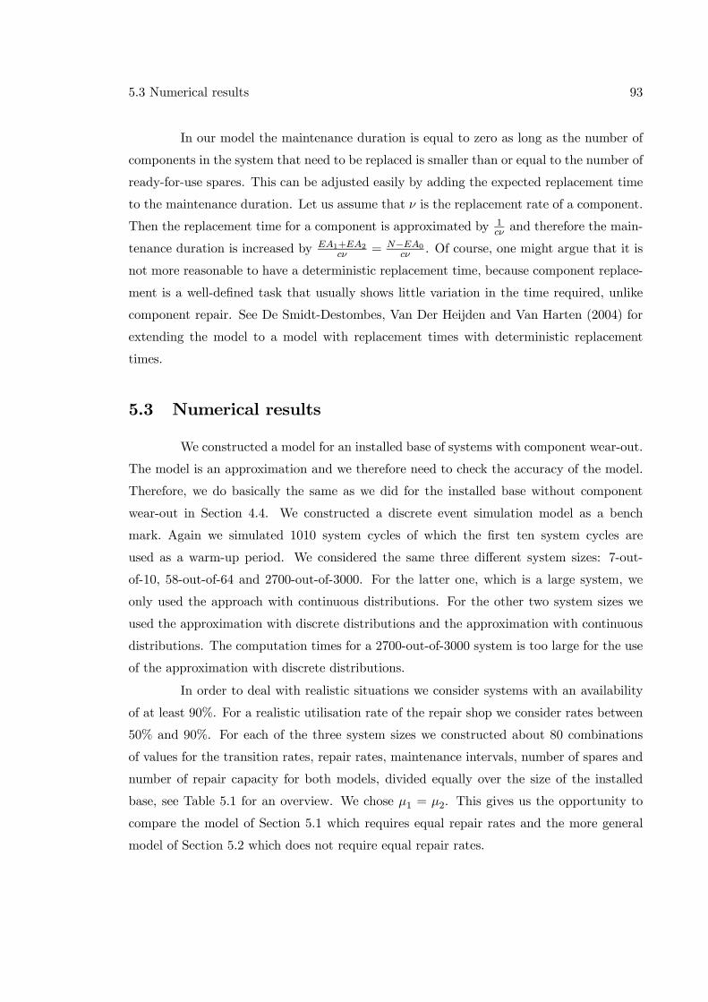
5.3 Numerical results 93
In our model the maintenance duration is equal to zero as long as the number of
components in the system that need to be replaced is smaller than or equal to the number of
ready-for-use spares. This can be adjusted easily by adding the expected replacement time
to the maintenance duration. Let us assume that ν is the replacement rate of a component.
Then the replacement time for a component is approximated by 1cν and therefore the main-
tenance duration is increased by EA1+EA2cν = N−EA0
cν . Of course, one might argue that it is
not more reasonable to have a deterministic replacement time, because component replace-
ment is a well-defined task that usually shows little variation in the time required, unlike
component repair. See De Smidt-Destombes, Van Der Heijden and Van Harten (2004) for
extending the model to a model with replacement times with deterministic replacement
times.
5.3 Numerical results
We constructed a model for an installed base of systems with component wear-out.
The model is an approximation and we therefore need to check the accuracy of the model.
Therefore, we do basically the same as we did for the installed base without component
wear-out in Section 4.4. We constructed a discrete event simulation model as a bench
mark. Again we simulated 1010 system cycles of which the first ten system cycles are
used as a warm-up period. We considered the same three different system sizes: 7-out-
of-10, 58-out-of-64 and 2700-out-of-3000. For the latter one, which is a large system, we
only used the approach with continuous distributions. For the other two system sizes we
used the approximation with discrete distributions and the approximation with continuous
distributions. The computation times for a 2700-out-of-3000 system is too large for the use
of the approximation with discrete distributions.
In order to deal with realistic situations we consider systems with an availability
of at least 90%. For a realistic utilisation rate of the repair shop we consider rates between
50% and 90%. For each of the three system sizes we constructed about 80 combinations
of values for the transition rates, repair rates, maintenance intervals, number of spares and
number of repair capacity for both models, divided equally over the size of the installed
base, see Table 5.1 for an overview. We chose μ1 = μ2. This gives us the opportunity to
compare the model of Section 5.1 which requires equal repair rates and the more general
model of Section 5.2 which does not require equal repair rates.
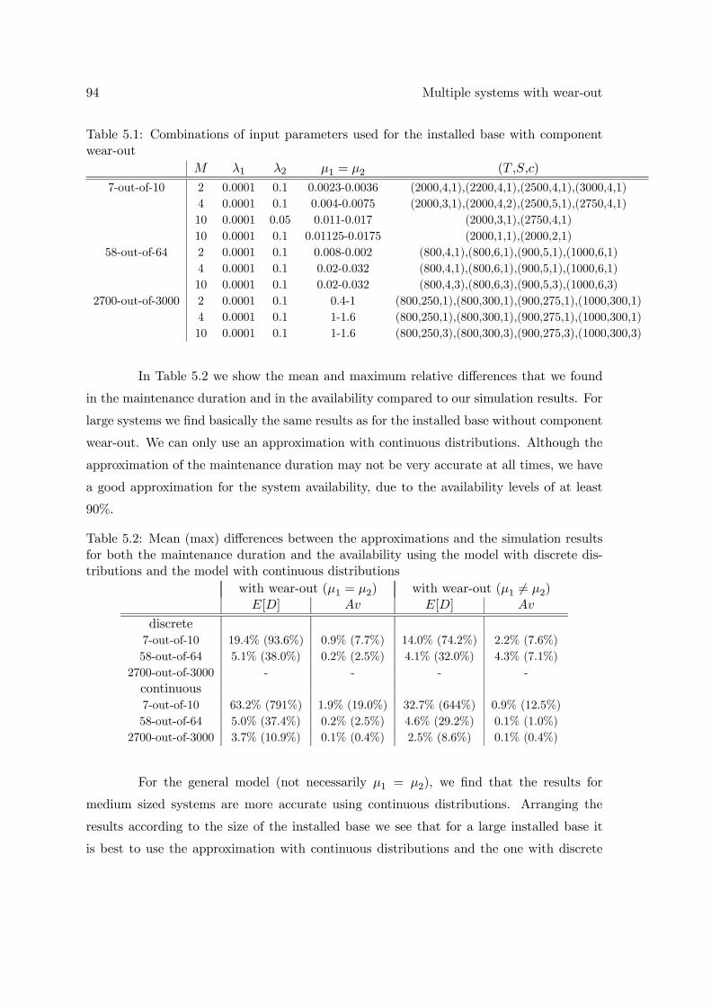
94 Multiple systems with wear-out
Table 5.1: Combinations of input parameters used for the installed base with componentwear-out
M λ1 λ2 μ1 = μ2 (T ,S,c)
7-out-of-10 2 0.0001 0.1 0.0023-0.0036 (2000,4,1),(2200,4,1),(2500,4,1),(3000,4,1)4 0.0001 0.1 0.004-0.0075 (2000,3,1),(2000,4,2),(2500,5,1),(2750,4,1)10 0.0001 0.05 0.011-0.017 (2000,3,1),(2750,4,1)10 0.0001 0.1 0.01125-0.0175 (2000,1,1),(2000,2,1)
58-out-of-64 2 0.0001 0.1 0.008-0.002 (800,4,1),(800,6,1),(900,5,1),(1000,6,1)4 0.0001 0.1 0.02-0.032 (800,4,1),(800,6,1),(900,5,1),(1000,6,1)10 0.0001 0.1 0.02-0.032 (800,4,3),(800,6,3),(900,5,3),(1000,6,3)
2700-out-of-3000 2 0.0001 0.1 0.4-1 (800,250,1),(800,300,1),(900,275,1),(1000,300,1)4 0.0001 0.1 1-1.6 (800,250,1),(800,300,1),(900,275,1),(1000,300,1)10 0.0001 0.1 1-1.6 (800,250,3),(800,300,3),(900,275,3),(1000,300,3)
In Table 5.2 we show the mean and maximum relative differences that we found
in the maintenance duration and in the availability compared to our simulation results. For
large systems we find basically the same results as for the installed base without component
wear-out. We can only use an approximation with continuous distributions. Although the
approximation of the maintenance duration may not be very accurate at all times, we have
a good approximation for the system availability, due to the availability levels of at least
90%.
Table 5.2: Mean (max) differences between the approximations and the simulation resultsfor both the maintenance duration and the availability using the model with discrete dis-tributions and the model with continuous distributions
with wear-out (μ1 = μ2) with wear-out (μ1 6= μ2)E[D] Av E[D] Av
discrete7-out-of-10 19.4% (93.6%) 0.9% (7.7%) 14.0% (74.2%) 2.2% (7.6%)58-out-of-64 5.1% (38.0%) 0.2% (2.5%) 4.1% (32.0%) 4.3% (7.1%)
2700-out-of-3000 - - - -continuous7-out-of-10 63.2% (791%) 1.9% (19.0%) 32.7% (644%) 0.9% (12.5%)58-out-of-64 5.0% (37.4%) 0.2% (2.5%) 4.6% (29.2%) 0.1% (1.0%)
2700-out-of-3000 3.7% (10.9%) 0.1% (0.4%) 2.5% (8.6%) 0.1% (0.4%)
For the general model (not necessarily μ1 = μ2), we find that the results for
medium sized systems are more accurate using continuous distributions. Arranging the
results according to the size of the installed base we see that for a large installed base it
is best to use the approximation with continuous distributions and the one with discrete
5.3 Numerical results 95
distributions for the smaller sizes of the installed base.
Again, we see in Table 5.2 that the approximations for smaller systems are less
good. This is explained by the few number of components. Without exception the maximum
errors given in Table 5.2 are all generated by the scenarios with a smaller size of the installed
base. Also, when the installed base is small the errors in the approximations are much
worse than the errors we find for a larger installed base. This is caused by the fact that the
dependency between the cycles becomes smaller if the installed base becomes larger. This
is shown in Table 5.3, showing the results for the different number of systems per installed
base for a 7-out-of-10 system.
For the systems with component wear-out the approximation errors for the main-
tenance duration as a function of the utilisation rate of the repair shop shows the same
pattern as for the systems without component wear-out. See Figure 4.3 which shows the
differences in approximation errors for maintenance duration as a function of the utilisation
rate of the repair shop for the different sizes of the installed base consisting of 58-out-of-64
systems. The approximation errors become smaller if the size of the installed base increases.
Again, for larger systems the errors for the maintenance duration are less and for smaller
systems the differences become larger.
Table 5.3: Mean differences between the approximations and the simulation results for boththe maintenance duration and the availability for a 7-out-of-10 system
with wear-out (μ1 = μ2) with wear-out (μ1 6= μ2)7-out-of-10 E[D] Av E[D] Av
2 systems 42.3% 2.0% 25.0% 1.3%4 systems 13.7% 0.5% 11.9% 3.2%10 systems 3.8% 0.2% 5.0% 2.2%
Looking at Table 5.2 again there is an other interesting result. When we look at
the approximation errors for the maintenance duration for the two models we see that the
model that does not require the repair rates μ1 and μ2 to be equal to give less satisfactorily
approximations. While for the same scenarios we find that for the approximations of the
availability the results are the other way around. The scenarios in which this happens are
scenarios with either a small installed base or an availability level of over 99%. For the
scenarios with a small installed base we already concluded that the model does not perform
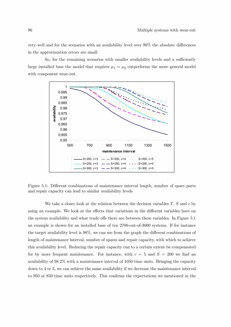
96 Multiple systems with wear-out
very well and for the scenarios with an availability level over 99% the absolute differences
in the approximation errors are small.
So, for the remaining scenarios with smaller availability levels and a sufficiently
large installed base the model that requires μ1 = μ2 outperforms the more general model
with component wear-out.
0.950.955
0.960.965
0.970.975
0.980.985
0.990.995
1
500 700 900 1100 1300 1500
maintenance interval
avai
labi
lity
S=200, c=3 S=200, c=4 S=200, c=5S=250, c=3 S=250, c=4 S=250, c=5S=300, c=3 S=300, c=4 S=300, c=5
Figure 5.1: Different combinations of maintenance interval length, number of spare partsand repair capacity can lead to similar availability levels
We take a closer look at the relation between the decision variables T , S and c by
using an example. We look at the effects that variations in the different variables have on
the system availability and what trade offs there are between these variables. In Figure 5.1
an example is shown for an installed base of ten 2700-out-of-3000 systems. If for instance
the target availability level is 98%, we can see from the graph the different combinations of
length of maintenance interval, number of spares and repair capacity, with which to achieve
this availability level. Reducing the repair capacity can to a certain extent be compensated
for by more frequent maintenance. For instance, with c = 5 and S = 200 we find an
availability of 98.2% with a maintenance interval of 1050 time units. Bringing the capacity
down to 4 or 3, we can achieve the same availability if we decrease the maintenance interval
to 950 or 850 time units respectively. This confirms the expectations we mentioned in the
5.4 Conclusions 97
introduction of this paper that a higher maintenance frequency of leads to less variation
in the component arrival process at the repair shop, so that less repair capacity is needed.
For the number of spares we see similar results. Looking at it the other way around we
see that with an increase of the spares from 200 to 300 we can increase our maintenance
interval from 650 to 1100 and still have an availability of almost 99.5% with c = 3. So,
with a decreasing maintenance interval we can decrease the repair capacity, decrease the
number of spares or decrease both. With this model the effects can be made quantitative
for specific cases. Which combination of parameters (T , S, c) is the best, depends on the
cost involved. Without loss of performance the cheapest option can be chosen.
5.4 Conclusions
The conclusions for the model for an installed base of systems with component
wear-out as we described in this chapter are not very different from the ones for the model
for an installed base of systems without component wear-out. As long as the system size
is not too small, roughly more than 10 components, and the installed base is sufficiently
large, at least 4, we have accurate approximations for the availability as function of the
maintenance interval, spare parts and repair capacity.
Given the approximations as provided in this chapter, we are not able to find the
optimal combination of maintenance interval, number of spares and repair capacity with
respect to costs. Given the number of combinations for the decision variables and the
computation times, enumeration is usually not an option. Therefore, the development of
an optimisation method is the subject of the next chapter.

98 Multiple systems with wear-out
Chapter 6
Optimisation algorithms
In the previous chapters we developed mathematical models in order to compute
the operational availability as a function of the maintenance frequency, the number of spare
parts and the repair capacity. Various combinations of these three parameters lead to similar
availability levels at different costs levels. In this chapter we concentrate on finding the cost
optimal parameter setting such that a target system availability is attained. In Section
6.1 we discuss briefly the optimisation methods we found in the literature for these type
of problems. In Sections 6.2 and 6.3 we explain the optimisation methods we developed
for respectively the single system and an installed base including numerical results. We
illustrate our optimisation heuristic using a case study (a part of the Anaconda) in Section
6.4. We end this chapter with some conclusions in Section 6.5.
6.1 Introduction
We can use the models that we developed in the previous sections as a basis for
an optimisation method. However, this is not straightforward, since we are dealing with a
non-linear, integer optimisation problem under a nonlinear restriction as we explain in the
subsequent sections. In the literature, various approaches to tackle such a problem have
been described. In a series of papers by Wang (Wang (1995), Wang and Wu (1995), Wang
(1994a), Wang (1994b), Wang (1993)) different models with redundant components and
spares are considered and for every model a direct search heuristic is used. In the papers,
it is stated that this direct search approach is performed over a grid whose boundaries for
decision variables are selected in order to guarantee that the optimum is obtained in the
100 Optimisation algorithms
interior region. This suggests that enumeration is used, and is therefore less applicable
for our problem. Sherbrooke (1968) shows that the determination of inventory levels in
multi-echelon, multi-indenture networks can be done by using another heuristic, a marginal
analysis called METRIC. He addresses the problem of maximising the average availability
of an installed base of systems under a budget restriction on the total spare part investment.
Decision variables are the stock levels of all repairable items that may be replaced on failure,
at all locations in a multi-echelon network. Sherbrooke (1968) shows that maximising
availability is approximately equivalent to minimise the sum of the expected backorders of
all main assemblies at all downstream locations. Starting from some initial inventory levels
(that may be zero), the heuristic subsequently adds an item to stock at a specific location
that yields the highest decrease in expected backorders per invested Euro. Sleptchenko
(2002) shows that this heuristic can be extended to a model for simultaneous optimisation
of spare parts inventory levels and repair capacity for spare parts. Because it turns out that
the costs as function of the number of spare parts and capacity are not always convex, the
author uses initial values for the number of spares larger than zero, a non-integer number
of servers and a technique for balancing the availability over the different locations in the
system.
A further extension of the model by including the maintenance frequency leads to
an additional complication because the availability might not be a monotonous function of
the maintenance frequency. When the frequency decreases, the probability that the system
fails before maintenance starts increases and this pushes the availability down. On the other
hand, the cycle length increases and the expected uptime in a cycle increases as well, which
pushes the availability up. The aggregate effect may both be a decrease and an increase in
the system availability. This effect was noticeable in all models as discussed in the previous
chapters.
The remark above indicates that the development of a joint optimisation method
for spare part inventories, repair capacity and maintenance frequency is not straightforward.
In this chapter we develop two optimisation methods, one for the single system (see the
model described in Chapter 2 and Chapter 3) and one for the installed base (see Chapter 4
and Chapter 5). We consider the following cost categories:
• The holding and depreciation costs of a spare per time unit, Cspare
• The cost of repair capacity per time unit, Ccapacity
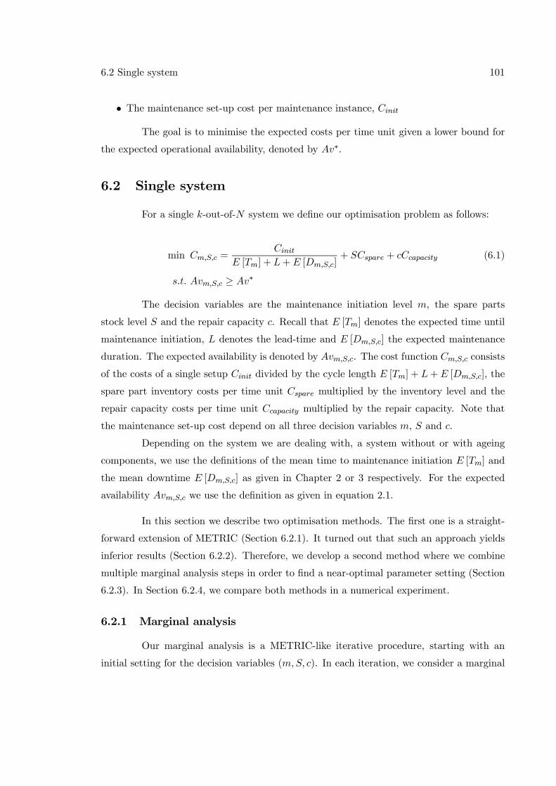
6.2 Single system 101
• The maintenance set-up cost per maintenance instance, Cinit
The goal is to minimise the expected costs per time unit given a lower bound for
the expected operational availability, denoted by Av∗.
6.2 Single system
For a single k-out-of-N system we define our optimisation problem as follows:
min Cm,S,c =Cinit
E [Tm] + L+E [Dm,S,c]+ SCspare + cCcapacity (6.1)
s.t. Avm,S,c ≥ Av∗
The decision variables are the maintenance initiation level m, the spare parts
stock level S and the repair capacity c. Recall that E [Tm] denotes the expected time until
maintenance initiation, L denotes the lead-time and E [Dm,S,c] the expected maintenance
duration. The expected availability is denoted by Avm,S,c. The cost function Cm,S,c consists
of the costs of a single setup Cinit divided by the cycle length E [Tm] + L+E [Dm,S,c], the
spare part inventory costs per time unit Cspare multiplied by the inventory level and the
repair capacity costs per time unit Ccapacity multiplied by the repair capacity. Note that
the maintenance set-up cost depend on all three decision variables m, S and c.
Depending on the system we are dealing with, a system without or with ageing
components, we use the definitions of the mean time to maintenance initiation E [Tm] and
the mean downtime E [Dm,S,c] as given in Chapter 2 or 3 respectively. For the expected
availability Avm,S,c we use the definition as given in equation 2.1.
In this section we describe two optimisation methods. The first one is a straight-
forward extension of METRIC (Section 6.2.1). It turned out that such an approach yields
inferior results (Section 6.2.2). Therefore, we develop a second method where we combine
multiple marginal analysis steps in order to find a near-optimal parameter setting (Section
6.2.3). In Section 6.2.4, we compare both methods in a numerical experiment.
6.2.1 Marginal analysis
Our marginal analysis is a METRIC-like iterative procedure, starting with an
initial setting for the decision variables (m,S, c). In each iteration, we consider a marginal
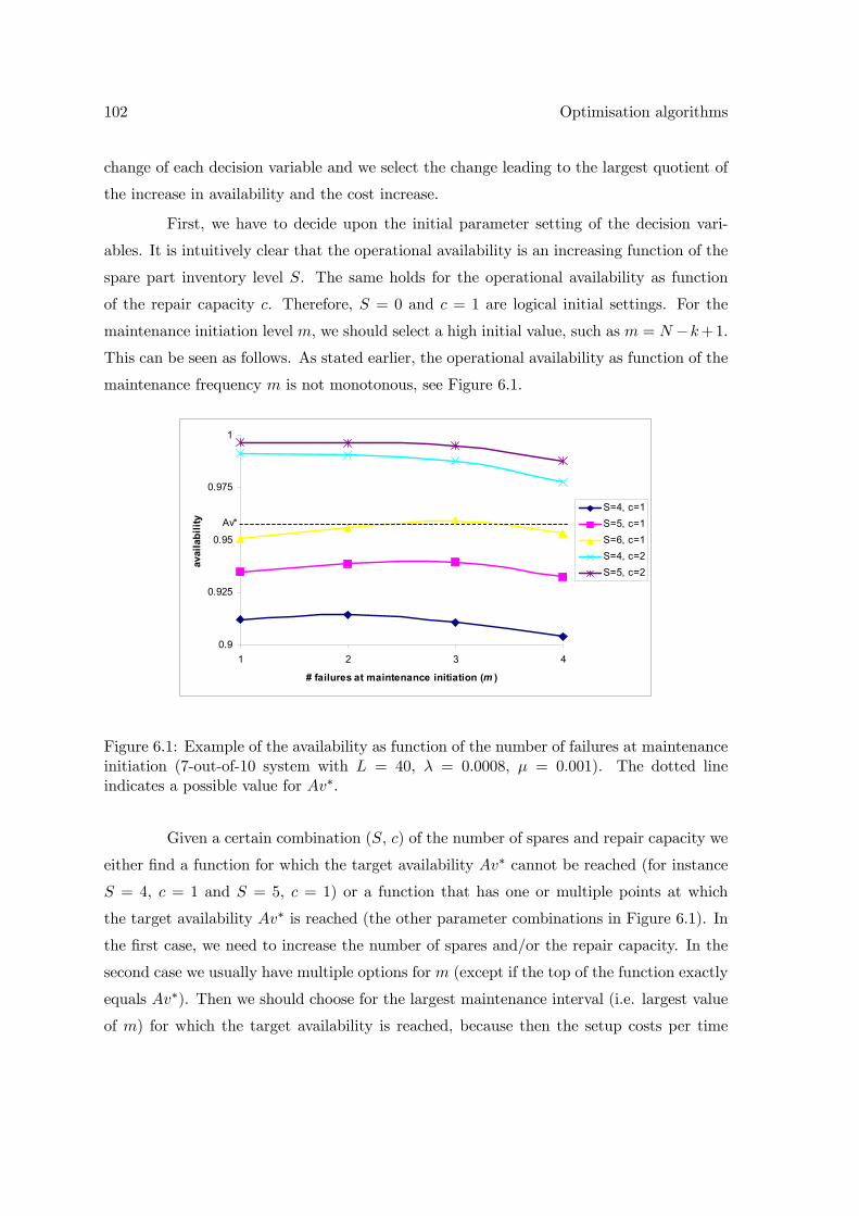
102 Optimisation algorithms
change of each decision variable and we select the change leading to the largest quotient of
the increase in availability and the cost increase.
First, we have to decide upon the initial parameter setting of the decision vari-
ables. It is intuitively clear that the operational availability is an increasing function of the
spare part inventory level S. The same holds for the operational availability as function
of the repair capacity c. Therefore, S = 0 and c = 1 are logical initial settings. For the
maintenance initiation level m, we should select a high initial value, such as m = N −k+1.This can be seen as follows. As stated earlier, the operational availability as function of the
maintenance frequency m is not monotonous, see Figure 6.1.
0.9
0.925
0.95
0.975
1
1 2 3 4
# failures at maintenance initiation (m )
avai
labi
lity
S=4, c=1S=5, c=1S=6, c=1S=4, c=2S=5, c=2
Av*
Figure 6.1: Example of the availability as function of the number of failures at maintenanceinitiation (7-out-of-10 system with L = 40, λ = 0.0008, μ = 0.001). The dotted lineindicates a possible value for Av∗.
Given a certain combination (S, c) of the number of spares and repair capacity we
either find a function for which the target availability Av∗ cannot be reached (for instance
S = 4, c = 1 and S = 5, c = 1) or a function that has one or multiple points at which
the target availability Av∗ is reached (the other parameter combinations in Figure 6.1). In
the first case, we need to increase the number of spares and/or the repair capacity. In the
second case we usually have multiple options for m (except if the top of the function exactly
equals Av∗). Then we should choose for the largest maintenance interval (i.e. largest value
of m) for which the target availability is reached, because then the setup costs per time
6.2 Single system 103
unit are lowest (the maintenance interval and so the cycle length is higher). We therefore
start our marginal analysis with the largest realistic value for m and consider the option
of decreasing m by one. Then the maintenance frequency and hence the setup costs per
time unit increases, whereas the availability may both increase or decrease, as we see from
Figure 6.1. If the availability decreases then decreasing the value of m is not an option (we
would have a lower availability level against higher costs).
As high initial value of m, it is logical to choose m = N − k+1 at first sight. Anychoice m > N −k+1 is useless, because then we force unnecessary downtime. It is howeverpossible that for the large values of m the target availability cannot be reached, simply
because we get too much down time during the lead-time L. This is solely influenced by m
and cannot be compensated by adding spares or repair capacity, see equation 2.2. Therefore,
a tighter upper bound form is the value for which we are able to reach the target availability
Av∗ if the maintenance duration would be zero (this is independent of the values of S and
c). This results in the upper limit mmax :
mmax = max
½1 ≤ m ≤ N − k + 1
¯E [Tm] +E [Um]
E [Tm] + L≥ Av∗
¾(6.2)
where Um denotes the uptime during the lead time L if maintenance is initiated
when m components have failed. We conclude that the initial setting of our decision vari-
ables should be given by S = 0, c = 1 and m = mmax.
Next, as a straightforward extension of METRIC, we consider decreasing m, in-
creasing S and increasing c in each step of the algorithm. We select the option that yields
the highest increase in availability relative to the additional investment (i.e., setup costs,
spare costs or repair costs per time unit). We just use one additional modification. While
performing the algorithm, we may either encounter one or more options for which Av ≥ Av∗
and another option with the largest increment of the availability per cost unit andAv < Av∗.
By default, we select the latter option and move to the next iteration. However, it is pos-
sible that one of the first options turns out to be cheaper after all. Therefore, we store the
cheapest parameter setting satisfying Av ≥ Av∗ that we encounter during the execution
of the algorithm. If this alternative is better than the solution found with the standard
marginal analysis, we take the first option as the final solution. Although this modification
seems to be marginal, it improves the performance of our algorithm as we observed in our
preliminary numerical experiments. Summarising, the marginal analysis algorithm consists
104 Optimisation algorithms
of the following steps:
Step 1 : Initialise S = 0, c = 1 and m = mmax
Determine Avm,S,c and Cm,S,c.
Step 2a : Determine Avm−1,S,c, Avm,S+1,c and Avm,S,c+1.
Determine Cm−1,S,c, Cm,S+1,c and Cm,S,c+1.
Step 2b : Choose parameter setting (x, y, z) ∈ (m− 1, S, c), (m,S + 1, c), (m,S, c+ 1)where Avx,y,z−Avm,S,c
Cx,y,z−Cm,S,c is maximal.
Step 3a : If one or more parameter settings yield Av ≥ Av∗, then store the cheapest.Step 3b : Choose (m,S, c) = (x, y, z), Avm,S,c = Avx,y,z and Cm,S,c = Cx,y,z.
If Avm,S,c < Av∗ then go to Step 2a else go to Step 4 .
Step 4 : Choose the cheapest parameter setting from Step 2b and Step 3a.
Unfortunately, the numerical experiments (that we discuss in more detail in Section
6.2.4) revealed that this algorithm may yield solutions that are far from optimal. Depending
on the number of components in the system, we find significant deviations from the true
optimum as found by enumeration. A cost difference of 10-20% is not uncommon and the
worst case is even a deviation of 171%! In the next section, we analyse the causes of this
problem. Next, we develop an alternative heuristic that avoids local optima that are much
worse than the global optimum.
6.2.2 Drawbacks marginal analysis
The key cause for the bad performance of the marginal analysis from the previous
section is the non-convexity of the function of expected costs Cm,S,c and the expected
availability Avm,S,c in the decision variables m, c and S. We distinguish four major issues
that oppose a good performance of the marginal analysis algorithm:
1. step size of the repair capacity c
2. choice of the initial parameter setting in the algorithm
3. shape of the availability as function of the maintenance initiation level m
4. overestimation of either spares S or repair capacity c
6.2 Single system 105
The first issue arises from the large impact of an increase in repair capacity on both
costs and availability if the repair shop capacity c is small and the repair shop utilisation is
high. For example, suppose that we have a repair shop utilisation of 0.95 when c = 1. An
increase to c = 2 means a decrease in utilisation to 0.475, which has an enormous impact on
the repair shop throughput times. Such an effect can hardly be called ”marginal”. Besides,
it is plausible that an optimal repair shop utilisation may be around 0.6− 0.8, which valuesare not even considered in this example. We can solve this problem by allowing c to have
non-integer values (see Sleptchenko (2002)). For practical purposes we can interpret this as
e.g. part time work or overtime. Then we can use a step size of (for example) 0.1 full time
equivalent (fte) instead of 1 fte. Similarly, we can also choose for only integer values of c
and decrease the repair rate with a factor of ten as well as the cost for capacity, so that
the minimum capacity is (for example) c = 10. In the next subsection, we discuss how this
minimum capacity can be computed.
The second issue, concerning the initial values of the parameters, is encountered if
the number of spares is small, say far less than the expected number of spares that is needed
for replacement during maintenance. In this case the amount of spares is far insufficient
and the marginal impact of an extra spare on the availability may be small. Consequently,
it is not likely that the marginal analysis will choose adding an extra spare. Instead, we see
an increase in repair capacity c or a decrease of m. However, when the number of spares
would have been larger, the marginal impact on the availability would be higher and so it
would be attractive to buy more spares. Therefore, we may conclude that the availability
is non convex in the number of spares.
In order to tackle this non convexity issue, Rustenburg (2000) suggests starting
values for the number of spares. These starting values are related to the average number
of spares in the pipeline at the time of a spare demand. In fact, it means that the starting
values are such that the safety stocks are approximately zero. It is plausible that the optimal
safety stocks will usually be nonnegative. In our model, zero safety stock would mean a
number of spares equal to the expected number of failed components in the system when
maintenance starts. This means that we only have spare parts available for the expected
demand and that our safety stock is zero. However, the corresponding stock level S increases
in the maintenance initiation level m (assuming c to be constant). So the initial value of S
depends on m = mmax, and when m decreases during the execution of the algorithm, the
106 Optimisation algorithms
current value of S can be above the initial level for the new value of m. As a consequence,
S can have a value above the new initial stock level, even if no spares have been added
during the course of the algorithm, and therefore S can be higher than the optimal level,
as we encountered in our numerical experiments. Unfortunately, we will never find the
optimal value using the marginal analysis, because S can only be increased and cannot be
decreased. Hence, simply defining initial values for S as the stock levels corresponding to
zero safety stocks does not solve our problem.
We illustrate the third issue (the shape of the availability as function of the main-
tenance initiation level m) using Figure 6.1. Suppose that we have found an intermediate
solution S = 4 and c = 1, where m = 2 yields the highest availability. When increasing
the spares by one (S = 5, c = 1) the highest availability is attained for the maintenance
initiation level m = 3. This mean less frequent maintenance and therefore less setup costs
than for m = 2. However, the algorithm does not permit an increase of m. As a result, we
will not find the optimal parameter setting.
As a fourth issue, we found that the algorithm tends to increase the repair capacity
in the first iterations when the value of m is still relatively high. This is logical, because a
high value of m means infrequent maintenance and hence lumpy demand for repair capacity
at the repair shop (infrequent arrival of a large batch of item repair jobs at once). This
causes long repair shop throughput times, and so the added value of additional capacity
is relatively high. However, when the value of m decreases during the execution of the
algorithm, the demand for repair capacity becomes more regular and hence less repair
capacity is needed to attain similar repair shop throughput times. So in fact, we should
decrease the repair capacity, but the marginal approach only allows an increase. As a
consequence, we find a repair capacity c that is too high. A similar effect is seen with
the number of spares. When the value of m decreases during the algorithm, the number of
failed component arrivals in the repair shop decreases and therefore also the need for spares.
However, just like the repair capacity the marginal approach does not allow the number of
spares to decrease. This may result in a total number of spares that is too high.
We conclude that we can only easily deal with the first issue in the standard
marginal approach, but not with the other three issues. Therefore, we have to develop an
alternative method.
6.2 Single system 107
6.2.3 Adjusted marginal analysis
To deal with the problems identified in the previous section, we propose the fol-
lowing adjustments:
1. Smaller step sizes for the capacity (first issue).
2. Small initial value for the maintenance initiation level (m = 1) to enable small initial
values for S and c (second issue).
3. Examining high values of m to avoid unnecessary high costs (third issue). Starting
with small values of m to solve the second issue concerning the starting values of
S and c we will often find a value of m that is smaller than the optimum, see the
discussion on the third issue.
4. Balancing the number of spares and repair capacity to reduce costs (fourth issue) to
prevent ending up with a solution in which the number of spares and / or capacity is
higher than necessary.
We developed a new algorithm using these four adjustments. In the remainder of
this section we describe the steps of this adjusted marginal analysis algorithm.
Step 0: initialisation
For the repair capacity we can choose the initial value of 1. However, as stated in
Section 6.2.2 we use smaller step sizes and as a result we know for sure that c = 1 implies
insufficient capacity. Therefore, we start with an initial value larger than 1. As initial
value for c, we choose the minimum capacity needed to repair all failed components in the
long run at an availability close to the target. The number of component failures per cycle
equals m plus the number of component failures during the lead-time, (N −m)¡1− e−λL
¢.
Ignoring downtime during the lead-time, we find that we may at most use a period with
length E[Tm]+LAv∗ to restore the components at rate cμ. Therefore, we find:
cmin(m) =
&m+ (N −m)
¡1− e−λL
¢(E [Tm] + L)μ
Av∗'
(6.3)
108 Optimisation algorithms
where dXe denotes the smallest integer that is larger than or equal to X. Unfor-tunately, this initial value depends on m. For simplicity we use the minimum over all m
as initial value for c, so that cmin = cmin(1). To avoid the problems with the part of the
function that is non convex in S, we choose the expected number of failed components when
the system comes in for maintenance as the initial value of S.
Smin(m) =jm+ (N −m)
³1− e−λL
´k(6.4)
where bXc denotes the largest integer that is smaller than or equal to X. Inpractice, the target availability is not very low, and therefore it is not expected that this
initial number of spares is too high. However, this initial value depends on m again. We
solve this by choosing for the spares an initial value S = Smin(1) that corresponds to the
initial maintenance initiation level m = 1. In this way, we avoid an overestimation of the
number spares needed in the optimum. If we increase m during the algorithm, we evaluate
whether we violate the lower bound Smin(m) and if so, we increase S simultaneously.
Putting this together, we use as initial values m = 1, S = Smin(1) and c = cmin(1).
Step 1: improving availability without increasing costs
Here we only consider an increase in m as long as the costs Cm,S,c decrease and
the availability Avm,S,c increases. The lower bound Smin(m) increases simultaneously with
m. To avoid too high values of the capacity in the beginning of the algorithm, the value
of c = cmin(1) remains unchanged. In this step, we reduce the maintenance set-up costs
(decreasing maintenance frequency) but we increase the spare part inventory costs. As we
see from Figure 6.1, the combination of increasing m and S initially leads to an increase
in availability. Therefore, we proceed as long as the nett effect is a cost reduction and
an increase in availability. So, in the first part of this step (step 1a) we determine the
availability and costs corresponding to an increase of m (and possibly an increase of S as
well). The second part of this step (step 1b) consists of adjusting the parameters as long
as the availability increases and the costs decrease. The resulting values for m, S and c are
starting values for the next marginal analysis step.
6.2 Single system 109
Step 2: improving availability until Av∗ with acceptance of increasing costs
If we have already reached the target availability Av∗, we move to step 3. Other-
wise, we apply a marginal analysis approach in which we consider an increase of the repair
capacity and an increase of spares. In step 2a we consider the following two options
• As a first option, we consider to increase c by one and we simultaneously increase thevalue of m as much as possible such that the availability does not decrease compared
to the availability we found thus far. Note that we modify (increase) the number of
spare parts S if the increase in m causes a violation of the spare part lower bound
Smin(m). As an example of this option from Figure 6.1, consider the parameter setting
m = 2, c = 5 and S = 1. If we increase the capacity to c = 6, we could increase m to
m = 4 instead of m = 2, thereby reducing costs without loss of availability.
• As a second option, we consider to increase S by one and we simultaneously increasem as much as possible such that the availability increases compared to the availability
we found thus far.
In step 2b we choose one of these options as the new parameter setting. Both
options may cause an increase of the costs as well as a decrease of the costs. In case of a
cost reduction (∆C < 0) we choose the option with the smallest, most negative, value for∆Av∆C . Otherwise (∆C > 0) we choose the option with the largest
∆Av∆C .
We repeat this step until we reach or exceed the target availability level Av∗.
Step 3: reducing costs by increasing m and maintaining Av∗
Now we have reached the target availability, but probably not at minimum costs.
Therefore, we now look for other solutions having a similar availability but lower costs by
increasing the maintenance initiation level m. Without this step we often end up with a
value of m that is too small, because we started our algorithm with m = 1 (see Figure 6.1).
Basically, we continue the previous step, but now we accept cost reductions only. Also,
we accept all availability levels that satisfy the lower bound Av∗. This adjustment in the
algorithm solves the problems mentioned under issue two in the previous section.
110 Optimisation algorithms
Step 4: balancing the parameter setting
Finally, we address the third issue from the previous section about possible com-
pensation between the spare part inventory level S and the repair capacity c. We perform
a last marginal analysis step to find a better balance between the parameter values, where
we also include the value of m. We consider four options to reduce the costs while attaining
the target availability level. Each option consists of a modification in two parameters simul-
taneously, where one parameter modification yields a cost increase and the other parameter
modification yields a cost decrease. As long as the overall cost impact is a decrease, we
improve our solution.
• The first option is to decrease the capacity by one (decrease in repair capacity costs)and increase the number of spares (increase in spare part inventory costs), where we
choose a minimal increase in S is such that the availability is at least equal to Av∗.
• The second option is to decrease the capacity by one (decrease in repair capacity costs)and decrease the value of m as much as necessary in order to obtain Av∗ (increase in
set-up costs).
• The third and fourth options are analogous to these two options, only then the numberof spares is decreased by one, with a necessary increase of the capacity or decrease of
the maintenance initiation level.
After determining the parameter settings for each option in step 4a, we choose
from these options the one that has the largest cost reduction in step 4b. We repeat this
procedure as long as we can find a cost reduction.
Summarised, our enhanced marginal analysis algorithm consists of the following
steps:
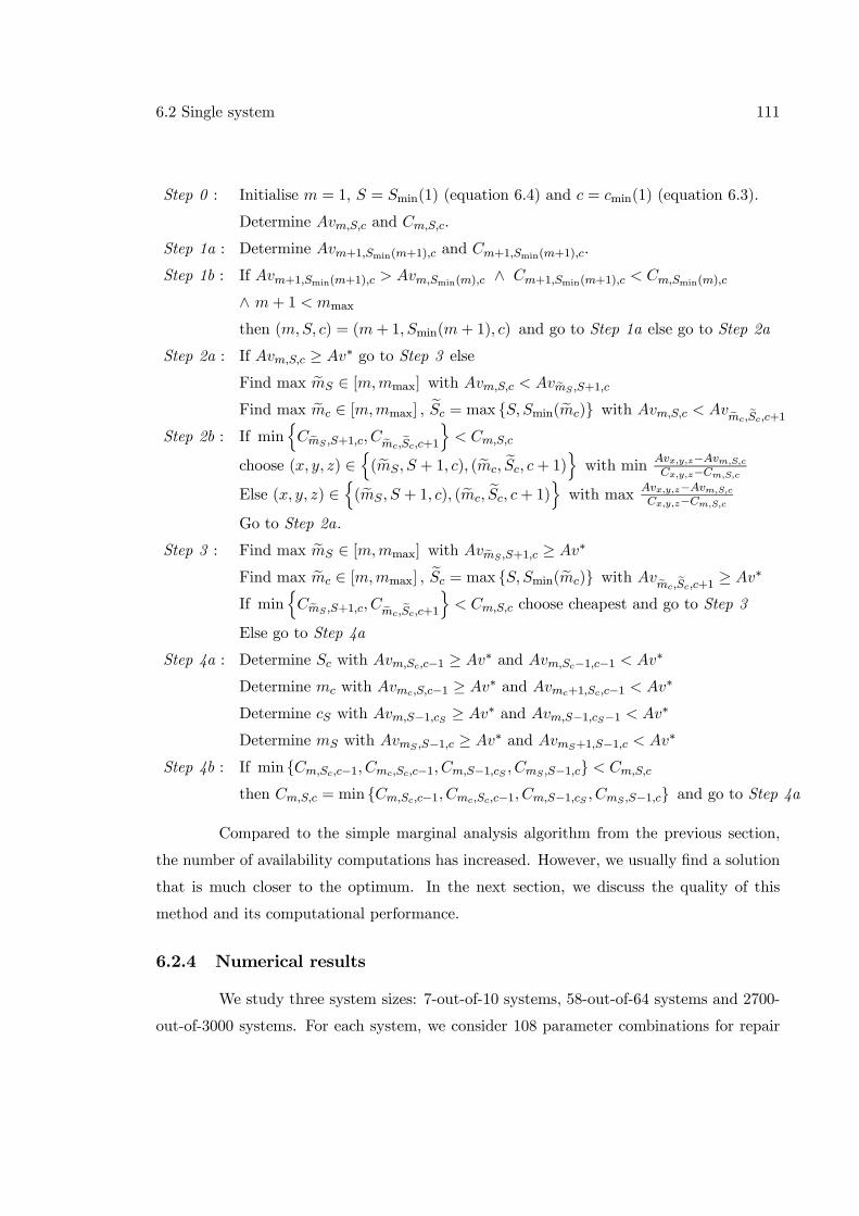
6.2 Single system 111
Step 0 : Initialise m = 1, S = Smin(1) (equation 6.4) and c = cmin(1) (equation 6.3).
Determine Avm,S,c and Cm,S,c.
Step 1a : Determine Avm+1,Smin(m+1),c and Cm+1,Smin(m+1),c.
Step 1b : If Avm+1,Smin(m+1),c > Avm,Smin(m),c ∧ Cm+1,Smin(m+1),c < Cm,Smin(m),c
∧ m+ 1 < mmax
then (m,S, c) = (m+ 1, Smin(m+ 1), c) and go to Step 1a else go to Step 2a
Step 2a : If Avm,S,c ≥ Av∗ go to Step 3 elseFind max emS ∈ [m,mmax] with Avm,S,c < AvemS ,S+1,c
Find max emc ∈ [m,mmax] , eSc = max S, Smin(emc) with Avm,S,c < Avemc,eSc,c+1Step 2b : If min
nCemS ,S+1,c, Cemc,eSc,c+1
o< Cm,S,c
choose (x, y, z) ∈n(emS, S + 1, c), (emc, eSc, c+ 1)o with min Avx,y,z−Avm,S,c
Cx,y,z−Cm,S,c
Else (x, y, z) ∈n(emS , S + 1, c), (emc, eSc, c+ 1)o with max Avx,y,z−Avm,S,c
Cx,y,z−Cm,S,c
Go to Step 2a.
Step 3 : Find max emS ∈ [m,mmax] with AvemS ,S+1,c ≥ Av∗
Find max emc ∈ [m,mmax] , eSc = max S, Smin(emc) with Avemc,eSc,c+1 ≥ Av∗If min
nCemS ,S+1,c, Cemc,eSc,c+1
o< Cm,S,c choose cheapest and go to Step 3
Else go to Step 4a
Step 4a : Determine Sc with Avm,Sc,c−1 ≥ Av∗ and Avm,Sc−1,c−1 < Av∗
Determine mc with Avmc,S,c−1 ≥ Av∗ and Avmc+1,Sc,c−1 < Av∗
Determine cS with Avm,S−1,cS ≥ Av∗ and Avm,S−1,cS−1 < Av∗
Determine mS with AvmS ,S−1,c ≥ Av∗ and AvmS+1,S−1,c < Av∗
Step 4b : If min Cm,Sc,c−1, Cmc,Sc,c−1, Cm,S−1,cS , CmS ,S−1,c < Cm,S,cthen Cm,S,c = min Cm,Sc,c−1, Cmc,Sc,c−1, Cm,S−1,cS , CmS ,S−1,c and go to Step 4a
Compared to the simple marginal analysis algorithm from the previous section,
the number of availability computations has increased. However, we usually find a solution
that is much closer to the optimum. In the next section, we discuss the quality of this
method and its computational performance.
6.2.4 Numerical results
We study three system sizes: 7-out-of-10 systems, 58-out-of-64 systems and 2700-
out-of-3000 systems. For each system, we consider 108 parameter combinations for repair
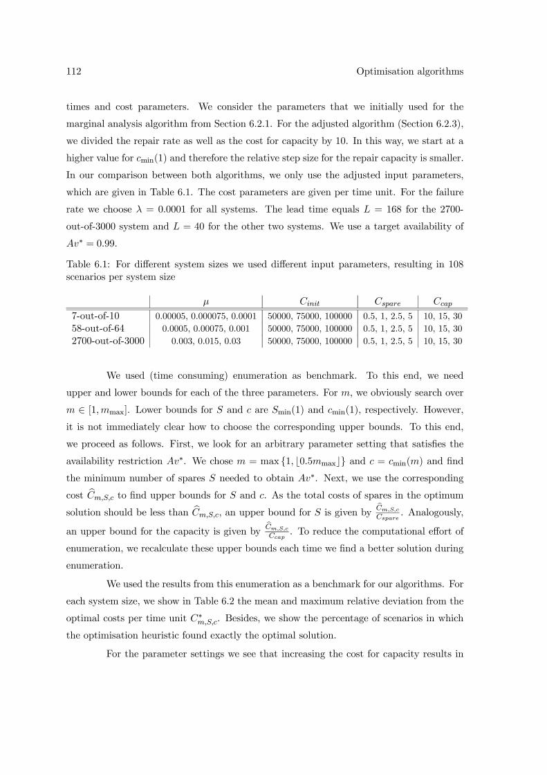
112 Optimisation algorithms
times and cost parameters. We consider the parameters that we initially used for the
marginal analysis algorithm from Section 6.2.1. For the adjusted algorithm (Section 6.2.3),
we divided the repair rate as well as the cost for capacity by 10. In this way, we start at a
higher value for cmin(1) and therefore the relative step size for the repair capacity is smaller.
In our comparison between both algorithms, we only use the adjusted input parameters,
which are given in Table 6.1. The cost parameters are given per time unit. For the failure
rate we choose λ = 0.0001 for all systems. The lead time equals L = 168 for the 2700-
out-of-3000 system and L = 40 for the other two systems. We use a target availability of
Av∗ = 0.99.
Table 6.1: For different system sizes we used different input parameters, resulting in 108scenarios per system size
μ Cinit Cspare Ccap
7-out-of-10 0.00005, 0.000075, 0.0001 50000, 75000, 100000 0.5, 1, 2.5, 5 10, 15, 3058-out-of-64 0.0005, 0.00075, 0.001 50000, 75000, 100000 0.5, 1, 2.5, 5 10, 15, 302700-out-of-3000 0.003, 0.015, 0.03 50000, 75000, 100000 0.5, 1, 2.5, 5 10, 15, 30
We used (time consuming) enumeration as benchmark. To this end, we need
upper and lower bounds for each of the three parameters. For m, we obviously search over
m ∈ [1,mmax]. Lower bounds for S and c are Smin(1) and cmin(1), respectively. However,
it is not immediately clear how to choose the corresponding upper bounds. To this end,
we proceed as follows. First, we look for an arbitrary parameter setting that satisfies the
availability restriction Av∗. We chose m = max 1, b0.5mmaxc and c = cmin(m) and find
the minimum number of spares S needed to obtain Av∗. Next, we use the corresponding
cost bCm,S,c to find upper bounds for S and c. As the total costs of spares in the optimumsolution should be less than bCm,S,c, an upper bound for S is given by bCm,S,c
Cspare. Analogously,
an upper bound for the capacity is given bybCm,S,cCcap
. To reduce the computational effort of
enumeration, we recalculate these upper bounds each time we find a better solution during
enumeration.
We used the results from this enumeration as a benchmark for our algorithms. For
each system size, we show in Table 6.2 the mean and maximum relative deviation from the
optimal costs per time unit C∗m,S,c. Besides, we show the percentage of scenarios in which
the optimisation heuristic found exactly the optimal solution.
For the parameter settings we see that increasing the cost for capacity results in
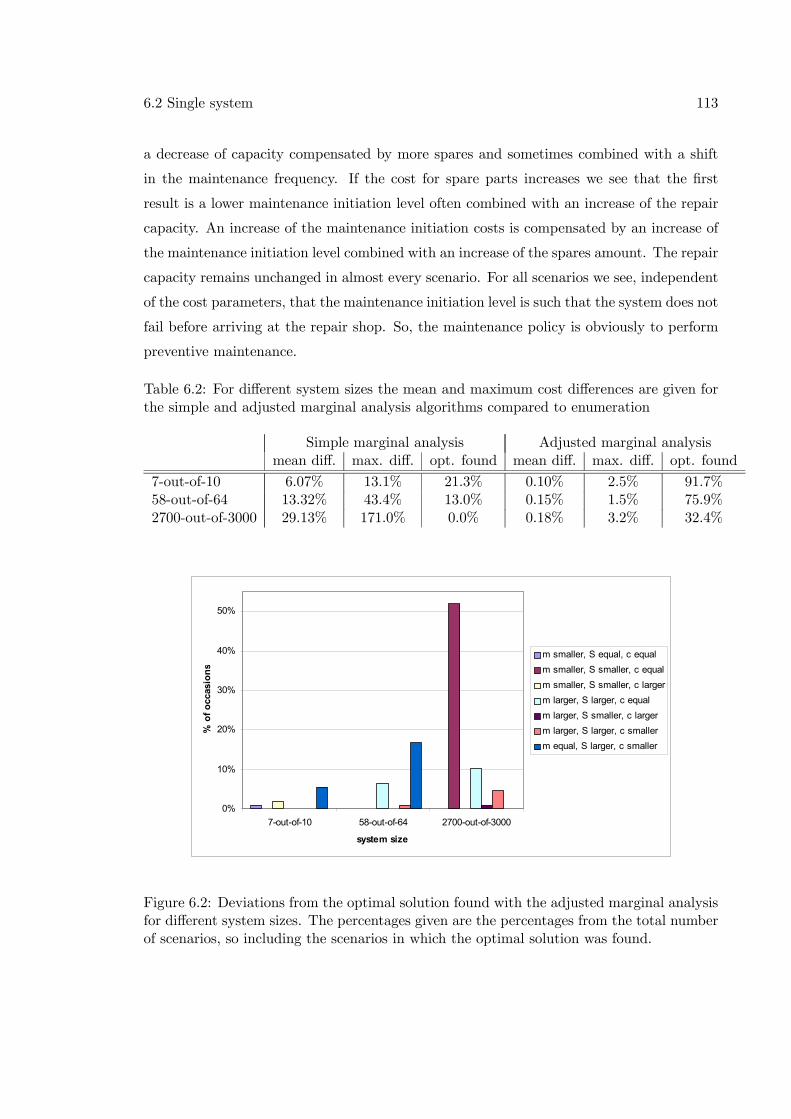
6.2 Single system 113
a decrease of capacity compensated by more spares and sometimes combined with a shift
in the maintenance frequency. If the cost for spare parts increases we see that the first
result is a lower maintenance initiation level often combined with an increase of the repair
capacity. An increase of the maintenance initiation costs is compensated by an increase of
the maintenance initiation level combined with an increase of the spares amount. The repair
capacity remains unchanged in almost every scenario. For all scenarios we see, independent
of the cost parameters, that the maintenance initiation level is such that the system does not
fail before arriving at the repair shop. So, the maintenance policy is obviously to perform
preventive maintenance.
Table 6.2: For different system sizes the mean and maximum cost differences are given forthe simple and adjusted marginal analysis algorithms compared to enumeration
Simple marginal analysis Adjusted marginal analysismean diff. max. diff. opt. found mean diff. max. diff. opt. found
7-out-of-10 6.07% 13.1% 21.3% 0.10% 2.5% 91.7%58-out-of-64 13.32% 43.4% 13.0% 0.15% 1.5% 75.9%2700-out-of-3000 29.13% 171.0% 0.0% 0.18% 3.2% 32.4%
0%
10%
20%
30%
40%
50%
7-out-of-10 58-out-of-64 2700-out-of-3000
system size
% o
f occ
asio
ns
m smaller, S equal, c equalm smaller, S smaller, c equalm smaller, S smaller, c largerm larger, S larger, c equalm larger, S smaller, c largerm larger, S larger, c smallerm equal, S larger, c smaller
Figure 6.2: Deviations from the optimal solution found with the adjusted marginal analysisfor different system sizes. The percentages given are the percentages from the total numberof scenarios, so including the scenarios in which the optimal solution was found.
114 Optimisation algorithms
We see that the enhanced marginal analysis algorithm yields much better solutions
than the straightforward marginal approach. Using our enhanced algorithm we also find the
exact optimum solution more frequently. For the cases in which the parameter setting of
the adjusted marginal analysis differs from the optimal solution, we can classify the type of
deviation, see Figure 6.2. It shows the percentage of each type of deviation as a percentage
of the total number of scenarios. We see that for the large systems we find too small values
for m and S in most cases. For smaller systems, we tend to find the optimal value of m
combined with too large values for S and too small values for c.
The deviations that are relatively large, more than one percent, are mainly caused
by too many spares and too few capacity. In these cases we end up in a local minimum from
which we do not reach the global minimum by balancing the spares and capacity using our
heuristic. In Figure 6.3 we illustrate the balancing step of the algorithm. The parameter
setting marked as 0 is the solution we find after the third step. From there we have the
possibilities to improve the costs by moving to one of the black dots. Obviously, the option
marked as 1 is the cheapest. Finally, we end up in the red dot instead of the green one.
Unless we would except more expensive solutions, we are not able to make the change to
the line with m = 3, c = 12.
When we consider the utilisation rates, the differences are small as can be seen
from Table 6.3. The deviating utilisation rates are always found in the scenarios where the
parameter setting of the adjusted marginal analysis has a too large number of spares and a
too small number of capacity (sometimes combined with a maintenance initiation level that
is too large). So, we may conclude from this table that the utilisation rate is not affected
very much if we do not find the optimal parameter setting in all cases.
Table 6.3: For different system sizes the average utilisation rates are given for the solutionsfound using enumeration and the adjusted marginal analysis
enumeration adjusted marg. analysismin. mean max. min. mean max.
7-out-of-10 73.5% 81.4% 83.3% 78.4% 81.8% 89.0%58-out-of-64 61.0% 85.3% 93.8% 74.0% 86.9% 93.8%2700-out-of-3000 81.5% 92.4% 97.6% 81.5% 92.8% 98.0%
In Table 6.4 we show the average number of availability computations per solution
method. We see that the additional computational effort for the optimisation algorithm
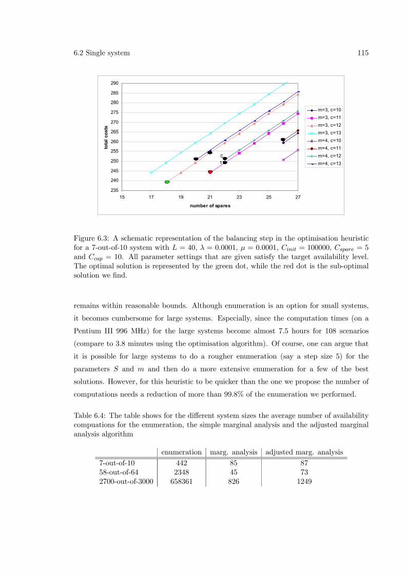
6.2 Single system 115
235
240
245
250
255
260
265
270
275
280
285
290
15 17 19 21 23 25 27
number of spares
tota
l cos
tsm=3, c=10m=3, c=11m=3, c=12m=3, c=13m=4, c=10m=4, c=11m=4, c=12m=4, c=13
01
Figure 6.3: A schematic representation of the balancing step in the optimisation heuristicfor a 7-out-of-10 system with L = 40, λ = 0.0001, μ = 0.0001, Cinit = 100000, Cspare = 5and Ccap = 10. All parameter settings that are given satisfy the target availability level.The optimal solution is represented by the green dot, while the red dot is the sub-optimalsolution we find.
remains within reasonable bounds. Although enumeration is an option for small systems,
it becomes cumbersome for large systems. Especially, since the computation times (on a
Pentium III 996 MHz) for the large systems become almost 7.5 hours for 108 scenarios
(compare to 3.8 minutes using the optimisation algorithm). Of course, one can argue that
it is possible for large systems to do a rougher enumeration (say a step size 5) for the
parameters S and m and then do a more extensive enumeration for a few of the best
solutions. However, for this heuristic to be quicker than the one we propose the number of
computations needs a reduction of more than 99.8% of the enumeration we performed.
Table 6.4: The table shows for the different system sizes the average number of availabilitycompuations for the enumeration, the simple marginal analysis and the adjusted marginalanalysis algorithm
enumeration marg. analysis adjusted marg. analysis
7-out-of-10 442 85 8758-out-of-64 2348 45 732700-out-of-3000 658361 826 1249
116 Optimisation algorithms
There is however one disadvantage when using this optimisation algorithm. The
algorithm finds a near-optimal solution, but not via a path of near-optimal solutions for
various target availability levels as is true for METRIC. This property of METRIC can be
used to construct an availability-cost trade-off curve. As a consequence, in principle we have
to start our computations all over again if the target availability level changes. Of course,
one could use the solution found for a certain target availability as initial value to find the
best solution for a somewhat higher target availability, just like METRIC. However, some
experiments revealed that this may lead to inferior results.
6.2.5 Extension to component wear-out
Until now, we only considered the model in which all components have an exponen-
tially distributed time to failure. In this section we show how our approach can be extended
to include wear-out (Chapter 3). The only adjustments needed are the initial values cmin(1)
and Smin(m). We need the expected number of components in state 1 and state 2. We
know these expectations from equations 3.30 and 3.32 and E [A1] = N − E [A0] − E [A2].Obviously, the values for E [A1] and E [A2] are functions of the parameter m. As a result
we find for the lower bound of spares:
Smin(m) = bE [A1(m)] +E [A2(m)]c (6.5)
For the lower bound of the capacity we use a weighted average for the repair rate,
which is also a function of the parameter m:
μ(m) =E [A1(m)]
E [A1(m)] +E [A2(m)]μ1 +
E [A2(m)]
E [A1(m)] +E [A2(m)]μ2 (6.6)
Combining the expected system state at arrival in the repair shop with the weighted
average repair rate and the target availability, we find:
cmin(m) =
»E [A1(m)] +E [A2(m)]
(E [Tm] + L)μ(m)Av∗
¼(6.7)
6.3 Multiple systems
In this section, we consider optimisation of the model for an installed base of
systems as discussed in Chapters 4 and 5. We show that we can modify our adjusted
6.3 Multiple systems 117
marginal analysis algorithm rather easily to deal with an installed base of systems. We
start with the model without wear out. Afterwards, we discuss how component wear-out
can be included in the model.
We define our optimisation problem as follows:
minCinitT
+ SCspare + cCcapacity
s.t. AvT,S,c ≥ Av∗
where T denotes the fixed maintenance interval and the other notation is identical
to the previous section. The decision variables are T , S and c. The optimisation problem is
basically the same as the one discussed in the previous section, with the key difference that
we now have a continuous maintenance parameter T instead of the discrete maintenance
initiation level m. Therefore we can expect to encounter the same issues as in Section
6.2.2, including the non-monotonous relation between the availability and the maintenance
frequency. Although we do not have a lead time now, the availability still decreases if the
maintenance interval becomes too small. This is due to the fact that during the very short
time between maintenance instances the repair shop is not able to restore spare parts and
therefore the fraction of T that is needed for maintenance increases. Another reason is the
fact that the speed at which components fail decreases as T increases. Components can fail
only once and the number of components subject to failure decreases over time.
6.3.1 Adjusted marginal analysis algorithm
The main modification needed to apply our algorithm from Section 6.2.3 to the
installed base model is to replace the discrete parameter m for maintenance initiation by
the continuous parameter T for the fixed time between preventive maintenance epochs of
a single system in the installed base. Just like in the situation of a single system we can
determine a minimum value for the interval length Tmin (analogous to m = 1 for the single
system) as well as a maximum value Tmax for T (analogous to m = mmax for the single
system). To find these boundaries for T , we discretise the interval length by choosing
the values of T such that they correspond with an integer number m of expected failures
before the start of maintenance. The expected time until the first component failure equals1Nλ . Including the maximum maintenance duration for which the system availability is
118 Optimisation algorithms
at least equal to Av∗ we find Tmin = 1NλAv∗ as a lower bound for the total time between
succeeding maintenance instances. Analogously, we findm−1Pi=0
1(N−i)λ for the maintenance
interval corresponding to m expected failures at system arrival at the repair shop. This also
gives us an upper bound for the interval length, which is found in the maintenance interval
corresponding to N − k + 1 failures. Hence, we find 1Av∗
N−kPi=0
1(N−i)λ . If T would be larger
than this value we would introduce extra down time only (no additional operational time is
acquired since the number of failed components already exceeds N − k) and as a result thesystem availability drops below the required Av∗, even if the maintenance duration would
be zero.
Just like the case of a single system it may happen that with this value of T =
1Av∗
N−kPi=0
1(N−i)λ it is impossible to achieve the desired availability Av
∗, even if there are no
bottlenecks caused by the number of spares or repair capacity. Therefore, we search for the
largest number of failures, mmax, such that we cannot achieve Av∗ while we can achieve
Av∗ if the number of failures is decreased by one. Hence, we find the interval containing
Tmax:
Tmax ∈"1
Av∗
mmax−2Xi=0
1
(N − i)λ ,1
Av∗
mmax−1Xi=0
1
(N − i)λ
#with 1 ≤ mmax ≤ N − k + 1 (6.9)
The left boundary of this interval in which Tmax lies is such that the maximum
availability is larger than Av∗ and in the right boundary the maximum availability is lower
than Av∗. Using a standard bi-section method, we find the value of Tmax.
In this section we discuss our modifications to the algorithm of Section 6.2.3 to
deal with the installed base model. Just like the in the previous section we concentrate on
the case in which the components are not subject to wear-out.
Step 0: initialisation
Analogously to the previous algorithm we start with the determination of the
initial values for the decision variables T , S and c. Again we start with a small maintenance
interval. Just like we chose m = 1 in the Section 6.2.3, we choose the maintenance interval
corresponding to the expected time until a single component failure as initial value for T ,
so Tmin = 1NλAv∗ .
6.3 Multiple systems 119
For the minimum repair capacity we choose the interval length corresponding to
the initial value of T (analogously to the situation with m = 1 in the single system case,
see Section 6.2.3), so Tmin = 1NλAv∗ . This results in a minimum capacity of:
cmin =
&MN
¡1− e−λTminAv∗
¢μTmin
'=
⎡⎢⎢⎢MN2λAv∗
³1− e− 1
N
´μ
⎤⎥⎥⎥For the minimum number of spares we use the equivalent of m for a continuous
parameter T :
Smin(Tmin) =jMN
³1− e−λTminAv∗
´kThe initial value for the number of spares equals Smin
¡1
NλAv∗¢.
Step 1: improving availability without increasing costs
In this step we increase the maintenance interval until there is no further incre-
ment possible without either increasing the costs per time unit or reducing the availability.
We start by increasing the parameter T discretely such that each increment corresponds
to increasing the expected number of failures at arrival for maintenance by one (equivalent
to increasing m by one, in case of the single system). Therefore, the values of T become
1Av∗
1Pi=0
1(N−i)λ ,
1Av∗
2Pi=0
1(N−i)λ ,...,Tmax. Tmax is the maximum length of the maintenance inter-
val for which it is possible to obtain the required availability level Av∗ as explained earlier
in this section (see equation 6.9).
As long as there is a cost reduction and the availability increases, we increase the
interval T discretely (under the condition that T ≤ Tmax). Together with the increasingmaintenance interval we increase the number of spares if the number of spares becomes
less than Smin(T ). If there is no increment of the maintenance interval possible anymore
(and T < Tmax) we use the bi-section method to find a more precise value of T . So,
suppose we found T = 1Av∗
2Pi=0
1(N−i)λ and for T = 1
Av∗
3Pi=0
1(N−i)λ either the costs increase
or the availability decreases. Then we search for the largest possible value for T , with
T ∈∙
1Av∗
2Pi=0
1(N−i)λ ,
1Av∗
3Pi=0
1(N−i)λ
¸that improves the availability without increasing the
costs using bi-section.
120 Optimisation algorithms
Step 2: improving availability until Av∗ with acceptance of increasing costs
For the second step in the algorithm we either increase the capacity or the number
of spares together with an increase of T as much as possible without a reduction of the
availability. If increasing the capacity and T implies that the expected number of failed
components at arrival in the repair shop increases (S < Smin(T )), we also increase the spare
part level S. So, we do basically the same with parameter T as we did in the previous step.
We start with the value for T we found in step 1 and increase T to the largest discrete point
we mentioned in the previous step resulting in an increase of the availability. Knowing that
the maintenance interval length we are looking for lies between this value of T and the next
higher discrete point we again use bi-section to find the right interval length.
Step 3: reducing costs by increasing T and maintaining Av∗
The third step of the algorithm is, just like in the algorithm for the single system,
the same as step 2 except for the fact that we only accept cost reductions.
Step 4: balancing the parameter setting
In the fourth step we have two options that do not involve adjusting the mainte-
nance interval length. Therefore, these options remain unchanged. The other two options
do need adjustments because the maintenance interval length is decreased. The idea is to
use a bi-section again with the right boundary TR equal to the interval length we found
thus far. The left boundary TL is found as follows. The decrease of the spares or capac-
ity (dependent on the considered option) gives an increase of the system down time. The
relative increase of the down time is the same ratio we use to decrease TR to TL. This TL
is an underestimation for the maintenance interval length due to the fact that we adjust
the maintenance interval only based on the increase of the maintenance duration resulting
from the capacity reduction. Decreasing the maintenance interval also has an impact on the
operational time until maintenance is performed. We can now determine T by searching
the interval [TL, TR] using bi-section. However, to find the value of T more quickly, we
use linear interpolation between TL and TR first, finding a value T ∗. If T ∗ results in an
availability level larger than Av∗, we find T ∈ [T ∗, TR]. Otherwise, we have T ∈ [TL, T ∗].Now, we perform a bi-section again to find the maintenance interval length T .
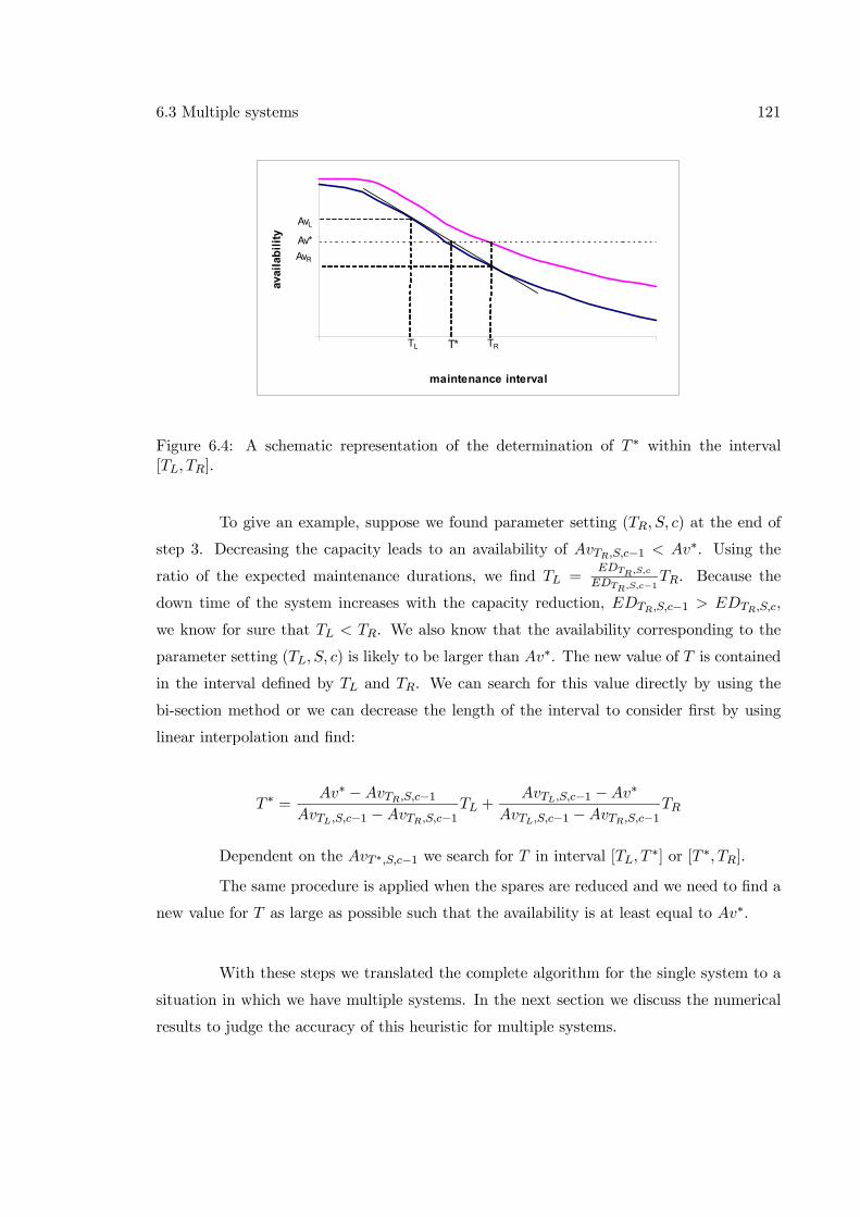
6.3 Multiple systems 121
0.95
1
500 1500
maintenance interval
avai
labi
lity
TL TR
AvL
AvR
T*
Av*
Figure 6.4: A schematic representation of the determination of T ∗ within the interval[TL, TR].
To give an example, suppose we found parameter setting (TR, S, c) at the end of
step 3. Decreasing the capacity leads to an availability of AvTR,S,c−1 < Av∗. Using the
ratio of the expected maintenance durations, we find TL =EDTR,S,cEDTR,S,c−1
TR. Because the
down time of the system increases with the capacity reduction, EDTR,S,c−1 > EDTR,S,c,
we know for sure that TL < TR. We also know that the availability corresponding to the
parameter setting (TL, S, c) is likely to be larger than Av∗. The new value of T is contained
in the interval defined by TL and TR. We can search for this value directly by using the
bi-section method or we can decrease the length of the interval to consider first by using
linear interpolation and find:
T ∗ =Av∗ −AvTR,S,c−1
AvTL,S,c−1 −AvTR,S,c−1TL +
AvTL,S,c−1 −Av∗AvTL,S,c−1 −AvTR,S,c−1
TR
Dependent on the AvT∗,S,c−1 we search for T in interval [TL, T ∗] or [T ∗, TR].
The same procedure is applied when the spares are reduced and we need to find a
new value for T as large as possible such that the availability is at least equal to Av∗.
With these steps we translated the complete algorithm for the single system to a
situation in which we have multiple systems. In the next section we discuss the numerical
results to judge the accuracy of this heuristic for multiple systems.
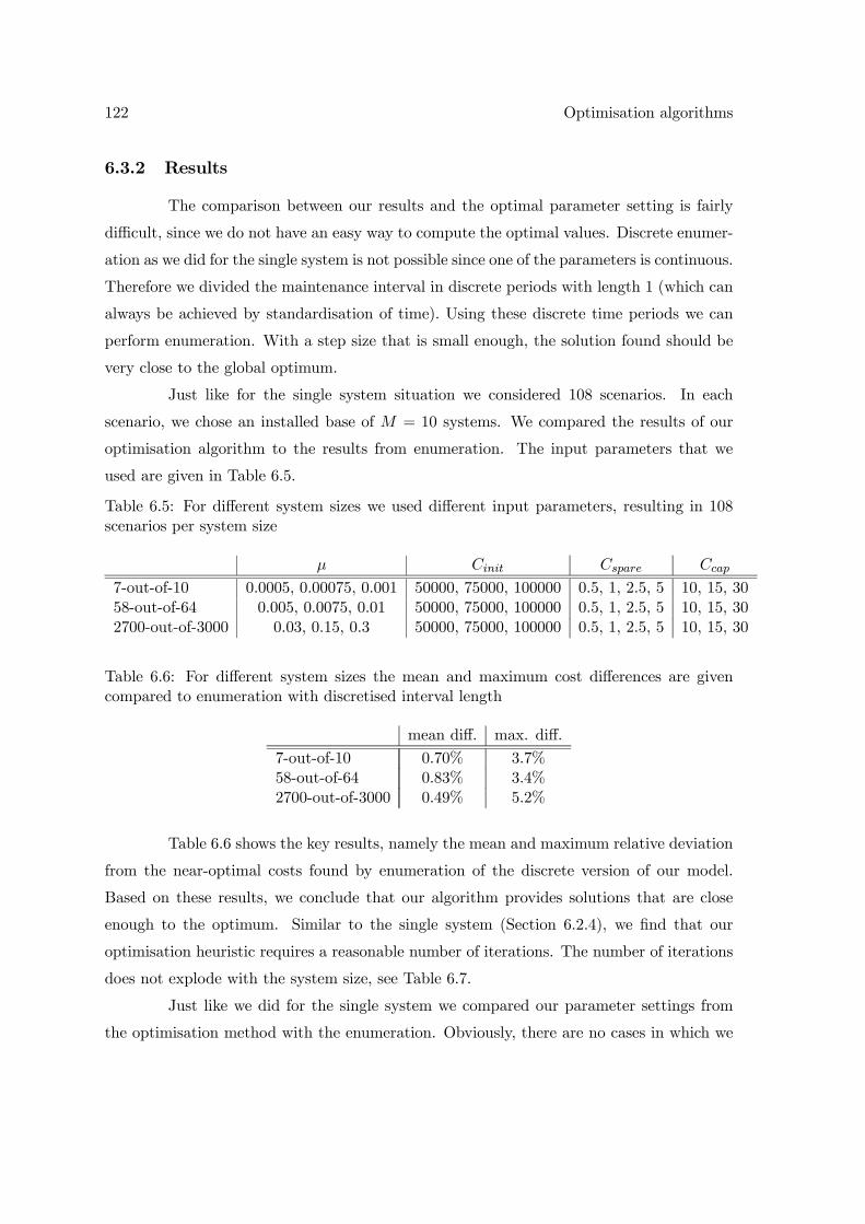
122 Optimisation algorithms
6.3.2 Results
The comparison between our results and the optimal parameter setting is fairly
difficult, since we do not have an easy way to compute the optimal values. Discrete enumer-
ation as we did for the single system is not possible since one of the parameters is continuous.
Therefore we divided the maintenance interval in discrete periods with length 1 (which can
always be achieved by standardisation of time). Using these discrete time periods we can
perform enumeration. With a step size that is small enough, the solution found should be
very close to the global optimum.
Just like for the single system situation we considered 108 scenarios. In each
scenario, we chose an installed base of M = 10 systems. We compared the results of our
optimisation algorithm to the results from enumeration. The input parameters that we
used are given in Table 6.5.
Table 6.5: For different system sizes we used different input parameters, resulting in 108scenarios per system size
μ Cinit Cspare Ccap
7-out-of-10 0.0005, 0.00075, 0.001 50000, 75000, 100000 0.5, 1, 2.5, 5 10, 15, 3058-out-of-64 0.005, 0.0075, 0.01 50000, 75000, 100000 0.5, 1, 2.5, 5 10, 15, 302700-out-of-3000 0.03, 0.15, 0.3 50000, 75000, 100000 0.5, 1, 2.5, 5 10, 15, 30
Table 6.6: For different system sizes the mean and maximum cost differences are givencompared to enumeration with discretised interval length
mean diff. max. diff.
7-out-of-10 0.70% 3.7%58-out-of-64 0.83% 3.4%2700-out-of-3000 0.49% 5.2%
Table 6.6 shows the key results, namely the mean and maximum relative deviation
from the near-optimal costs found by enumeration of the discrete version of our model.
Based on these results, we conclude that our algorithm provides solutions that are close
enough to the optimum. Similar to the single system (Section 6.2.4), we find that our
optimisation heuristic requires a reasonable number of iterations. The number of iterations
does not explode with the system size, see Table 6.7.
Just like we did for the single system we compared our parameter settings from
the optimisation method with the enumeration. Obviously, there are no cases in which we
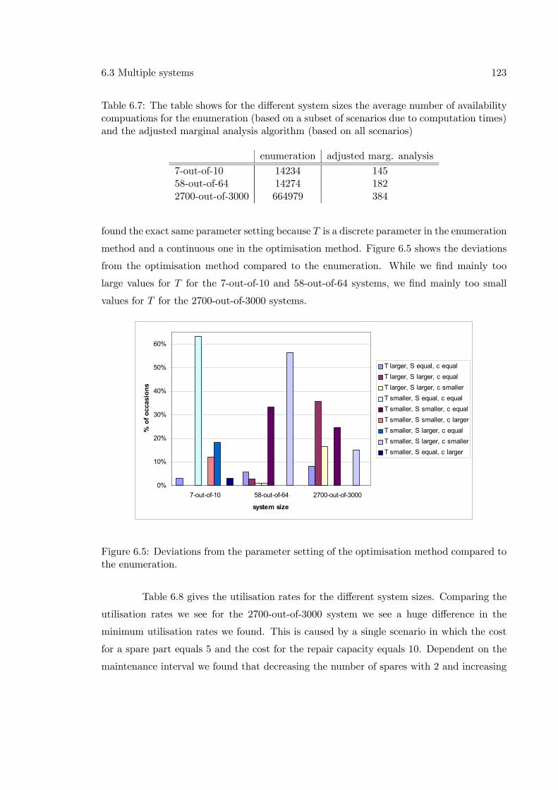
6.3 Multiple systems 123
Table 6.7: The table shows for the different system sizes the average number of availabilitycompuations for the enumeration (based on a subset of scenarios due to computation times)and the adjusted marginal analysis algorithm (based on all scenarios)
enumeration adjusted marg. analysis
7-out-of-10 14234 14558-out-of-64 14274 1822700-out-of-3000 664979 384
found the exact same parameter setting because T is a discrete parameter in the enumeration
method and a continuous one in the optimisation method. Figure 6.5 shows the deviations
from the optimisation method compared to the enumeration. While we find mainly too
large values for T for the 7-out-of-10 and 58-out-of-64 systems, we find mainly too small
values for T for the 2700-out-of-3000 systems.
0%
10%
20%
30%
40%
50%
60%
7-out-of-10 58-out-of-64 2700-out-of-3000
system size
% o
f occ
asio
ns
T larger, S equal, c equalT larger, S larger, c equalT larger, S larger, c smallerT smaller, S equal, c equalT smaller, S smaller, c equalT smaller, S smaller, c largerT smaller, S larger, c equalT smaller, S larger, c smallerT smaller, S equal, c larger
Figure 6.5: Deviations from the parameter setting of the optimisation method compared tothe enumeration.
Table 6.8 gives the utilisation rates for the different system sizes. Comparing the
utilisation rates we see for the 2700-out-of-3000 system we see a huge difference in the
minimum utilisation rates we found. This is caused by a single scenario in which the cost
for a spare part equals 5 and the cost for the repair capacity equals 10. Dependent on the
maintenance interval we found that decreasing the number of spares with 2 and increasing
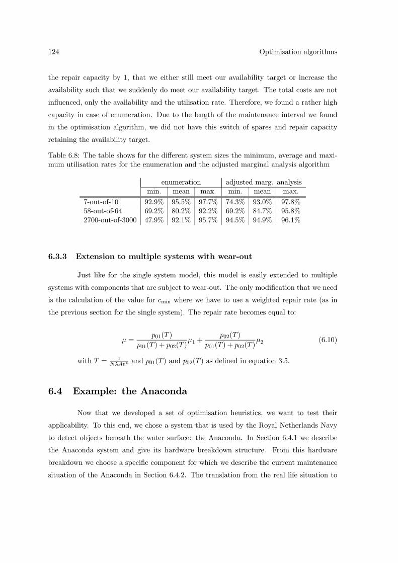
124 Optimisation algorithms
the repair capacity by 1, that we either still meet our availability target or increase the
availability such that we suddenly do meet our availability target. The total costs are not
influenced, only the availability and the utilisation rate. Therefore, we found a rather high
capacity in case of enumeration. Due to the length of the maintenance interval we found
in the optimisation algorithm, we did not have this switch of spares and repair capacity
retaining the availability target.
Table 6.8: The table shows for the different system sizes the minimum, average and maxi-mum utilisation rates for the enumeration and the adjusted marginal analysis algorithm
enumeration adjusted marg. analysismin. mean max. min. mean max.
7-out-of-10 92.9% 95.5% 97.7% 74.3% 93.0% 97.8%58-out-of-64 69.2% 80.2% 92.2% 69.2% 84.7% 95.8%2700-out-of-3000 47.9% 92.1% 95.7% 94.5% 94.9% 96.1%
6.3.3 Extension to multiple systems with wear-out
Just like for the single system model, this model is easily extended to multiple
systems with components that are subject to wear-out. The only modification that we need
is the calculation of the value for cmin where we have to use a weighted repair rate (as in
the previous section for the single system). The repair rate becomes equal to:
μ =p01(T )
p01(T ) + p02(T )μ1 +
p02(T )
p01(T ) + p02(T )μ2 (6.10)
with T = 1NλAv∗ and p01(T ) and p02(T ) as defined in equation 3.5.
6.4 Example: the Anaconda
Now that we developed a set of optimisation heuristics, we want to test their
applicability. To this end, we chose a system that is used by the Royal Netherlands Navy
to detect objects beneath the water surface: the Anaconda. In Section 6.4.1 we describe
the Anaconda system and give its hardware breakdown structure. From this hardware
breakdown we choose a specific component for which we describe the current maintenance
situation of the Anaconda in Section 6.4.2. The translation from the real life situation to
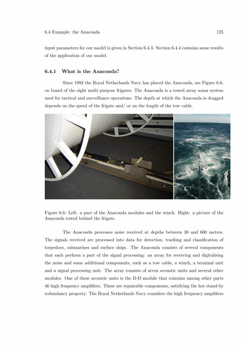
6.4 Example: the Anaconda 125
input parameters for our model is given in Section 6.4.3. Section 6.4.4 contains some results
of the application of our model.
6.4.1 What is the Anaconda?
Since 1992 the Royal Netherlands Navy has placed the Anaconda, see Figure 6.6,
on board of the eight multi purpose frigates. The Anaconda is a towed array sonar system
used for tactical and surveillance operations. The depth at which the Anaconda is dragged
depends on the speed of the frigate and/ or on the length of the tow cable.
Figure 6.6: Left: a part of the Anaconda modules and the winch. Right: a picture of theAnaconda towed behind the frigate.
The Anaconda processes noise received at depths between 30 and 600 metres.
The signals received are processed into data for detection, tracking and classification of
torpedoes, submarines and surface ships. The Anaconda consists of several components
that each perform a part of the signal processing: an array for receiving and digitalising
the noise and some additional components, such as a tow cable, a winch, a terminal unit
and a signal processing unit. The array consists of seven acoustic units and several other
modules. One of these acoustic units is the D-D module that contains among other parts
46 high frequency amplifiers. These are repairable components, satisfying the hot stand-by
redundancy property. The Royal Netherlands Navy considers the high frequency amplifiers
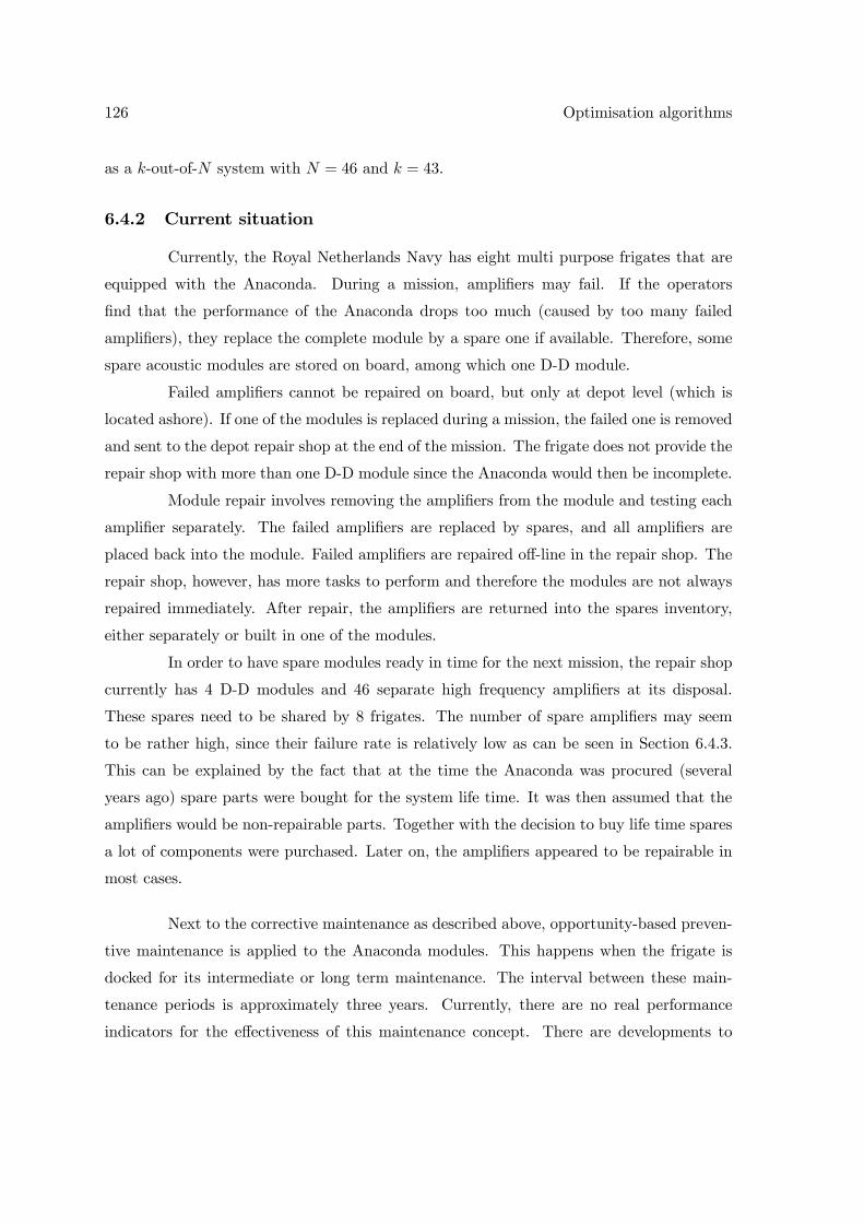
126 Optimisation algorithms
as a k-out-of-N system with N = 46 and k = 43.
6.4.2 Current situation
Currently, the Royal Netherlands Navy has eight multi purpose frigates that are
equipped with the Anaconda. During a mission, amplifiers may fail. If the operators
find that the performance of the Anaconda drops too much (caused by too many failed
amplifiers), they replace the complete module by a spare one if available. Therefore, some
spare acoustic modules are stored on board, among which one D-D module.
Failed amplifiers cannot be repaired on board, but only at depot level (which is
located ashore). If one of the modules is replaced during a mission, the failed one is removed
and sent to the depot repair shop at the end of the mission. The frigate does not provide the
repair shop with more than one D-D module since the Anaconda would then be incomplete.
Module repair involves removing the amplifiers from the module and testing each
amplifier separately. The failed amplifiers are replaced by spares, and all amplifiers are
placed back into the module. Failed amplifiers are repaired off-line in the repair shop. The
repair shop, however, has more tasks to perform and therefore the modules are not always
repaired immediately. After repair, the amplifiers are returned into the spares inventory,
either separately or built in one of the modules.
In order to have spare modules ready in time for the next mission, the repair shop
currently has 4 D-D modules and 46 separate high frequency amplifiers at its disposal.
These spares need to be shared by 8 frigates. The number of spare amplifiers may seem
to be rather high, since their failure rate is relatively low as can be seen in Section 6.4.3.
This can be explained by the fact that at the time the Anaconda was procured (several
years ago) spare parts were bought for the system life time. It was then assumed that the
amplifiers would be non-repairable parts. Together with the decision to buy life time spares
a lot of components were purchased. Later on, the amplifiers appeared to be repairable in
most cases.
Next to the corrective maintenance as described above, opportunity-based preven-
tive maintenance is applied to the Anaconda modules. This happens when the frigate is
docked for its intermediate or long term maintenance. The interval between these main-
tenance periods is approximately three years. Currently, there are no real performance
indicators for the effectiveness of this maintenance concept. There are developments to
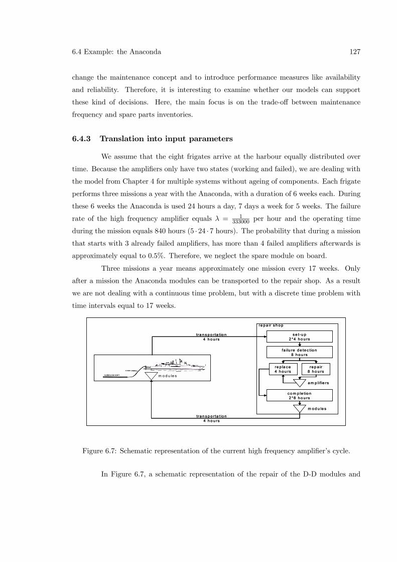
6.4 Example: the Anaconda 127
change the maintenance concept and to introduce performance measures like availability
and reliability. Therefore, it is interesting to examine whether our models can support
these kind of decisions. Here, the main focus is on the trade-off between maintenance
frequency and spare parts inventories.
6.4.3 Translation into input parameters
We assume that the eight frigates arrive at the harbour equally distributed over
time. Because the amplifiers only have two states (working and failed), we are dealing with
the model from Chapter 4 for multiple systems without ageing of components. Each frigate
performs three missions a year with the Anaconda, with a duration of 6 weeks each. During
these 6 weeks the Anaconda is used 24 hours a day, 7 days a week for 5 weeks. The failure
rate of the high frequency amplifier equals λ = 1333000 per hour and the operating time
during the mission equals 840 hours (5 ·24 · 7 hours). The probability that during a missionthat starts with 3 already failed amplifiers, has more than 4 failed amplifiers afterwards is
approximately equal to 0.5%. Therefore, we neglect the spare module on board.
Three missions a year means approximately one mission every 17 weeks. Only
after a mission the Anaconda modules can be transported to the repair shop. As a result
we are not dealing with a continuous time problem, but with a discrete time problem with
time intervals equal to 17 weeks.
m o d u le s
s e t-u p2 *4 h o u rs
re p la c e4 h o u rs
re p a ir8 h o u rs
fa ilu re d e te c t io n8 h o u rs
c o m p le t io n2 *8 h o u rs
m o d u le s
a m p lif ie rs
re p a ir s h o p
tra n s p o r ta t io n4 h o u rs
tra n s p o r ta t io n4 h o u rs
m o d u le s
s e t-u p2 *4 h o u rs
re p la c e4 h o u rs
re p a ir8 h o u rs
fa ilu re d e te c t io n8 h o u rs
c o m p le t io n2 *8 h o u rs
m o d u le s
a m p lif ie rs
re p a ir s h o p
tra n s p o r ta t io n4 h o u rs
tra n s p o r ta t io n4 h o u rs
Figure 6.7: Schematic representation of the current high frequency amplifier’s cycle.
In Figure 6.7, a schematic representation of the repair of the D-D modules and
128 Optimisation algorithms
the high frequency amplifiers of the Anaconda is depicted. Both the set-up and completion
need to be done by two persons. This means that the calendar time needed is respectively
4 and 8 hours and the costs involved are respectively 8 and 16 times the hourly wages.
The transportation requires time that cannot be influenced by the repair capacity. So, it
is not really part of the maintenance activities and it is not a lead time either because the
system is not in use. We have similar situations with the set-up time in the repair shop,
the replacement time and the completion time. We choose to subtract these time durations
from the first 17 weeks mission duration, as it is down time that can only be influenced by
the maintenance frequency. The duration of all repair related activities equals:
• 4 hours transportation time from the frigate to the repair shop,
• 4 hours set-up time in the repair shop,
• 8 hours for failure detection per module,
• 4 hours for the replacement time per failed component,
• 8 hours completion time,
• 4 hours transportation time from the repair shop to the frigate.
We assume the maintenance intervals in a cost optimal situation to be a multiple
of the mission length. Therefore we assume that the total replacement time equals 16 hours,
corresponding to 4 failed components. If the number of failed components is likely to be
larger than 4, we are dealing with a maintenance frequency that is obviously too low to
obtain high availability levels. As a consequence, the down time is 44 hours. As a standard
working week contains 40 hours instead of 168 we have to multiply the down time by 4.2 to
translate it to calendar time, resulting in 184.8 hours. For the repair time we know that it
takes 8 working hours, which is 33.6 hours in calendar time. So, μ = 133.6 .
Summarised, we use the following input parameters:
6.4 Example: the Anaconda 129
M = 8 frigates
k = 43 amplifiers
N = 46 amplifiers
T = 2856i− 184.8 hours
λ =1
333000
840
2856= 8.8 · 10−7 per hour
μ =1
33.6per hour
We introduce i to indicate the number of missions between successive arrivals for
maintenance. In the current situation we have c = 1 and maintenance after each mission.
This implies i = 1 and T = 2671.2. The number of spare amplifiers is 4 · 46 as part of the 4spare modules ashore plus 46 separate amplifiers, which equals 230 spares (230+8 ·46 = 598if we include the spare modules on board the frigates).
The hourly cost for transportation is 20, 72 Euro and the hourly cost of personnel
at the repair shop is 24, 26 Euro per hour. So, the initial costs for maintenance set-up
consist of:
• 2 times (back and forth) 4 hours transportation costing 165.76 Euros in total,
• 4 hours set-up time with 2 persons costing 194.08 Euros,
• 16 hours for replacements costing 388.16 Euros,
• 8 hours for completion with 2 persons costing 388.16 Euros.
The total set-up costs are 1136 Euros. The costs for a single spare part are 3700
Euros, assuming the life time of a spare to be 20 years we find 0.022 Euros per hour
( 370020·3·17·168).
The maintenance time is very small compared to the operational times, therefore
we need to adjust the capacity. To avoid the problem mentioned in Section 6.2.2 as issue
1, we define the capacity step size such that we need at least 10 units of capacity. Hence,
cmin = 10 and the utilisation rate of the repair shop does not fall from very high to very low
when one unit of capacity is added. Due to the small maintenance times compared to the
130 Optimisation algorithms
operational times we need small capacity units. We have chosen the capacity equivalent to
10 minutes per week or 0.004 fte. We adjust the repair rate and the costs accordingly and
find μ = 2.95 · 10−5 and Ccap = 0.024 Euro.In this case, we set the value of T to be a multiple of the mission duration. So if
the maintenance frequency is once per 3 missions (once a year) we use T = 2856∗3−184.8.We therefore do not need the extra steps in the algorithm with the bi-section method, we
only need the discrete points in time at the end of a mission.
The operational availability also needs to be adjusted a little due to the 184.8
hours of down time that cannot be influenced. We adjust the availability calculation in the
model to:
Av =E [U (T −D)]T + 184.8
Because we only consider the options of maintenance between missions, we only
have to consider a limited number of values for T . This simplifies our algorithm. However,
because we discrete values for T and we have a number of downtime hours that cannot be
influenced, we are not able to achieve an availability level of 100%. The highest possible
availability we can achieve is almost 98.9% (considering the largest possible interval, the
expected time until the fourth amplifier fails, and the maintenance duration equals zero).
6.4.4 Results
Using the input parameters given in the previous section, we find the results for
different target levels for the availability, given in Table 6.9. As can be seen, the parameter
setting found for the target availability of 0.9 is not the optimal one since the parameter
setting with Av∗ = 0.925 has lower costs. However, the cost difference is small, only
1.3%. Furthermore, we see that the cost increment becomes larger as the target availability
increases, as could be expected.
With a maintenance period every 6 years (corresponding to 18 missions), a module
contains two failed amplifiers on average upon arrival at the repair shop. The probability
of having a failed module (more than three failed amplifiers) after the operational time of
6 years is 0.14. So, maintenance is mostly performed before a failure of the module occurs.
Taking into account a spare module on board, the probability of having a disfunctioning
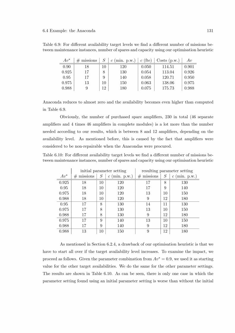
6.4 Example: the Anaconda 131
Table 6.9: For different availability target levels we find a different number of missions be-tween maintenance instances, number of spares and capacity using our optimisation heuristic
Av∗ # missions S c (min. p.w.) c (fte) Costs (p.w.) Av
0.90 18 10 120 0.050 114.51 0.9010.925 17 8 130 0.054 113.04 0.9260.95 17 9 140 0.058 120.71 0.9500.975 13 10 150 0.063 138.06 0.9750.988 9 12 180 0.075 175.73 0.988
Anaconda reduces to almost zero and the availability becomes even higher than computed
in Table 6.9.
Obviously, the number of purchased spare amplifiers, 230 in total (46 separate
amplifiers and 4 times 46 amplifiers in complete modules) is a lot more than the number
needed according to our results, which is between 8 and 12 amplifiers, depending on the
availability level. As mentioned before, this is caused by the fact that amplifiers were
considered to be non-repairable when the Anacondas were procured.
Table 6.10: For different availability target levels we find a different number of missions be-tween maintenance instances, number of spares and capacity using our optimisation heuristic
initial parameter setting resulting parameter settingAv∗ # missions S c (min. p.w.) # missions S c (min. p.w.)
0.925 18 10 120 17 8 1300.95 18 10 120 17 9 1400.975 18 10 120 13 10 1500.988 18 10 120 9 12 180
0.95 17 8 130 14 11 1300.975 17 8 130 13 10 1500.988 17 8 130 9 12 180
0.975 17 9 140 13 10 1500.988 17 9 140 9 12 180
0.988 13 10 150 9 12 180
As mentioned in Section 6.2.4, a drawback of our optimisation heuristic is that we
have to start all over if the target availability level increases. To examine the impact, we
proceed as follows. Given the parameter combination from Av∗ = 0.9, we used it as starting
value for the other target availabilities. We do the same for the other parameter settings.
The results are shown in Table 6.10. As can be seen, there is only one case in which the
parameter setting found using an initial parameter setting is worse than without the initial
132 Optimisation algorithms
parameter setting. This occurs when we use the parameters we found for Av∗ = 0.925 for
the scenario with Av∗ = 0.95. The cost become 130.67 Euro instead of 120.71 Euro, a
difference of more than 8%. However, the computation times of the algorithm are only a
few seconds, so there is no need to use initial values and end up with possibly higher cost
than necessary.
6.5 Conclusions
In this chapter, we discussed optimisation heuristics for the models that we dis-
cussed in Chapters 2-5. We found that simply extending the marginal analysis heuristic
METRIC to include both repair capacity and maintenance frequency does not work prop-
erly. The main reason lies in the fact that the relation between the maintenance frequency
and the system availability is not monotonous. Therefore, we developed an improved al-
gorithm based on marginal analysis. In numerical experiments, we found that the cost
difference compared to the (near) optimal solution as found by enumeration and the solu-
tion found by our optimisation heuristic are less than 0.2% (0.83%) on average for the single
system (installed base) with a maximum cost difference of 3.2% (5.2%) for the single system
(installed base). We applied our optimisation heuristic to the high frequency amplifiers as
component of the Anaconda system and we showed that our model is applicable to the case.
The results are encouraging for future extensions such as multi-item with shared
repair capacity. This extension would also be useful for the Anaconda example, since the
other parts could not be included in this example with the current model. In the next
chapter we explain how this extension of the model and of the optimisation method might
be realised.
Chapter 7
Conclusions and further research
In this chapter, we summarise the conclusions from the models we developed in
this thesis and we discuss relevant model extensions for further research.
7.1 Conclusions
In Chapter 1 (Section 1.2.1) we set ourselves the following research goal:
To gain insight in the relation between maintenance frequency, spare parts inventories and
repair capacity , their impact on the operational availability and to develop joint
optimisation methods for the related costs that can balance these factors.
In order to reach this goal, we posed four research questions, which we answered
in this thesis. In this section we present our conclusions concerning the research questions
from Section 1.2.3.
Research question 1
Research question 1 is concerned with the relation between maintenance frequency,
spare parts inventories and repair capacity on the one hand and operational availability on
the other hand for a single k-out-of-N system?
In the Chapters 2 and 3, we modelled a single k-out-of-N system without ageing
of components and with ageing of components respectively. The operational availability is
determined as a function of the maintenance frequency, the spare parts inventories and the
134 Conclusions and further research
repair capacity, which makes the relations explicit. As a parameter value changes, we can
calculate the impact on the operational availability.
For these models we assumed an operational period which starts after a mainte-
nance period and ends as soon as a specified number of failed components is reached. Then
we have an optional deterministic time until the actual maintenance activities start during
which the system components are still subject to failure. Then the actual maintenance
starts, which means that all failed components are replaced by new ones. If the number
of available components is insufficient the system has to wait in the repair shop until the
lacking components are restored. The model for systems without ageing of components is
an exact model that can be used for systems with up to 100 components. For larger sys-
tems we developed an approximation method based on the moment iteration approach. A
simulation model was used to check the accuracy of the approximation, which resulted in a
deviation of the system availability of 0.02% on average. For the single system with wear-out
(ageing of components) we found that there is an interrelation between the system cycle and
spares cycle. In our models we ignored this relation because of the modelling complexity.
However, our results are fairly good compared to simulation. With ignorance of the cycles
interrelation we used an exact model for systems with a mall number of components and
find a deviation in the repair time of 2.7% on average. The deviation for the system avail-
ability is a lot smaller, assuming that we are dealing with very low availability levels. For
the larger models we used two moment approximations again. The results are a deviation
in the repair time between 0.2% and 1.4%, dependent on the number of components in the
system. With these models we quantified the relations between the maintenance frequency,
spare parts inventories and the repair capacity and their effect on the system availability
for a single k-out-of-N system.
Research question 2
Research question 2 is concerned with the relation between maintenance frequency,
spare parts inventories and repair capacity on the one hand and operational availability on
the other hand for an installed base of k-out-of-N systems.
In the Chapters 4 and 5 we modelled an installed base of k-out-of-N systems re-
spectively without ageing of components and with ageing of components. The operational
availability is determined as a function of the maintenance frequency, the spare parts in-
7.1 Conclusions 135
ventories and the repair capacity, which makes the relations explicit. As a parameter value
changes, we can calculate the impact on the operational availability.
For these models we assumed that the systems of the installed base share the
same repair capacity and spare parts inventory. To prevent an irregular arrival of systems
at the repair shop we use a fixed time interval for the systems to receive service from the
repair shop. We encountered the complexity of dependency between the cycles. This effect
was ignored in the model we presented. Depending on the size of the installed base we
compared our results of the system availability to a simulation model an found that the
average deviation is between 0.1% and 1.6%. We extended this model to two models with
component wear-out. The first model assumes equal repair rates while the second one can
handle different repair rates for degraded and failed components. The algorithm used for
different repair rates performs better than the one with equal repair rates. Compared to
simulation the deviation in the system availability is on average between 0.1% and 0.9%.
With these models we quantified the relations between the maintenance frequency, spare
parts inventories and the repair capacity and their effect on the system availability for an
installed base of k-out-of-N systems.
Research question 3
Research question 3 is concerned with finding a cost effective balance between
maintenance frequencies, spare parts inventories and repair capacity in order to achieve a
target availability level.
To find this cost effective balance we developed an optimisation heuristic in Chap-
ter 6 for the different models we described in the Chapters 2 and 4 and explained how these
models can be extended to systems with component wear-out, the models from Chapters
3 and 5. With this opimisation heuristic we can a find cost effective balance between the
maintenance frequency, the spare parts inventories and the repair capacity.
We started our optimisation heuristic by ”simply” extending the METRIC model.
However, this does not work very well since the relationships between the decision para-
meters and the operational availability is not a monotonous one. Therefore, we adjusted
the heuristic to a heuristic that is still based on METRIC, and compared the results to the
results of a complete enumeration. As the system size increases the number of parameter
combinations increases and we find more often a local optimal solution. However, the cost
136 Conclusions and further research
differences are limited to 0.2% on average. For a single system with component wear-out
we described how to adjust this heuristic such that it is applicable for this ageing system
as well.
In the second part of Chapter 6, we translated the optimisation heuristic to an
installed base of systems without ageing of the components. Because the model is somewhat
different because the time interval is a continuous parameter. We solved this problem by
using discrete time intervals analogous to the maintenance intervals of a single system,
based on the number of failed components (which is obviously discrete). In our algorithm
we search for upper and lower boundaries of the maintenance interval length we are looking
for and we find this value by performing a bi-section method. We compared the results
of this algorithm with an enumeration in which we discretised the maintenance interval
into small steps. Of course, we never found the exact same solution since the optimisation
heuristic is not limited to these discrete values. However, the results were on average only
0.8% more expensive than the enumeration. At the same time the computation times were
a lot smaller, minutes compared to hours or even days. Also for the installed base we
explained which minor modifications are needed to make the heuristic suitable for systems
with wear-out.
Research question 4
Research question 4 is concerned with the applicability in practice.
With only a minor modification we used our optimisation heuristic for an installed
base without component wear-out and found the model is applicable in practical situations.
To show the applicability we used the Anaconda, which is placed on 8 frigates of the
Royal Netherlands Navy, as an example, see Section 6.4.1. We considered the D-D module
with high frequency amplifiers, which is a 43-out-of-46 system. Our optimisation heuristic
for the installed base without component wear-out was used. We needed minor modifications
since maintenance is only possible between missions and not during a mission. Hence, the
maintenance interval is discrete for this example instead of continuous. For different target
availability levels we determined the maintenance frequency, the number of spares and the
repair capacity. The results show that the optimisation heuristic is applicable to real-life
systems, although some small modifications might be necessary.
7.2 Further research 137
Research goal
The models we developed in this thesis are applicable in practice. We feel that
with our models we made a step forwards into the integration of maintenance policies, spare
parts inventories and repair capacity. We gained insight of how all three parameters are
related and how they influence the operational availability of a k-out-of-N system. At some
point, these relations turned out to be more complex than they appeared in the beginning.
Especially the impact of the maintenance frequency on the system availability was more
complex than we anticipated, because this function proved to be not even monotonuous.
Also for the number of spare parts and repair capacity we discovered that we need to
be careful. Although the trade-off between these two parameters is theoretically clear
(i.e. spares can replace to some extent the need for repair capacity and vise versa), it is
not automatically seen in a simple greedy heuristic like marginal analysis to optimise the
parameter combination.
7.2 Further research
To extend the applicability of our models, some extensions are needed. In this
section we discuss some possibilities to include in the models
1. multi item
2. multiple k-out-of-N systems within one system
3. cold and warm stand-by redundancy
Multi-item
Looking at the Anaconda we discussed in this thesis we see that it consists of
multiple k-out-of-N systems with different components. For instance, there is a k-out-of-N
system with high frequency amplifiers and there are k-out-of-N systems (other modules)
with low frequency amplifiers. Since they share the same repair capacity, they cannot be
considered separately. Suppose, we are dealing with a single system consisting of these
k-out-of-N systems. Then we are dealing with the models from Chapters 2 and 3. We need
a decision rule for the maintenance initiation. The most logical rule would be to initiate
maintenance if one of the systems reaches its maintenance initiation level. So the operational
138 Conclusions and further research
time is the minimum of the times to maintenance initiation. Next we need to determine
the uptime during the lead-time (assuming that the lead-time is larger than zero). The
computational effort is larger because each of the components can initiate maintenance and
for each we need a probability distribution for the number of failed components of the other
items. Finally, we need the number of failed components for each k-out-of-N system at
arrival in the repair shop. The systems arrive at the repair shop in batches, just like we
have a batch of aged and failed components in case of the single system with component
wear-out. The maintenance time can be determined analogously to the method we used for
the model with component wear-out. That is, knowing the number of failed components
and the number of spares at arrival of the system, we know how many of each item to
repair. Using the rule of repairing the items in order of their processing time, starting with
the longest processing times, we minimise the total maintenance duration. What the repair
strategy for spare components during the systems operational time should look like is not
very obvious. Simply using the processing times would mean that the components with the
longest processing time do not get repaired, which leads to waiting times for spares. At the
same time we may realise an overshoot (more available parts than required for repair by
replacement) of the components with a short processing time. Obviously, this is not very
efficient.
In case of an installed base we are dealing with the models from Chapters 4 and
5. Here we have a fixed time interval between the maintenance instances, which makes
it easier to adjust in comparison to the single system. To find the system availability we
need the minimum of this fixed time interval without the maintenance duration and the
expected operational time if no maintenance would be done. This expected time is the
minimum expected operational time of each k-out-of-N system separately, which is not
very difficult to determine. Then we need the expected maintenance duration, which is
determined analogous to the determination of the maintenance duration given degraded
and failed components, see Section 5.2.2. Again, we have the issue of the order in which
components are repaired during the operational time of the systems. This is subject to
further research.
7.2 Further research 139
Multiple k-out-of-N systems within one system
Examples of such systems are the modules of the Anaconda with low frequency
amplifiers and the APAR system with its four faces. The case of multiple k-out-of-N systems
is in fact a special case of the multi-item extension. The difference is that we consider in
this case multiple k-out-of-N systems that are identical instead of different. This makes
the extension easier, since we have only one type of components that need to be repaired.
So, the computation of the maintenance duration remains unchanged. Only the number of
components that arrives at the repair shop for maintenance will be larger. Also the decision
rules for the order in which the repair jobs are handled is the same as the one we had in
the models with component wear-out (Chapters 3 and 5).
Cold and warm stand-by redundancy
In other (military and civil) applications, like aircraft and trains for instance one
sees redundancy at system level instead of component level. For instance, every day a certain
flight schedule needs to be flown by a number of aircraft. There are often additional aircraft
available in case one of the scheduled aircraft becomes non-operational (or in military terms
non mission capable). However, we are dealing with a cold stand-by redundancy instead of
hot stand-by redundancy. The number of available aircraft or trains does not determine the
usage hours, only the planned schedule. In De Smidt-Destombes et al. (2006) the authors
handle this issue, but they consider only the spare parts and do not take into account the
maintenance strategy or limited repair capacity. Another option to handle cold and warm
stand-by redundancy is to take a closer look at the models presented by Wang et al.(Wang
(1995), Wang and Wu (1995), Wang (1994a), Wang (1994b), Wang (1993)) and to try to
integrate these with our models.
Obviously, the directions for further research as mentioned in this section are not
the only directions possible. We could also look deeper into directions like multi-echelon
models or other maintenance policies. There are a lot of directions in which the developed
models can be extended and made applicable for other systems as well. However, we feel
to have given a good insight in the complexity of these maintenance questions and to have
given a foundation to exploit the models into the direction of ones needs.

140 Conclusions and further research
Bibliography
Abdel-Hameed, M. (1995). Inspection, maintenance and replacement models. Computers
and Operations Research 22 (2), 435—441.
Adan, I.J.B.F., M.J.A. Van Eenige, and J.A.C. Resing (1995). Fitting discrete distrib-
utions on the first two moments. Probability in the Engineering and Informational
Sciences 9 (4), 623—632.
Armstrong, M.J. and D.R. Atkins (1996). Joint optimization of maintenance and inven-
tory policies for a simple system. IIE Transactions 28, 415—424.
Armstrong, M.J. and D.R. Atkins (1998). A note on joint optimization of maintenance
and inventory. IIE Transactions 30, 143—149.
Avsar, Z.M. and W.H.M. Zijm (2003). Capacitated Two-Echelon Inventory Models for
Repairable Item Systems. Kluwer Academic Publishers.
Bahrami-G, K., J.W.H. Price, and J. Mathew (2000). The constant-interval replacement
model for preventive maintenance: A new perspective. International Journal of Qual-
ity & Reliability Management 17 (8), 822—838.
Barlow, R.E. and F. Proschan (1996). Mathamatical Theory of Reliability. SIAM.
Blanchard, B.S. (1998). Systems Engineering and Analysis (third ed.). Prentice Hall.
Bloch-Mercier, Sophie (2002). A preventive maintenance policy with sequential check-
ing procedure for a markov deteriorating system. European Journal of Operational
Research 142 (3), 548—576.
Brezavšcek, A. and A. Hudoklin (2003). Joint optimization of block-replacement and
periodic-review spare-provisioning policy. IEEE Transactions on Reliability 52 (1),
112—117.
142 BIBLIOGRAPHY
Chelbi, A. and D. Aït-Kadi (2001). Spare provisioning strategy for preventively re-
placed systems subjected to random failure. International Journal of Production Eco-
nomics 74, 183—189.
Chiang, J.H. and J. Yuan (2001). Optimal maintenance policy for a markovian system
under periodic inspection. Reliability Engineering and System Safety 71, 165—172.
Cho, D.I. and M. Parlar (1991). A survey of maintenance models for multi-unit systems.
European Journal of Operational Research 51, 1—23.
De Kok, A.G. (1989). A moment-iteration method for approximating the waiting time
characteristics of the G/G/1 queue. Probability in the Engineering and Informational
Sciences 3, 273—287.
De Smidt-Destombes, K.S., M.C. Van Der Heijden, and A. Van Harten (2004). On
the availability of a k-out-of-N system given limited spares and repair capacity
under a condition based maintenance strategy. Reliability Engineering and System
Safety 83 (3), 287—300.
De Smidt-Destombes, K.S., M.C. Van der Heijden, and A. Van Harten (2006b). On the
interaction between maintenance, spare part inventories and repair capacity for a
k-out-of-n system with wear-out. European Journal of Operational Research 174 (1),
182—200.
De Smidt-Destombes, K.S., M.C. Van der Heijden, and A. Van Harten (2006a). Spare
parts analysis for k-out-of-n systems under block replacement and finite repair capac-
ity. International Journal of Production Economics . to appear.
De Smidt-Destombes, K.S., N.P. Van Elst, A.I. Barros, H. Mulder, and J.A.M. Hontelez
(2006). A spare parts model with cold stand-by redundancy on system level. to be
submitted to Computers & Operations Research.
Dekker, R. (1996). Applications of maintenance optimisation models: A review and analy-
sis. Reliability Engineering and System Safety 51, 229—240.
Dekker, R., R.E. Wildeman, and F.A. Van der Duyn-Schouten (1997). A review of multi-
component maintenance models with economic dependence.Mathematical Methods of
Operations Research 45 (3), 411—435.
Dinesh Kumar, U., J. Crocker, J. Knezevic, and M. El-Haram (2000). Reliability, Main-
tenance and Logistic Support: A Life Cycle Approach. Kluwer Academic Publisher.
BIBLIOGRAPHY 143
Ebeling, C.E. (1991). Optimal stock levels and service channel allocations in a multi-item
repairable asset inventory system. IIE Transactions 23, 115—120.
Gross, R., D.R. Miller, and R.M. Soland (1985). On common interests among reliability,
inventory and queuing. IEEE Transactions on Reliability 34 (3), 204—208.
Guide Jr, V.D.R. and R. Srivastava (1997). Repairable inventory theory: Models and
applications. European Journal of Operational Research 102, 1—20.
Hillier, F.S. and G.J. Liebermann (1995). Introduction to Operations Research (sixth ed.).
McGraw-Hill.
Kabir, A.B.M.Z. and A.S. Al-Olayan (1996). A stocking policy for spare part provi-
sioning under age based preventive replacement. European Journal of Operational
Research 90, 171—181.
Kabir, A.B.M.Z. and S.H.A. Farrash (1996). Simulation of an integrated age replace-
ment and spare provisioning policy using SLAM. Reliability Engineering and System
Safety 52 (2), 129—138.
Kececioglu (1995). Maintainability, Availability, & Operational Readiness Engineering.
Prentice Hall.
Keizers, J.M. (2000). Subcontracting as a Capacity Management Tool in Multi-Project
Repair Shops. Ph. D. thesis. ISBN: 90-386-0743-1.
Kennedy, W.J., J.W. Patterson, and L.D. Fredendall (2002). An overview of recent liter-
ature on spare parts inventories. International Journal of Production Economics 76,
201—215.
Kim, J.S., K.C. Shin, and S.K. Park (2000). An optimal algorithm for repairable-item
inventory system with depot spares. Journal of Operations Research Society 51, 350—
357.
Lam, Y. (1997). A maintenance model for two-unit redundant system. Microelectronics
and Reliability 37 (3), 497—504.
Law, A.M. and W.D. Kelton (1991). Simulation Modeling & Analysis (2 ed.). McGraw-
Hill Inc.
Love, C.E. and R. Guo (1996). Utilizing weibull failure rates in repair limit analysis for
equipment replacement/preventive maintenance decisions. Journal of the Operations
144 BIBLIOGRAPHY
Research Society 47 (11), 1366—1376.
Muckstadt, J.A. (2005). Analysis and Algorithms for Service Parts Supply Chains.
Springer. ISBN: 0-387-22715-6.
Natarajan, R. (1968). A reliability problem with spares and multiple repair facilities.
Operations Research 16 (5), 1041—1057.
Osaki, S., N. Kaio, and S. Yamada (1981). A summary of optimal ordering policies. IEEE
Transactions on Reliability 30 (3), 272—277.
Park, Y.T. and S. Park (1986). Generalized spare ordering policies with random lead
time. European Journal of Operational Research 23, 320—330.
Pham, Hoang, A. Suprasad, and R.B. Misra (1996). Reliability and MTTF prediction of
k-out-of-n complex systems with components subjected to multiple stages of degra-
dation. International Journal of Systems Science 27 (10), 995—1000.
Pinedo, M. and X. Chao (1999). Operations Scheduling: With Applications in Manufac-
turing and Services. McGraw-Hill.
Pintelon, L.M. and L.F. Gelders (1992). Maintenance management decision making. Eu-
ropean Journal of Operational Research 58, 301—317.
Pintelon, L., L. Gelders, and F. Van Duyvelde (1997). Maintenance Management. Acco.
Rustenburg, W.D. (2000). A System Approach to Budget-Constrained Spare Parts Man-
agement. Ph. D. thesis, BETA research institute.
Sarkar, J. and S. Sarkar (2001). Availability of a periodically inspected system supported
by a spare unit, under perfect repair or upgrade. Statistics & Probability Letters 53 (2),
207—217.
Sherbrooke, C.C. (1968). A multi-echelon technique for recoverable item control. Opera-
tions Research 16, 122—141.
Sherbrooke, C.C. (2004). Optimal Inventory Modeling of Systems: Multi Echelon Tech-
niques (2nd ed.). Kluwer Academic Publishers. ISBN: 1-402-07849-8.
Sleptchenko, A. (2002). Integral Inventory Control in Spare Parts Networks with Capacity
Restrictions. Ph. D. thesis, BETA research institute. ISBN: 90-365-1817-2.
Sleptchenko, A., M.C. Van der Heijden, and A. Van Harten (2005). Using repair priorities
BIBLIOGRAPHY 145
to reduce stock investment in spare part networks. European Journal of Operational
Research 163 (3), 733—750.
Tijms, H.C. (1994). Stochastic Models: An Algorithmic Approach. John Wiley & sons.
Van Der Duyn Schouten, F. (1996). Maintenance policies for multi-component systems:
An overview. NATO ASI series F: Computers and Systems Sciences 154, 117—136.
Van der Heijden, M.C., A. Van Harten, and M. Ebben (2001). Waiting times at periodi-
cally switched one-way traffic lanes. Probability in the Engineering and Informational
Sciences 15 (4), 495—518.
Van Dijkhuizen, G.C. (1998). Maintenance Meets Production: On the Ups and Downs of
a Repairable System. Ph. D. thesis, Institute for business engineering and technology
application.
Wang, H. (2002). A survey of maintenance policies of deteriorating systems. European
Journal of Operational Research 139, 469—489.
Wang, K.H. (1993). Cost analysis of the M/M/R machine-repair problem with mixed
standby spares. Microelectronics and Reliability 33 (9), 1293—1301.
Wang, K.H. (1994a). Comparative analysis for the M/Ek/1 machine repair problem with
spares. Computers and Industrial Engineering 26 (4), 765—774.
Wang, K.H. (1994b). Profit analysis of the M/M/R machine repair problem with spares
and server breakdowns. Journal of Operational Research Society 45 (5), 539—548.
Wang, K.H. (1995). An approach to cost analysis of the machine repair problem with two
types of spares and service rates. Microelectronics and Reliability 35 (11), 1433—1436.
Wang, K.H. and J.D. Wu (1995). Cost analysis of the M/M/R machine repair problem
with spaers and two modes of failure. Journal of Operational Research Society 46 (6),
783—790.
Zhang, Y.L. (1999). An optimal geometric process model for a cold standby repairable
system. Reliability Engineering and System Safety 63 (1), 107—110.
Zijm, W.H.M. and Z.M. Avsar (2003). Capacitated two-indenture models for repairable
item systems. International Journal of Production Economics 81-82 (C), 573—588.
Zipkin, P.H. (2000). Foundations of Inventory Management. McGraw-Hill. ISBN 0-256-
11379-3.

146 BIBLIOGRAPHY
Appendix A
List of notation
c Repair capacity
k The least number of components needed for a functional system
L Lead-time: time from maintenance initiation until the start of maintenance
activities
m The number of failed components to initiate maintenance activities
N The total number of components in the system
S The total number of spares
λi The transition rate of a system component from state i− 1 to state i
μi The repair rate of a component from state i to state 0
T (i, j) Time from system state (N − i− j, i, j) until maintenance initiation
α(i, j) Probability of system transition from state (N − i− j, i, j)to (N − i− j − 1, i+ 1, j)
β(i, j) Probability of system transition from state (N − i− j, i, j)to (N − i− j, i− 1, j + 1)
τ(i, j) Sojourn time of the system in state (N − i− j, i, j)
Q(i, j, t) Probability of the system reaching state (N − i− j, i, j) at time t given mfailed components at time 0
pij(t) Probability of a component transition from state i to state j during time t
148 List of notation
P (i,m) Probability of the system being in state (N − i−m, i,m) at maintenanceinitiation
PL(i, j) Probability of the system being in state (N − i − j, i, j) at the start ofmaintenance
π(i, j) Probability of the spares being in state (i, S − i − j, j) at the start ofmaintenance
R(r, s1, s2) Time to repair r components from spares state (S−s1−s2) given capacity c
H(w, x, y, z, t) Probability that spares state changes from (S−w−x,w, x) to (S−y−z, y, z)in time t, given repair capacity cbT Time from maintenance initiation until system failure, given maintenance
initiation level mbT (i,m) Time from system state (N − i − m, i,m) to failure, given maintenanceinitiation level m
Ai Number of system components in state i at the start of maintenance ac-
tivities
Bi Number of spare components in state i at the start of maintenance activities
Ci Number of spare components in state i at the end of maintenance activities
Wi Number of components in state i to repair during the maintenance period
Rμ(X) Time needed to repair X components given repair rate μ and repair ca-
pacity c
Zμ(X) Number of components repaired in time X given repair rate μ and repair
capacity c
Avm,S,c The system availability, given the maintenance initiation level m, number
of spares S and the repair capacity c
Tm Time until maintenance initiation given maintenance initiation level m
Um Uptime during the lead-time L, given maintenance initiation level m
Dm,S,c Downtime caused by maintenance activities, given maintenance initiation
level m, number of spares S and repair capacity c
Samenvatting
Tegenwoordig worden de systemen steeds complexer en geavanceerder. Tegelijker-
tijd worden ten aanzien van de beschikbaarheid en betrouwbaarheid van de systemen ook
steeds hogere eisen gesteld. Een van de manieren om aan deze eisen te voldoen is onderde-
len redundant uit te voeren. Dit wil zeggen dat een onderdeel vaker wordt ingebouwd dan
nodig om het systeem te kunnen gebruiken. Hierdoor wordt een keuzemogelijkheid voor
onderhoud gecreëerd. Het is namelijk niet noodzakelijk om bij het falen van een enkel on-
derdeel onderhoud uit te voeren (door middel van vervanging of reparatie van het defecte
onderdeel). Om wille van het beperken van het aantal onderhoudsmomenten, zeker wanneer
hier hoge opstartkosten mee gemoeid zijn, kan ervoor gekozen worden te wachten tot een
zeker aantal onderdelen gefaald is.
Als het moment van onderhoud is aangebroken dan wordt in veel gevallen (mede
bepaald door de hoge beschikbaarheidseisen) gekozen voor het repareren van het systeem
door de defecte onderdelen te vervangen door reserveonderdelen. Het systeem is dan snel
weer beschikbaar en de defecte onderdelen worden achteraf gerepareerd (mits dit kostenef-
fectief is). Echter bij kapitaalintensieve systemen zijn ook de reservedelen erg prijzig en is
het van belang niet meer onderdelen aan te schaffen dan nodig is. Om deze reden is het
frequenter vervangen van defecte onderdelen juist gunstig. Per onderhoudsmoment is het
aantal te vervangen onderdelen beperkter en stabieler. Hierdoor kan worden volstaan met
minder reservedelen. Er is dus een zekere interactie tussen de frequentie waarmee onder-
houd wordt uitgevoerd en het aantal benodigde reservedelen om een zekere beschikbaarheid
te bereiken.
De interactie tussen onderhoudsfrequentie en het aantal reservedelen is echter
niet de enige. Om ervoor te zorgen dat de defecte onderdelen tijdig gerepareerd zijn is
reparatiecapaciteit nodig. Deze reparatiecapaciteit wordt zowel ingezet voor het repareren

van defecte onderdelen nadat alle vervangingen hebben plaatsgevonden als voor het repar-
eren van onderdelen wanneer niet alle vervangingen direct kunnen worden uitgevoerd door
een gebrek aan reservedelen. Door extra reparatiecapaciteit in te zetten kunnen defecte on-
derdelen sneller worden gerepareerd en de voorraad reservedelen sneller worden aangevuld.
Hierdoor kan, zonder dat de operationele beschikbaarheid van een systeem wordt beïnvloed,
een tekort aan reservedelen gedeeltelijk worden opgevangen door extra reparatiecapaciteit
in te zetten en andersom. Afhankelijk van de kosten van de onderdelen en de kosten voor
reparatiecapaciteit kan een keuze gemaakt worden.
Kort gezegd, het beperken (verhogen) van het aantal onderhoudsmomenten betekent
(minder) pieken in de vraag naar reservedelen en daarmee een grotere (kleinere) behoefte aan
reservedelen en/ of reparatiecapaciteit. Terwijl het beperken van het aantal onderhoudsmo-
menten een kostenbesparing oplevert, levert het verhogen van het aantal reservedelen en
reparatiecapaciteit juist een kostenverhoging op. Hierdoor is het niet eenvoudig aan te geven
hoe op een kosteneffectieve manier een zekere beschikbaarheidseis gehaald kan worden: hoe
vaak onderhoud en met hoeveel reservedelen en reparatiecapaciteit?
In de literatuur zijn geen (kwantitatieve) modellen gevonden die al deze interacties
gelijktijdig beschouwen. In dit proefschrift worden kwantitatieve modellen beschreven die de
operationele beschikbaarheid van systemen bepalen als functie van de onderhoudsfrequentie,
het aantal reservedelen en de hoeveelheid reparatiecapaciteit. In de hoofdstukken 2 en 3
worden modellen beschreven die de beschikbaarheid van een enkel systeem bepalen waarbij
de onderdelen in het ene geval geen slijtage kennen en in het andere geval wel slijten of
verouderen. In een aantal gevallen is het mogelijk om een exacte modelbeschrijving te
geven, in andere gevallen is volstaan met benaderingen. De hoofdstukken 4 en 5 beschouwen
soortgelijke modellen voor de situatie waarin meerdere identieke systemen van dezelfde
reservedelen en reparatiecapaciteit gebruik maken.
In de hoofdstukken 2 tot en met 5 worden exacte of benaderende uitdrukkingen
gevonden voor de operationele beschikbaarheid als functie van de onderhoudsfrequentie,
aantal reservedelen en hoeveelheid reparatiecapaciteit. Om nu de beste combinatie te vin-
den kan gekozen worden alle parametercombinaties met de gevonden modellen door te
rekenen en vervolgens te bepalen welke, van degenen die aan de beschikbaarheidseis vol-
doen, het goedkoopste is. Echter voor systemen met wat meer onderdelene loopt het aantal

mogelijke combinaties snel op en daarmee ook de rekentijden. Het is dan noodzakelijk
te beschikken over een model dat de optimale parametercombinatie kan bepalen zonder
alle mogelijkheden door te rekenen. De hiervoor ontwikkelde optimalisatieheuristiek staat
beschreven in hoofdstuk 6, zowel voor het enkele systeem als de groep van systemen (ook
wel installed base genoemd). Tenslotte wordt in hoofdstuk 6 een praktijksituatie beschouwd
om de toepasbaarheid van de ontwikkelde modellen te illustreren.

Curriculum vitae
Karin de Smidt - Destombes was born on the 15th of June 1974 in Alkmaar
and grew up in Sint Pancras and Heemstede. After obtaining her Gymnasium diploma
at Sancta Maria in Haarlem she started her study Technical Mathematics at the Delft
University of Technology in 1992. In 1998 she received her masters degree with a thesis called
”Bevoorradingsstrategieën voor de operationele eenheden van de Koninklijke Landmacht”.
The research for this project was done at TNO, the Dutch organisation for applied research.
Thereafter, Karin started working at TNO Physics and Electronics Laboratory (nowadays
called TNO Defence, Security and Safety). In 2000, with the cooperation of TNO, a part-
time PhD research started which resulted in this thesis.