Final Technical Reportfor Grant NAG 5-298

CONSTRAINTS ON LITHOSPHERIC STRUCTURE FROMSATELLITE POTENTIAL FIELD DATA:

AFRICA AND ASIA

March 1, 1983 through May 31, 1985

ANALYSIS AND INTERPRETATION OF MAGSATANOMALIES OVER NORTH AFRICA

(NASA-CH-176607) ANALYSIS AHEINTERPRETATION OF M A G S A T ANOMALIES OVEBNORTH AFfiICA Final Technical fieport, 1 Mar,1983 - 31 Hay 1985 (Southern MethodistUniv.) 104 p - H C AC6/MF A01 CSCL 08G G3/43

N86-20935

Unclas05668

Southern Methodist UniversityDallas, Texas 75275

forDepartment of Geological Sciences

Roger J. PhillipsPrincipal Investigator

https://ntrs.nasa.gov/search.jsp?R=19860011464 2020-03-21T16:24:49+00:00Z

ABSTRACT

Crustal anomaly detection with Magsat data is frustrated by the inherent

resolving power of the data and by contamination from the external and core

fields. The quality of the data might be tested by modeling specific tectonic

features which produce anomalies that fall within the proposed resolution and

crustal amplitude capabilities of the Magsat fields. To test this hypothesis,

the north African hotspots associated with Ahaggar, Tibesti and Darfur have

been modeled as magnetic induction anomalies due solely to shallower depth to

the Curie isotherm surface beneath these features.

The magsat data were reduced by subtracting the external and core fields

to isolate the scalar and vertical component crustal signals. Of the three

volcanic areas, only the Ahaggar region had an associated anomaly of magnitude

above the error limits of the data. The goal then became to test the hotspot

hypothesis for Ahaggar by seeing if the predicted magnetic signal matched the

Magsat anomaly.

The predicted model magnetic signal arising from the surface topography

of the uplift and the Curie isotherm surface was calculated at Magsat

altitudes by the Fourier transform technique of Parker (1972) modified to

allow for variable magnetization. The Curie isotherm surface was calculated

using a method discussed by Birch (1975) for the temperature distribution in a

moving plate above a fixed hotspot. The magnetic signal was calculated for a

fixed plate (i.e., velocity set at zero) as well as a number of plate

velocities and directions.

This study recognized several difficulties with the Magsat data,

including: 1) the vertical component data are severely effected by the

spacecraft attitude uncertainties seen as a phase shift in the anomaly

signals, 2) the necessity of using map formats of the Magsat data for

correlation with known tectonic features and 3) the effects of the external

current system on the crustal signal. Despite these limitations on the

quality of the data, model/data correlations were found. In summary it is

suggested that the region beneath Ahaggar is associated with a strong thermal

anomaly and the predicted anomaly best fits the associated Magsat anomaly if

the African plate is moving in a northeasterly direction.

vi

TABLE OF CONTENTS

LIST OF FIGURES viii

LIST OF TABLES x

CHAPTER 1. INTRODUCTION 1

CHAPTER 2. BACKGROUND DISCUSSION 4

2.1 Introduction 4

2.2 Geologic Setting 5

2.3 Geophysical Studies 8

2.4 Tectonic Evolution 12

CHAPTER 3 . KAGSAT DATA 17

3.1 Introduction 17

3.2 Magsat Project Data Analysis 18

3.2.1 Data Aquisition 18

3.2.2 Data Reduction 19

3.3 Results from Mission 21

3.4 Magsat Data Analysis for North Africa.. 26

3.4.1 Data Distribution 26

3.4.2 Reduction Techniques 27

3.5 Discussion 29

CHAPTER 4 . HOTSPOT MODELS 31

4 .1 Introduction 31

PRECEDING PAGE BUWK 80T FIUKD ~

vii

4.2 Modeling 32

4.2.1 Isostatic 33

4.2.2 Magnetic 35

4.2.3 Moving Plate Model 37

CHAPTER 5. METHODS FOR DERIVATION OF A MODEL 40

5.1 Introduction 40

5.2 Magnetic Model 41

5.2.1 Geomagnetic Field Calculations 41

5.2.2 Flat Earth Approximation 43

5.2.3 Parker Fourier Transform Algorithm... 44

CHAPTER 6. RESULTS 50

6.1 Data/Model Correlations 50

6.2 Data Profiles 55

CHAPTER 7. CONCLUSIONS 57

FIGURES 61

TABLES 91

REFERENCES 93

viii

LIST OF FIGURES

Figure Page1. Map showing distribution of basement rock,

volcanic rocks erupted over the last 25 m.y.and depth to basement in north Africa 61

2. Contour map of the topography for the studyarea 62

3. Bouguer gravity anomaly map of the study area... 63

4. Isostatic compensation hotspot model showing ina) the low density root in the mantle and b) themodel applied to Darfur 64

5. African hotspot motion since 100 Ma 65

6. Published. Magsat scalar map 66

7. Published Magsat vertical map 68

8. Scalar anomaly map 70

9. Magnetic susceptibility anomalies on theAfrican plate 72

10. Time variations of the total magneticsusceptibility anomaly of the lithosphere anddepth to the Curie isotherm 73

11. Magsat data distribution for study area with a)ascending orbits and b) descending orbits 74

12. Basin and swell model 75

13. Model showing effect of an enhanced heat flowat the base of the lithosphere 76

14. Variations in depth to the 1300 degree isothermfor a point source of heat 77

ix

15. Depth to Curie isotherm for the proposed a)moving plate and b) fixed plate models 78

16. Proposed vertical component a) moving plate andb) fixed plate models 79

17. Proposed scalar component a) moving plate andb) fixed plate models 80

18. The a) vertical component map, b) ascendingorbits and c) descending orbits 81

19. The a) scalar component map, b) ascendingorbits and c) descending orbits 82

20. Profile across the Ahaggar uplift shoving therelationship between the proposed models and thepublished vertical component map 83

21. a) Latitude/longitude position of orbits 326 and2606 (scalar) and orbits b) 326 and c) 2606after trend removal 84

22. a) Latitude/longitude position of orbits 2630and 1322 (scalar) and orbits b) 2630 and c)1322 after trend removal 85

23. a) Dawn orbits 326 and 2606 and b) dusk orbits2630 and 1322 after filtering 86

24. a) Latitude/longitude position of orbits 326and 2606 (vertical) and orbits b) 326 and c)2606 after trend removal 87

25. a) Latitude/longitude position of orbits 611and 2614 (vertical) and orbits b) 611 and c)2614 after trend removal 88

26. a) Dawn orbits 326 and 2606 and b) dusk orbits611 and 2614 after filtering (vertical) 89

27. Scalar ascending orbits data (solid lines)plotted with a) fixed plate and b) moving platemodels (dashed lines) 90

LIST OF TABLES

Table Page1. Inherent errors in the scalar and vector Magsat

data due to instrument and spacecraft effects 91

2. Parameters used for derivation of the movingand fixed plate magnetic models 92

CHAPTER 1

INTRODUCTION

The Magsat (magnetic satellite) mission had several

scientific objectives including 1) testing core field

models, 2) isolation of crustal fields for anomaly

interpretation and 3) investigations of fields from the

external current system. The crustal field mapping involved

aquisition of data for regional studies of the induced and

remanent magnetization of the lithosphere. Because this

mission is relatively recent, the accuracy and resolution of

this data set in detecting all but the most robust of the

crustal anomalies is not well established. One test of the

utility of the Magsat data would be to model tectonic

features that produce anomalies that should in principle be

large enough to detect at satellite altitudes. The Ahaggar,

Tibesti and Darfur volcanic regions of north central Africa

(figure 1) were selected in this study for evaluating the

Magsat crustal data set.

In recent years, there has been increased interest in

the tectonic evolution of the African plate. This plate has

one of the slowest velocities (Gass,1978) as well as a large

amount of intra-plate volcanism and other active geologic

features. The intra-plate volcanism is thought to be the

result of mantle heat sources or hotspots (Burke and

Wilson,1972).

The objective of this research is twofold. First, it is

to study and thermally model the north central African

lithosphere. Secondly, the results will be compared with

measured Magsat anomalies. The lithosphere model that is to

be generated will be based on the hotspot hypothesis that

holds that there are relatively fixed localized regions of

upwelling heat from the mantle (Morgan,1972) and the concept

of simple thermal isostasy. The hotspot evaluation leads to

lithospheric thinning and uplift due to heating from the

mantle heat source (Detrick and Crough,1978). The magnetic

model will be calculated using an extension of a Fourier

transform technique developed by Parker (1972) for

determining the magnetic signature due to an uneven layer of

material. The base of this layer will be the Curie isotherm

surface below which material looses its magnetic properties.

Long wavelength magnetic anomalies should be directly

related to positioning of this isotherm below the surface.

The Magsat data used for this research were reduced to

the vertical and scalar components following a method

similar to that used for the derivation of the published

Magsat maps (Langel et al., 1982a,1982b). The component data

were contoured and plotted with separate maps for the

ascending and descending orbits. Recent work on the Magsat

data has uncovered noise errors inherent within the

different data sets (Maeda et al., 1982) and so this

subdivision of the data into ascending and descending orbits

was used to isolate the noise components.

Investigation of the proposed magnetic models will be

limited by the error sources in both the model and magnetic

data. Spacecraft attitude uncertainties, instrument error,

effects of external currents as well as reduction techniques

limit the quality of the Magsat data and the magnetic model

is burdened by the assumption that most of the physical

parameters of the magnetic layer are constant.

It is therefore the purpose of this research to devise

a magnetic model for the three hotspots of north Africa by

mapping variations of the Curie isotherm surface that best

fit the associated Magsat magnetic vertical and scalar

anomalies. Through this analysis, it is hoped that a better

understanding of the resolution of the Magsat data in

detecting crustal signals as well as the tectonic

significance of these volcanic areas will be gained.

CHAPTER 2

BACKGROUND DISCUSSION

2.1 Introduction

Africa has experienced a complex geologic history. The

imprint of a number of Precambrian erogenic events can be

distinguished in the cratonic regions. From the Precambrian

to the present, episodes of magmatic activity have affected

the entire continent. The African plate is still very

active with an extensive rift system and scattered intra-

plate volcanic regions.

Piecing together this complicated history has been

difficult for researchers because of the inacessibility of

most of Africa. The East African rift system has attracted

considerable interest, but areas such as the north central

Africa still have only sparse field data. The limited amount

of data has resulted in modeling of only small scale

tectonic features, and descrepancies exist for the overall

tectonic framework. The motion of the African plate is

presently in dispute. From the Jurassic rifting of Africa

from South America to the present day, gaps in this time

sequence have yet to be explained. It is an encumbering

problem to solve with the diverse nature of the present day

plate boundaries.

In this section, I review the tectonic evolution of the

African plate for the past 25 Ma and the geology and

geophysics of the specific regions of north Africa for which

I have conducted Magsat studies.

2.2 Geologic Setting

The volcanic regions to be studied and modeled are the

Ahaggar, Tibesti and Darfur uplifts (figure 2), three

topographically distinct areas in North Africa. These

volcanic provinces are located in the Sahara Desert region

surrounding the Chad Basin and flanked to the north by the

Murzuk and Kufra Basins. This area was affected by the 650

Ma Pan-African orogenic event, has been the site of

extensive Paleozoic to Tertiary sediment deposition, and has

experienced uplift with associated alkaline volcanism during

the past 25 Ma. During this last time period, the structural

and geologic histories of these three areas exhibit some

similarities, but prior to the Cenozoic volcanism their

tectonic evolutions are somewhat distinct.

Of the three, Ahaggar has the greatest surface

exposure of Precambrian basement. This province covers an

area roughly 700 x 1000 kilometers and reaches an elevation

close to 3 kilometers. The exposed basement shows a complex

history of four Precambrian orogenic events (Crough,1981b)

the latest being the Pan-African. These tectonic events can

be distinguished by the major north-south trending faults

(Black and Girod,1970). Paleozoic alkaline intrusives occur

in the eastern and southern regions of the massif, but this

tine period was for the most part a magmatically quiet one.

The areas surrounding the massif were subjected to

transgressive-regressive deposition. During the Cretaceous,

granitic ring complexes developed, and there was an increase

in continental sedimentation with Cretaceous sediments

resting unconformably on the basement. This activity may

imply a rejuventation of the basement (Black and

Girod,1970).

In north Africa, tholeiitic volcanism is restricted to

the west African craton during periods of downwarping, but

the Recent alkaline volcanism and younger alkali granites

tend to occupy zones of uplift and pre-existing transcurrenta

faults (Black and Girod,1970). This Recent volcanism formed

strato-volcanoes of the strombolian type overlying

Precambrian metamorphic basement. The timing of the Recent

epierogenic activity is not well documentated. It is thought

that around Pliocene time the Ahaggar Massif and the Air

Massif to the south were uplifted (Black and Girod,1970).

The present day NNW compressive stress directions

correlate with the present-day plate convergence between

Africa and Eurasia (Yee-han Ng,1983).

In contrast to Ahaggar, the Tibesti Massif covers an

area 350 x 500 kilometers, but also reaches elevations of

over 3 kilometers. The high volcanic peaks lie on a

Precambrian metamorphic basement elevated to 2 kilometers

(Vincent,1970). The Precambrian tectonic evolution of this

region is not as complex as Ahaggar, having only two

distinct tectonic units separated by an unconformity

(Vincent,1970). The basement rocks are overlapped by an

unconformable Paleozoic sedimentary cover. During the

Paleozoic, the region experienced its maximum uplift along

northeast trending faults following the Precambrian trends

(Vincent,1970). After deposition of the Cretaceous Nubian

sandstone, the massif was cut into sections by northeast and

north-northeast trending faults also following the

Precambrian trends (Vincent,1970). The Tertiary to Recent

history of this region was a period of intense igneous

activity with flood basalts and the formation of shield

volcanoes. The dominant composition of the volcanic rocks is

alkaline. The Tibesti massif is still currently experiencing

geothermal activity.

Of the three regions, Darfur has had the least

complicated tectonic history. The major structural trends

are north-south to north-northwest and the basement rocks

were highly folded and metamorphosed during the Pan-African

event. Darfur is comprised of three volcanic regions with a

total surface area roughly 200 x 300 kilometers overlying a\

broad uplift 500-1000 meters in height extending from the

Chad Basin in the west to the Nile Basin in the east. The

Jebel Marra volcanic complex is the most extensive and forms

the topographic highest region in this area. The

Precambrian gneisses and schists of Darfur were buried by a

thick cover of Cretaceous Nubian sandstone and subsequently

8

uplifted during the Tertiary (Francis et al.,1973).

Paleozoic granites emplacement, quartz veins and dykes cut

across the northeast - southwest foliation of the gneisses

(Vail,1978). Recent igneous activity included the eruption

of both ignimbrites and basaltic lavas in the form of

flows, plugs, vents and craters widespread over the

uplift. The most prominent feature of Darfur is the

caldera in the Jebel Marra complex, which reaches an

elevation of 3 kilometers. The caldera containing a recent

pyroclastic cone, is considered dormant, but presently

experiences geothermal activity. Carbonized wood within a

major eruption was dated using Carbon-14 techniques at

3,520+100 years and the basal lavas at Jebel Marra have been

dated at approximately 13.5 Ma (Bermingham et al.,1983).

Volcanic activity occurred in two phases with the first

being alkaline in composition. This phase was followed by

erosion and deposition of alluvial material. The second

phase was a basalt-trachyte association in a variety of flow

types.

2.3 Geophysical Studies

Geophysical interpretations of north Africa have been

limited because of lack of available data. The surface data

for this area consist of Bouguer gravity measurements in

the Darfur region, seismic data from areas near the Ahaggar

uplift and limited Free-air gravity data for Darfur and

Ahaggar. Despite the limitations of the data, a few authors

have presented geophysical models for these three uplifts

and attempted to fit their evolution into a larger tectonic

framework.

The surface gravity data for Darfur consists of one

east-west traverse across the uplift taken during an

expedition in 1975 (Brown and Girdler,1980a). Using very

limited gravity and published topographic data, a predicted

Bouguer gravity map for Africa was compiled (Brown and

Girdler, 1980b). From this predicted map, a negative 60 mgal

Bouguer anomaly is seen to coincide with the high ground

linking the uplifted Ahaggar, Tibesti and Darfur areas

(Fairhead, 1980) (figure 3). The gravity anomaly extends

WNW-ESE and is not a part of the larger negative anomaly

associated with the East African rift. The areal exent of

the low density volcanics is smaller than the gravity

anomaly, suggesting that deeper sources must contribute to

this mass deficiency (Brown and Girdler, 198Ob).

Brown and Girdler (1980b) calculated crustal models for

the uplifted areas using the predicted gravity data and

related the negative anomaly to a thinning of the

lithosphere. Their model predicts that the lithosphere thins

to approximately 60 kilometers under the topographic highs.

They explain this phenomenon by lateral forces acting on the

lithosphere, causing it to fracture, where upon intrusion of

magma leads to thermal expansion and thinning.

Bermingham et al. (1983) using the gravity data taken

along the Darfur traverse, modeled the Jebel Marra volcanic

complex. A long wavelength negative regional anomaly with

10

an amplitude of 20 mgals is centered over the entire swell

and extends approximately 2000 kilometers from Lake Chad to

the White Nile. Superimposed on this anomaly is a negative

50 mgal anomaly 500 kilometers wide situated across the

Darfur dome. After a negative 60 mgal regional anomaly was

removed, four models were calulated from the residual

anomaly. Two of the models were consistent with teleseismic

delay times, which imply low density material within the

lithosphere. One model is a laccolith in the upper part of

the lithosphere and the other model is a lithosphere thinned

to 50-60 kilometers. Both models assume a negative .05

grams/cubic centimeter density contrast.

Brown and Fairhead (1983) and Bermingham et al. (1983)

interpret the Darfur dome as an unfractured third arm of a

continental triple junction. The other two arms are the

Ngaoundere rift trending WSW from Darfur to the Cameroons

and the Abu Gabra rift trending southeast from Darfur to the

East African rift. They call this the Central African rift

system and believe that it is presently at the mid-Miocene

stage of the East African rift (broad domal uplifts and

volcanism in the form of flows). If their hypothesis is

correct, then the Central African rift should presently be

forming a more extensive fracture system.

Using POGO (Polar Orbiting Geophysical Observatories)

magnetic satellite and surface gravity data, Jain and Regan

(1982) modeled the eastern and western rift valleys. Despite

the limited resolution of the magnetic data due to the high

11

altitudes of the satellite (400-1510 kilometers), small

anomalies (less than 3 gammas) are seen across the rift

valleys. They presented a magnetic model showing a rise in

the Curie isotherm from 35 kilometers (assuming the MOHO is

the magnetic boundry) to 19 kilometers and a thinning of the

lithosphere from 100 kilometers to 84 kilometers. The

gravity model using a crustal density of 2.88 grams/cubic

centimeter and asthenospheric density of 3.22 gm/cm shows

a thinning of the lithosphere to 50-60 kilometers. This

range of thinning is consistent with that found for oceanic

swells (Crough,1978).

Crough (1981a,1981b) used Free-air gravity data to

calculate isostatic models for the Ahaggar and Darfur

uplifts (figure 4a,4b). The data show only a small positive

Free-air anomaly, suggesting isostatic equilibrium of the

uplift. His model assumes a uniform density crust and that

Free-air gravity over swells is proportional to isostatic

root depth. Crough calculated a root depth or depth of

compensation between 40-70 kilometers for Darfur

(Crough,198la) and 60 kilometers for Ahaggar (Crough,198Ib).

He argued that the thinning is due to magma production

within the asthenosphere, which causes thermal expansion and

hence a density decrease in the lithosphere. The methods

Crough (1981a,1981b) used for modeling the swells will be

discussed in a later section and used as a starting point

for the thermal models presented in this study.

12

I

2.4 Tectonic Evolution

Structurally, Africa contains three cratonic regions

which typically have lower mean elevations than the

continental averages, lower heat flow than the non-cratonic

areas and a cratonic lithosphere thickness thought to exceed

200 kilometers (Gass,1978), and to have been unaffected by

regional tectono-thennal events during the last 1100 Ma. The

non-cratonic regions have elevations near or above the

continental mean with a basin and swell topography (Burke

and Wilson,1972;Gass,1978). These areas were affected by the

650 Ma Pan-African thermal event and have had extensive

volcanism during the last 25 Ma.

Briden and Gass (1974) have attempted to fit African

magmatism into a tectonic framework, and found that the

last three major African igneous and metamorphic episodes

coincide with pauses in the motion of the African plate.

These episodes occurred 650-400 Ma, 200-100 Ma and 25 Ma to

present. The earliest of these three episodes is the Pan-

African event which produced regional metamorphism and

reactivation of older basement throughout most of the

African plate. The Mesozoic activity is confined to South

Africa and a small area in Northeast Africa and is not as

well defined a magmatic period as the other two. Briden and

Gass (1974) based their tectonic-magmatic correlations on

apparent polar wandering paths for Africa. During the three

magmatic periods, they found no motion of the pole and

13

concluded that it reflects episodes of non-movement of the

African plate.

Duncan (1981) studied the large number of hotspot

traces on the African plate (figure 5). Many of these have

been active since the Cretaceous. The Prince Edward Island,

Bouvet, Tristan da Cunha and St. Helena are the longest

continuous traces. Using available geochronological data,

Duncan determined rotation poles for Africa. For other

suspected hotspots with less obvious traces he superimposed

the rotation pattern and determined the trends. The trends

do not appear to fit for all the hotspots, and this lack of

correlation could result from failure to consider the

effects of the East African rift system. Some authors have

questioned the validity of hotspots as absolute reference

frames. Burke et al. (1973) examined the Atlantic hotspots

using the Colorado seamount as a fixed reference point. They

found that hotspots do migrate, but in small groups (e.g.

Atlantic hotspots) remain fixed. Duncan concluded that for

short time periods hotspots can be considered stationary

with respect to the underlying mantle.

The past 25 Ma of the tectonic history of Africa is

marked by intense intra-plate volcanism and rifting. This

recent surge of alkaline volcanism is scattered throughout

north central and northwest Africa with the most extensive

volcanic fields centering along the East African rift

system. The African plate has not been subjected to any

erogenic activity during this period, so the increase in

magmatic activity results from thermal plumes or hotspots

14

within the mantle (Gass,l978). Burke and Wilson (1972)

believe that this sudden increase in volcanic activity

results from the termination of movement of the African

plate at 25 Ma. If the African plate has had static periods,

a mantle thermal source would be concentrated at the base of

the plate to a much higher degree. Burke and Wilson (1972)

and Briden and Gass (1974) use this as evidence for a

motionless plate because it explains the increase in

magmatic activity. Other lines of evidence presented by

Burke and Wilson (1972) are the altered motion of spreading

in the Indian Ocean 21 Ma ago and the termination of the

Tristan da Cunha and Gough aseismic ridges east of magnetic

anomaly six (25 Ma). Other seamount chains in the Atlantic

are thought to lie west of the ridgecrest (e.g. Discovery

and Meteor). One problem with the theory is the lack of

Recent volcanism on the cratonic regions. The two previous

magmatic episodes had extensive cratonic activity. It is

entirely possible that 25 Ma is too short a time period for

a thermal source to effect a thick, stable cratonic area in

the absence of pre-existing zones of weakness. However, in

support of this theory, the extensive intra-plate or hotspot

volcanism in the non-cratonic areas does not show the

typical hotspot traces evident in moving plates.

Contradicting the theory that there is absolutely no plate

motion are studies done by Chase (1978), McKenzie and

Sclater (1971) and Duncan (1981).

Chase (1978) inverted all the reliable data available

15

II

(e.g. seafloor spreading rates, transform fault trends and

earthquake slip vectors) for the notion of twelve major

plates. He calculated Euler poles and vectors and estimated

from these a northeast rotation of Africa of .5

centimeters/year near the rotation pole in vest Africa to 2

centimeters/year at the southern boundary of the plate.

McKenzie and Sclater (1971) studied magnetic seafloor

anomalies and transform fault trends in and around the

Indian Ocean. They calculated a northeast movement of Africa

at 2 centimeters/year relative to Antartica in the southwest

Indian Ocean. Duncan (1981) using geochronological data from

some of the aseismic ridges and hotspot reference frames

showed a continous northeast migration of the African plate

for the past 25 Ma. For hotspots where age dates are not

available such as those in the north-central region, Duncan

interpolated the hotspot trace in terms of the relative

plate motion. Duncan's conclusions are speculative because

if the African plate is moving with a slow velocity any

hotspot formed 25 Ma might not show a very distinct surface

trend.

From this brief summary of the previous work on the

tectonic evolution of the African plate, it is apparent that

the Recent history has been complex. The development of an

extensive rift system as well as the scattered intra-plate

volcanism seem to be related to the African plate being

subjected to a number of stresses. It is the hope that this

present research involving a closer look at the intra-plate

volcanic areas would provide additional information to

16

better clarify this complex history.

17

CHAPTER 3

HAGSAT DATA

3.1 Introduction

In October of 1979, the Magsat satellite was put into a

twilight, sunsynchronous orbit along the dawn-dusk meridian

for a mission which lasted approximately seven and one-half

months. The purpose of this mission was to obtain a uniform

global magnetic field data set of modest resolution, though

improved from the earlier POGO mission. With this improved

data set, more concise studies of the crustal, external and

core components of the earth's geomagnetic field could be

undertaken.

The preliminary results from the Magsat mission include

a) initial scalar and vector component magnetic anomaly maps

(Langel et al.,1982a and Langel et al.,1982b), b) an

improved geomagnetic field model, MGST(4/81) (Langel and

Estes,1982), c) new information concerning the external

field currents e.g., (Maeda et al.,1982), and d) studies of

detection and resolution of crustal anomalies. As the

present study concerns the crustal component of the Magsat

data, only those that research which relates to this topic

18

will be discussed.

Below I discuss the initial data reduction, analysis

and interpretation carried out by those associated directly

with the Magsat project. I then discuss my own approach to

these problems.

3.2 Magsat Project Data Analysis

One objective of the Magsat mission was to obtain data

which would enable improved modeling of magnetic anomalies.

The previous set of magnetic satellite data (POGO) was

limited to resolution of only large scale features (250-500

kilometers), whereas with the Magsat data the resolution was

increased to include features in the range of 150-300

kilometers (Langel et 31,19823). This increase in resolution

was accomplished by aquiring data at lower altitudes (200-

500 kilometers) as opposed to 400-1510 kilometers for the

POGO data set. In areas such as Africa where surface data

are hard to obtain, the satellite data should provide a

useful data set for geologic modeling.

One major disadvantage to using this type of data is

the difficulty in isolating crustal fields from the internal

(core) and external magnetic field effects. Other errors are

incurred by the satellite position and attitude uncertainty

and by instrument effects. Together these increase the

uncertainty of the resolution and accuracy of this data.

3.2.1 Data Aquisition

c.iX4.

1

19

The Magsat spacecraft carried a cesium vapor scalar

magnetometer and a fluxgate vector magnetometer. Attitude

determination came from a combination of star cameras, a sun

sensor and a pitch gyro. Table 1 lists the estimated errors

for each of the two data sets. The data was taken at a rate

of 8 samples/second for the scalar magnetometer and 16

samples/second for the vector magnetometer.

The original data set was condensed for easier use. One

subset, the "Quiet Days" data set was used to compile the

version of the anomaly map for this study, with the area of

interest containing over 10,000 data points. This data set

includes header data specific to each orbit such as the

longitude as the spacecraft passed the equator, and external

field estimates for the ascending and descending nodes of

the orbit (the satelite was put into roughly a polar orbit;

the ascending node starts at the southern end of the orbit

and the descending at the northern) . For each data point

location the satellite geographical position and altitude,

estimate of the model core field, and component values are

given. The Quiet Days data set is a subset of the

Investigator-B data set (one point every five seconds) with

a K index less than or equal to 2. The K indices are a

measure of the external magnetic field activity with K less

than or equal to 2 considered to be magnetically quiet.

3.2.2. Data Reduction

The initial scalar (Langel et al.,1982a) (figure 6) and

vector (Langel et al.,1982b) (figure 7) anomaly maps were

20

derived from the Magsat data by the following steps:

1. selection of data from quiet magnetic periods (K_<2)

2. removal of a model core field

3. removal of the external field

4. removal of a linear trend

5. elimination of data two standard deviations away

from the mean within any two degree block

6. two degree by two degree block averages

Accurate estimates of the core and external field components

are important in isolating crustal fields. At Magsat

altitudes Langel (1982) estimates the range of magnitudes of

the core field from 30,000 to 50,000 gammas, the external

field from 0 to 1000 and the remaining crustal contribution

from 0 to 50 gammas.

Langel and Estes (1982) computed a new geomagnetic

field model (MGST(4/81)) from 15 days of the Magsat data

set. They determined that the core field dominates the

spectrum for spherical harmonics of degree/order less than

fourteen. A spherical harmonic model of degree twelve or

thirteen should remove all wavelengths greater than 13.8°

(180° / 13). Langel and Estes' estimates of the model core

field are included in the Magsat data set.

After removal of the core field, the external field

contribution must be eliminated to isolate the crustal

component. This effect is partially removed by using only

that data from magnetically quiet periods. The currents

giving rise to these time-varying magnetic fields arise

21

principally in two regions above the earth, the

magnetosphere and the ionosphere. The magnetosphere currents

flow along magnetic field lines and result from solar wind

interaction with the earth's magnetic fields, and the

ionosphere currents are confined to a conducting region of

the earth's atmosphere. An estimate of the external field is

obtained by a similar method to that used for the internal

field (it will also be discussed in more detail in a later

section). From the form of the external model, coefficients

of the external field and internally induced field therefore

were computed for each half orbit by a least-squares

analysis of the measured field.

The residual remaining after removal of the core and

external fields should be the crustal anomaly. Since there

still remained orbit-to-orbit biases in the data set

(Langel et al.,1982a), a linear trend was fit to segments of

each pass (-50° to 0°, -25° to 25°, 0° to 50° latitude). The

data were then collected into 2° by 2° blocks and any value

greater than 2 standard deviations from the mean of the

block was discarded. Averages for each block were then

derived. For the scalar anomaly map, an average of 25

points/block existed with an average altitude of 404

kilometers (Langel et al.,1982a). The vertical component

vector map averaged 9.4 points/block with an average

altitude of 430 kilometers (Langel et al.,1982b).

3.3 Results From Mission

Many of the Magsat papers thus far published have

22

examined the external field current system. Crustal anomaly

studies are limited due to uncertainties in the data

resolution and accuracy. Some large scale anomalous features

have been correlated with the Magsat anomalies, but the

majority of the crustal features are small enough that their

magnetic signatures at Magsat altitudes are close to or

below the error limits of the data.

Maeda et al. (1982) found evidence for a current system

in the equatorial regions. This meridional current system is

thought to exist along with the east-west equatorial

electrojet, but no direct observations of it have been made.

The Magsat orbit was along the dawn-dusk meridian and Maeda

et al. (1982), noticed a change in the D-component

(eastward) near the duskside dip equator. This change was

independent of magnetic activity and appeared on both sides

of the dip equator. The amplitude varied from 5 to 25 gammas

depending on altitude and geographic location.

Sailor et al. (1982) studied the resolution and

repeatibility of the Magsat data. Since the crustal

contribution is not time-varying, the data from adjacent

orbital tracks should be nearly the same if the crustal

contribution dominates the signal. Using coherence analysis,

they found the data to be highly coherent along coincident

orbits for wavelengths greater than 700 kilometers. Between

700 kilometers and 250 kilometers, the signal-to-noise ratio

still implies that significant information exists in the

signal despite the low coherence they found in this range.

23

If 250 kilometers is the lower limit of resolution, then a

sample spacing smaller than 1° will contain excessive

noise, but one larger could alias this noise unless

precautions are taken such as low pass filtering.

In a similar type of analysis, LaBreque and Cande

(1984) examined the magnetic anomalies over seamounts in the

Central Pacific. They essentially reproduced the results of

Sailor et al. (1982), finding that the intermediate

wavelength component (1900-700 kilometers) of the data is

the most reliable. The decreased resolution of shorter

wavelengths (because of satellite instrument and attitude

errors) and questionable validity of longer wavelengths due

to data reduction techniques limit the data to this range.

LaBreque and Cande were also concerned with the added

effects of assuming a flat earth approximation for modeling

anomalies roughly 400 kilometers in diameter at satellite

altitudes. However, in comparing a flat earth upward

continued model to a spherical earth model, they found very

little deviation between the two.

Galliher (1982) investigated the biases inherent in the

crustal component data. He identified the different effects

of each type of error (e.g., instrument effects) on the

signal. During reduction of the data set for this study,

two error effects were encountered. One of these was large

variations between two neighboring points (a few gammas

difference), which Galliher (1982) relates to error in the

attitude determination. The other error type is the

inconsistency of data from geographically close orbits,

24

4

which is thought to be caused by snail scale external

effects (Galliher,1982).

The area of interest for this study is confined to

Africa, so only the Magsat crustal anomaly studies for this

region will be discussed. Regan and Marsh (1982) studied the

Bangui anomaly in the stable continental interior of central

Africa. This anomaly has one of the highest magnitudes and

largest surface area on all of the four published Magsat

maps (scalar, X, Y, and Z). Using the total field data, a

negative anomaly at the magnetic eguater corresponds to a

positive susceptibility contrast. The tectonic model Regan

and Marsh (1982) devise is uplift during the Precambrian

followed by an intrusion of ultramafic material into the

crustal rocks with subsequent subsidence and deformation.

The magnitude, extent and repeatability of this anomaly

enables modeling without the concern of excessive noise

effects.

Hastings (1982) looked at correlations between the

Magsat scalar map and tectonic map of Africa. He concluded

that older Precambrian shield areas have negative anomalies

and the younger uplifted areas (e.g. Ahaggar and Tibesti)

lower amplitude or positive anomalies. A small low exists

between the Ahaggar and Tibesti uplifts and Hastings (1982)

describes these features as a crustal block surrounded by

basins. The East African rift system has a poor correlation

with any scalar anomalies. Hastings (1982) relates this

lack to the orientation of the rift system parallal to the

25

orbital tracks and the delineating effect of magnetic

components perpendicular to magnetic north.

Arkani-Hamed and Stangway (1984b) produced their own

version of a world Magsat scalar anomaly map (figure 8).

Based on this data set and an equivalent layer magnetization

method, they converted the magnetic anomalies to lateral

variations of magnetization . Assuming that the anomalies

are due to lateral variations of the induced magnetization

in a magnetized layer, they computed a map of the apparent

magnetic susceptiblity variation (figure 9). This map was

derived using spherical harmonic coefficients of

degree/order 19 to 53 for a magnetized layer 50 kilometers

thick covering the entire earth and with a constant

susceptibilty in the vertical direction. Another important

assumption in this method and subsequent modeling techniques

is that magnetic sources can exist below the MOHO. They

describe their result as a susceptibility anomaly map in

contrast to susceptiblity contrast so that a positive

susceptibilty anomaly implies a higher susceptibility of the

layer rather than a positive contrast. Using their compiled

map, Arkani-Hamed and Strangway (1984a) examined the

susceptibility anomalies associated with aulacogens and

cratonic regions in Africa and South America. The rise of

hot asthenospheric material into the lithosphere should

decrease the magnetic susceptibility relative to the

surrounding areas and should therefore show a low

susceptibility anomaly. By a simple conduction model, they

show that as time increases (and the intrusion cools) the

26

susceptibilty anomaly becomes more positive. Arkani-Hamed

and Strangway (1984a) also calulated the time varying

relationship of depth to the Curie isotherm and total

magnetic susceptibility (figure 10).

3.4 Magsat Data Analysis for North Africa

3.4.1 Data Distribution

As mentioned earlier, the Investigator-B (INV-B) data

set was aquired for this study. This data set was taken over

a 7-month period starting in November of 1979. The 5-second

interval sample rate provided a good coverage along the

orbital tracks.

The global data set, even in computer binary format is

extremely large, so it was necessary to compile a small

subset of the data retaining only those data and header

values needed for the vertical and scalar component

calculations. The compiled subset of the INV-B data

contained only those orbits within the study area that had a

K less than 2 creating a data set with approximately

160 orbits and 12,000 data points. Roughly 8% of the total

number of points are bad due to instrument and recording

difficulties. The data was further divided into dawn and

dusk orbits. Figures lla and lib show the latitude/longitude

distribution for the dawn (descending) and dusk (ascending)

orbits. The orbits tend to cluster together leaving in some

places l°-2° gaps. Combining the two data sets

eliminates some of the problem, but the increased external

27

noise of the dusk (ascending) orbits introduces an

additional error. The number of data points/block is lover

than the world averages computed by Langel et al. (1982a)

and probably results from the orbit spacings being greater.

at the eguater than the poles.

3.4.2 Reduction Techniques

The data was reduced to the respective components and

maps derived in a similar sequence as used by Langel et al.

(1982a,1982b). As will be discussed later, the Magsat maps

from this study do not correlate well with the corresponding

published versions. It should be noted that the scalar map

produced by Arkani-Hamed and Strangway (1984b) (figure 8)

also does not correlate with the published scalar map Langel

et al.,1982a). It is not known what reduction methods they

employed, but all maps are derived from the same data set.

Single orbit profiles were also examined and bandpass

filtered following a similar method as used by Sailor et al.

(1982) .

The first step in the reduction of the data involves

removal of the model core and external fields. The external

field is derived from the external potential function

V - [(r/a)E + (a/r)2!] cose (1)

where (a) is the mean radius of the earth (6371.2

kilometers), (r) the radial distance to the data point, (6)

the dip latitude subtracted from 90° and (E) and (I) the

external and induced field coefficients, respectively,

28

calculated by a least squares procedure. These parameters

are all included in the header and data records. Taking the

derivative of equation 1 with respect to the (r) and (e)

directions gives the external components

DVDR - cos(e) [E/a - (2a2)] / r3! (2)

DVDT = -[1/r sine] [E(r/a) + (a/r) I] (3)

The model core field for each data point is included with

the data set and so the vertical and magnitude anomalies

are

(4)2 - Zdata - Zcore ' DVDR

M - [(Hr-DVDR)2+(H0-DVDT)

2+Ho2]1/2-Mcore (5)

Trend removal of each orbit was performed using the

IMSL routine IFLSQ which uses a least squares apporximation

to apply a polynomial fit to the data. A quadratic trend was

removed from each orbit and the fit was applied to the 0° to

30 range of this data set. Limited computer disk storage

space did not allow a larger data range to check the trend

removal variations between different size segments.

Elimination of data two standard deviations away from

the mean reduced each data set (ascending and descending)

approximately 500 points. Enough data existed for 1° by 1°

block averages to be computed with every block containing

data points. The 1° instead of 2° block size was used

because resolution of the magnetic model averaged at 2°

was poor. Maps call

very little difference.

was poor. Maps calculated for 1° and 2° averages had

29

The data were gridded and contoured using Radian

Corporation's CPS-1 plotting package. A linear projection

method was used for gridding and the data were smoothed

using a 2-D symmetric operator prior to contouring.

In addition to map presentations, geographically

coincident pairs of orbits were selected for filtering and

model correlation. The same quadratic trend removal

technique was applied to each orbit. It was assumed that the

application of a bandpass filter to each orbit should

eliminate the need for removal of deviations from the mean

and averaging. Prior to filtering, the data along each orbit

was interpolated to 1° spacing intervals using a Lagrangian

algorithm. The bandpass filter operator was tested for

ringing at the edges and as a result it was not necessary to

apply a taper function.

K

3.5 Discussion

Arkani-Hamed and Strangway (1984a) and Regan and Marsh

(1982) showed that modeling of isolated crustal features

close to the 250 kilometer lower limit of resolution can be

accomplished (Sailor et al.,1982). These and the other

studies mentioned have used the scalar data where the error

limits are much smaller than for the component data.

Due to the new evidence for dusk meridional equatorial

currents (Maeda et al.,1982), use of only the dawn orbits of

the "Quiet Days" data is thought to further reduce the

crustal component error in the scalar data. Arkani-Hamed and

30

Strangvay (1984b) used this smaller subset to compile their

scalar map. This current system shows a systematic change in

the Y-component (eastward) data and would thus effect the

scalar data. This current has only a small effect on the

Z-component (vertical data).

The deviations between the scalar maps of Langel et

al.( 1982a) and Arkani-Hamed and Strangway (1984b) leave

some doubt as to the validity of correlations between map

view anomalies and actual tectonic features. Because of the

errors in neglecting altitude variations, data reduction

techniques and dawn-dusk subsets, orbit profiles across the

hotspots will be compared with profiles across the hotspot

models.

The data reduction techniques for this present study

are similar to those carried out for derivation of the

published maps. As will be later shown, slight deviations

from these original methods such as different gridding

algorithms as well as analysis over a smaller area create

variations between the maps. However, some anomalies are

consistent and these are to be the most reliable (e.g. the

anomaly associated with the Ahaggar uplift).

•

31

CHAPTER 4

HOTSPOT MODELS

4.l Introduction

Hotspots are defined as intra-plate features caused by

a subsurface thermal anomaly. The surface expression of

these features is identified by extensive crustal uplifts

and in many cases, voleanism. Because of the broadness of

this definition, there is much disagreement as to the actual

present number of hotspots and, the mantle source and

mechanism by which they evolve.

According to Crough (1979), approximately 10 percent of

the earth's surface is part of a hotspot swell. This

percentage varies among different authors because of the

uncertainity in explaining all mid-plate volcanism in terms

of hotspots. There is some agreement that ocean depth

anomalies (not related to the normal seafloor

age-depth relationship) are hotspot features. The

correlation on the continents between uplift and volcanism

and hotpots is not as certain.

One controversial subject concerning hotspots is their

origin. Wilson (1963) first presented the plume theory as a

32

possible origin for the Hawaiian Islands. This concept was

further developed by Morgan (1972) into the hypothesis of

fixed mantle plumes. Morgan (1972) describes hotspots as

surface manifestations of lower mantle plumes. These plumes

bring heat and material up to the asthenosphere and produce

horizontal currents which flow radially away from each

plume. The return flow is distributed throughout the mantle,

which can lead to pressure release melting of the plates and

magma penetration. Morgan assumed that these cylindrical

shaped plumes have a diameter of approximately 150

kilometers.

s.

1

4.2 Modeling

It is apparent that the mechanism which produces the

high mantle heat flux associated with each swell is not well

understood. Along with the increased heat flow, another

characteristic of hotspot swells is a small positive Free-

air anomaly, implying that the topographic features are

isostatically compensated at depth. Crough (1978) looked at

a number of swells and calculated root depths (or depth to

compensation) within the range of normal lithosphere

thicknesses. From these results, he proposed a lithosphere

thinning model (as opposed to the emplacement of a mafic

body as suggested by other authors). He looked in detail at

the Ahaggar (Crough,198Ib) and Darfur (Crough,198la) uplifts

in Africa and the relationship between the Free-air gravity

and topographic expression of these swells. Considering the

33

consistency of his results it seems feasible to develop an

isostatic model for hotspots. The isostatic model presented

in this research is used to define the depth to the Curie

isotherm which mimics the compensation depth, but at a

shallower level. In some models the velocity of the plate

over the hotspot was introduced into the model. Birch's

(1975) point source hotspot model was incorporated into the

isostatic model, and used to calculate isotherms.

4.2.1 Isostatic Model

Over broad uplifts, the Free-air gravity anomaly is

proportional to compensation depth, and so the amplitude of

the anomaly can b.e used to calculate this depth. Based on

this relationship and assuming local isostatic equilibrium,

Crough (1981b) examined the Free-air gravity anomaly over

the Ahaggar uplift. All gravity measurements at elevations

above 1200 meters were neglected to eliminate the effects of

the high volcanoes and any wavelengths greater than 250

kilometers were eliminated to isolate the gravity signal of

the swell. The positive gravity values follow the SW-NE

trend of the swell and reach their highest amplitude of 40

mgals near the peak of the swell. Crough (1981b) also

assumes a uniform density crust and suggests that any

density variations not correlated with topography should

appear as random noise in the signal. The hypothetical

isostatic model he proposes is shown in figure 4a with (D)

being the depth to compensation (or

lithosphere/asthenosphere boundary) and (r/2) the amount of

34

I

lithosphere thinning that has occurred. The amplitude of the

anomaly is best matched to the theoretical model if the root

depth is at 60 kilometers. Using a similiar method, Crough

(1981a) proposed a root depth between 40 and 80 kilometers

for the Darfur swell with a depth of 50 kilometers best

explaining the gravity anomaly (figure 4b). In both cases

the compensating mass which isostatically supports the swell

is in the lower portion of the lithosphere. Crough (1981a)

proposes that the lithosphere thinning is due to magma

production in the asthenosphere (high heat flux) with

rifting, if present, being a secondary process.

The lithospheric thinning mechanism for hotspots is

shown schematically in figure 12. The column on the left

side shows a normal lithosphere section with thickness (L_)

and asthenospheric heat flux (q ). The heat flow at the base

of the lithosphere increases to (q1) inducing a thinning and

isostatic uplift. Assuming isostatic equilibrium and

ignoring heat sources, the relationship between the two

columns is

' (PT. - (6)

The change in temperature or gradient in the normal

lithosphere is

dT / dz = (Ta - T0) / Lfc (7)

and under the swell is

dT' / dz - (OV, - T ) / L. (8)

where T is the temperature at the base of the lithosphere£1

35

and T is the surface temperature. Since

LA - * h (9)

the temperature gradient for the thinned lithosphere can

also be expressed as

dT'/ dz - (Ta-TQ) / CIfe-(PA// -PA) * h] (10)

This equation can be used to calculate the depth of

compensation beneath the hotspot.

4.2.2 Magnetic Model

Equation 10 can be used to find the depth to the base

of the lithosphere. The present study is concerned only with

that portion of the lithosphere contributing to the magnetic

crustal signal. This region is defined by the Curie isotherm

(T) (figure 13) and equation 10 can be modified toccalculate this depth

2c " <VTo / W CVU>L /PL-PA> * <">

The validity of equation 11 for defining the Curie

surface depends on what determines the lower magnetic

boundary for induction. The susceptibility is affected by

temperature, and volume, distribution and mineralogy of

the magnetic minerals. According to Haggerty (1978), the

mineralogy is the primary factor governing the position of

the Curie isotherm. Under low temperature oxidation and

stable conditions, the solid solution series Fe.O. - Fe.TiO.

determines the Curie points, which range from 580 C for

pure magnetite to -153 C for pure ulvospinel.

36

Wasilewski (1979) studied the magnetic properties of

mantle xenoliths and found that the spinels that dominate

the mineralogy are non-magnetic at mantle temperatures. He

concluded that the MOHO is the lower magnetic boundary.

Xenoliths are thought to be good representatives of deep

crustal and upper mantle rocks because their rapid accent to

the surface preserves their primary mineralogic and magnetic

properties. Despite knowing the composition and metamorphic

grade for xenoliths, their original position in the crust or

mantle, the percentage of material they represent and the

amount of contamination during assent is unknown.

According to Wasilewski (1979), the Curie isotherm for

pure magnetite would be at approximately 19 kilometers for

an average geothermal gradient of ,03°C/meter. In contrast

to this Haggerty(1978), studied the distribution of magnetic

mineral assemblages and found that magnetic alloys of the

Fe-Ni-Co-Cu series have Curie temperatures from 620°C-1100°C

and can exist below the MOHO. While the Fe2O3~TiO2 oxide

series are the most widespread of the magnetic minerals,

those alloys resulting from the serpentinization of mafic

and ultramafic rocks dominate the magnetic character of deep

crustal anomalies. Thus according to Haggerty, it is

possible to have magnetic minerals stable at lower crust and

upper mantle temperature and pressure conditions.

For the purpose of this research, equation 11 will be

used to model the Curie isotherm under the hypothesis of

Haggerty (1978) that the Curie isotherm can exist below the

37

MOHO. The initial modeling of the Curie surface below the

hotspots with the simple isostatic model (described in the

previous section) did not correlate well with the actual

Magsat data. It was necessary to modify the method for

defining the Curie isotherm surface to include the effects

of plate motion.

4.2.3 Moving Plate Model

Birch (1975) devised a model for hotspots as a point

source of heat in an infinite moving half space. A boundary

condition for the solution required that the surface

temperature go to 0 C, so to satisfy this he added a

negative image source above the upper surface. The equation

for the temperature distribution in the slab is

T(x,y/Z) - (Q/47TK) * {expC-^-xJv / 2k]/R1 - (12)

exp[-(R2-x)v / 2k]/R2l

where (Q) is the strength of the souce, (K) is the thermal

conductivity, (k) is the thermal diffusivity, (R_) the

distance to the source, (R ) the distance to the image

source and (v) the velocity, which is in the X-direction. If

the source is located at (xQ,y ) then

Rx- [(x-xo)2+(y-y0)

2+(ds-z)2]1/2 (13)

R« [(x-x)2+(y-y)2-H(ds-z)2]1/2 (14)

with (ds) being the depth of the heat source. For the

purpose of modeling, it is necessary to define an arbitrary

plate velocity direction that makes an angle (a) with the X-

38

axis. By defining two unit vectors, (U ) in the direction

from the origin to some point (x,y,0) and (Uy) in the

direction (v) (from equation 12) and with

- C(x-xj2+ (y-yJ2]1/2 (15)

the point (x) from equation 12 should be replaced by

The dot product of the two velocity vectors can be expressed

as

UR-Uy «= cos( a - ft ) - cos (7) (17)

if ( $ ) is the angle between (U_) and a vector from the

origin

0 = tan'1 [ (y-yo) (x-x) ] (18)

The total temperature profile is thenn

T(x,y,z) -= TR(z)+ £T (x,y,z)D m=i "

where (T_(z)) is the background gradient expressed asD

(19)

TB(z) - (dT/dz)-z (20)

and (T (x,y,z)) is equation 12 for (n) sources or hotspots.

An interative forward method can be used to map the depth to

the Curie surface using equation 19 to define the

temperature distribution in the moving slab and finding at

every point the depth at which the temperature is equal to

the Curie temperature.

Birch (1975) calculated the depth to the 1300°C

<

39

isotherm or the lithosphere/asthenosphere boundary for a

single point source of heat. Figure 14 shows his results for

a slab velocity of .01 cm/yr to 10 cm/yr. As the velocity

increases, the depth of the isotherm increases and the peak

is shifted downstream from the source. The amount of depth

variation of this isotherm ranges from 5 kilometers to 45

kilometers at these velocities and surface uplift due to

thermal expansion is calculated to range from .1 to .4

kilometers.

40

CHAPTER 5

METHODS FOR DERIVATION OF A MODEL

I

5.1 Introduction

In this section, the methods utilized for the model

derivation are discussed. The final results as well as

correlations between the magnetic model and reduced data

will be presented in the next section. The methods employed

for this study are twofold. First, it was necessay to devise

a way to model the magnetic signature of the hotspots and

second to reduce the Magsat data for correlation with the

proposed model.

Parker (1972) developed a Fourier transform technique

for calculating potential fields due to an uneven layer of

material. This method provided a convenient way to model

the three hotspots. Gridded surface topography was used

as the upper boundary of the layer. A lower boundary was

needed to incorporate the subsurface effects of the

hotspots. In the previous section, the methods used to

calculate the lower surface (or Curie isotherm surface) were

discussed. The size of the area of interest was large

enough that the assumption of a flat earth approximation

41

needed to be checked. The Fourier transform algorithm could

be modified for a spherical surface, but for computational

purposes this extension would be difficult.

It was necessary to modify the original algorithm for

variable magnetization direction and so a geomagnetic field

model for north Africa was generated.

-••¥4'

5.2 Magnetic Model

5.2.1 Geomagnetic Field Calculations

The time and spatial varying nature of the earth's

internal magnetic field requires the derivation of a

geomagnetic field model corresponding to the location and

time of data aquisition for the proposed magnetic model. The

first such representation was done by Gauss in 1839 using a

series of spherical harmonic coefficients of the internal

potential. Limited by data distribution, Gauss calculated a

model of degree 4. Present day geomagnetic field models used

to isolate crustal and external fields from internal (core

fields) are extended to around degree/order 23. The cut-off

between the core and crustal source contributions can be

computed using the power spectrum of the spherical harmonic

coefficients.

According to Gauss, the potential of the internal

geomagnetic field can be represented by

V- a£ £(a/r)n'*'1[gE cosm<W-h*J sinm<t>]p7 (cose) (21)n=i m=o

where (r), (9) and (*) are the standard spherical

coordinates, (a) the mean radius of the earth, (P™ ) the

42

Schmidt quasi-normalized form of associated Legendre

functions and (g J ) and (h n ) are the spherical harmonic

coefficients. The components of the earth's field are then

X - (l/r)(dV/de) (22)

(-1/r sin )(dV/d*)

(dV/dr)

(23)

(24)

with (6) being the geocentric colatitude. With equations 22,

23 and 24 any element of the earth's magnetic field can be

computed using the following trigometric relationships

D « arctan (y/x) (25)

I - arctan (y/H) (26)

F2 = H2+Z2 - X2+Y2+Z2 (27)

where (D) is the declination, (I) the inclination, (H) the

horizontal intensity and (F) the total intensity.

A FORTRAN program was written to calculate the

components of the geomagnetic field at any specified

latitude and longitude. The derivation of the proposed model

needed the inclination and declination at each model data

point location. The inclination of the earth's field for the

study area in north Africa varies from -1° to +40° with the

lines of constant inclination roughly parallel to the lines

of latitude. The declination is approximately -6° in the

southwest corner of the study area and increases in a

northeasterly direction to 4-3°.

The spherical harmonic coefficients (gm and hm) used in

the calculation of the field model were the MGST(6/80) model

43

data. Calculated by Goddard Space Flight Center, these were

the first set derived from the Magsat data for the main

field at epoch 1979.5 and contain coefficients up to

degree/order 13.

The spherical harmonic degree/order terms used for the

International Geomagnetic Reference Field published by the

Department of the Interior are up to and including m=n=10.

Langel and Estes (1982), in calculating the power spectrum

of the Magsat spherical harmonic coefficients up to

degree/order 23 found a distinct change in slope at

degree/order 14 and believe this cutoff is the term at which

the main field becomes dominated by the crustal component.

This study is relatively recent and until further work is

done, the IGRF model convention will be used as a standard.

5.2.2 Flat Earth Approximation

The method for defining the magnetic model assumes the

magnetized layer is flat (i.e., neglects curvature of the

Earth). The FFT algorithm for calculating potential

anomalies within a flat layer had previously been applied to

areas with dimensions of a few degrees. Due to the size of

the study area (20° by 30°) and the altitude of the

satellite, it was necessay to determine the error induced on

the model results by assuming a flat earth. LaBrecque and

Cande (1984), studying the magnetic anomalies of central

Pacific seamounts over an area of 20° by 50° also examined

the flat earth approximation.

44

The calculation used to compare the error between a

flat and spherical surface at some altitude above the

surface consisted of looking at a very simple sphere model.

The sphere was divided into circular shells concentric

around the top (e.g. North Pole). The susceptibility of the

shells alternated positive to negative and the thickness

remained constant. The vertical magnetic component was

calculated at a particular height for each shell with the

angle from the vertical to each shell increasing from 0° to

180°. This similiar method was applied to the circular

shells lying on a flat plane and the percentage difference

between the two at each angle was calculated. It was found

that for wavelengths between 300 and 700 kilometers and

angles up to 45 , the error induced by assuming a flat earth

was less than 4 percent at an altitude of 410 kilometers.

This error percent is somewhat less than the uncertainty

inherent in the Magsat data and because of the complexity

involved in modifying the modeling procedure for a spherical

surface, the flat earth approximation was adopted.

LaBrecgue and Cande (1984) examined the deviation

between an upward continued spherical earth and flat earth

model of two prisms at 100 kilometers depth within their

study area. The error of the flat earth model was less than

10 percent. For simplicity in modeling and computation, they

also assumed a flat earth.

5.2.3 Parker Fourier Transform Algorithm

The technique used to model the hotspots developed by

45

Parker (1972) consists of using a series of Fourier

transforms of the magnetic potential to calculate the

magnetic anomaly due to an uneven layer of material. The

original method assumed a layer with a uniform distribution

of magnetization, which is applicable only to small areas

(e.g. a few degrees). It was necessary to modify this

procedure to allow for variable direction of magnetization.

The upper boundary of the layer is the actual topography of

the study area and the lower boundary is the calculated

Curie isotherm surface.

Parker's (1972) derivation provides a computationally

fast method for determining the magnetic and gravitational

potential and because the observation plane lies above the

layer of material, it is a useful technique for modeling at

satellite altitudes. Parker starts with the Fourier

transform of the potential equation and manipulates it until

it is a sum of Fourier transforms. The anomalous field is

then produced by using the inverse transform. In the

numerical example Parker presented, he found the series of

Fourier transforms to converge well as long as the

observation plane does not fall below the upper surface.

The derivation starts with the equation for the

magnetic potential of a body of material with a constant

direction of magnetization

) " -/*M(r).V(l/|r -r|)dv (28)Ju ~ U

but with variable intensity such that

M(r) = M (29)

46

where (M ) is the unit vector in the direction of

magnetization. Since

M(r>V- |M| d/da - M(r) (d/da) (30)w w w

with (a) being the direction of magnetization, equation 28

can be rewritten in terms of two surfaces (g(r)) and (h(r))

as/•h

-r| (31)A(ro) -d/da /M(r)ds /dz/Jl> Jg

Defining a new term (A'(r )) such that

A(rQ) = d/doA'(ro) = MQ.v(A'(rc (32)

1 and so

A'(r) - -/M(r)ds f dz/ |r-r| (33)~ -'D J« ~° ~

Taking the Fourier transform of both sides

F[A' (r )] - /ds /M(r)ds exp(i |k| r ) /"dz/ |r -r| (34)X 0 8

Equation 34 is then Parker's (1972) notation defined for two

uneven surfaces. Changing the order of integration, carrying

out the last integral and performing the (z) integration

(Parker,1972), equation 34 becomes

(ro)j —exp(-00 __?

\ -, |j-| n—£

n=1

F (M(r)(hn(r)-gn(r))] (35)

The term (A1 (r )) can also be defined in relation to a plane

(A(kx,k )) denoted by a vector (rQ) at a height (ZQ)

above the reference surface such that

47

oo oo

A'(r )— l/(27r)2f /"exp(-|k| z )A'(kv,/ J

(36)

where

A'(kx,k)

and since

n=i

VA'(r)=(d/dx d/dy

F[M(r)(hn(r)-gn(r))] (37)

d/dz k)A'(r) (38)

The Fourier transform of this becomes

F(VA'(rQ)] = -(ik, F[A'(r0)J (39)

Following the relationship between (A(r )) and (A1(r ))

(equation 34), the transform of (A(r )) is

F[A(r -M F[A'(r (40)

The components of the magnetic anomaly can be derived using

the relationship

H - - VA (41)

with the transforms being

FlHx)- ikx F[A(rQ)J

F[Hy]= iky P[A(r0)J

F[HJ=|k|F[A(r )]

(42)

(43)

(44)

Parker's method can be modified for variable direction of

magnetization with

00

F[Ai(ro)] —exp(- |k| ZQ)n=i

F[Mi(r) (h(r)-g(r)] (45)

48

and

F[A(ro)]- - - (46)

ikyF[A'y(ro)] + lk|F[A'z(ro)]]

along with equations 42, 43, 44, the magnitude or vector

components of the magnetic anomaly due to the layer of

material can be derived.

Gridded topography was used as the upper surface of the

layer. The lower surface was originally calculated using

equation 11 as a function of topography, temperature and

density. This equation is very sensitive to variations in

density, even within the plausible ranges for crustal,

lithospheric and asthenospheric densities, the Curie

isotherm varied from depths of 0 to 80 kilometers, and so

Crough's (1981a,1981b) results were used to constain the

range used. This method presented a problem in that the

Curie isotherm was at its shallowest point directly under

the volcanoes and it essentially mimics the surface

topography. As shown by Birch (1975) , for a moving plate the

highest temperature gradient lies downstream from the source

where the topographic expression is subsiding due to

cooling. Incorporating Birch's (1975) derivation, the lower

surface was then defined as a function of plate velocity and

angle, source strength, depth and position and Curie

temperature. With both derivations, a reference lithosphere

(unpertubated) thickness is needed. As will be discussed in

the next section, significant changes in Curie isotherm

49

depth require extremely large variations in the parameters.

A FORTRAN program was coded to calculate the vertical

and scalar magnetic anomalies. Prior to transforming the

upper and lower surfaces, they were combined with the

direction cosines of the main field. These cosines are in

the (x), (y), and (z) directions and can be calculated from

sines and cosines of the inclination and declination. The

surfaces were transformed using an IMSL Fast Fourier

Transform routine (FFT3D) which calculates the transform of

a complex valued 1, 2 or 3 dimensional array. In the

transform domain the (X), (Y) and (Z) components are defined

and by performing the inverse transform, the desired

magnetic anomaly is recovered.

The parameters necessary for the anomaly calculation

include the plate velocity and direction, source strength,

position and depth for each hotspot source, Curie

temperature, average altitude, susceptibility and average

field strength for the entire area and reference lithosphere

thickness. The numerical values used as well as the modeling

results will be presented and discussed in the next section.

50

CHAPTER 6

RESULTS

6.1 Data/Model Correlation

Through examination of the vertical and scalar

component and the ascending and descending data sets of

each, a better understanding of the limitations of this type

of data were gained. The final fixed and moving plate models

are those that best fit the two magnetic field component

maps in terms of both anomaly positioning and magnitude.

Reasonable variations in the parameters did not alter the

two models a great deal, so the models to be presented are

felt to be a good simple representation of the three

hotspots.

Using Birch's (1975) method for calculating the

temperature due to a point source of heat beneath an

infinite slab, the fixed (velocity •= 0) and moving plate

model field signals were calculated. It was assumed that the

present day thermal anomalies lie directly below the most

recent volcanics of Ahaggar, Tibesti and Darfur. Following

Crough's (1982b) results for the lithosphere/asthenosphere

boundary (1200° C isotherm) being at approximately 60

51

•je

kilometers beneath Ahaggar, the Curie isotherm (550°

isotherm) lies at roughly 25 kilometers. Using this depth

as a starting point, the depth and strength of source and

plate velocity and direction were varied to fit the magnetic

data. If one assumes that the African plate is moving, the

plate velocity for North Africa lies between .5 and 1 cm/yr

in a northeasterly direction (Duncan,1982). The best fit

with the Magsat anomalies required a moving plate model

velocity of .75 cm/yr and azimuth of 35° in a northeasterly

direction.

The parameter differences between the fixed and moving

plate models are reflected in the source strength and depth.

For a fixed plate, the heat loss is concentrated in a

smaller area, so it was necessary to decrease the source

strengths somewhat to reach the same temperature of the

moving plate. As will be seen with the Magsat maps, the

Tibesti and Darfur model anomalies are not consistent in

position or magnitude with any data anomalies, which was

another factor in the choosing the source parameters. The

parameters used for the two models are shown in table 2.

Figures 15a and 15b show the depth to the Curie

isotherm for the moving and fixed plates, respectively. As

is to be expected, the shallowest point on the moving plate

surface is shifted downstream from that of the fixed plate

which lies directly below the highest portion of the

topography (figure 2).

Calculation using the previously discussed modification

52

I

to Parker's (1972) technique for the magnetic signatures due

to a layer of material defined by the topography as the

upper boundary and the fixed and moving plate Curie surfaces

as the lover boundary required estimation of four more

parameters. An average altitude for the satellite over the

study area was calculated to be 410 kilomters. The ambient

magnetic field at this altitude was determined to be 40,000.

The one parameter that was difficult to estimate

was the susceptibility contrast. Variations in this contrast

are directly proportional to changes in the magnitude of the

anomaly. By definition, below the Curie isotherm the

susceptibility is 0, so it was a matter of estimating a

susceptibility for the magnetized layer. Assuming a constant

susceptiblity for the entire area is obviously a strong

limitation in this model. The lower surface does fall below

average crustal thicknesses (roughly 35 kilometers) adding

another factor to be considered. For silicic material the

susceptibility averages around 400 (xlO emu) and for mafic

averages 13,000. Considering all of these factors as well as

matching the anomaly magnitudes, a susceptibility contrast

of 6500 was used.

The vertical component magnetic anomalies due to the

moving and fixed plate models are shown in figures 16a and

16b respectively. The Ahaggar anomaly is well defined in

both models. The center of the anomaly for the moving plate

model is shifted roughly 5° in the direction of plate

motion. The anomaly for Tibesti, though not as well defined,

shows the same shift. As to be expected, a slight positive

53

-S

anomaly lies to the north of the respective lows. Any effect

due to the Darfur hotspot has been washed out by the other

two anomalies.

The scalar component models, shown in figures 17a and

17b (for the moving and fixed plate models) do not have as

pronounced anomalies as for the vertical component. A

similiar shift of roughly 4° in the peaks of the anomalies

occurs as does the absence of the Darfur anomaly.

Comparison of these magnetic models with the respective

versions of the published maps, shows a fairly good

correlation for the moving plate models. The position of the

modeled vertical anomaly associated with Ahaggar fits well

with the Magsat data anomaly (figure 7). Both show the same

northeasterly trend. The Tibesti anomaly has a magnitude

below the error limits of the data. The Magsat scalar map

(figure 6) does not have the distinct closed anomalies, but

a portion of the Meditranean positive in the north extends

south over Ahaggar and its positioning correlates with the

moving plate model. In both published maps, the Bangui

anomaly appears to obliterate any other smaller features in

that area.

With any correlation between the Magsat data set and a

model, the error limits of the data must be considered. The

vertical component data contain the uncertainty in

spacecraft attitude, but should be effected very little by

the meridonial currents. The attitude error does not effect

the scalar data, but the external currents do.

•«

54

Figures 18a, 18b and 18c display the calculated 1°

averaged vertical component, ascending (dusk) data only and

descending (dawn) data only maps, respectively. The map for

the total data set is extremely noisey and has no

correlation with the published version. The ascending orbit

map shows the pronounced low associated with Ahaggar also

apparent on the decending orbit map although not as

distinct. The fixed plate model does not correlate with any

of the vertical component maps, but the Ahaggar anomaly fits

fairly well with that on the ascending orbit map. It is

however hard to justify use of only the ascending orbit data

and also how the spacecraft attitude error effected the

data.

For the scalar data, the dusk equatorial currents

should introduce a noise effect into the ascending (dusk)

orbits. This effect appears to be very pronounced as the

calculated scalar map (figure 19a) is very similar to the

ascending orbit map (figure 19b). The descending orbit map

(figure 19c) correlates with the published scalar map. The

similar dip in the positive anomaly in the northern portion

of the map occurs as does a slight low to the south The

positve model anomaly associated with Ahaggar for the fixed

plate model is shifted west from the anomaly of the Magsat

data.

The correlation between the Magsat and model anomaly

for Ahaggar prompted a further look into profiles across

each. This anomaly is the only one with any consistency and

magnitude above the error limits of the data. Figure 20

55

displays the initial correlation between corresponding

profiles across the Ahaggar anomaly models and the published

vertical component map. The moving model appears to fit

quite well, but as has been shown this correlation is

severly limited by the noise inherent in the data.

•

6.2 Data Profiles

Pairs of geographically coincident orbits were selected

from the ascending and descending data sets that crossed

over the Ahaggar anomaly. The same bandpass filter was

applied to all the orbits with cutoffs of 700 and 2000

kilometers. The cutoffs were selected as a result of the

work done by Sailor et al. (1982) on orbit-to-orbit data

reliability. Figures 21-26 display the results of the orbit

examination containing the latitude/longitude position, the

data with the quadratic trend removed and comparison after

filtering of the two corresponding orbits.

Due to the equatorial external currents, the ascending

(dusk) orbits for the scalar should be noisier than the

descending,(dawn). Figure 21 is the dawn orbit and figure

22 the dusk. This added noise is not apparent, but for

the filtered versions of these orbits (figures 23a and 23b)

the consistency orbit-to-orbit is better for the dawn data.

The altitude difference between the coincident orbits is

greatest for #326-12606 being 165 kilometers and 75

kilometers for #2630-11322.

The vertical data contains considerable noise as

56

seen in figure 24 (dawn orbits) and figure 25 (dusk orbits).

Orbits 326 and 2606 appear to be phase shifted (figure 26a).

A similar occurrence was found in the other dawn orbits not

presented. The dusk orbits showed a better correlation

(figure 26b).

It was hoped that by examining single orbits, a

clearer understanding of the reliablity of the different

data sets would be obtained. What was gained by this profile

examination was first that the altitude variation between

different orbits had only minor attenuation effects. It was

apparent that the descending (dawn) scalar data showed

better consistency orbit-to-orbit than the dusk data, and

probably a result of the nature of the meridional current

system. The vertical data (both dawn and dusk orbits) show a

distinct phase shift orbit-to-orbit. It is possible that

this is the effect of attitude error on the data set. It is

apparent from examining single orbit profiles, that the

calculation of a contoured map is necessary to help filter

out these errors inherent in the magnetic satellite data.

57

£

CHAPTER 7

CONCLUSIONS

The conclusions of this study are constrained by the

quality of the Magsat data and simple nature of the model.

Originally, it was planned to examine and model the three

volcanic regions in north Africa, but as has been shown the

magnetic anomaly associated with Ahaggar is the only one

which consistently appears in the different data sets. An

explanation for this limited correlation is that the

topographic swell of Ahaggar covers over twice the surface

area of the other two producing an anomaly above the noise

error of the data. It is also interesting to note that this

volcanic region is not presently geothermally active.

Examination of the orbit data clearly showed the

limitations of this data set. The vertical component data

set was extremely noisey probably resulting from spacecraft

attitude variations. The phase shifts between orbit profiles

in this data set were not expected and are probably due to

the attitude error. The effects of the equatorial currents

in the Y component and subsequently the scalar anomaly

decreased the orbit-to-orbit consistency. It appears that

58

• v-

the block averaged maps are more reliable with some of the

noise being filtered out by averaging.

Consistency between the different versions of the naps

is not what was hoped for. The published scalar map and the

descending vector magnitude do show the same positive

anomaly trend around the Ahaggar region. A similar

correlation for this area exists between the vertical map

(Langel et al.,1982a) and ascending data maps. The

calculated maps do not fit well with their corresponding

published map versions despite similar reduction and

computational methods.

The proposed hotspot model is consistent with other

techniques applied to thermal anomalies in the lithosphere.

Bermingham et al. (1983), calculating a gravity model for

the Darfur dome, determined that the lithosphere is roughly

60 kilometers thick beneath the dome. Their model assumes a

density contrast of the anomalous material of .05 g/cm3.

Using POGO satellite data over the rift valleys in Africa,

Jain and Regan (1982) calculated that the Curie isotherm

must lie at a depth of 19 kilometers. Both of these models

as well as the ones presented are consistent with Crough's

(1981a,1981b) isostatic models. The major limitation of the

method used for this study is the assumuption of laterally

constant parameters within the layer. With little being

known about the crustal thickness and lithology in this

area, this model is permissible.

Despite the data limitations, the results of this study

59

favor a moving plate model. Evidence for this conclusion

from previous work and the present study can be summarized

as the following:

1. the results of Duncan (1981), Chase (1978) and McKenzie

and Sclater (1971) all indicate a northeast

rotation .5-2 cm/yr for the African plate.

2. present day stress directions for Ahaggar are

perpendicular to the northeast rotational direction

(Yee-han Ng,1983).

3. positioning of Arkani-Hamed and Strangway's (1984a)

susceptibility anomalies lie in a northeasterly

direction from present day domes, presumably

resulting from the Curie isotherm reaching its

shallowest depth roughly 40 Ma after the initial

implacement of the thermal source.

4. correlation of published vertical map anomalies with

those of the moving plate model anomalies.

5. fixed plate model anomalies lie west of the

corresponding ones on the Magsat maps (figure 27a).

6. moving plate model fits well with the scalar component

anomalies (figure 27b).

7. correlation between the anomaly associated with the

Ahaggar region and those on the ascending vertical

data and descending scalar data maps.

Further work needs to be pursued in eliminating the

60

noise in the data to isolate the true crustal magnetic

signal before more conclusive modeling of anomalous

features can be accomplished.

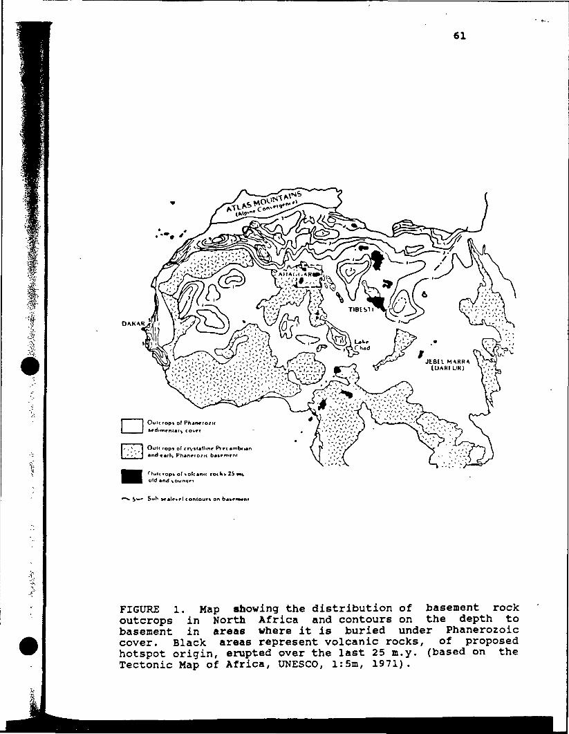
61

DAKAR

Outcrops of Phanrro/Ktrdimrnlary cover

Oulr rop* of crystalline Pr f(• nd carlv Ph«nrio/il b*tf rr*

^>u1< rop» of vo lc<uld and vounqrr

FIGURE l. Map showing the distribution of basement rockoutcrops in North Africa and contours on the depth tobasement in areas where it is buried under Phanerozoiccover. Black areas represent volcanic rocks, of proposedhotspot origin, erupted over the last 25 m.y. (based on theTectonic Map of Africa, UNESCO, l:5m, 1971).

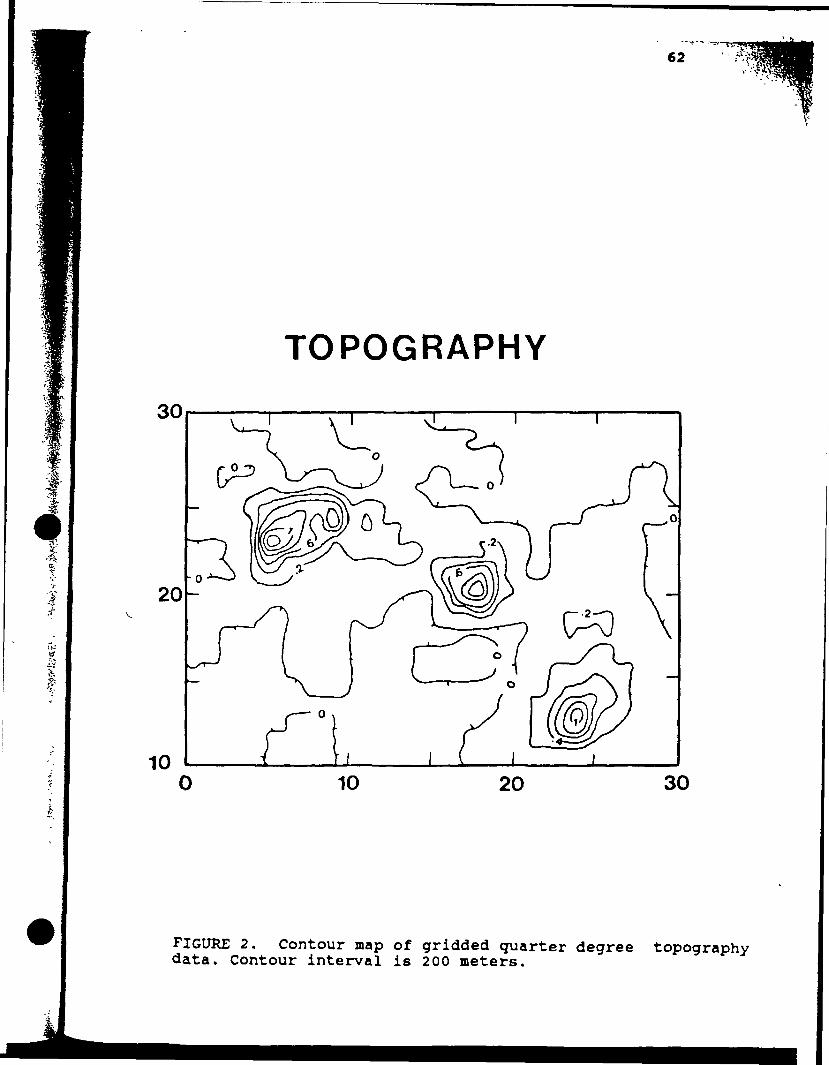
TOPOGRAPHY

62

I

30

20

1010 20 30

FIGURE 2. Contour map of gridded quarter degree topographydata. Contour interval is 200 meters.

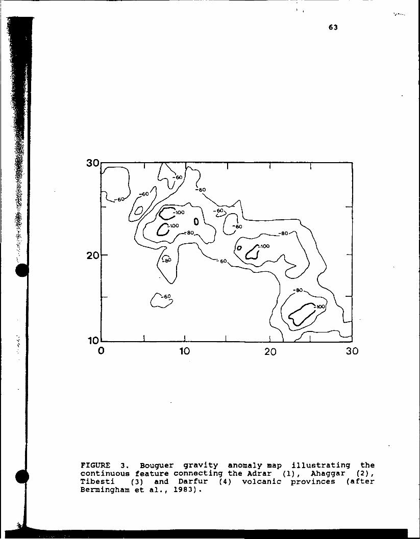
63

30

20

1010 20 30

FIGURE 3. Bouguer gravity anomaly map illustrating thecontinuous feature connecting the Adrar (1), Ahaggar (2),Tibesti (3) and Darfur (4) volcanic provinces (afterBermingham et al., 1983).

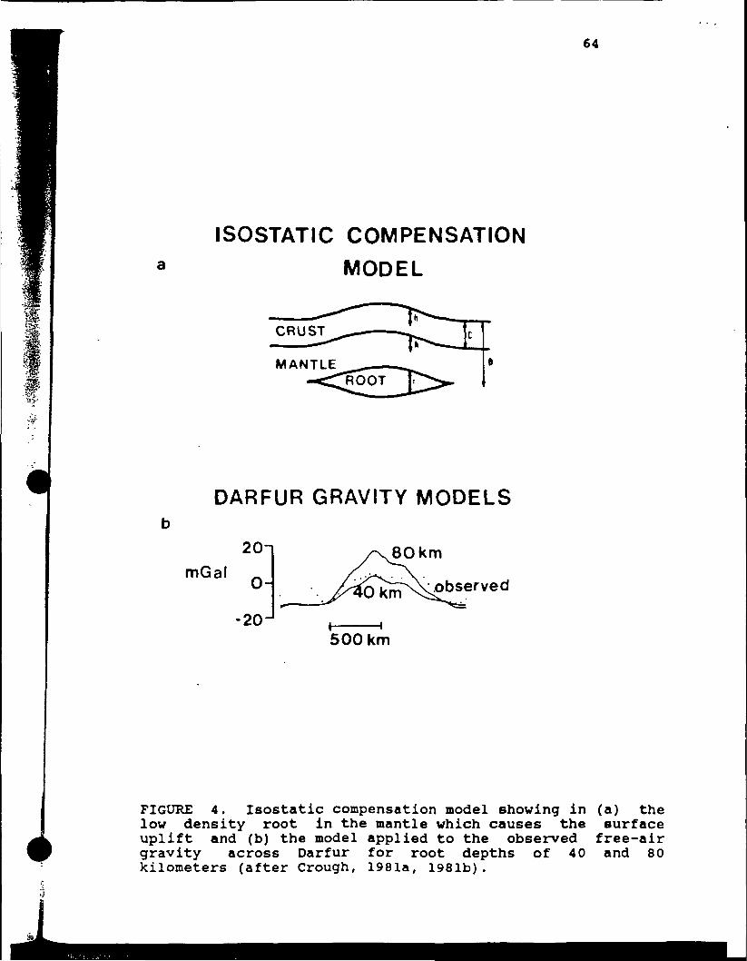
64

ISOSTATIC COMPENSATION

MODEL

DARFUR GRAVITY MODELS

mGal20-

O-

-20 500km

FIGURE 4. Isostatic compensation model showing in (a) thelow density root in the mantle which causes the surfaceuplift and (b) the model applied to the observed free-airgravity across Darfur for root depths of 40 and 80kilometers (after Crough, 1981a, 1981b).

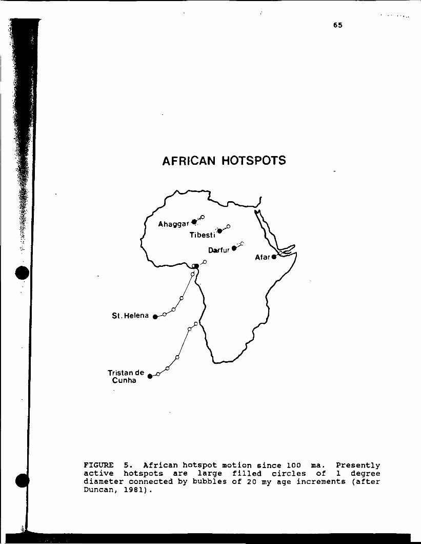
65

AFRICAN HOTSPOTS

St. Helena

Tristan deCunha

FIGURE 5. African hotspot motion since 100 ma. Presentlyactive hotspots are large filled circles of 1 degreediameter connected by bubbles of 20 my age increments (afterDuncan, 1981).

FIGURE 6.

Published Magsat scalar anomaly map (after Langel et al.,1982a).

.1•

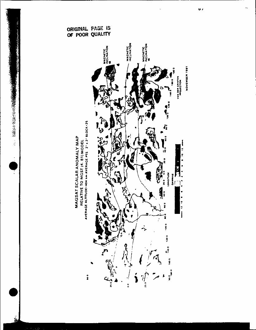
u /

ORIGINAL PAGE iSOF POOR QUALFTY

FIGURE 7

Published Magsat vertical anomaly map (after Langel et al.,1982b).

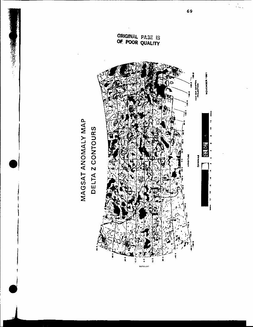
69

ORIGINALPOOR QUALFTY

Scalar magneticStrangway, 1984b).

FIGURE 8.

anomaly map (after Arkani-Hamed and

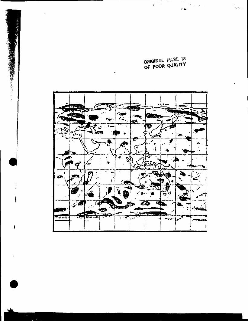
POOR QUALITY

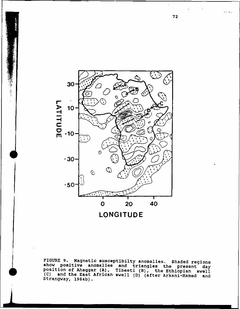
72

-50-

0 20 40

LONGITUDE

FIGURE 9. Magnetic susceptibilty anomalies. Shaded regionsshow positive anomalies and triangles the present dayposition of Ahaggar (A), Tibesti (B), the Ethiopian swell(C) and the East African swell (D) (after Arkani-Hamed andStrangway, 1984b).

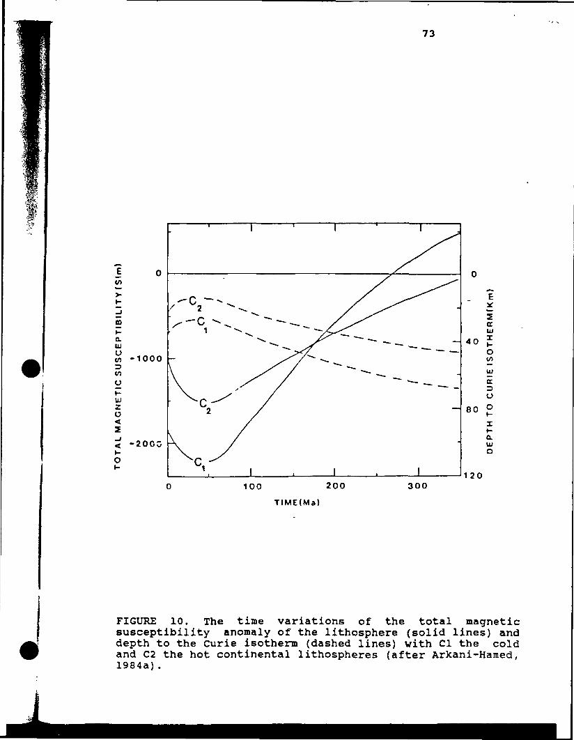
73

- 40

5crtuXt-oto

UJ

aDO

aUJo

120100 200

TIME(Ma)

300

FIGURE 10. The time variations of the total magneticsusceptibility anomaly of the lithosphere (solid lines) anddepth to the Curie isotherm (dashed lines) with Cl the coldand C2 the hot continental lithospheres (after Arkani-Hamed,1984a).

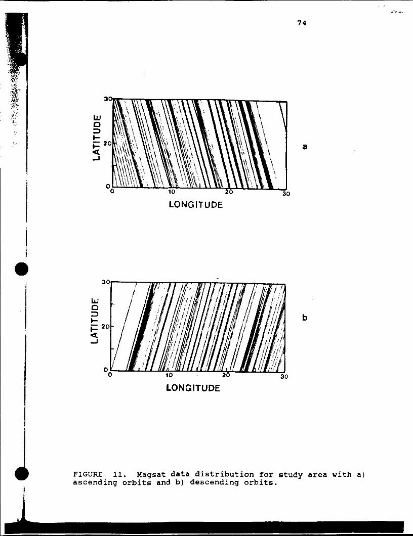
LONGITUDE

74

a

0 toLONGITUDE

30

FIGURE 11. Magsat data distribution for study area with a)ascending orbits and b) descending orbits.

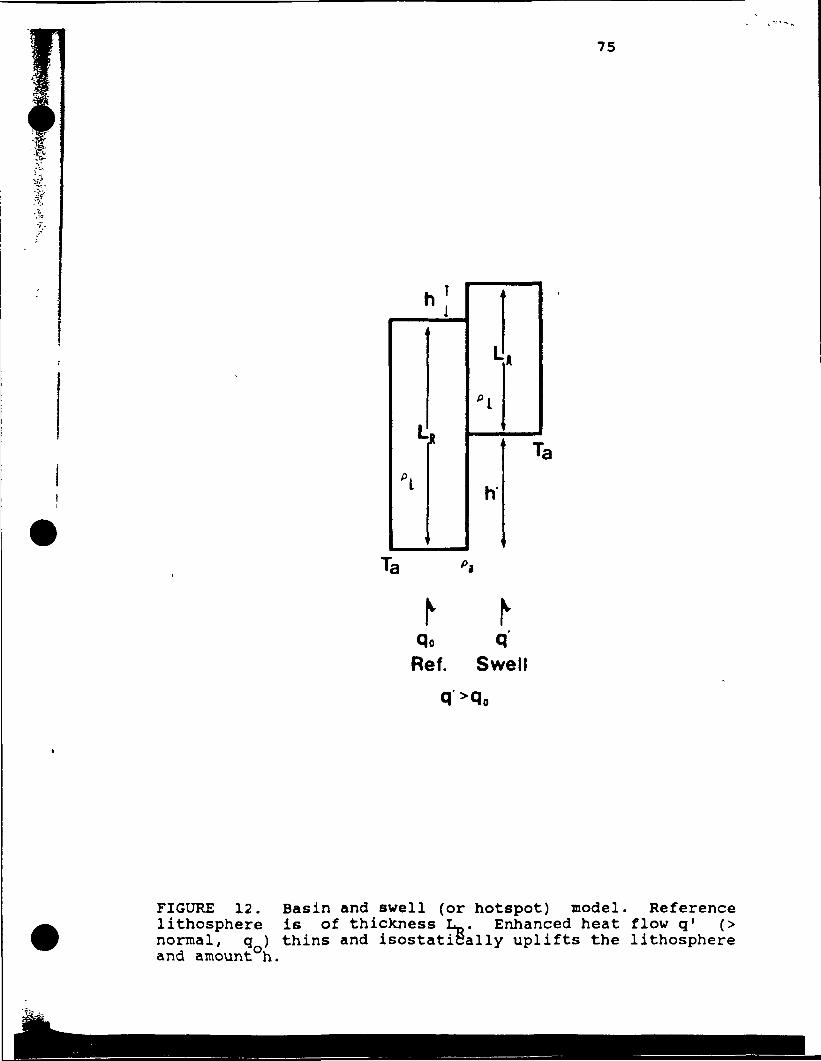
75

h!1

1

Pl

\

I

"I1

i

h

A

Ta

Qo qRef. Swell

FIGURE 12. Basin and swell (or hotspot) model. Referencelithosphere is of thickness L_. Enhanced heat flow q' (>normal, q ) thins and isostatically uplifts the lithosphereand amount°h.

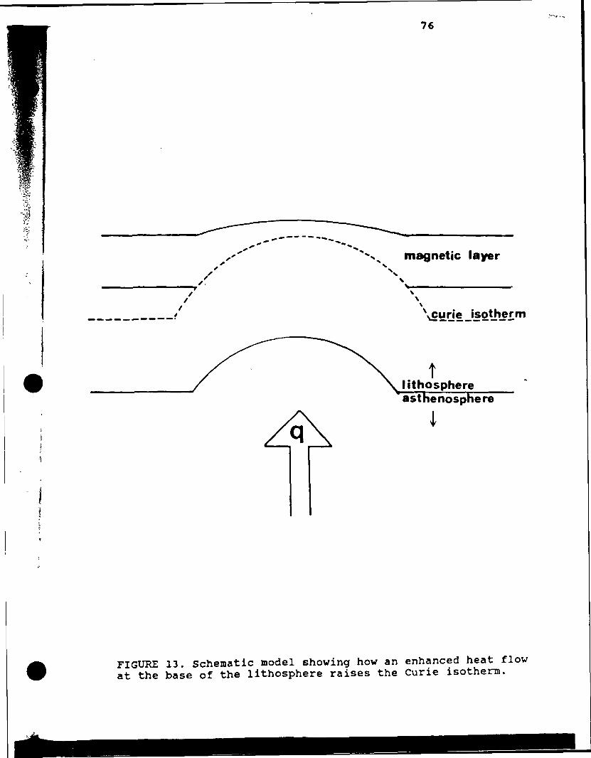
76

magnetic layer

\curie isotherm

tlithosphereasthenosphere

I

FIGURE 13. Schematic model showing how an enhanced heat flowat the base of the lithosphere raises the Curie isotherm.

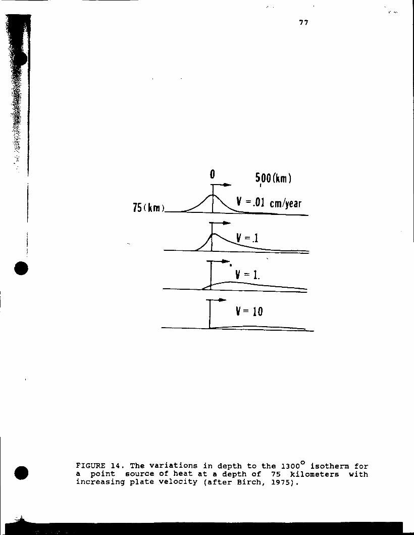
77

75 (km).

0 500 (km)

V =.01 cm/year

V = 1 0

FIGURE 14. The variations in depth to the 1300° isotherm fora point source of heat at a depth of 75 kilometersincreasing plate velocity (after Birch, 1975).

with

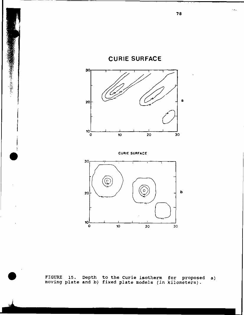
78

CURIE SURFACE

f

30

20

1010 20 30

30

20

10

CURIE SURFACE

10 20 30

FIGURE 15. Depth to the Curie isotherm for proposed a)moving plate and b) fixed plate models (in kilometers).

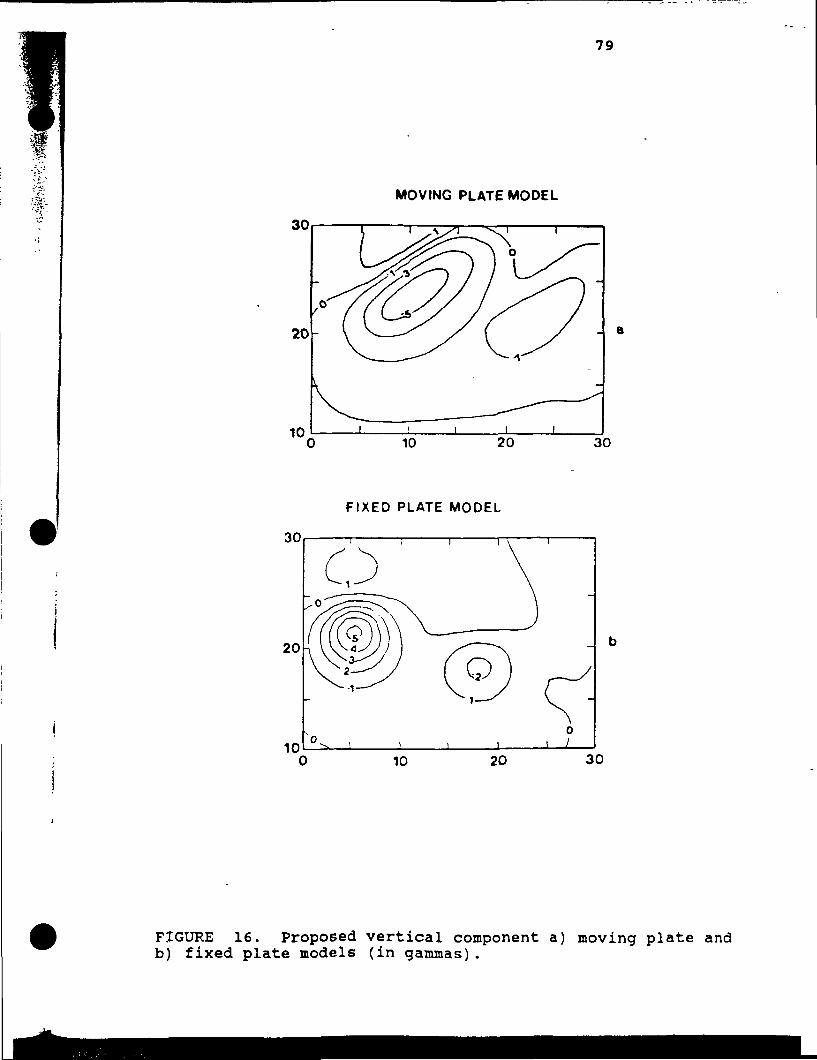
79

1 j '

MOVING PLATE MODEL

30

20

10 i i10 20 30

FIXED PLATE MODEL

10

FIGURE 16. Proposed vertical component a) moving plate andb) fixed plate models (in gammas).

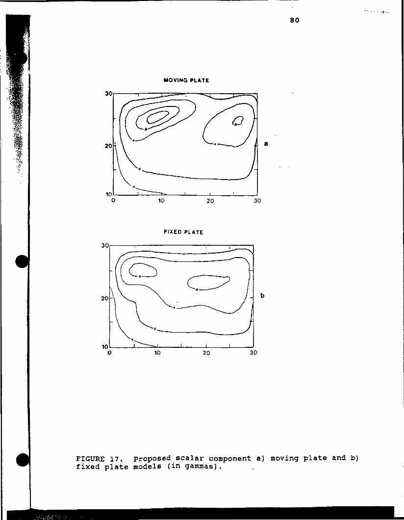
80

MOVING PLATE

30

20

1010 20

a

30

FIXED PLATE

•FIGURE 17. Proposed scalar component a) moving plate and b)fixed plate models (in gammas).

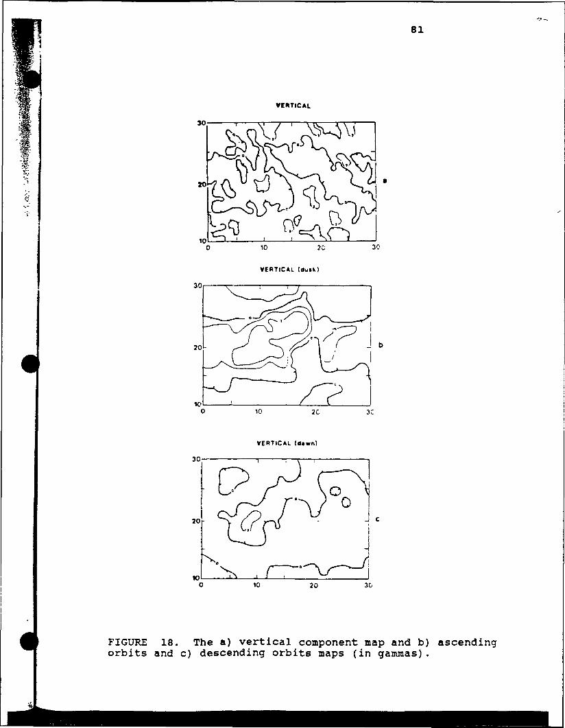
81

1!? »

VERTICAL

VERTICAL (dutk)

1C

J b

VERTICAL (lUwn)

1O

J C

FIGURE 18. The a) vertical component map and b) ascendingorbits and c) descending orbits maps (in gammas).

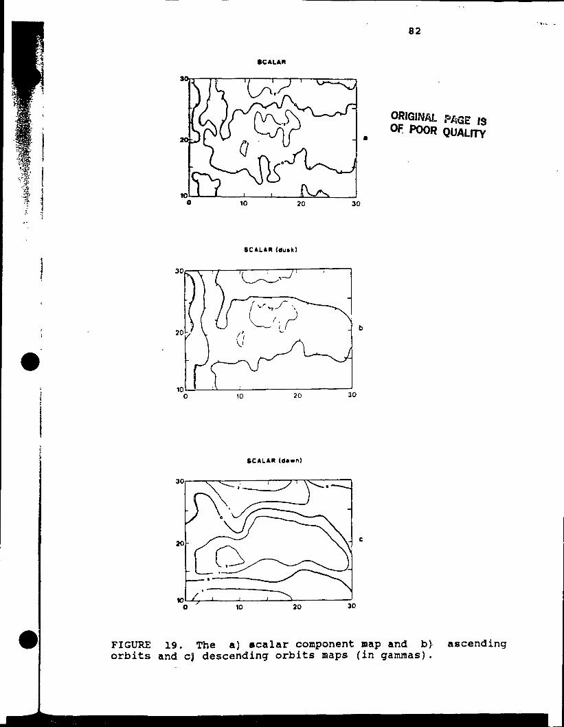
82

SCALAR

1O

ORIGINAL PAGE 13OF POOR QUALITY

SCALAR (duck)

SCALAR (dawn)

4 c

10

FIGURE 19. The a) scalar component map and b) ascendingorbits and c) descending orbits maps (in ganunas) .

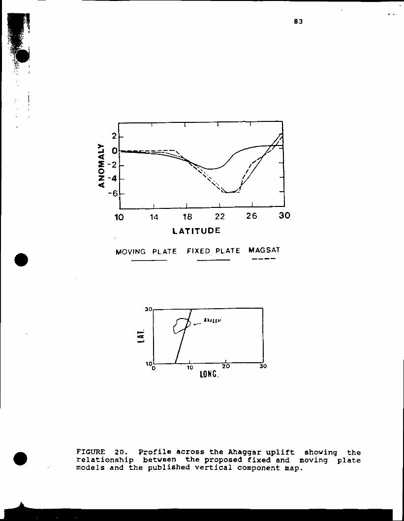
83

10 14 18 22

LATITUDE

MOVING PLATE FIXED PLATE MAGSAT

30

10 10 20

LONG.30

FIGURE 20. Profile across the Ahaggar uplift showing therelationship between the proposed fixed and moving platemodels and the published vertical component map.

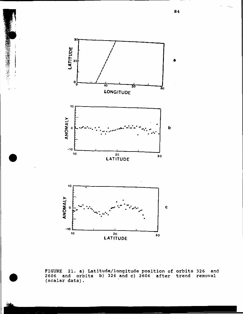
UJof-

20

84

LONGITUDE

10

5 0OZ

-1010

_L

20

LATITUDE30

10

S o

-10 _L10 20

LATITUDE30

FIGURE 21. a) Latitude/longitude position of orbits 326 and2606 and orbits b) 326 and c) 2606 after trend removal(scalar data).

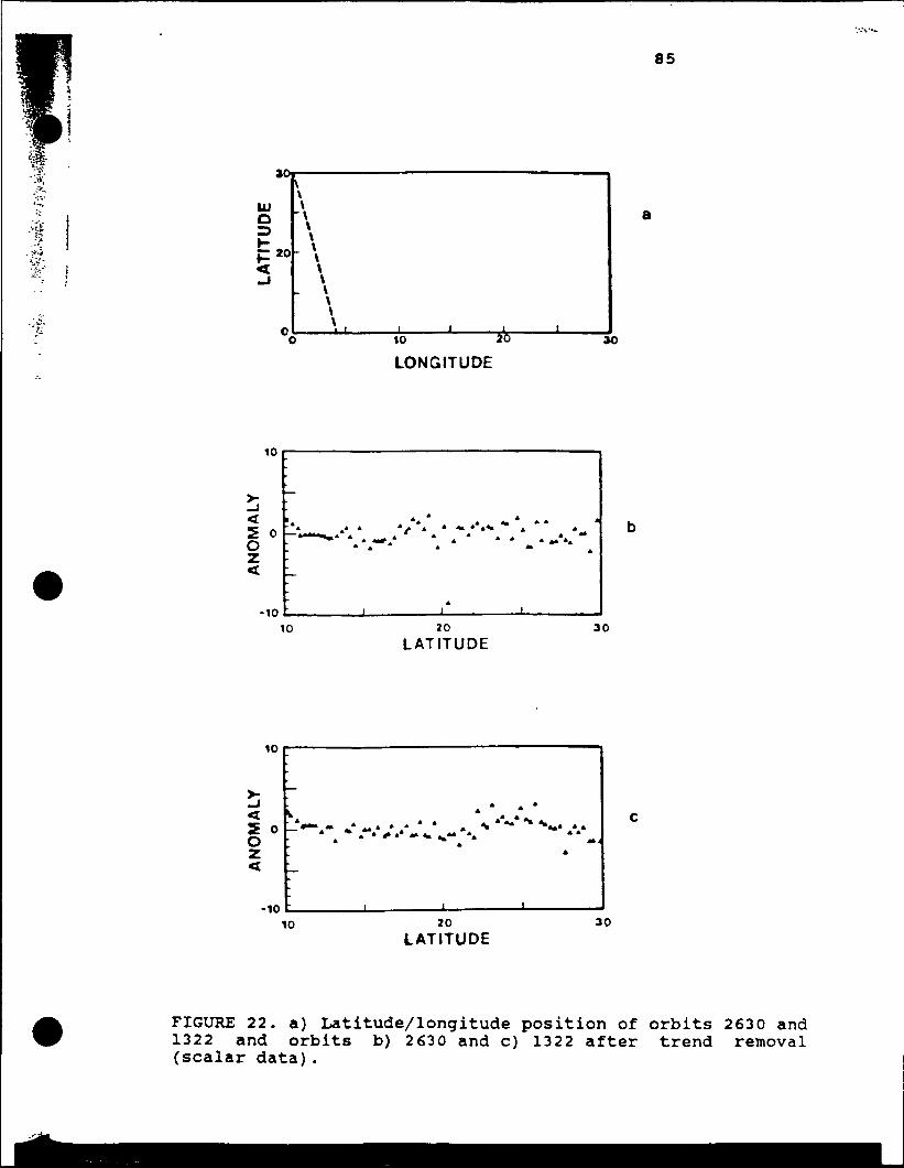
85

»0

IUo=3fc»

^20<_J

0

VV\

• \\

\\\\\\\ ,

10

LONGITUDE3O

10

5 oOz

-1010 20

LATITUDE30

10

OZ

-10

V *_*— - fc* -••*'• « ^ *"-*** *»*.. *»» t */••*«»•- v v- *.

10 20

LATITUDE30

FIGURE 22. a) Latitude/longitude position of orbits 2630 and1322 and orbits b) 2630 and c) 1322 after trend removal(scalar data).

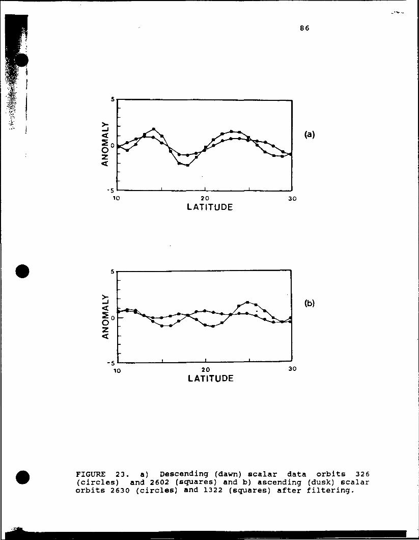
86

<

1°<

-5

(a)

10 20

LATITUDE30

<

1°<

-5

(b)

10 20

LATITUDE30

FIGURE 23. a) Descending (dawn) scalar data orbits 326(circles) and 2602 (squares) and b) ascending (dusk) scalarorbits 2630 (circles) and 1322 (squares) after filtering.

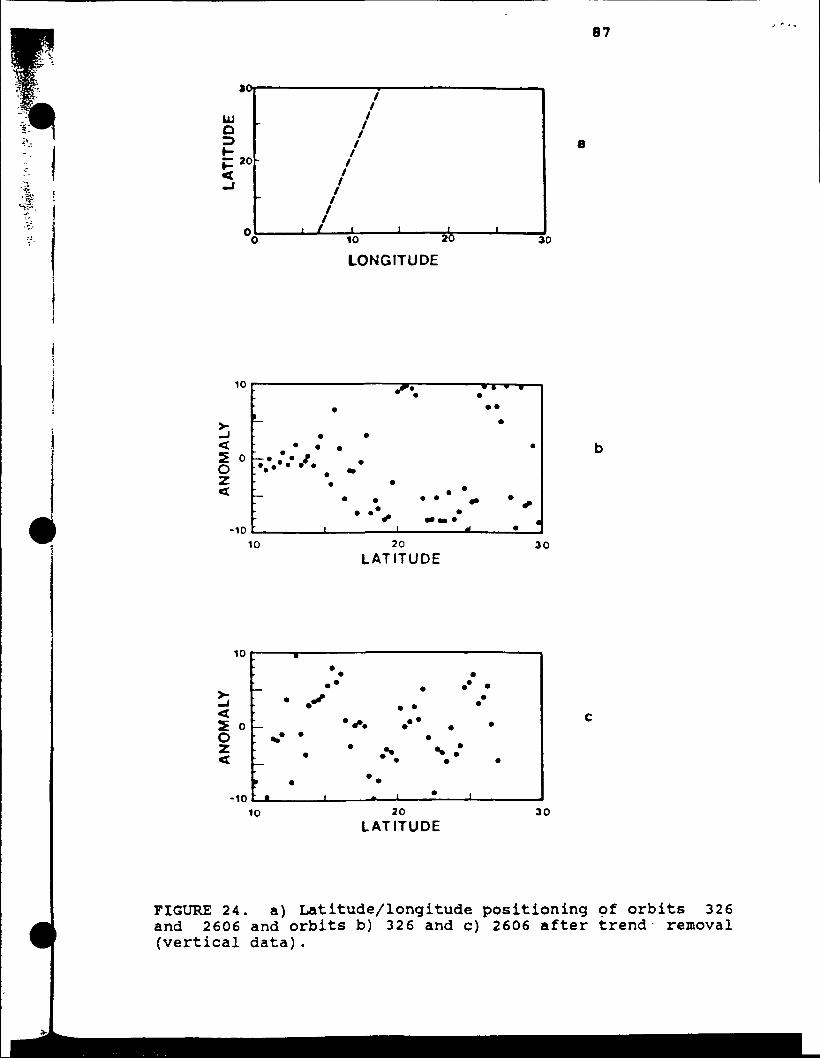
UJ0

87

a

to 20

LONGITUDE30

10

Or

-1010

• • ••

20LATITUDE

10

Oz

-10

10 20LATITUDE

30

FIGURE 24. a) Latitude/longitude positioning of orbits 326and 2606 and orbits b) 326 and c) 2606 after trend removal(vertical data).

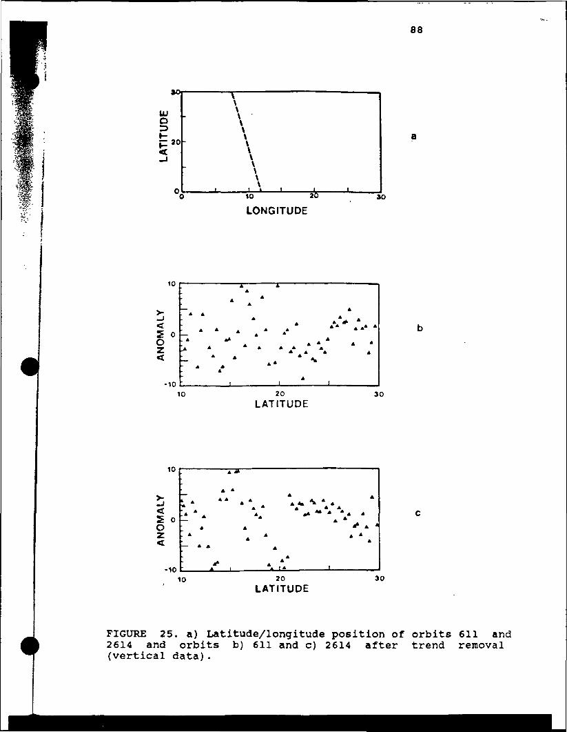
88

UJol >

^20

_J

O

\\\V\\\\\\\\1 I I I 1 1

a

10 20

LONGITUDE

10

OZ

-10

AA

10 20LATITUDE

30

10

>-_J<S oOz<

-10

A A*

A »

'A ** A * * *A * *

** * A *»A* ********* A A

A A ^ A 4

*

- * * A

A

- A * * 1 * * I * 1

10 20

LATITUDE30

FIGURE 25. a) Latitude/longitude position of orbits 611 and2614 and orbits b) 611 and c) 2614 after trend removal(vertical data).

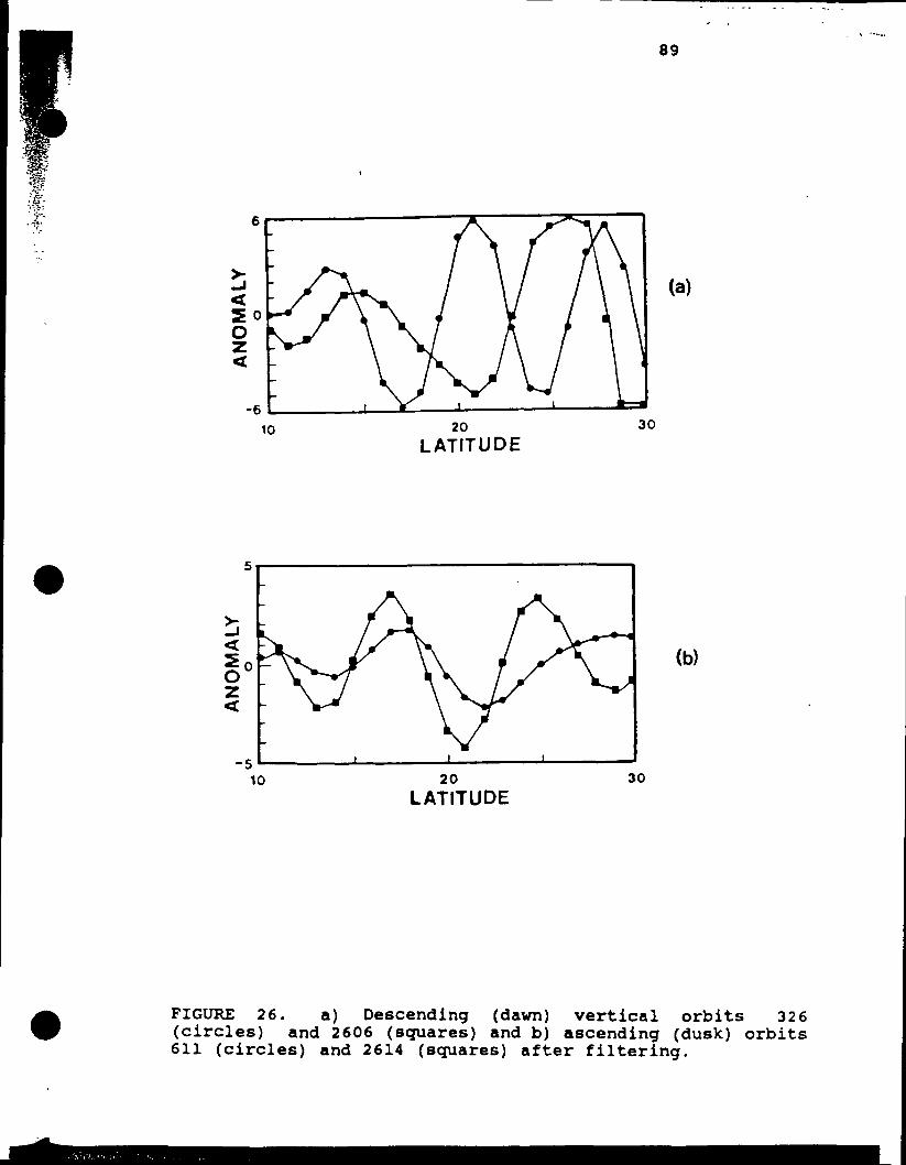
89

(a)

-610 20

LATITUDE

<

§°

-5

(b)

10 20LATITUDE

30

FIGURE 26. a) Descending (dawn) vertical orbits 326(circles) and 2606 (squares) and b) ascending (dusk) orbits611 (circles) and 2614 (squares) after filtering.

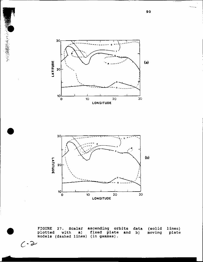
90

(a)

10 20LONGITUDE

3 20-

om

(b)

10 20LONGITUDE

FIGURE 27. Scalar ascending orbits data (solid lines)plotted with a) fixed plate and b) moving platemodels (dashed lines) (in gammas).

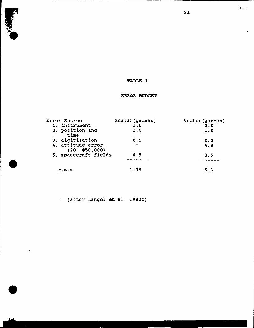
91

TABLE 1

ERROR BUDGET

Error Source1. instrument2. position and

time3. digitization4. attitude error

(20" £50,000)5. spacecraft fields

Scalar(gammas)1.51.0

0.5

0.5

Vector(gammas)3.01.0

0.54.8

0.5

r. s. s 1.96 5.8

(after Langel et al. 1982c)

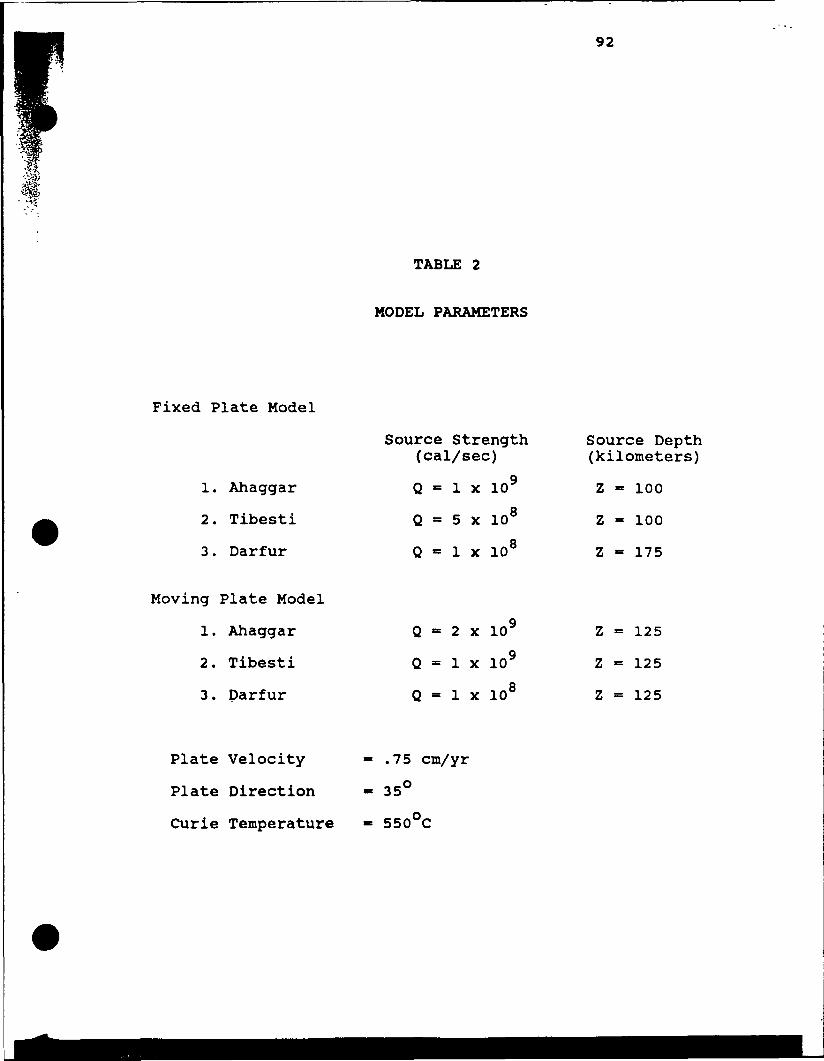
TABLE 2

MODEL PARAMETERS

92

Fixed Plate Model

1. Ahaggar

2. Tibesti

3. Darfur

Moving Plate Model

1. Ahaggar

2. Tibesti

3. Darfur

Source Strength(cal/sec)

Q

Q

Q

1 x 10'

5 x 10'

1 x 10

2 x 10'

Q = 1 x ID"

1 x 10

Source Depth(kilometers)

Z = 100

Z « 100

Z «= 175

Z = 125

Z = 125

Z = 125

Plate Velocity

Plate Direction

Curie Temperature

.75 cm/yr

35°

550°C

93

REFERENCES

Arkani-Hamed, J. and Strangway, D. W., 1984a, Aninterpretation of the magnetic signatures ofaulacogens and cratons in Africa and South America,(submitted to) Tectonophysics.

Arkani-Hamed, J. and Strangway, D. W., 1984b, Lateralvariations of apparent magnetic susceptibility oflithosphere deduced from MAGSAT data, (submitted to)Journal of Geophysical Research.

Bermingham, P.M., Fairhead, J.D. and Stuart, G.W., 1983,Gravity study of the central African rift system: amodel of continental disruption, Tectonophysics, 94,205-222.

Birch, Francis S., 1975, Conductive heat flow anomalies overa hotspot in a moving medium, Journal ofGeophysical Research, 80, 4825-4827.

Black, R, and Girod, M., 1970, Late Paleozoic to Recentigneous activity in West Africa and its relationshipto basement structures, in African Magmatismand Tectonics, ed. Clifford, T.N.Hafner Pub. Co., Conneticut, 185-210.

and Gass, I.G.,

Briden, J.C. and Gass, I.G., 1974, Plate movement andcontinental magmatism, Nature, 248, 650-653, 1974.

Brown, C., Girdler, R.W. and Renner, R.G.B., 1980, A gravitytraverse across Northern Africa, Journal ofGeophysical Research, 85, 6436-6442.

Brown, C. and Girdler, R.W., 1980, Interpretation of Africangravity and its implication for the breakup ofthe continents, Journal of Geophysical Research,8J5, 6443-6455.

Browne, S.E. and Fairhead, J.D.,1983,Gravity study of thecentral African rift system: a model for continentaldisruption 1. the Ngaoundere and Abu Gabra rifts,Tectonophysics, 94, 187-203.

94

Burke, K. and Dewey, J.F., 1974, Two plates in Africa duringthe Cretaceous ?, Nature, 249, 313-316.

Burke, K., Kidd, W.S.F. and Wilson, J. Tuzo, 1973, Relativeand latitudinal motion of Atlantic hot spots,Nature, 245, 133-137.

Burke, K. and Wilson, J.T., 1972, Is the African platestationary?, Nature, 239, 387-389.

Chase, Clement G., 1978, Plate kinematics: the Americas,East Africa, and the rest of the world, Earth andPlanetary Science Letters, 37, 355-368.

Coney, Peter J., 1977, Mesozoic and Cenozoic Cordilleranplate tectonics, Geological Society of America Memoir152, 33-50.

Crough, S. Thomas, 198la, The Darfur swell, Africa: gravityconstraints on its isostatic compensation, Geophys.Res. Let., 8, 877-879.

Crough, S. Thomas, 1981b, Free-air gravity over the HoggarMassif, northwest Africa: evidence for the alterationof the lithosphere, Tectonophysics, 77, 189-202.

Crough, S. Thomas, 1979, Hotspot epeirogeny, Tectonophysics,61, 321-333.

Crough, S. Thomas, 1978, Thermal origin of mid-platehotspot swells, Geophys. J. R. astr. Soc., 55, 452-469.

Duncan, R.A., 1981, Hotspots in the southern oceans-anabsolute frame of reference for motion of the Gondwanacontinents, Tectonophysics, 74, 29-42.

Fairhead, J.D., 1980, The intra-plate volcanic centres ofNorth Africa and their possible relation to the EastAfrican rift system, Atti dei Convengni Zincei, 47-48.

Fairhead, J.D., 1979, A gravity link between the domallyuplifted Cainozoic volcanic centres of North Africaand its similarities to the East African riftsystem anomaly, Earth and Planetary Science Letters,4_2, 109-113.

Fairhead, J.D. and Girdler, R.W., 1971, The seismicity ofAfrica, Geophys. J. R. astr. Soc., 24, 271-301.

Fairhead, J.D. and Reeves, C.V., 1977, Teleseismic delaytimes, anomalies and inferred thickness of the Africanlithosphere, Earth and Planetary Science Letters, 3663-76.

95

Francis, P.W., Thorpe, R.S. and Ahmed, F., 1973, Setting andsignificance of Tertiary to Recent volcanism in theDarfur province of Western Sudan, Nature PhysicalScience, 243, 30-32.

Galliher, S.C. and Mayhew, M.A., 1982, On thepossibility of detecting large-scale crustal remanentmagnetization with MAGSAT vector anomaly data,Geophysical Research Letters, 9_, 325-328.

Gass, I.G., Chapman, D.S., Pollack, H.N. and Thorpe, R.S,1978, Geologic and geophysical parameters of mid-platevolcanism, Phil. Trans. Soc. Lond. A, 288, 581-597.

Girdler, R.W. and Styles, P., 1974, Two stage Red Sea floorspreading, Nature, 247, 7-10.

Haggerty, Stephen E., 1978, Mineralogical constraints onCurie isotherms in deep crustal magneticanomalies, Geophysical Research Letters, 5^, 105-108.

Hastings, David A., 1982, Preliminary correlations of MAGSATanomalies with tectonic features in Africa,Geophysical Research Letters, 9_, 303-306.

Jain, Birendra K. and Regan, Robert D., 1982, Integration ofsatellite and conventional geophysical data withtectonic and structural information over theAfrican continent, Geoexploration, 20, 233-258.

LaBrecgue, J.L. and Cande, S.C., 1984, Intermediatewavelength magnetic anomalies over the centralPacific, Journal of Geophysical Research , 89, B13,11124-11134.

Langel, R.A., 1982, The magnetic earth as seen from MAGSAT,initial results, Geophysical Research Letters, £,239-242.

Langel, R.A. and Estes, R.H., 1982, A geomagnetic fieldspectrum, Geophysical Research Letters, 9_, 250-253.

Langel, R.A., Phillips, J.D. and Horner, R.J., 1982a,Initial scalar magnetic anomaly map from MAGSAT,Geophysical Research Letters, 9^, 269-272.

Langel, R.A., Schnetzler, C.C., Phillips, J.D. and Horner,R.J., 1982b, Initial vector magnetic anomaly map fromMAGSAT, Geophysical Research Letters, 9, 273-298.

Langel, R.A., Ousley, Gilbert, Berbert, John, Murphy, Jamesand Settle, Mark, 1982c, The MAGSAT mission,Geophysical Research Letters, 9, 243-245.

Maeda, H., lyemori, T., Araki, T. and Kamei, T., 1982, Newevidence of a meridional current system in the

equatorial ionosphere,9, 337-340.

96

Geophysical Research Letters,

McKenzie, Dan and Sclater, John G., 1971, The evolution ofthe Indian Ocean since the late Cretaceous, Geophys.J. R. astr. Soc., 25, 437-528.

Morgan, J.W., 1972, Deep mantle convection plumes and platemotion, American Association of Petroleum GeologistsBulletin, 56, 203-213.

Parker, R.L., 1972, The rapid calculation of potentialanomalies, Geophys. J. R. astr. Soc., 31, 447-455.

Regan Robert D. and Marsh, Bruce D., 1982, The Banguimagnetic anomaly: its geological origin, Journal ofGeophysical Research, 87, 1107-1120.

Sailor, R.V., Lazarewicz, A.R. and Brammer, R.F., 1982,Spatial resolution of MAGSAT crustal anomaly data overthe Indian Ocean, Geophysical Research Letters, £,289-292.

Vail, J.R., 1970, Tectonic control of dykes and relatederruptive rocks in Eastern Africa, in African Magmatismand Tectonics, ed. Clifford, T.N. and Gass, I.G.,Hafner Pub. Co., Conneticut, 337-354.

Vincent, P.M., 1970, The evolution of Tibesti volcanicprovince, Eastern Sahara, in African Magmatism andand Tectonics, ed. Clifford, T.N. and Gass, I.G.,Hafner Pub. Co., Conneticut, 301-320.

Wasilewski, Peter J., Thomas, Herman H. and Mayhew, M.A.,1979, The MOHO as a magnetic boundary, GeophysicalResearch Letters, £, 541-544.

Wilson, J.100.

T., 1963, Continental drift, Sci. Am., 208, 86-

Yee-han Ng, Carolyn, 1983, Combined use of wavenumberanalysis of Landsat digital imagery and seismic datato infer the orientation of tectonic stress in theHoggar region of Africa, Master of ScienceThesis, Pennslyvania State^Univ., 12Op.