Embed Size (px)
Citation preview

Space = Time 9 Matter Modern Kaluza-Klein Theory

Space - Time 9 Matter Modern Kaluza-Klein Theory
Paul S Wesson University of Waterloo, Ontario, Canada and
Hansen Physics Labs, Stanford University
World Scientific Singapore New Jersey. London Hong Kong
Published by
World Scientific Publishing Co. Re. Ltd. P 0 Box 128, Famr Road, Singapore 912805 USA officer Suite lB, 1060 Main Street, River Edge, NJ 07661 UK ofice: 57 Shelton Street, Covent Garden, London WC2H 9HE
British Library Cataloguing-in-Publication Data A catalogue record for this book is available from the British Library.
SPACE, TIME, MATTER: MODERN KALUZA-KLEIN THEORY Copyright Q 1999 by World Scientific Publishing Co. Re. Ltd. All rights reserved. This book, or parts thereof, may not be reproduced in any form or by any means, electronic or mechanical, includingphotocopying, recording or any information storage and retrieval system now known or to be invented, without written permission from the Publisher.
For photocopying of material in this volume, please pay a copying fee through the Copyright Clearance Center, Inc., 222 Rosewood Drive, Danvers, MA 01923, USA. In this case permission to photocopy is not required from the publisher.
ISBN 981-02-3588-7
Printed in Singapore.
PREFACE
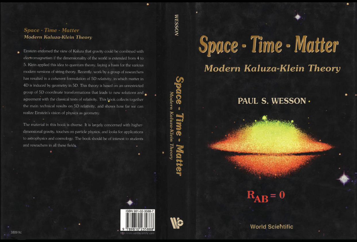
Einstein endorsed the view of Kaluza, that gravity could be combined with
electromagnetism if the dimensionality of the world is extended from 4 to 5. Klein applied this
idea to quantum theory, laying a basis for the various modem versions of string theory.
Recently, work by a group of researchers has resulted in a coherent formulation of 5D relativity,
in which matter in 4D is induced by geometry in 5D. This theory is based on an unrestricted
group of 5D coordinate transformations that leads to new solutions and agreement with the
classical tests of relativity. This book collects together the main technical results on 5D
relativity, and shows how far we can realize Einstein’s vision of physics as geometry.
Space, time and matter are physical concepts, with a long but somewhat subjective
history. Tensor calculus and differential geometry are highly developed mathematical
formalisms. Any theory which joins physics and algebra is perforce open to discussions about
interpretation, and the one presented in this book leads to new issues concerning the nature of
matter. The present theory should not strictly speaking be called Kaluza-Klein: KK theory relies
on conditions of cylindricity and compactification which are now removed. The theory should
also. while close to it in some ways, not be confused with general relativity: GR theory has an
explicit energy-momentum tensor for matter while now there is none. What we call matter in 4D
spacetime is the manifestation of the fifth dimension, hence the phrase induced-matter theory
sometimes used in the literature. However, there is nothing sacrosanct about 5D. The field
equations take the same form in ND, and N is to be chosen with a view to physics. Thus,
superstrings (10D) and supergravity (1lD) are valid constructs. However, practical physical
applications are expected to be forthcoming only if there is physical understanding of the nature
of the extra dimensions and the extra coordinates. In this regard, space-time-matter theory is
V
vi Preface
uniquely fortunate. This because (unrestricted) 5D Riemannian geometry turns out to be just
algebraically rich enough to unify gravity and electromagnetism with their sources of mass and
charge. In other words, it is a Machian theory of mechanics.
There is now a large and rapidly growing literature on this theory, and the author is aware
that what follows is more like a textbook on basics than a review of recent discoveries. It should
also be stated that much of what follows is the result of a group effort over time. Thus credit is
due especially to H. Liu, B. Mashhoon and J. Ponce de Leon for their solid theoretical work; to
C.W.F. Everitt who sagely kept us in contact with experiment; and to A. Billyard, D. Kalligas,
J.M. Overduin and W. Sajko, who as graduate students cheerfully tackled problems that would
have made their older colleagues blink. Thanks also go to S. Chatterjee, A. Coley, T. Fukui and
R. Tavakol for valuable contributions. However, the responsibility for any errors or omissions
rests with the author.
The material in this book is diverse. It is largely concerned with higher-dimensional
gravity, touches particle physics, and looks for application to astrophysics and cosmology.
Depending on their speciality, some workers may not wish to read this book from cover to cover.
Therefore the material has been arranged in approximately self-contained chapters, with a
bibliography at the end of each. The material does, of course, owe its foundation to Einstein.
However, it will be apparent to many readers that it also owes much to the ideas of his
contemporary, Eddington.
Paul S. Wesson

CONTENTS
Preface
ConceDts and Theories of Phvsics
Introduction Fundamental Constants General Relativity Particle Physics Kaluza-Klein Theory Supergravity and Superstrings Conclusion
bduced-Matter Theory
Introduction A 5D Embedding for 4D Matter The Cosmological Case The Soliton Case The Case of Neutral Matter Conclusion
V
1.
1.1 1.2 1.3 1.4 1.5 1.6 1.7
2.
2.1 2.2 2.3 2.4 2.5 2.6
3.
3.1 3.2 3.3 3.4 3.5 3.6 3.7 3.8
4.
4.1 4.2 4.3 4.4 4.5 4.6 4.7 4.8
The Classical and Other Tests in 5D
Introduction The 1-Body Metric Photon Orbits Particle Orbits The Redshift Effect The Geodetic Effect and GP-B The Equivalence Principle and STEP Conclusion
Cosmolorrv and Astroohvsics in 5D
Introduction The Standard Cosmological Model Spherically-S ymmetric Astrophysical Systems Waves in a de Sitter Vacuum Time-Dependent Solitons Systems with Axial and Cylindrical Symmetry Shell-Like and Flat Systems Conclusion
1
1 2 11 18 28 33 37
42
42 43 44 49 58 66
69
69 69 72 77 81 82 85 88
91
91 92 105 108 111 114 117 125
vii
viii
5.
5.1 5.2 5.3 5.4 5.5 5.6 5.7
6.
6.1 6.2 6.3 6.4 6.5 6.6 6.7
7.
7.1 7.2 7.3 7.4 7.5 7.6 7.7
8.
Content3
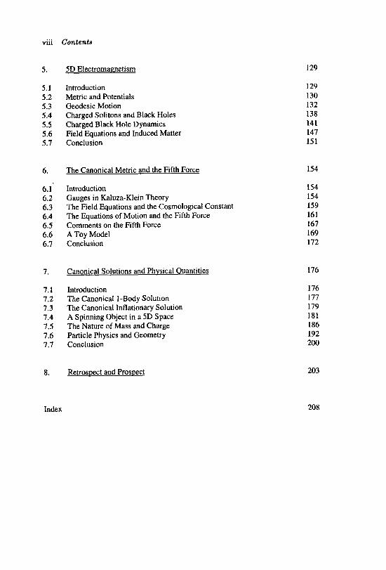
5D Electromagnetism
Introduction Metric and Potentials Geodesic Motion Charged Solitons and Black Holes Charged Black Hole Dynamics Field Equations and Induced Matter Conclusion
The Canonical Metric and the Fifth Force
Introduction Gauges in Kaluza-Klein Theory The Field Equations and the Cosmological Constant The Equations of Motion and the Fifth Force Comments on the Fifth Force A Toy Model Conclusion
Canonical Solutions and Phvsical Ouantities
Introduction The Canonical 1-Body Solution The Canonical Inflationary Solution A Spinning Object in a 5D Space The Nature of Mass and Charge Particle Physics and Geometry Conclusion
Retrospect and Prospect
129
129 130 132 138 141 147 151
154
154 154 159 16 1 167 169 172
176
176 177 179 181 186 192 200
203
Index 208
1, CONCEPTS AND THEORIES OF PHYSICS
“Physics should be beautiful” (Sir Fred Hoyle, Venice, 1974)
1.1 Introduction
Physics is a logical activity, which unlike some other intellectual pursuits frowns on
radical departures, progressing by the introduction of elegant ideas which give a better basis for
what we already know while leading to new results. However, this inevitably means that the
subject at a fundamental level is in a constant state of reinterpretation. Also, it is often not easy
to see how old concepts fit into a new framework. A prime example is the concept of mass,
which has traditionally been regarded as the source of the gravitational field. Historically, a
source and its field have been viewed as separate things. But as recognized by a number of
workers through time, this distinction is artificial and leads to significant technical problems.
Our most successful theory of gravity is general relativity, which traditionally has been
formulated in terms of a set of field equations whose left-hand side is geometrical (the Einstein
tensor) and whose right-hand side is material (the energy-momentum tensor). However, Einstein
himself realized soon after the formulation of general relativity that this split has drawbacks, and
for many years looked for a way to transpose the “base-wood” of the right-hand side of his
equations into the “marble” of the left-hand side. Building on ideas of Kaluza and Klein, it has
recently become feasible to realize Einstein’s dream, and the present volume is mainly a
collection of technical results, which shows how this can be done. The basic idea is to unify the
source and its field using the rich algebra of higher-dimensional Riemannian geometry. In other
words: space, time and matter become parts of geometry.
This is an idea many workers would espouse, but to be something more than an academic
jaunt we have to recall the two conditions noted above. Namely, we have to recover what we
1
2 Space, Time, Matter
already know (with an unavoidable need for reinterpretation); and we have to derive something
new with at least a prospect of testability. The present chapter is concerned with the first of
these, and the succeeding chapters mainly with the second. Thus the present chapter is primarily
a review of gravitation and particle physics as we presently understand these subjects. Since this
is mainly known material, these accounts will be kept brief, and indeed those readers who are
familiar with these subjects may wish to boost through them. However, there is a theme in the
present chapter, which transcends the division of physics into theories of macroscopic and
microscopic scope. This is the nature and origin of the so-called fundamental constants. These
are commonly taken as indicators of what kmd of theory is under consideration (e.g., Newton’s
constant is commonly regarded as typical of classical theory and Planck’s constant as typical of
quantum theory). But at least one fundamental constant, the speed of light, runs through all
modem physical theories; and we cannot expect to reach a meaningful unification of the latter
without a proper understanding of where the fundamental constants originate. In fact, the
chapters after this one make use of a view that it is necessary to establish and may be unfamiliar
to some workers: the fundamental constants are not really fundamental, their main purpose being
to enable us to dimensionally transpose certain material quantities so that we can write down
consistent laws of physics.
1.2 Fundamental Constants
A lot has been written on these, and there is a large literature on unsuccessful searches for
their possible variations in time and space. We will be mainly concerned with their origin and
status, on which several reviews are available. Notably there are the books by Wesson (1978),
Petley (1985) and Barrow and Tipler (1986); the conference proceedings edited by McCrea and
Concepts and Theories of Physics 3
Rees (1983); and the articles by Barrow (1981) and Wesson (1992). We will presume a working
physicist's knowledge of the constants concerned, and the present section is to provide a basis
for the discussions of physical theory which follow.
The so-called fundamental constants are widely regarded as a kind of distillation of
physics. Their dimensions are related to the forms of physical laws, whose structure can in many
cases be recovered from the constants by dimensional analysis. Their sizes for some choice of
units allow the physical laws to be evaluated and compared to observation. Despite their
perceived fundamental nature, however, there is no theory of the constants as such. For
example, there is no generally accepted formalism that tells us how the constants originate, how
they relate to one another, or how many of them are necessary to describe physics. This lack of
backpund seems odd for parameters that are widely regarded as basic.
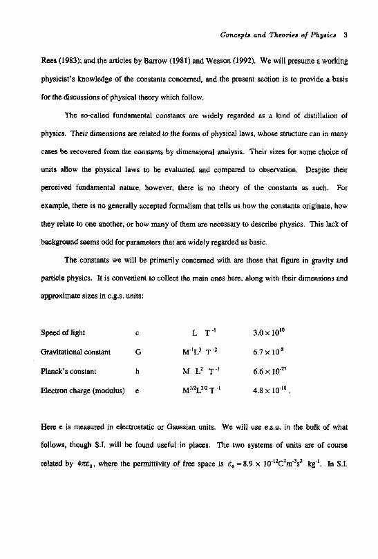
The constants we will be primarily concerned with are those that figure in gravity and
particle physics. It is convenient to collect the main ones here, along with their dimensions and
approximate sizes in c.g.s. units:
Speed of light C
Gravitational constant G
Planck's constant h
Electron charge (modulus) e
L T " 3.0 x 10"
6.7 x lo'*
6.6 x 10''
4.8 x lo-''
~ - 1 ~ 3 T -2
M Lz T - '
~ 1 / 2 ~ 3 / 2 T - I
Here e is measured in electrostatic or Gaussian units. We will use e.s.u. in the bulk of what
follows, though S.I. will be found useful in places. The two systems of units are of course
da ted by 4n&,, where the permittivity of fm space is E, =8.9 x 10~'2CZm'3sZ kg". In S.I.
4 Space, Time, Matter
e = 1.6 x IOl9C (Coulombs: see Jackson 1975, pp. 29, 817; and Griffiths 1987. p. 9). The
permeability of free space p, is not an independent constant because c2 H 1 / &,p0. The above
table suggests that we need to understand 3 overlapping things: constants, dimensions and units.
One common view of the constants is that they define asymptotic states. Thus c is the
maximum velocity of a massive particle moving in flat spacetime; G defines the limiting
potential for a mass that does not form a black hole in curved spacetime; E, is the empty-space
or vacuum limit of the dielectric constant; and h defines a minimum amount of energy
(alternatively A e h / 2a defines a minimum amount of angular momentum). This view is
acceptable, but somewhat begs the question of the constants' origin.
Another view is that the constants are necessary inventions. Thus if a photon moves
away from an origin and attains distance r in time t, it is necessary to write r = ct as a way of
reconciling the different natures of space and time. Or, if a test particle of mass ml moves under
the gravitational attraction of another mass mz and its acceleration is d2r/dtZ at separation r, it is
observed that mld2r/dt2 is proportional to mlmz/rz, and to get an equation out of this it is
necessary to write d2r/dtz = Gm& as a way of reconciling the different natures of mass, space
and time. A similar argument applies to the motion of charged bodies and E , . In quantum
theory, the energy E of a photon is directly related to its frequency V , so we necessarily have to
write E = h v . The point is, that given a law of physics which relates quantities of different
dimensional types, constants with the dimensions c = LT-', G = MlL3T-', E, = Q z M - ' C 3 T 2 and
h = MLV-' are obligatory.
This view of the constants is logical, but disturbing to many because it means they are not
really fundamental and in fact largely subjective in origin. However, it automatically answers
the question raised in the early days of dimensional analysis as to why the equations of physics
Concepts and Theories of Physics 5
are dimensionally homogeneous ( e g Bridgman 1922). It also explains why subsequent attempts
to formalize the constants using approaches such as group theory have led to nothing new
physically (e.g. Bunge 1971). There have also been notable adherents of the view that the
fundamental constants are not what they appear to be. Eddington (1929, 1935, 1939) put
forward the opinion that while an external world exists, our laws are subjective in the sense that
they an constructed to match our own physical and mental modes of perception. Though he was
severely criticized for this opinion by physicists and philosophers alike, recent advances in
particle physics and relativity make it more palatable now than before. Jeffreys (1973, pp. 87-
94, 97) did not see eye to eye with Eddington about the sizes of the fundamental constants, but
did regard some of them as disposable. In particular, he pointed out that in electrodynamics c
merely measures the ratio of electrostatic and electromagnetic units for charge. Hoyle and
Narlikar (1974, pp. 97,98) argued that the c2 in the common relativistic expression (c2t2- xz -
y2 - zz) should not be there, because “there is no more logical reason for using a different time
unit than there would be for measuring x, y, z in different units”. They stated that the velocity of
light is unity, and its size in other units is equivalent to the definition 1 s = 299 792 500 m, where
the latter number is manmade. McCrea (1986, p. 150) promulgated an opinion that is exactly in
line with what was discussed above, notably in regard to c, h and G, which he regarded as
“conversion constants and nothing more”. These comments show that there is a case that can be
made for removing the fundamental constants from physics.
Absorbing constants in the equations of physics has become commonplace in recent
years, particularly in relativity where the algebra is usually so heavy that it is undesirable to
encumber it with unnecessary symbols. Formally, the rules for carrying this out in a consistent
fashion are well known (see e.g. Desloge 1984). Notably, if there are N constants with N bases,
6 Space, Time, Matter
and the determinant of the exponents of the constants’ dimensions is nonzero so they are
independent, then their magnitudes can be set to unity. For the constants c, G, E, , h with bases
M, L, T, Q it is obvious that E~ and Q can be removed this way. (Setting E , = 1 gives
Heaviside-Lorentz units, which are not the same as setting 4n.5, = 1 for Gaussian units, but the
principle is clearly the same: see Griffiths, 1987, p. 9.) The determinant of the remaining
dimensional combinations h&’T’, M-’L3T-’, M’LZT” is finite, so the other constants c, G, h can
be set to unity. Conceptually, the absorbing of constants in this way prompts 3 comments. (a)
There is an overlap and ambiguity between the idea of a base dimension and the idea of a unit.
All of mechanics can be expressed with dimensional bases M, L, T; and we have argued above
that these originate because of our perceptions of mass, length and time as being different things.
We could replace one or more of these by another base (e.g. in engineering force is sometimes
used as a base), but there will still be 3. If we extend mechanics to include electrodynamics, we
need to add a new base Q. But the principle is clear, namely that the base dimensions reflect the
nature and extent of physical theory. In contrast, the idea of a unit is less conceptual but more
practical. We will discuss units in more detail below, but for now we point up the distinction by
noting that a constant can have different sizes depending on the choice of units while retaining
the same dimensions. (b) The process of absorbing constants cannot be carried arbitrarily far.
For example, we cannot set e = 1, h = 1 and c = 1 because it makes the electrodynamic fine-
structure constant a c e 2 lhc equal to 1, whereas in the real world it is observed to be
approximately 11137. This value actually has to do with the peculiar status of e compared to the
other constants (see below), but the caution is well taken. (c) Constants mutate with time. For
example, the local acceleration of gravity g was apparently at one time viewed as a
‘fundamental’ constant, because it is very nearly the same at all places on the Earth’s surface.
Concepts and Theories of Physics 7
But today we know that g = GM, I r,' in terms of the mass and radius of the Earth, thus
redefining g in more basic terms. Another example is that the gravitational coupling constant in
general relativity is not really 0 but the combination 81dilc4 (Section 1.3), and more examples
are forthcoming from particle physics (Section 1.4). The point of this and the preceding
comments is that where the fundamental constants are concerned, formalism is inferior to
understanding.
To gain more insight, let us discuss in greater detail the relation between base dimensions
and units, concentrating on the latter. There are 7 base dimensions in widespread use (Petley
1985, pp. 26-29). Of these 3 are the familiar M, L, T of mechanics. Then electric current is used
in place of Q. And the other 3 rn temperature, luminous intensity and amount of substance
(mole). As noted above, we can swap dimensional bases if we wish as a matter of convenience,
but the status of physics fixes their number. By contrast, choices of units are infinite in number.
At present there is a propensity to use the S.I. system (Smith 1983). While not enamoured by
workers in astrophysics and certain other disciplines because of the awkwardness of the ensuing
numbers, it is in widespread use for laboratory-based physics. The latter requires well-defined
and reproducible standards, and it is relevant to review here the status of our basic units of time,
length and mass.
The second in S.I. units is defined as 9 192 631 770 periods of a microwave oscillator
running under well-defined conditions and tuned to maximize the transition rate between two
hyperfine levels in the ground state of atoms of "'Cs moving without collisions in a near
vacuum. This is a fairly sophisticated definition, which is used because the caesium clock has a
long-term stability of 1 part in lOI4 and an accuracy of reproducibility of 1 part in 10''. These
specifications are better than those of any other apparatus, though in principle a water clock
8 Space, Time, Matter
would serve the same purpose. So much for a unit of time. The metre was originally defined as
the distance between two scratch marks on a bar of metal kept in Paris. But it was redefined in
1960 to be 1 650 763.73 wavelengths of one of the orange-red lines in the spectrum of a 83Kr
lamp running under certain well-defined conditions. This standard, though, was defined before
the invention of the laser with its high degree of stability, and is not so good. A better definition
of the metre can be made as the distance traveled by light in vacuum in a time of 1/2 997 924.58
(caesium clock) seconds. Thus we see that a unit of length can be defined either autonomously
or in conjunction with the speed of light. The kilogram started as a lump of metal in Paris, but
unlike its compatriot the metre continued in use in the form of carefully weighed copies. This
was because Avogadro’s number, which gives the number of atoms in a mass of material equal
to the atomic number in grams, was not known by traditional means to very high precision.
However, it is possible to obtain a better definition of the kilogram in terms of Avogadro’s
number derived from the lattice spacing of a pure crystal of a material like *%, where the
spacing can be determined by X-ray diffraction and optical interference. Thus, a unit of mass
can be defined either primitively or in terms of the mass of a crystal of known size. We conclude
that most accuracy can be achieved by defining a unit of time, and using this to define a unit of
length, and then employing this to obtain a unit of mass. However, more direct definitions can
be made for all of these quantities, and there is no reason as far as units are concerned why we
should not absorb c, G and h.
This was actually realized by Planck, who noted that their base dimensions are such as to
allow us to define ‘natural’ units of mass, length and time. (See Barrow 1983: similar units were
actually suggested by Stoney somewhat earlier; and some workers have preferred to absorb A
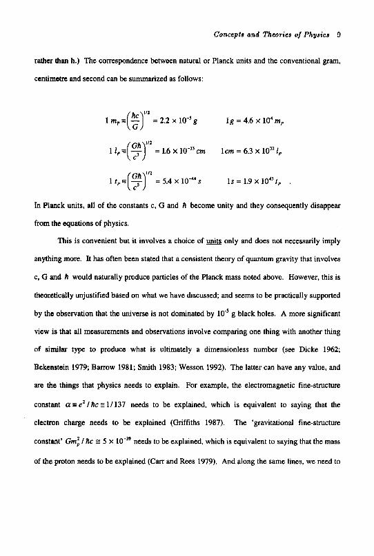
Concepts and Theories of Physics 9
rather than h.) The correspondence between natural or Planck units and the conventional gram,
centimetre and second can be summarized as follows:
1/2
1 I , %($) = 1.6 x cm lcm = 6.3 x lo” I ,
112
1 fp.(F) = 5.4 x 1 0 4 s I S = 1.9 x 1043t, .
In Planck units, all of the constants c, G and h become unity and they consequently disappear
from the equations of physics.
This is convenient but it involves a choice of units only and does not necessarily imply
anything more. It has often been stated that a consistent theory of quantum gravity that involves
c, G and A would naturally produce particles of the Planck mass noted above. However, this is
theoretically unjustified based on what we have discussed; and seems to be practically supported
by the observation that the universe is not dominated by l o 5 g black holes. A more significant
view is that all measurements and observations involve comparing one thing with another thing
of similar type to produce what is ultimately a dimensionless number (see Dicke 1962;
Bekenetein 1979; Barrow 1981; Smith 1983; Wesson 1992). The latter can have any value, and
are the things that physics needs to explain. For example, the electromagnetic fine-structure
constant a = e ’ / h c = 1/137 needs to be explained, which is equivalent to saying that the
electron charge needs to be explained (Griffiths 1987). The ‘gravitational fine-structure
constant’ Gmi / hc P 5 x needs to be explained, which is equivalent to saying that the mass
of the proton needs to be explained (Cam and Rees 1979). And along the same lines, we need to
10 Space, Time, Matter
explain the constant involved in the observed correlation between the spin angular momenta and
masses of astronomical objects, which is roughly GM2/Jc G 1/300 (Wesson 1983). In other
words, we get no more out of dimensional analysis and a choice of units than is already pnsent
in the underlying equations, and neither technique is a substitute for proper physics.
The physics of explaining the charge of the electron or the mass of a proton, referred to
above, probably lies in the future. However, some comments can be made now. As regards e, it
is an observed fact that a is energy or distance-dependent. Equivalently, e is not a fundamental
constant in the same class as c, h and G. The current explanation for this involves vacuum
polarization, which effectively screens the charge of one particle as experienced by another (see
Section 1.4). This mechanism is depressingly mechanical to some field theorists, and in
attributing an active role to the vacuum would have been anathema to Einstein. [There are also
alternative explanations for it, such as the influence of a scalar field, as discussed in Nodvik
(1985) and Chapter 5.1 However, the philosophy of trying to understand the electron charge,
rather than just accepting it as a given, has undoubted merit. The same applies to the masses of
the elementary particles, which however are unquantized and so present more of a challenge.
The main question is not whether we wish to explain charges and masses, but rather what is the
best approach.
In this regard, we note that both are geometrizable (Hoyle and Narlikar 1974; Wesson
1992). The rest mass of a particle m is the easiest to treat, since using G or h we can convert m
to a length:
h x, 3 - Gm c2 me
x =- or
Physically, the choice here would conventionally be described as one between gravitational or
atomic units, a ploy which has been used in several theories that deal with the nature of mass
Concepts and Theories of Physics 11
(see Wesson 1978 for a review). Mathematically, the choice is one of coordinates, provided we
absorb the constants and view mass as on the same footing as time and space (see Chapter 7).
The electric charge of a particle q is harder to treat, since it can only be geometrized by including
the gravitational constant via xq = (G/c4)”’q. This, together with the trite but irrefutable fact
that masses can carry charges but not the other way round, suggests that mass is more
fundamental than charge.
1.3 Gt neral Relativity
In the original form of this theory due to Einstein, space is regarded as a construct in
which only the relations between objects have meaning. The theory agrees with all observations
of gravitational phenomena, but the best books that deal with it are those which give a fair
treatment of the theory’s conceptual implications. Notably, those by Weinberg (1972). Misner,
Thome and Wheeler (1973), Rindler (1977) and Will (1993). We should also mention the book
by Jammer (1961) on concepts of mass; and the conference proceedings edited by Barbour and
Pfister (1995) on the idea due to Mach that mass locally depends on the distribution of matter
globally. The latter was of course a major motivation for Einstein, and while not incorporated
into standard general relativity is an idea that will reoccur in subsequent chapters.
The theory is built on 10 dimensionless potentials which are the independent elements in
a 4 x 4 metric tensor gd (a,p = 0-3). These define the square of the distance between 2 nearby
points in 4D via ds2 = g,dradrs. (Here a repeated index upstairs and downstairs is summed
over, and below we will use the metric tensor to raise and lower indices on other tensors.) The
coordinates xa are in a local limit identified as xo = ct, x’ = x, x2 = y, x3 = z using Cartesians.
However, because the theory employs tensors and therefore gives relations valid in any system
12 Space, Time, M a t t e r
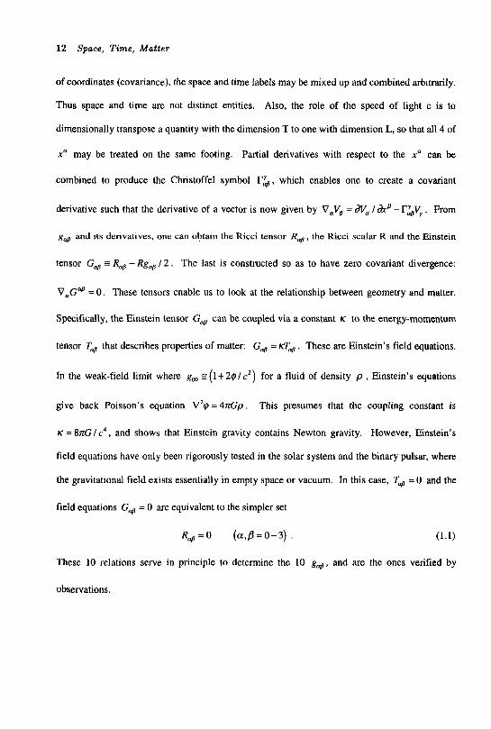
of coordinates (covariance), the space and time labels may be mixed up and combined arbitrarily.
Thus space and time are not distinct entities. Also, the role of the speed of light c is to
dimensionally transpose a quantity with the dimension T to one with dimension L, so that all 4 of
x a may be treated on the same footing. Partial derivatives with respect to the xu can be
combined to produce the Christoffel symbol r&, which enables one to create a covariant
derivative such that the derivative of a vector is now given by VaVa = dVa / - r&Vy . From
g, and its derivatives, one can obtain the Ricci tensor Raa , the Ricci scalar R and the Einstein
tensor G, = R, - Rg, / 2 . The last is constructed so as to have zero covariant divergence:
V,G@ = 0. These tensors enable us to look at the relationship between geometry and matter.
Specifically, the Einstein tensor G, can be coupled via a constant K to the energy-momentum
tensor Td that describes properties of matter: G, = fl, . These are Einstein’s field equations.
In the weak-field limit where g, s ( l + 2 # / c z ) for a fluid of density p , Einstein’s equations
give back Poisson’s equation V 2 # = 4 n C p . This presumes that the coupling constant is
K = 8nC / c4, and shows that Einstein gravity contains Newton gravity. However, Einstein’s
field equations have only been rigorously tested in the solar system and the binary pulsar, where
the gravitational field exists essentially in empty space or vacuum. In this case, T, = 0 and the
field equations G, = 0 are equivalent to the simpler set
R, = O ( 0 l , P = 0 - 3 ) . (1.1)
These 10 relations serve in principle to determine the 10 g,, and are the ones verified by
observations.
Concepts and Theories of Physics 13
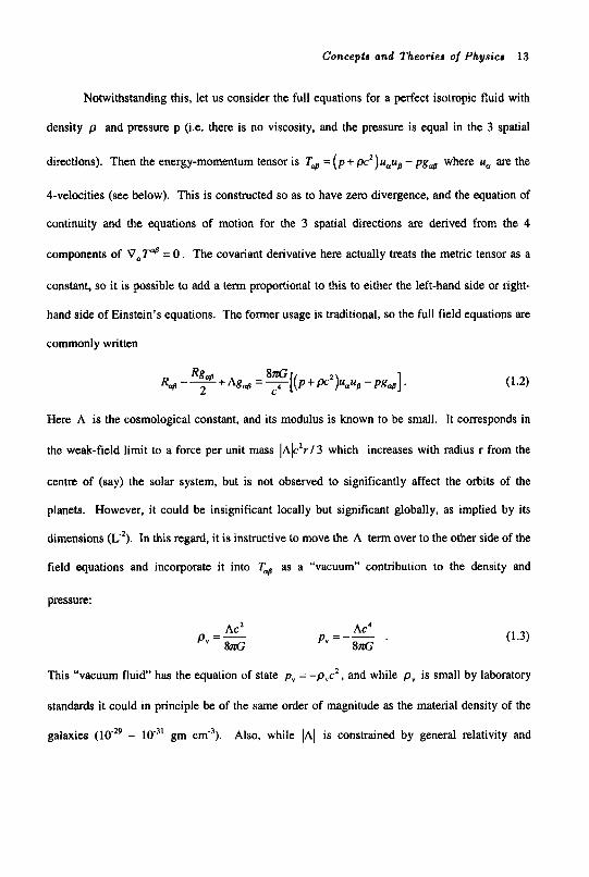
Notwithstanding this, let us consider the full equations for a perfect isotropic fluid with
density p and pressure p (i.e. there is no viscosity, and the pressure is equal in the 3 spatial
directions). Then the energy-momentum tensor is T+ = (p + pc2)u,ue - pg, where u, are the
4-velocities (see below). This is constructed so as to have zero divergence, and the equation of
continuity and the equations of motion for the 3 spatial directions are derived from the 4
components of V,T@ = 0 . The covariant derivative here actually treats the metric tensor as a
constant, so it is possible to add a term proportional to this to either the left-hand side or right-
hand side of Einstein’s equations. The former usage is traditional, so the full field equations are
commonly written
Here A is the cosmological constant, and its modulus is known to be small. It corresponds in
the weak-field limit to a force per unit mass IAlczr/3 which increases with radius r from the
centre of (say) the solar system, but is not observed to significantly affect the orbits of the
planets. However, it could be insignificant locally but significant globally, as implied by its
dimensions (L-’). In this regard, it is instructive to move the A term over to the other side of the
field equations and incorporate it into T, as a “vacuum” contribution to the density and
pressure:
Acz p =- ” 8 s
Ac4 8nG
p , = - - . (1.3)
This “vacuum fluid’’ has the equation of state p , = -pvc2, and while p, is small by laboratory
standards it could in principle be of the same order of magnitude as the material density of the
galaxies Also, while 1A1 is constrained by general relativity and - 10.’’ gm cm-’).
14 Space, Time, Matter
observations of the present universe, there are arguments concerning the stability of the vacuum
from quantum field theory which imply that it could have been larger in the early universe. But
A (and G,c) are true constants in the original version of general relativity, so models of quantum
vacuum transitions involve step-like phase changes (see e.g. Henriksen, Emslie and Wesson
1983). It should also be noted that while matter in the present universe has a pressure that is
positive or close to zero (“dust”), there is in principle no reason why in the early universe or
other exotic situations it cannot be taken negative. Indeed, any microscopic process which
causes the particles of a fluid to attract each other can in a macroscopic way be described by p <
0 (the vacuum treated classically is a simple example). In fact, it is clear that p and p in general
relativity are phenomenological, in the sense that they are labels for unexplained particle
processes. It is also clear that the prime function of G and c is to dimensionally transpose matter
labels such a s p and p so that they match the geometrical objects of the theory.
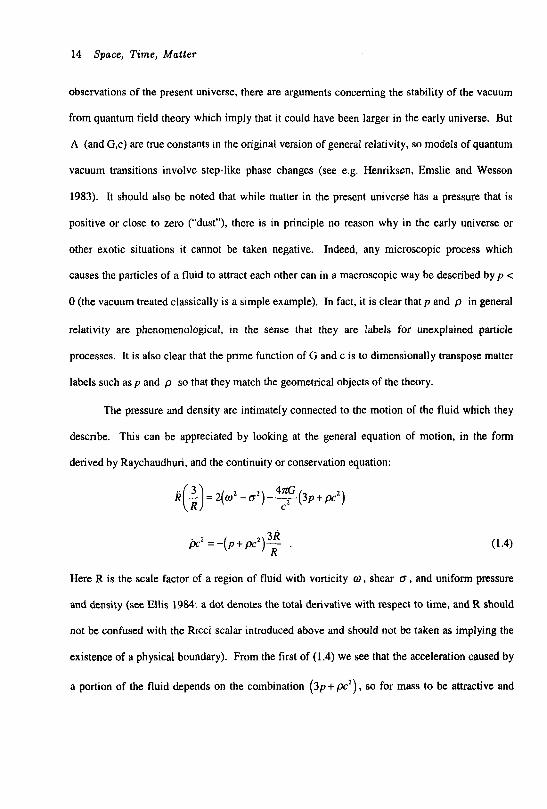
The pressure and density are intimately connected to the motion of the fluid which they
describe. This can be appreciated by looking at the general equation of motion, in the form
derived by Raychaudhuri, and the continuity or conservation equation:
4nc R - = 2 ( o ~ - o ~ ) - ~ ( 3 P + p c z ) (3 3k
jJcz =(p+pc*)- . R
Here R is the scale factor of a region of fluid with vorticity w , shear d , and uniform pressure
and density (see Ellis 1984: a dot denotes the total derivative with respect to time, and R should
not be confused with the Ricci scalar introduced above and should not be taken as implying the
existence of a physical boundary). From the first of (1.4) we see that the acceleration caused by
a portion of the fluid depends on the combination ( 3 p + pc’) , so for mass to be attractive and
Concepts and Theories of Ph$rsics 15
positive we need ( 3 p + p.’) > 0. From the second of (1.4), we see that the rate of change of
density depends on the combination (p + p.’), so for matter to be stable in some sense we need
( p + pc’) > 0 . These inequalities, sometimes called the energy conditions, should not however
be considered sacrosanct. Indeed, gravitational energy is a slippery concept in general relativity,
and there are several alternative definitions of “mass” (Hayward 1994). These go beyond the
traditional concepts of active gravitational mass as the agent which causes a gravitational field,
passive gravitational mass as the agent which feels it, and inertial mass as the agent which
measures energy content (Bonnor 1989). What the above shows is that in a fluid-dynamical
context, ( 3 p + p 2 ) is the gravitational energy density and ( p + p . ’ ) is the inertial energy
density.
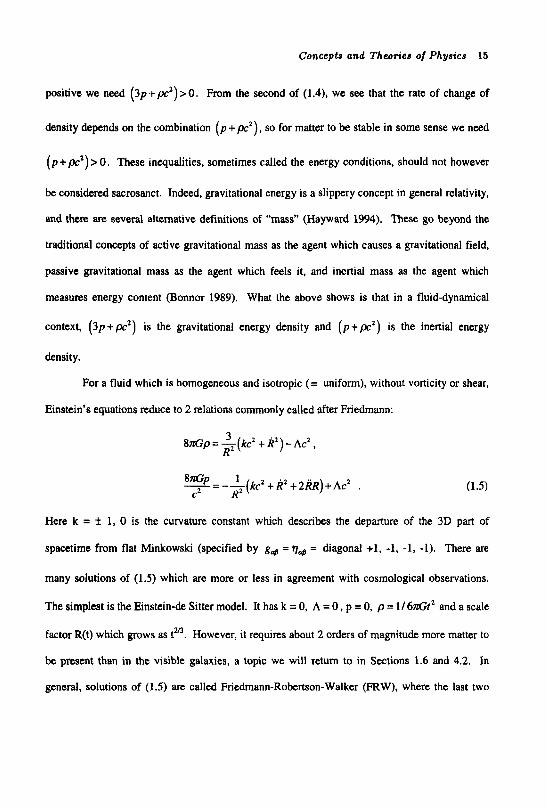
For a fluid which is homogeneous and isotropic (= uniform), without vorticity or shear,
Einstein’s equations reduce to 2 relations commonly called after Friedmann:
3 R’
8nGp = -(kz + h2) - Ac’,
8nGp 1 - = --( kc2 + k2 + 2kR) + Ac2 c’ RZ
Here k = f 1, 0 is the curvature constant which describes the departure of the 3D part of
spacetime from flat Minkowski (specified by gM = qM = diagonal +1, -1, -1, -1). There are
many solutions of (1.5) which are more or less in agreement with cosmological observations.
The simplest is the Einstein-de Sitter model. It has k = 0, A = 0 , p = 0, p = 1/61d;rz and a scale
factor R(t) which grows as t”. However, it requires about 2 orders of magnitude more matter to
be present than in the visible galaxies, a topic we will return to in Sections 1.6 and 4.2. In
general, solutions of (1.5) are called Friedmann-Robertson-Walker (FRW), where the last two
16 Space, Time, Matter
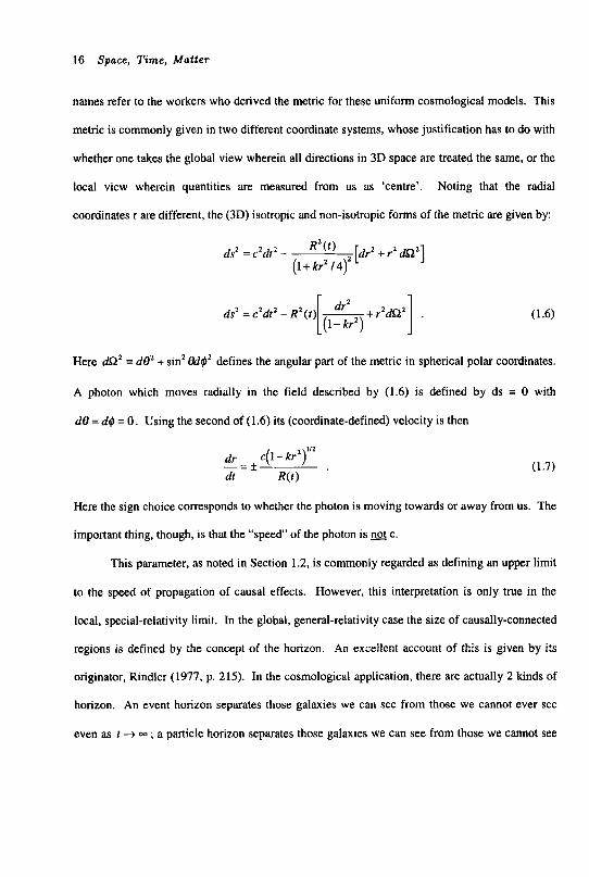
names refer to the workers who derived the metric for these uniform cosmological models. This
metric is commonly given in two different coordinate systems, whose justification has to do with
whether one takes the global view wherein all directions in 3D space are treated the same, or the
local view wherein quantities are measured from us as 'centre'.
coordinates rare different, the (3D) isotropic and non-isotropic forms of the metric are given by:
Noting that the radial
dsz = c2dt2 - R 2 ( t ) [dr2 + r2 dQ2] (1 + kr2 I 4 )
Here dQ2 = do2 +sinZ &ig2 defines the angular part of the metric in spherical polar coordinates.
A photon which moves radially in the field described by (1.6) is defined by ds = 0 with
d6 = d# = 0. Using the second of (1.6) its (coordinate-defined) velocity is then
Here the sign choice corresponds to whether the photon is moving towards or away from us. The
important thing, though, is that the "speed' of the photon is c.
This parameter, as noted in Section 1.2, is commonly regarded as defining an upper limit
to the speed of propagation of causal effects. However, this interpretation is only true in the
local, special-relativity limit. In the global, general-relativity case the size of causally-connected
regions is defined by the concept of the horizon. An excellent account of this is given by its
originator, Rindler (1977, p. 215). In the cosmological application, there are actually 2 kinds of
horizon. An event horizon separates those galaxies we can see from those we cannot ever see
even as t + m ; a particle horizon separates those galaxies we can see from those we cannot see
Concepts and Theories of Physics 17
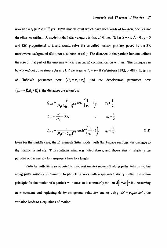
now at t = bJ (e 2 x 10" yr). FRW models exist which have both kinds of horizon, one but not
the other, or neither. A model in the latter category is that of Milne. (It has k = -1, A = 0, p = 0
and R(t) proportional to t, and would solve the so-called horizon problem posed by the 3K
microwave background did it not also have p = 0 .) The distance to the particle horizon defines
the size of that part of the universe which is in causal communication with us. The distance can
be worked out quite simply for any k if we assume A = p = 0 (Weinberg 1972, p. 489). In terms
of Hubble's parameter now (H, I I&/&, ) and the deceleration parameter now
(qo = -&J$ / e) , the distances are given by:
Even for the middle case, the Einstein-de Sitter model with flat 3-space sections, the distance to
the horizon is not cbJ. This confirms what was noted above, and shows that in relativity the
purpose of c is merely to transpose a time to a length.
Particles with finite as opposed to zero rest masses move not along paths with ds = 0 but
along paths with s a minimum. In particle physics with a special-relativity metric, the action
principle for the motion of a particle with mass m is commonly written S[jmds] = 0 . Assuming
m = constant and replacing ds by its general relativity analog using ds2 = g,dr"dxa, the
variation leads to 4 equations of motion:
18 Space, Time, Matter
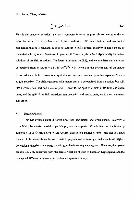
dur ds
-++&uaufl = o .
This is the geodesic equation, and its 4 components serve in
velocities ur I dry l d s as functions of the coordinates. We
principle to determine
note that. in addition
(1.9)
the 4-
to the
assumDtion that m is constant, m does not appear in (1.9): general relativity is not a theory of
forces but a theory of accelerations. In practice, (1.9) can only be solved algebraically for certain
solutions of the field equations. The latter in vacuum are (l . l) , and we note here that these can
be obtained from an action via 6 [ ~ R ( - g ) ” * d ‘ x ] = O . Here g is the determinant of the metric
tensor, which with the conventional split of spacetime into time and space has signature (+ - - -)
so g is negative. The field equations with matter can also be obtained from an action, but split
into a geometrical part and a matter part. However, the split of a metric into time and space
parts, and the split of the field equations into geometric and matter parts, are to a certain extent
subjective.
1.4 Particle Phvsics
This has evolved along different lines than gravitation, and while general relativity is
monolithic, the standard model of particle physics is composite. Of relevance are the books by
Ramond (1981), Griffiths (1987), and Collins, Martin and Squires (1989). The last is a good
review of the connections between particle physics and cosmology, and also treats higher-
dimensional theories of the types we will examine in subsequent sections. However, the present
section is mainly concerned with standard 4D particle physics as based on Lagrangians, and the
conceptual differences between gravitation and quantum theory.
Concepts and Theories of Physics 19
The material is ordered by complexity: we consider the equations of Maxwell,
Schrodinger, Klein-Gordon, Dirac, Proca and Yang-Mills; and then proceed to quantum
chromodynamics and the standard model (including Glashow-Salam-Weinberg theory). As
before, there is an emphasis on fundamental constants and the number of parameters required to
make theory compatible with observation.
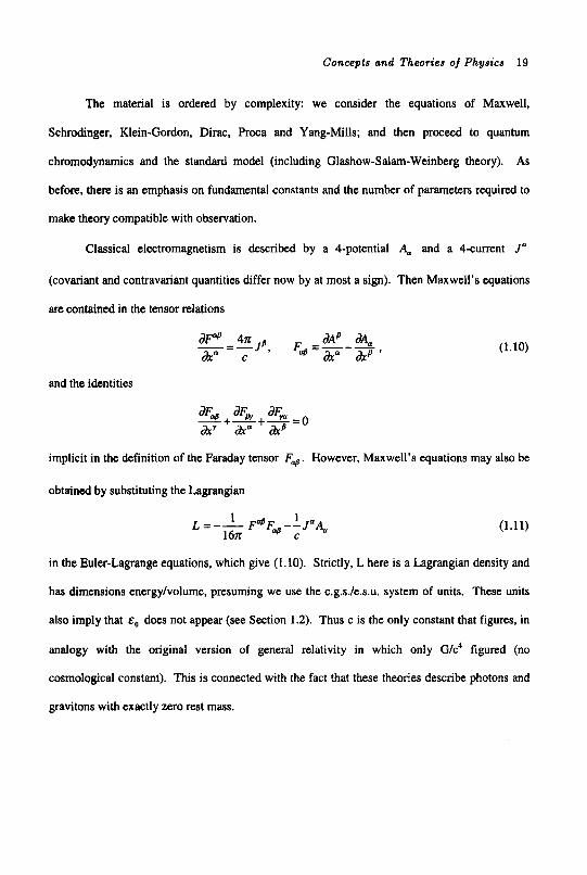
Classical electromagnetism is described by a 4-potential Aa and a 4-current J”
(covariant and contravariant quantities differ now by at most a sign). Then Maxwell’s equations
are contained in the tensor relations
and the identities
(1.10)
implicit in the definition of the Faraday tensor F, . However, Maxwell’s equations may also be
obtained by substituting the Lagrangian
(1.11)
in the Euler-Lagrange equations, which give (1.10). Strictly, L here is a Lagrangian density and
has dimensions energy/volume, presuming we use the c.g.s./e.s.u. system of units. These units
also imply that E, does not appear (see Section 1.2). Thus c is the only constant that figures, in
analogy with the original version of general relativity in which only G/c4 figured (no
cosmological constant). This is connected with the fact that these theories describe photons and
gravitons with exactly zero rest mass.
20 Space, Time, Matter
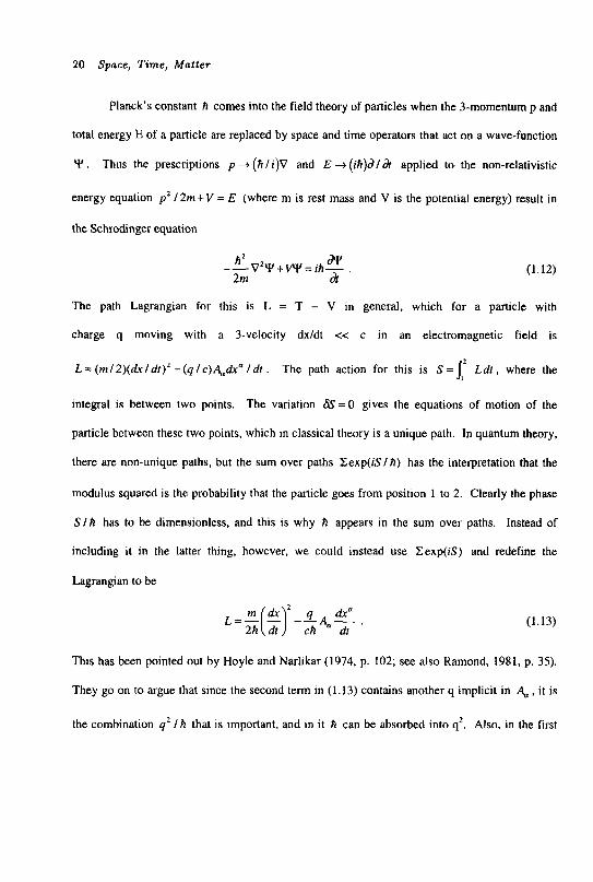
Planck's constant h comes into the field theory of particles when the 3-momentum p and
total energy E of a particle are replaced by space and time operators that act on a wave-function
Y . Thus the prescriptions p 4 ( h / i)V and E -+ ( ih)dl b applied to the non-relativistic
energy equation p z /2m+V = E (where m is rest mass and V is the potential energy) result in
the Schrodinger equation
(1.12)
The path Lagrangian for this is L = T - V in general, which for a particle with
charge q moving with a 3-velocity dxldt <i c in an electromagnetic field is
L = ( m 1 2 ) ( d x l d t ) Z - ( q l c ) ~ d x " I d ? . The path action for this is S = P L d t , where the
integral is between two points. The variation &S = 0 gives the equations of motion of the
particle between these two points, which in classical theory is a unique path. In quantum theory,
there are non-unique paths, but the sum over paths Cexp(iSlh) has the interpretation that the
modulus squared is the probability that the particle goes from position 1 to 2. Clearly the phase
S l h has to be dimensionless, and this is why A appears in the sum over paths. Instead of
including it in the latter thing, however, we could instead use Zexp(iS) and redefine the
Lagrangian to be
(1.13)
This has been pointed out by Hoyle and Narlikar (1974, p. 102; see also Ramond, 1981, p. 35).
They go on to argue that since the second term in (1.13) contains another q implicit in 4, it is
the combination q2 l h that is important, and in it h can be absorbed into q2. Also, in the first
Concepts and Theories of Physics 21
term in (1.13) it is the combination m / A that is important, and in it A can be absorbed into m.
Thus the Lagrangian reduces back to the f o n given before.
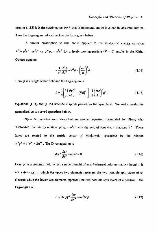
A similar prescription to that above applied to the relativistic energy equation
EZ - p2cz = m2c4 or pap , = mZcZ for a freely-moving particle (V = 0) results in the Klein-
Gordon equation
Here # is a single scalar field and the Lagrangian is
(1.14)
(1.15)
Equations (1.14) and (1.15) describe a spin-0 particle in flat spacetime. We will consider the
generalization to curved spacetime below.
Spin-1/2 particles were described in another equation formulated by Dirac, who
'factorized' the energy relation papu = m2c2 with the help of four 4 x 4 matrices y" . These
latter are related to the metric tensor of Minkowski spacetime by the relation
y a y B + y B y " = 29@, The Dirac equation is
iAy"-- m c y = O . (1.16) dx"
Here y is a bi-spinor field, which can be thought of as a 4-element column matrix (though it is
not a 4-vector) in which the upper two elements represent the two possible spin states of an
electron while the lower two elements represent the two possible spin states of a positron. The
Lagrangian is
dl L = ihcw" - - mc'ijiy . axa (1.17)

22 Space, Time, Matter
Here v is the adjoint spinor defined by r J = y t y o , where y' is the usual Hermitian or
transpose conjugate obtained by transposing y from a column to a row matrix and complex-
conjugating its elements. The Lagrangian (1.17) is for a free particle. It is invariant under the
global gauge or phase transformation ty +eiey (where 8 is any real number), because
v + e-iav and the exponentials cancel out in the combination i@y . But it is not invariant under
the local gauge transformation ty + e"(')W which depends on location in spacetime. If the
principle of local gauge invariance is desired, it is necessary to replace (1.17) by
(1.18) dty dx"
L = ihc@'" - - rnc'vyf - q@4,uAa.
Here A, is a potential which we identify with electromagnetism and which changes under local
gauge transformations according to A, --f A, +dA/dx* where A(.") is a scalar function. In
fact, we can say that the requirement of local gauge invariance for the Dirac Lagrangian (1.18)
obliges the introduction of the field A, typical of electromagnetism.
Actually the Lagrangian (1.18) should be even further extended by including a 'free' term
for the gauge field. In this regard, the transformation Aa -+ 4 t ad / &a leaves FM
unchanged, but not a term like AaA,. The appropriate term to add to (1.18) is therefore
(-1/16n)F@F,, so the full Dirac Lagrangian is
(1.19)
If we define a current density J" I cq(vyy"ty) , the last two terms give back Maxwell's
Lagrangian (1.1 1). The Lagrange density (1.19) describes electrons or positrons interacting with
an electromagnetic field consisting of massless photons. However, a term like the one we just
Concepts and Theories of Physics 23
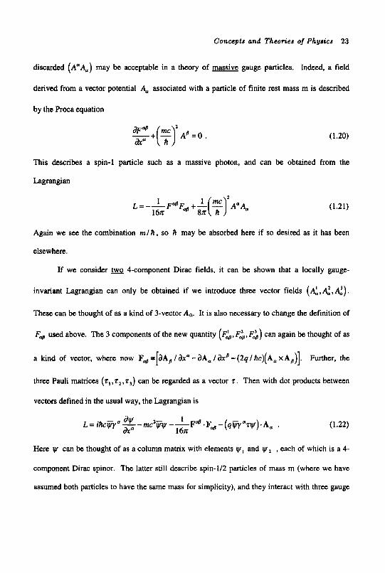
discarded (Aa&) may be acceptable in a theory of massive gauge particles. Indeed, a field
derived from a vector potential & associated with a particle of finite rest mass m is described
by the Proca equation
(1.20)
This describes a spin-1 particle such as a massive photon, and can be obtained from the
Lagrangian
(1.21)
Again we see the combination m / A , so A may be absorbed here if so desired as it has been
elsewhere.
If we consider &Q 4-component Dirac fields, it can be shown that a locally gauge-
invariant Lagrangian can only be obtained if we introduce three vector fields (&,g,&).
These can be thought of as a kind of 3-vector A,. It is also necessary to change the definition of
F, used above. The 3 components of the new quantity (Fb,,F$, F;) can again be thought of as
a kind of vector, where now F, =[aA, /axa -aAa / a x @ -(2q/Ac)(A, x A,)]. Further, the
three Pauli matrices (zI,zz,zj) can be regarded as a vector z. Then with dot products between
vectors defined in the usual way, the Lagrangian is
(1.22)
Here y can be thought of as a column matrix with elements w I and w2 , each of which is a 4-
component Dirac spinor. The latter still describe spin-1/2 particles of mass m (where we have
assumed both particles to have the same mass for simplicity), and they interact with three gauge
24 Space, Time, Matter
fields 4,&,& which by gauge invariance must be massless. The lund of gauge invariance
obeyed by (1.22) is actually more complex than that involving global and local phase
transformations with eis considered above. There I was a single spinor, whereas here y is a
2-spinor column matrix. This leads us to consider a 2 x 2 matrix which we take to be unitary
(U'U = 1). In fact the first two terms in (1.22) are invariant under the global transformation
ty -+ Uw , because q+ ijiU+ so the combination Fw is invariant. Just as any complex number
of modulus 1 can be written as eis with 8 real, any unitary matrix can be written U = el" with
H Hermitian (H' = H) . Since H i s a 2 x 2 matrix it involves 4 real numbers, say 8 and al, a2. a3
which can be regarded as the components of a 3-vector a. As before, let z be the 3-vector whose
components are three 2 x 2 Pauli matrices, and let 1 stand for the 2 x 2 unit matrix. Then without
loss of generality we can write H = 81 + v a , so U = eieei"". The first factor here is the old
phase transformation. The second is a 2 x 2 unitary matrix which is special in that the
determinant is actually 1. Thus w + e'r'ay is a global special-unitary 2-parameter, or SU(2),
transformation. It should be recalled that this global invariance only involves the first two terms
of the Lagrangian (1.22), which resemble the Lagrangian (1.17) of Dirac. The passage to local
invariance along lines similar to those considered above leads to the other terms in the
Lagrangian (1.22) and was made by Yang and Mills.
The full Yang-Mills Lagrangian (1.22) is invariant under local SU(2) gauge
transformations, and leads to field equations that were originally supposed to describe two equal-
mass spin-112 particles interacting with three massless spin-1 (vector) particles. In this form the
theory is somewhat unrealistic, but still useful. For example, if we drop the first two terms in
(1.22) we obtain a Lagrangian for the three gauge fields alone which leads to an interesting
classical-type field theory that resembles Maxwell electrodynamics. This correspondence
Concepts and Theories of Physics 25
becomes clear if like before we define currents J" I c q ( ~ ' ? y ) , whereby the last two terms in
(1.22) give a gauge-field Lagrangian
(1.23)
This closely resembles the Maxwell Lagrangian (1.11). But of course (1.23) gives rise to a
considerably more complicated theory, solutions of which have been reviewed by Actor (1979).
Some of these represent magnetic monopoles, which have not been observed. Some represent
instantons and merons, which are hypothetical particles that tunnel between topologically distinct
vacuum regions. For example,
Vilenkin (1982) has suggested that a certain type of instanton tunneling to de Sitter space from
nothing can give birth to an inflationary universe. However, it is doubtful if the kinds of
particles predicted by pure SU(2) Yang-Mills theory will ever have practical applications. The
real importance of this theory is that it showed it was feasible to use a symmetry group involving
non-commuting 2 x 2 matrices to construct a non-Abelian gauge theory. This idea led to more
successful theories, notably one for the strong interaction based on SU(3) colour symmetry.
[email protected] 1 - -J".A 1 16n @ c
Tunneling can in principle be important cosmologically.
Quantum chromodynamics (QCD) is described by 3 coloured Dirac spinors that can be
denoted yd, wbluc, w, and 8 gauge fields given by a kind of 8-vector A,. Each of
w,, l y b , w, is a 4-component Dirac spinor, and it is convenient to regard them as the elements
of a column matrix ly. This describes the colour states of a massive spin-112 quark. The 8
components of A, are associated with the 8 Gell-Mann matrices (al-*), which are the SU(3)
equivalents of the Pauli matrices of SU(2), and describe massless spin-1 gluons. The Lagrangian
for QCD can be constructed by adding together 3 Dirac Lagrangians like (1.17) above (one for
each colour), insisting on local SU(3) gauge invariance (which brings in the 8 gauge fields), and
26 Space, Time, Matter
adding in a free gauge-field term (using Fns as defined above for the original Yang-Mills
theory). The complete Lagrangian is
(1.24)
This resembles (1.22) above. However, the electric charge of a quark needs to be a fraction of e
in order to account for the common hadrons as quark composites. And particle physics is best
described by 6 quarks with different flavours (d, u, s, c, b, t) and different masses m. This means
we really need 6 versions of (1.24) with different masses. A gluon does not carry electric charge,
but it does carry colour charge. This is unlike its analogue the photon in electrodynamics,
allowing bound gluon states (glueballs) and making chromodynamics generally quite
complicated.
We do not need to go into the intricacies of QCD, especially since good reviews are
available (Ramond 1981; Llewellyn Smith 1983; Griffiths 1987; Collins, Martin and Squires
1989). But a couple of points related to charges and masses are relevant to our discussion. In
the case of electrons interacting via photons, the Dirac Lagrangian and the fact that
a z e2 lhc E 1/ 137 is small allows perturbation analysis to be used to produce very accurate
models. Indeed, quantum electrodynamics (QED) gives predictions that are in excellent
agreement with experiment. However, the coupling parameter whose asymptotic value is the
traditional fine-structure constant is actually energy or distance dependent. As mentioned in
Section 1.2, this is commonly ascribed to vacuum polarization. Thus, a positive charge (say)
surrounded by virtual electrons and positrons tends to attract the former and repel the latter.
(Virtual particles do not obey Heisenberg's uncertainty relation and in modern quantum field
theory the vacuum is regarded as full of them.) There is therefore a screening process, which
means that the effective value of the embedded charge (and a) increases as the distance
Concepts and Theories of Physics 27
decreases. In analogy with QED, there is a similar process in QCD, but due to the different
nature of the interaction the coupling parameter decreases as the distance decreases. This is the
origin of asymptotic freedom, whose converse is that quarks in (say) a proton feel a strong
restoring force if they move outwards and are in fact confined. In addition to the variable nature
of coupling ‘constants’ and charges, the masses in QCD are also not what they appear to be. The
m which appears in a Lagrangian like (1.24) is not really a given parameter, but is believed to
arise from the spontaneous symmetry breaking which exists when a symmetry of the Lagrangian
is not shared by the vacuum. Thus a manifestly symmetric Lagrangian with massless gauge-field
particles can be rewritten in a less symmetric form by redefining the fields in terms of
fluctuations about a particular ground state of the vacuum. This results in the gauge-field
particles becoming massive and in the appearance of a massive scalar field or Higgs particle. In
QCD. the quarks are initially taken to be massless, but if they have Yukawa-type couplings to the
Higgs particle then they acquire masses. The Higgs mechanism in QCD, however, is really
imported from the theory of the weak interaction, and has been mentioned here to underscore
that the masses of the quarks are not really fundamental parameters.
The theory of the weak interaction was originally developed by Fermi as a way of
accounting for beta decay, but is today mainly associated with Glashow, Weinberg and Salam
who showed that it was possible to unify the weak and electromagnetic interactions (for reviews
see Salam 1980 and Weinberg 1980). As it is formulated today, the theory of the weak
interaction involves mediation by 3 very massive intermediate vector (spin-1) bosons, two of
which (W*) are electrically charged and one of which (p) is neutral. These can be combined
with the photon of electromagnetism via the symmetry group SU(2) 0 U(I), which is however
spontaneously broken by the mechanism outlined in the preceding paragraph. Actually, the
28 Space, Tame, Matter
massive Zo and the massless photon are combinations of states that depend on a weak mixing
angle 8, whose value is difficult to calculate from theory but is 8, 5 29' from experiment. The
theory of the weak interaction, like QED and QCD, involves a coupling parameter which is not
constant.
What we have been discussing in the latter part of this section are parts of the standard
model of particle physics, which symbolically unifies the electromagnetic, weak and strong
interactions via the symmetry group U(1) BSU(2) 8 SU(3). An appealing feature of this
theory is that with increasing energy the electromagnetic coupling increases while the weak and
strong couplings decrease, suggesting that they come together at some unifying energy. This,
however, is not known: it is probably of order 10l6 GeV, but could be as large as the Planck mass
of order 10'' GeV (see Weinberg 1983; Llewellyn Smith 1983; Ellis 1983; Kibble 1983;
Griffiths 1987, p. 77; Collins, Martin and Squires 1989, p. 159). Also, there are uncertainties in
the theory, notably to do with the QCD sector where the numbers of colors and flavors are
conventionally taken as 3 and 6 respectively but could be different. This means that while in the
conventional model there are 6 quark masses and 6 lepton masses, there could be more. In fact,
if we include couplings and other things, there are. at least 20 parameters in the theory (Ellis
1983). One might hope to reduce this by using a simple unifying group for U(1), SU(2) and
SU(3). but the minimal example of SU(5) does not actually help much in this regard. And then
there is the perennial question: What about gravity?
1.5 Kaluza-Klein Theory
The idea that the world may have more than 4 dimensions is due to Kaluza (1921), who
with a brilliant insight realized that a 5D manifold could be used to unify Einstein's theory of
Concepts and Theories of Physics 29
general relativity (Section 1.3) with Maxwell’s theory of electromagnetism (Section 1.4). After
some delay, Einstein endorsed the idea, but a major impetus was provided by Klein (1926). He
made the connection to quantum theory by assuming that the extra dimension was
microscopically small, with a size in fact connected via Planck’s constant h to the magnitude of
the electron charge e (Section 1.2). Despite its elegance, though, this version of Kaluza-KTein
theory was largely eclipsed by the explosive development first of wave mechanics and then of
quantum field theory. However, the development of particle physics led eventually to a
resurgence of interest in higher-dimensional field theories as a means of unifying the long-range
and short-range interactions of physics. Thus did Kaluza-Klein 5D theory lay the foundation for
modem developments such as 11D supergravity and 1OD superstrings (Section 1.6). In fact,
there is some ambiguity in the scope of the phrase “Kaluza-Klein theory”. We will mainly use it
to refer to a 5D field theory, but even in that context there are several versions of it. The
literature is consequently enormous, but we can mention the conference proceedings edited by
De Sabbata and Schmutzer (1983), Lee (1984) and Appelquist, Chodos and Freund (1987). A
recent comprehensive review of all versions of Kaluza-Klein theory is the article by Overduin
and Wcsson (1997a). The latter includes a short account of what is referred to by different
workers as non-compactified, induced-matter or space-time-matter theory. Since this is the
subject of the following chapters, the present section will be restricted to a summary of the main
features of traditional Kaluza-Klein theory.
This theory is essentially general relativity in 5D, but constrained by two conditions.
Physically, both have the motivation of explaining why we perceive the 4 dimensions of
spacetime and (apparently) do not see the fifth dimension. Mathematically, they are somewhat
different, however. (a) The so-called ‘cylinder’ condition was introduced by Kaluza, and
30 Space, Time, Matter
consists in setting all partial derivatives with respect to the fifth coordinate to zero. It is an
extremely strong constraint that has to be applied at the outset of calculation. Its main virtue is
that it reduces the algebraic complexity of the theory to a manageable level. (b) The condition of
compactification was introduced by Klein, and consists in the assumption that the fifth
dimension is not only small in size but has a closed topology (i.e. a circle if we are only
considering one extra dimension). It is a constraint that may be applied retroactively to a
solution. Its main virtue is that it introduces periodicity and allows one to use Fourier and other
decompositions of the theory.
There are now 15 dimensionless potentials, which are the independent elements in a
symmetric 5 x 5 metric tensor gAB (A,B = 0-4: compare section 1.3). The first 4 coordinates are
those of spacetime, while the extra one x4 = 1 (say) is sometimes referred to as the “internal”
coordinate in applications to particle physics. In perfect analogy with general relativity, one can
form a 5D Ricci tensor RAB, a 5D Ricci scalar R and a 5D Einstein tensor GAB = RAB - RgA&.
The field equations would logically be expected to be G,, = kTAB with some appropriate
coupling constant k and a 5D energy-momentum tensor. But the latter is unknown, so from the
time of Kaluza and Klein onward much work has been done with the ‘vacuum’ or ‘empty’ form
of the field equations GAB = 0. Equivalently, the defining equations are
R,, = 0 ( A , B = 0 - 4 ) . (1.25)
These 15 relations serve to determine the 15 gAB, at least in principle.
In practice, this is impossible without some starting assumption about gAB. This is
usually connected with the physical situation being investigated. In gravitational problems, an
assumption about g,, = g,,(xc) is commonly called a choice of coordinates, while in particle
physics it is commonly called a choice of gauge. We will meet numerous concrete examples
Concepts and Theories of P h y ~ i c s 31
later, where given the functional form of g,,(xc) we will calculate the 5D analogs of the
Christoffel symbols r:B which then give the components of RAB (Chapters 2-4). Kaluza was
interested in electromagnetism, and realized that hB can be expressed in a form that involves the
4-potential 4 that figures in Maxwell's theory. He adopted the cylinder condition noted above,
but also put &24 = constant. We will do a general analysis of the electromagnetic problem later
(Chapter 5) , but here we look at an intermediate case where g,, = g,,(x"), g, = - @'(x").
This illustrates well the scope of Kaluza-Klein theory, and has been worked on by many people.
including Jordan (1947, 1955). Bergmann (1948), Thiry (1948), Lessner (1982), and Liu and
Wesson (1997). The coordinates or gauge are chosen so as to write the 5D metric tensor in the
form
where K is a coupling constant. Then the field equations (1.25) reduce to
(1.26)
(1.27)
Here G, and F, are the usual 4D Einstein and Faraday tensors (see sections 1.3 and 1.4
respectively), and T, is the energy-momentum tensor for an electromagnetic field given by
Tas =(gOBF,Frs 14- FayFBy)/2. Also O= g@V,V, is the wave operator, and the summation
convention is in effect. Therefore we recognize the middle member of (1.27) as the 4 equations
3 2 . Space, Time, Matter
of electromagnetism modified by a function, which by the last member of (1.27) can be thought
of as depending on a wave-like scalar field. The first member of (1.27) gives back the 10
Einstein equations of 4D general relativity, but with a right-hand side which in some sense
represents energy and momentum that are effectively derived from the fifth dimension. In short,
Kaluza-Klein theory is in general a unified account of gravity, electromagnetism and a scalar
field.
Kaluza’s case g, = - @ = - 1 together with the identification K = (16rrG / c4)”* makes
(1.27) read
V“F@ = O . (1.28)
These are of course the straight Einstein and Maxwell equations in 4D, but derived from vacuum
in 5D, a consequence which is sometimes referred to as the Kaluza-Klein “miracle”. However,
these relations involve by (1.27) the choice of electromagnetic gauge F@F@ = O and have no
contribution from the scalar field. The latter could well be important, particularly in application
to particle physics. In the language of that subject, the field equations (1.25) of Kaluza-Klein
theory describe a spin-2 graviton, a spin-1 photon and a spin-0 boson which is thought to be
connected with how particles acquire mass. The field equations can also be derived from a 5D
action 6 R(-g)”’d’x]= 0, in a way analogous to what happens in 4D Einstein theory. [I It is also possible to put Kaluza-Klein theory into formal correspondence with other 4D
theories, notably the Brans-Dicke scalar-tensor theory (see Overduin and Wesson 1997a). This
theory is sometimes cast in a form where the scalar field is effectively disguised by putting the
functional dependence into G, the gravitational ‘constant’. In this regard it belongs to a class of
Concepts and Theories of Physics 33
4D theories, which includes ones by Dirac, Hoyle and Narlikar and Canuto et al., where the
constants are allowed to vary with cosmic time (see Wesson 1978 and Barbour and Pfister 1995
for reviews). However, it should be stated with strength that Kaluza-Klein theory is essentially
5D, and trying to cast it into 4D form is technically awkward. It should also be noted that the
reasons for treating 4D fundamental constants in this way are conceptually obscure.
1.6 Supergravity and Superstrings
These are based on the idea of supersymmetry, wherein each boson (integral spin) is
matched with a fermion (half integral spin). Thus the particle which is presumed to mediate
classical gravity (the graviton) has a partner (the gravitino). This kind of symmetry is natural,
insofar as particle physics needs to account for both bosonic and fermionic matter fields. But it
is also attractive because it leads to a cancellation of the enonnous zero-point fields which
otherwise exist but whose energy density is not manifested in the curvature of space (this is
related to the so-called cosmological constant problem, which is discussed elsewhere). The
literature on supergravity and superstrings is diverse, but we can mention the review articles by
Witten (1981) and Duff (1996); and the books by West (1986) and Green, Schwan and Witten
(1987). The status of the electromagnetic zero-point field has been discussed by Wesson (1991).
There is an obvious connection between 5D Kaluza-Klein theory, 11D supergravity and 1OD
superstrings. But while the former is more-or-less worked out, the latter are still in a state of
development with an uncertain prognosis where it comes to their relevance to the real world. For
this reason, and also because supersymmetry lies outside the scope of the rest of this work, we
will content ourselves with a short history.
34 Space, Time, Matter
Supersymmetric gravity or supergravity began life as a 4D theory in 1976 but quickly
It was particularly made the jump to higher dimensions (“Kaluza-Klein supergravity”).
successful in 1 ID, for three principal reasons. First, Nahm showed that 11 was the maximum
number of dimensions consistent with a single graviton (and an upper limit of two on particle
spin). This was followed by Witten’s proof that 11 was also the minimum number of dimensions
required for a Kaluza-Klein theory to unify all the forces in the standard model of particle
physics (i.e. to contain the gauge groups of the strong SU(3) and electroweak
SU(2) 8 U(1) interactions). The combination of supersymmetry with Kaluza-Klein theory thus
appeared to uniquely fix the dimensionality of the world. Second, whereas in lower dimensions
one had to choose between several possible configurations for the matter fields, Cremmer et al.
demonstrated in 1978 that in 11D there is a single choice consistent with the requirements of
supersymmetry (in particular, that there be equal numbers of Bose and Fermi degrees of
freedom). In other words, while a higher-dimensional energy-momentum tensor was still
required, its form at least appeared somewhat natural. Third, Freund and Rubin showed in 1980
that compactification of the 11D model could occur in only two ways: to 7 or 4 compact
dimensions, leaving 4 (or 7, respectively) macroscopic ones. Not only did 11D spacetime appear
to be specially favored for unification, but it also split perfectly to produce the observed 4D
world. (The other possibility, of a macroscopic 7D world, could however not be ruled out, and
in fact at least one such model was constructed as well.) Buoyed by these three successes, 11D
supergravity appeared set by the mid-1980s as a leading candidate for the hoped-for “theory of
everything”.
Unfortunately, certain difficulties have dampened this initial enthusiasm. For example,
the compact manifolds originally envisioned by Witten (those containing the standard model)
Concepts and Theories of Physics 35
turn out not to generate quarks or leptons, and to be incompatible with supenymmetry. Their
most successful replacements are the 7-sphere and the “squashed” 7-sphere, described
respectively by the symmetry groups SO(8) and SO(5) Q SU(2). But these groups do not
contain the minimum symmetry requirements of the standard model [SU(3) C3 SU(2) @ U(1)].
This is commonly rectified by adding matter-related fields, the “composite gauge fields”, to the
11D Lagrangian. Another problem is that it is very difficult to build chirality (necessary for a
realistic fermion model) into an 1 ID theory. A variety of remedies have been proposed for this,
including the common one of adding even more gauge fields, but none has been universally
accepted. It should also be mentioned that supergravity theory is marred by a large cosmological
constant in 4D, which is difficult to remove even by fine-tuning. Finally, quantization of the
theory inevitably leads to anomalies.
Some of these difficulties can be eased by descending to 10 dimensions: chirality is easier
to obtain, and many of the anomalies disappear. However, the introduction of chiral fermions
leads to new kinds of anomalies. And the primary benefit of the 11D theory - its uniqueness - is
lost: 1OD is not specially favored, and the theory does not break down naturally into 4
macroscopic and 6 compact dimensions. (One can still find solutions in which this happens, but
there is no reason why they should be preferred.) In fact, most 10D supergravity models not
only require ad hoc higher-dimensional matter fields to ensure proper compactification, but
entirely ignore gauge fields arising from the Kaluza-Klein mechanism (i.e. from symmetries of
the compact manifold). A theory which requires all gauge fields to be effectively put in by hand
can hardly be considered natural.
A breakthrough in solving the uniqueness and anomaly problems of 1OD theory occurmi
when Green and Schwan and Gross et al. showed that there were 2 (and only 2) 1OD
36 Space, Time, Matter
supergravity models in which all anomalies could be made to vanish: those based on the groups
SO(32) and E, 8 EB , respectively. Once again, extra terms (known as Chapline-Manton terms)
had to be added to the higher-dimensional Lagrangian. This time, however, the addition was not
completely arbitrary; the extra terms were those which would appear anyway if the theory were a
low-energy approximation to certain kinds of supersymmetric string theory.
Supersymmetric generalizations of strings, or superstrings, are far from being understood.
However, they have some remarkable virtues. For example, they retain the appeal of strings,
wherein a point particle is replaced by an extended structure, which opens up the possibility of
an anomaly-free approach to quantum gravity. (They do this while avoiding the generic
prediction of tachyons, which plagued the old string theories.) Also, it is possible to make
connections between certain superstring states and extreme black holes. (This may help resolve
the problem of what happens to the information swallowed by classical singularities, which has
been long standing in general relativity.) It is true that, for a while, there was thought to be
something of a uniqueness problem for LOD superstrings, in that the groups SO(32) and E8 8 EB
admit five different string theories between them. But this difficulty was addressed by Witten,
who showed that it is possible to view these five theories as aspects of a single underlying
theory, now known as M-theory (for “Membrane”). The low-energy limit of this new theory,
furthermore, turns out to be 11D supergravity. So it appears that the preferred dimensionality of
spacetime may after all be 11, at least in regard to higher-dimensional theories which are
compactified.
Supersymmetric particles such as gravitinos and neutralinos, if they exist, could provide
the dark or hidden matter necessary to explain the dynamics of galaxies and bring cosmological
observations into line with the simplest 4D cosmological models (see Section 1.3). However,
Concepts and Theories of Physics 37
such 'dark' matter is probably not completely dark, because the particles concerned are unstable
to decay in realistic (non-minimal) supersymmetric theories, and will contribute photons to the
intergalactic radiation field. Observations of the latter can be used to constrain supersymmetric
weakly interacting massive particles (WIMPS). Thus gravitinos and neutralinos are viable dark-
matter candidates if they have decay lifetimes greater than of order 10" yr and lo9 yr
respectively (Overduin and Wesson 1997b). In this regard, they are favored over non-
supersymmetric candidates such as massive neutrinos, axions and a possible decaying vacuum
(Oveduin and Wesson 1997c, 1992). There are other candidates, but clearly the identification of
dark matter is an important way of testing supersymmetry.
1.7 Conclusion
This chapter has presented a potted account of theoretical physics as it exists at the
present. We have learned certain things, namely: that fundamental constants are not (Section
1.2); that general relativity describes gravity excellently in curved 4D space (Section 1.3); that
particle physics works well as a composite theory in flat 4D space (Section 1.4); that Kaluza-
Klein theory in its original version unifies gravity and electromagnetism in curved 5D space
(Section 1.5); and that supergravity and superstrings provide possible routes to new physics in
11D and 10D. So, where do we go from here?
There is no consensus answer to this, but let us consider the following line of reasoning.
Physics is 8 descriation of the world as we perceive it (Eddington). In order to give a logical and
coherent account of the maximum number of physical phenomena, we should presumably use
the most advanced mathematical techniques. For the last century through to now, this implies
that we should use geometry (Einstein, Riemann). The field equations of general relativity have
no mathematical constraint as regards the number of dimensions in which they should be
38 Space, Time, Matter
applied the choice follows from physics and depends on what we wish to explain. Also, there
are certain ways of embedding lower-dimensional spaces with complicated structure in higher-
dimensional spaces with simple structure, including flat ones (Campbell, Eisenhart: see the next
chapter). So the question of how we can best describe gravity and particle physics is to a certain
extent a question of algebraic technology, Now we might expect that the many quantum
properties of elementary particles should be described by a space with a large number of
dimensions. However, the classical properties of matter should be able to be handled by a space
with a moderate number of dimensions.
The rest of this treatise is a compilation of (mainly technical) results which demonstrates
this view. It will be seen that properties of matter such as the density and pressure of a fluid, as
well as the rest mass and electric charge of a particle, can be derived from 5D geometry. This
may sound surprising, but there are important differences between what we do now and what
others have done before. The theory we will be working with is obviously not Einstein general
relativity, since it is not 4D but 5D in nature. But it is not Kaluza-Klein either, because we do
not invoke the hobbling cylinder condition typical of that theory, preferring instead to examine
an unrestricted and rich 5D algebra. What we do in the following chapters also differs from
previous work in that we do not need an explicit energy-momentum tensor: it will be seen that
matter can be derived from geometry.
References (Chapter 1)
Actor, A. 1979, Rev. Mod. Phys. 2 , 4 6 1 .
Appelquist, T., Chodos, A., Freund, P.G.O. 1987, Modem Kaluza-Klein Theories (Addison-
Wesley, Mento Park).
Concepts and Theories of Physics 39
Barbour, J.B., Pfister, H. (eds.) 1995, Mach’s Principle: From Newton’s Bucket to Quantum
Gravity (Birkhauser, Boston).
Barrow, J.D. 1981, Quart. J. Roy. Astron. SOC. 22,388.
Barrow, J.D. 1983, Quart. J. Roy. Astron. SOC. 24,24.
Barrow, J.D., Tipler, F.J. 1986, The Anthropic Principle (Oxford U. Press, New York).
Bekenstein, J.D. 1979, Comm. Astrophys. &89.
Bergmann, P. 1948, Ann. Math. (Princeton) 49,255.
Bonnor, W.B. 1989, Gen. Rel. Grav. 2l, 1143.
Bridgman, P.W. 1922, Dimensional Analysis (Yale U. Press, New Haven).
Bunge, M. 1971
Carr, B.J., Rees, M.J. 1979, Nature 278,605.
Collins, P.D.B., Martin, A.D., Squires, E.J. 1989, Particle Physics and Cosmology (Wiley, New
Problems in the Foundations of Physics (ed. Bunge, M., Springer, Berlin). 1.
York).
De Sabbata, V., Schmutzer, E. (eds.) 1983, Unified Field Theories of More than 4 Dimensions
Including Exact Solutions (World Scientific, Singapore).
Desloge, E.A. 1984, Am. J. Phys. 52,312.
Dicke, R.H. 1962, Phys. Rev. 125,2163.
Duff, M.J. 1996, Int. J. Mod. Phys. A l l , 5623.
Eddington, A.S. 1929, Science and the Unseen World (MacMillan, New York).
Eddington, A.S. 1935, New Pathways in Science (Cambridge U. Press, Cambridge).
Eddington, AS. 1939, The Philosophy of Physical Science (Cambridge U. Press, Cambridge).
Ellis, G.F.R. 1984, Ann. Rev. Astron. Astrophys. 22, 157.
Ellis, J. 1983, Phil. Trans. Roy. SOC. (London) A m , 279.
40 Space, Time, Matter
Green, M.B., Schwarz, J.H., Witten, E. 1987, Superstring Theory (Cambridge U. Press,
Cambridge).
Griffiths, D. 1987, Introduction to Elementary Particles (Harper and Row, New York).
Hayward, S.A. 1994, Phys. Rev. D@, 831.
Henriksen, R.N., Emslie, A.G., Wesson, P.S. 1983, Phys. Rev. D27. 1219.
Hoyle, F., Narlikar, J.V. 1974, Action at a Distance in Physics and Cosmology (Freeman, San
Francisco).
Jackson, J.D. 1975, Classical Electrodynamics (2nd ed., Wiley, New York).
Jammer, M. 1961, Concepts of Mass in Classical and Modem Physics (Harvard U. Press,
Cambridge).
Jeffreys, H. 1973, Scientific Inference (3rd ed., Cambridge U. Press, Cambridge).
Jordan, P. 1947, Ann. Phys. (Leipzig) 1,219.
Jordan, P. 1955, Schwerkraft und Weltall (Vieweg, Braunschweig).
Kaluza, T. 1921, Sitz. Preuss. Akad. Wiss. a, 966.
Kibble, T.W.B. 1983, Phil. Trans. Roy. SOC. (London) A m , 293.
Klein, 0. 1926, Z. Phys. 37,895.
Lee, H.C. (ed.) 1984, An Introduction to Kaluza-Klein Theories (World Scientific, Singapore).
Lessner, G. 1982, Phys. Rev. D25,3202.
Liu, H., Wesson, P.S. 1997, Class. Quant. Grav. l4, 1651.
Llewellyn Smith, C.H. 1983, Phil. Trans. Roy SOC. (London) A m , 253.
McCrea, W.H. 1986, Quart. J. Roy. Astron. Soc. 3, 137.
McCrea, W.H., Rees, M.J. (eds.) 1983, Phil Trans. Roy. SOC. (London) A m , 209.
Misner, C.W., Thorne, K.S., Wheeler, J.A. 1973, Gravitation (Freeman, San Francisco).
Concepts and Theories of Physics 41
Nodvik, J.S. 1985, Phys. Rev. Lett. 55,2519.
Overduin, J.M., Wesson, P.S. 1992, Vistas Astron. 35,439.
Overduin, J.M., Wesson, P.S. 1997a. Phys. Reports 283, 303.
Overduin, J.M., Wesson, P.S. 1997b. Astrophys. J. 480,470.
Overduin, J.M., Wesson, P.S. 1997c, Astrophys. J. 483,77.
Petley, B.W. 1985, The Fundamental Constants and the Frontier of Measurement (Hilger,
Bristol).
Ramond, P. 1981, Field Theory (Benjamin-Cummings, Reading).
Rindler, W. 1977, Essential Relativity (2nd ed., Springer, Berlin).
Salam. A. 1980, Rev. Mod. Phys. 52.525.
Smith, K.F. 1983, Phil. Trans. Roy. Soc. (London) A m , 215.
Thiry, Y. 1948, Com. Rend. Acad. Sci. (Paris) 226,216.
Vilenkin, A. 1982, Phys. Lett. Bjl7,25.
Weinberg, S. 1972, Gravitation and Cosmology (Wiley, New York).
Weinberg, S . 1980, Rev. Mod. Phys. 52,515.
Weinberg. S . 1983, Phil. Trans. Roy. SOC. (London) A m , 249.
Wesson, P.S. 1978, Cosmology and Geophysics (Oxford U. Press-Hilger, New York).
Wesson, P.S. 1983, Astron. Astrophys. 119,313.
Wesson, P.S. 1991, Astrophys J. 378,466.
Wesson, P.S. 1992, Space Science Rev. 59,365.
West, P. 1986, Introduction to Supersymmetry and Supergravity (World Scientific, Singapore).
Will, C.M. 1993, Theory and Experiment in Gravitational Physics (Cambridge U. Press,
Cambridge).
Witten, E. 1981, Nucl. Phys. B 186,412.
2. INDUCED-MATTER THEORY
“To make physics, the geometry should bite” (John Wheeler, Princeton, 1984)
2.1 Introduction
We import from the preceding chapter two important and connected ideas. First, as
realized by several workers, the so-called fundamental constants like c, G and h have as their
main purpose the transposition of physical dimensions. Thus, a mass can be regarded as a
length; and physical quantities such as density and pressure can be regarded as having the same
dimensions as the geometrical quantities that figure in general relativity. Second, physical
quantities should be given a geometric interpretation, as envisaged by many people through time,
including Einstein who wished to transmute the “base wood” of physics to the “marble” of
geometry. An early attempt at this was made by Kaluza and Klein, who extended general
relativity from 4 to 5 dimensions, but also applied severe restrictions to the geometry (the
conditions of cylindricity and compactification). In this chapter, we will draw together results
which have appeared in recent years which show that it is possible to interpret most properties of
matter as the result of 5D Riemannian geometry, where however the latter allows dependence on
the fifth coordinate and does not make assumptions about the topology of the fifth dimension.
This induced-matter theory has seen most work in 3 areas: (a) The case of uniform
cosmological models is easiest to treat because of the high degree of symmetry involved, and is
very instructive. (b) The soliton case is more complicated, but important because 5D solitons are
the analogs of isolated 4D masses, and the 5D class of soliton solutions contains the unique 4D
Schwmschild solution. (c) The case of neutral matter can be treated quite generally, and lays
the foundation for many applications where electromagnetic effects are not involved. After an
outline of geometric feasibility (Section 2.2) we will give the main theoretical results in each of
42
Induced Matter Theory 43
the aforementioned areas (Sections 2.3, 2.4, 2.5). We defer the main observational implications
to later chapters. Our conclusion (Section 2.6) will be that extra dimension is enough to
explain the phenomenological properties of classical matter.
From here on, we will absorb the fundamental constants c, G and h via a choice of units
that renders their magnitudes unity. We will use the metric signature with diagonal = (+ - - - k),
where the last choice will be seen to depend on the physical application and not cause any
problem with causality. Also, we will label 5D quantities with upper-case Latin letters (A = 0-4)
and 4D quantities with lower-case Greek letters (a = 0-3). If there is a chance of confusion
between the 4D part of a 5D quantity and the 4D quantity as conventionally defined, we will use
a hat to denote the former and the straight symbol to denote the latter.
2.2 A 5D Embedding for 4D Matter
The 5D field equations for apparent vacuum in terms of the Ricci tensor are
R,,=O . (2.1)
Equivalently, in terms of the 5D Ricci scalar and the 5D Einstein tensor G,, = R,, - RgM / 2,
they are
G,, = O . (2.2)
By contrast, the 4D field equations with matter are given by Einstein’s relations of general
relativity:
G, = Sfl, (2.3)
The central thesis of induced-matter theory is that (2.3) are a subset of (2.2) with an effective or
induced 4D energy-momentum tensor TM which contains the classical properties of matter.
44 Space, Time, Matter
That this is so will become apparent helow when we treat several cases suggested by
physics. However, it is also possible to approach the subject through algebra; and while results in
the latter field were subsequent, they are general and can be summarized here. Thus, it is a direct
consequence of a little-known theorem by Campbell that any analytic N-dimensional
Riemannian manifold can be locally embedded in an (N+l)-dimensional Ricci-flat (RM = 0)
Riemannian manifold (Romero, Tavakol and Zalaletdinov 1996). This is of great importance for
establishing the generality of the proposal that 4D field equations with sources can be locally
embedded in 5D field equations without sources. And it can be used to study lower-dimensional
(N < 4) gravity, which may be easier to quantize than general relativity (Rippl, Romero and
Tavakol 1995). It can also be employed to find new classes of 5D solutions (Lidsey et al. 1997).
Some of the latter have the remarkable property that they are 5D flat but contain 4D subspaces
that are curved and correspond to known physical situations (Wesson 1994; Abolghasem, Coley
and McManus 1996). The latter do not, though, include the 4D Schwarszchild solution, which
can only be embedded in a flat manifold with N 26 (Schouten and Struik 1921; Tangherlini
1963; for general results in embeddings see Campbell 1926; Eisenhart 1949; Kramer et al. 1980).
However, the principle is clear: curved 4D physics can be embedded in curved or flat 5D
geometry, and we proceed to study 3 prime cases of this.
2.3 The Cosmological Case
There are many exact solutions known of (2.1) that are of cosmological type, meaning
that the metric resembles that of Robertson-Walker and the dynamics is governed by equations
like those of Friedmann (see Section 1.3). However, most of these do not involve dependence
on the extra coordinate 1 and are from the induced-matter viewpoint very restricted. Thus while
we will use one of these solutions below, we will concentrate on the much more significant
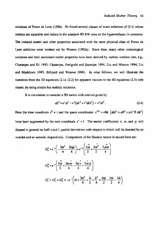
Induced Matter Theory 45
solutions of Ponce de Leon (1988). He found several classes of exact solutions of (2.1) whose
metrics are separable and reduce to the standard 4D RW ones on the hypersurfaces I = constants.
The induced matter and other properties associated with the most physical class of Ponce de
Lcon solutions were worked out by Wesson (1992a). Since then, many other cosmological
solutions and their associated matter properties have been derived by various workers (see, e.g.,
Chatterjee and Sil 1993; Chatterjee, Panigrahi and Banerjee 1994; Liu and Wesson 1994; Liu
and Mashhoon 1995; Billyard and Wesson 1996). In what follows, we will illustrate the
transition from the 5D equations (2.1), (2.2) for apparent vacuum to the 4D equations (2.3) with
matter, by using simple but realistic solutions.
It is convenient to consider a 5D metric with interval given by
dSz =evdt2 -e"(dr2 + r 2 d n 2 ) - e'dl' . (2.4)
Here the time coordinate xo = t and the space coordinates x"' = re$ (dn' = doz +sin2 0 d$')
have been augmented by the new coordinate x4 = I . The metric coefficients v , w , and p will
depend in general on both t and I , partial derivatives with respect to which will be denoted by an
overdot and an asterisk, respectively. Components of the Einstein tensor in mixed form are:
' 1 (z' 4 ' 4 4 G , - e 0 - -" 3w 3 h w 3hv 3wjl
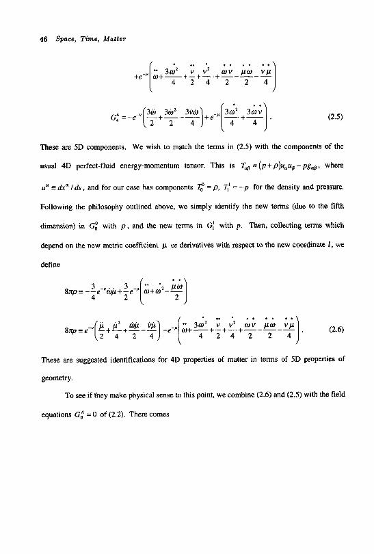
46 Space, Time, Matter
(2.5)
These are 5D components. We wish to match the terms in (2.5) with the components of the
usual 4D perfect-fluid energy-momentum tensor. This is T, = (pi p)uaue - p g d , where
ua e dr" I d s , and for our case has components = p, T,' = - p for the density and pressure.
Following the philosophy outlined above, we simply identify the new terms (due to the fifth
dimension) in G; with p , and the new terms in G: with p. Then, collecting terms which
depend on the new metric coefficient g or derivatives with respect to the new coordinate I , we
define
/ r \
These are suggested identifications for 4D properties of matter in terms of 5D properties of
geometry.
To see if they make physical sense to this point, we combine (2.6) and (2.5) with the field
equations G," = 0 of (2.2). There comes
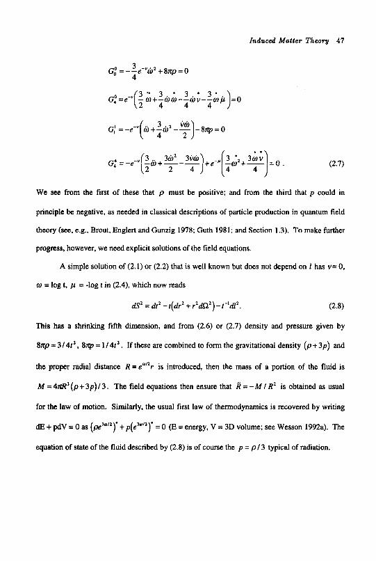
induced Matter Theory 47
3 -
4 G," =--e 'hz+8np=0
(2.7)
We see from the first of these that p must be positive; and from the third that p could in
principle be negative, as needed in classical descriptions of particle production in quantum field
theory (see, e.g., Brout, Englert and Gunzig 1978; Guth 1981; and Section 1.3). To make further
propas, however, we need explicit solutions of the field equations.
A simple solution of (2.1) or (2.2) that is well known but does not depend on I has v= 0,
w = log t, p = -log t in (2.4), which now reads
dSz = dt2 - t(drz + rZdQ2) - t-'dlz. (2.8)
This has a shrinking fifth dimension, and from (2.6) or (2.7) density and pressure given by
81cp=3/4tZ, 8 p = 1/4rZ. If these are combined to form the gravitational density (p+3p) and
the proper radial distance R = e"'r is introduced, then the mass of a portion of the fluid is
M = 4nR3 (p + 3p) I 3 . The field equations then ensure that R = -M / RZ is obtained as usual
for the law of motion. Similarly, the usual first law of thermodynamics is recovered by writing
dE + pdV = 0 as ( j ~ ~ ~ " ) . t p(e'"")' = 0 (E = energy, V = 3D volume; see Wesson 1992a). The
equation of state of the fluid described by (2.8) is of course the p = p/ 3 typical of radiation.
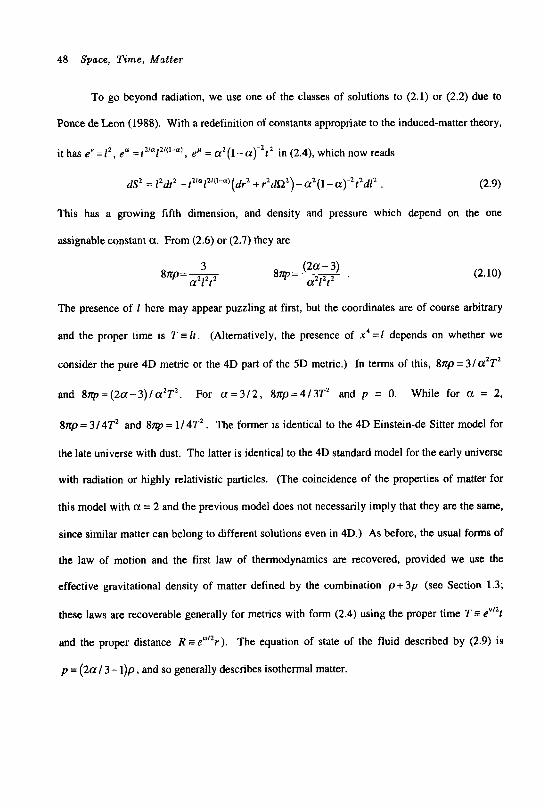
48 Space, Time, Matter
To go beyond radiation, we use one of the classes of solutions to (2.1) or (2.2) due to
Ponce de Leon (1988). With a redefinition of constants appropriate to the induced-matter theory,
it has e" = I z , ew =r2'ulZ'( '-a), e" = aZ(l- a)-'? in (2.4), which now reads
dsz = 12dt2 - r1'a[2'('-a)(&-z + r2dQ2) - a2(1 - a)Jr2d12 . (2.9)
This has a growing fifth dimension, and density and pressure which depend on the one
assignable constant a. From (2.6) or (2.7) they are
(2a - 3) 87p= - aZIZtZ ,
(2.10)
The presence of 1 here may appear puzzling at first, but the coordinates are of course arbitrary
and the proper time is T E Zr . (Alternatively, the presence of x4 = I depends on whether we
consider the pure 4D metric or the 4D part of the 5D metric.) In terms of this, 8np= 3/aZT2
and 8np=(2a-3)la2T2. For a = 3 / 2 , 8np=4/3T2 and p = 0. While for a = 2,
8 ~ p = 3/4T2 and 8p = 1/4TZ. The former is identical to the 4D Einstein-de Sitter model for
the late universe with dust. The latter is identical to the 4D standard model for the early universe
with radiation or highly relativistic particles. (The coincidence of the properties of matter for
this model with a = 2 and the previous model does not necessarily imply that they are the same,
since similar matter can belong to different solutions even in 4D.) As before, the usual forms of
the law of motion and the first law of thermodynamics are recovered, provided we use the
effective gravitational density of matter defined by the combination p + 3 p (see Section 1.3;
these laws are recoverable generally for metrics with form (2.4) using the proper time T = e"'*r
and the proper distance R=e'""r). The equation of state of the fluid described by (2.9) is
p = (2a / 3- 1)p , and so generally describes isothermal matter.
Induced Matter Theory 49
Other properties of (2.9) were studied by Wesson (1992a, 1994). including the sizes of
horizons and the nature of the extra coordinate 1 . We defer further discussion of this model,
because here we are mainly dealing with theoretical aspects of induced-matter theory. However,
we note two things. First, the solutions (2.8) and (2.9) describe in general photons with zero rest
mass and particles with finite rest mass, respectively; and the fact that the former does not
depend on 1 whereas the latter does, gives us a first inkling that 1 is related to mass (see later).
Second, the solution (2.9) gives an excellent description of matter in the late and early universe
from the big-bang perspective of physics in 4D; but it has a somewhat amazing property from the
perspective of geometry in 5D. Thus consider a coordinate transformation from f, r, 1 to T, R, L
specified by
(2.11)
Then (as may be verified by computer) the Ponce de Leon metric (2.9) in standard form becomes
dSz =dTZ-(dR2+R2dS1Z)-dL.z . (2.12)
This means that our universe can either be viewed as a 4D spacetime curved by matter or as a 5D
flat space that is empty.
2.4 The Soliton Case
There is a class of exact solutions of (2.1) which has been rediscovered several times
during the history of Kaluza-Klein theory. The metric is static, spherically-symmetric in
ordinary (3D) space, and independent of the fifth coordinate. (There are many of these solutions
50 Space, Tame, Matter
rather than one because Birkhoff's theorem does not apply in its conventional form in 5D.) The
solutions have been interpreted as describing magnetic monopoles (Sorkin 1983), massive
objects of which some called solitons have no gravitational effect (Gross and Perry 1983). and
black holes (Davidson and Owen 1985). The first usage is questionable, because the 4D
Schwarzschild solution is a special member of the class and gravitational in nature, and magnetic
monopoles are in any case conspicuous by their absence in the real world. The last usage is
misleading, because all but the Schwarzschild-like member of the class lack event horizons of
the conventional sort. The middle usage can be extended, since in the induced-matter picture we
will see that these solutions represent stable, extended objects (Wesson 1992b). Thus even
though the word is over-worked in physics, we regard these 5D 1-body solutions as representing
objects called solitons.
A particularly simple member of the soliton class was rediscovered by Chatterjee (1990).
It is instructive to start with this, because it has been analyzed in standard or Schwarzschild-like
coordinates (as opposed to the isotropic coordinates used below). Thus the 5D metric has an
interval given by
2A ] ' d12 . (2.13)
Here the constant A would normally be identified in gravitational applications via the r + - limit as f i= M., the mass of an object like a star at the centre of ordinary space. However, as
mentioned above, it cannot be assumed that (2.13) is a black hole. Indeed, the first metric
coefficient in (2.13) goes to zero only for r tending to zero. In other words, the event horizon in
the coordinates of (2.13) shrinks to a point at the centre of ordinary space. (This is not altered by
a Killing-vector prescription for horizons and different sets of coordinates: see Wesson and
' -JZ+J;i .
Induced Matter Theory 51
Ponce de Leon 1984.) To see what (2.13) actually represents, let us use the induced-matter
approach. It is helpful to consider a metric we will come back to later, namely
dS2 = e'dt' -eadr2 - R2dQZ -e"d12. (2.14)
This includes (2.13) if we assume that the metric coefficients v , A , R, p depend only on the
radius and not on the time or extra coordinate. Then following the same procedure as in the
preceding section, we obtain the components of the induced 4D energy-momentum tensor :
(2.15)
Here a prime denotes the partial derivative with respect to the radius. Other components are
zero, and of course I;" = r,' because of spherical symmetry. The components (2.15) which
define the properties of matter depend on derivatives of p , that is upon the geometry of the fifth
dimension. However, matter and geometry are unified via the field equations C," = 0 of (2.2),
and we can use these to rewrite (2.15) in a more algebraically convenient form:
8 f 1 ° - - - e - 1 1 -+--- 2R" R'* R'A') 0 - R 2 ( R R2 R
8H,' = - - e 1 - A (x+T) Rt2 R'v' R2
Substituting into these equations for the Chattejee solution (2.13) gives
52 Space, Time, Matter
(2.17)
These components obey the equation of state
q + I ; ’ + q z + + ’ = o , (2.18)
which is radiation-like. The matter described by (2.17) has a gravitational mass that can be
evaluated using the standard 4D expression
M , ( r ) s J(C - q’ - T,’ - q 3 ) 6 d V 3 , (2.19)
where &( is the determinant of the 4-metric and dV, is a 3D volume element. Using (2.14) and
(2.16) this gives
1 2R’v’ 1 v,A, e(“-1)12 7 M,(r) = !. ( vn + - v” + - - - 2 2 R 2 ) R d r (2.20)
This is most conveniently evaluated in the coordinates of the Chatterjee solution in the form
(2.13). Thus putting R + rand integrating gives
1 2 ( v - I ) /Z , M , ( r ) = - r e V , 2
(2.21)
which with the coefficients of (2.13) is
(2.22)
We see that M,(-) = a, agreeing with the usual metric-based definition of the mass as noted
above. However, we also see that M , (0) = 0, meaning that the gravitational mass goes to zero
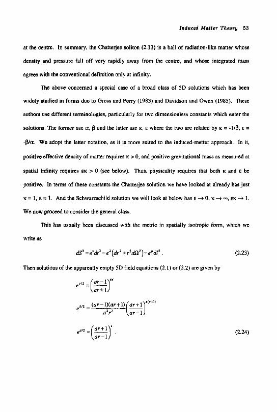
Induced Matter Theory 53
at the centre. In summary, the Chatterjee soliton (2.13) is a ball of radiation-like matter whose
density and pressure fall off very rapidly away from the centre, and whose integrated mass
agrees with the conventionai definition only at infinity.
The above concerned a special case of a broad class of 5D solutions which has been
widely studied in forms due to Gross and Perry (1983) and Davidson and Owen (1985). These
authors use different terminologies, particularly for two dimensionless constants which enter the
solutions. The former use a, Z, and the latter use K, E where the two are related by K = -Up, E =
$/a We adopt the latter notation, as it is more suited to the induced-matter approach. In it,
positive effective density of matter requires K > 0, and positive gravitational mass as measured at
spatial infinity requires EK > 0 (see below). Thus, physicality requires that both K and & be
positive. In terms of these constants the Chatterjee solution we have looked at already has just
K = 1, E = 1. And the Schwanschild solution we will look at below has E + 0, K + -, EK + 1.
We now proceed to consider the general class.
This has usually been discussed with the metric in spatially isotropic form, which we
write as
dS2=e'dt2-eA(dr2+r2dS12)-e'd12 . (2.23)
Then solutions of the apparently empty 5D field equations (2. I ) or (2.2) are given by
(2.24)
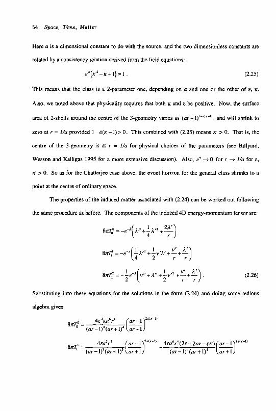
54 Space, Time, Matter
Here a is a dimensional constant to do with the source, and the two dimensionless constants are
related by a consistency relation derived from the field equations:
E ~ ( K ~ - K + I ) = ~ . (2.25)
This means that the class is a 2-parameter one, depending on a and one or the other of E, K.
Also, we noted above that physicality requires that both K and E be positive. Now, the surface
area of 2-shells around the centre of the 3-geometry varies as (ar - l)’-e(K-’), and will shrink to
zero at r = I/a provided 1 - E ( K - 1) > 0. This combined with (2.25) means K 2 0. That is, the
centre of the 3-geometry is at r = l/a for physical choices of the parameters (see Billyard,
Wesson and Kalligas 1995 for a more extensive discussion). Also, e“ + 0 for r + I/a for E ,
K > 0. So as for the Chatterjee case above, the event horizon for the general class shrinks to a
point at the centre of ordinary space.
The properties of the induced matter associated with (2.24) can be worked out following
the same procedure as before. The components of the induced 4D energy-momentum tensor are:
(2.26)
Substituting into these equations for the solutions in the form (2.24) and doing some tedious
algebra gives
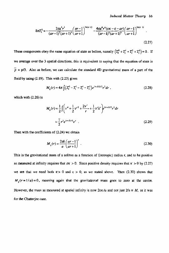
Induced Matter Theory 55
These components obey the same equation of state as before, namely (To + 1;' + qz + q3) = 0. If
we average over the 3 spatial directions, this is equivalent to saying that the equation of state is
p = p/3. Also as before, we can calculate the standard 4D gravitational mass of a part of the
fluid by using (2.19). This with (2.23) gives
-
~ , ( r ) = 4xj(q0 -I;' -I;' - ~ , ~ ) e ' ~ + ~ " ' / ~ r ~ d r , (2.28)
which with (2.26) is
Then with the coefficients of (2.24) we obtain
(2.29)
(2.30)
This is the gravitational mass of a soliton as a function of (isotropic) radius r, and to be positive
as measured at infinity requires that EK > 0. Since positive density requires that K > 0 by (2.27)
we see that we need both K > 0 and E > 0, as we stated above. Then (2.30) shows that
M , ( r = l /a) =0, meaning again that the gravitational mass goes to zero at the centre.
However, the mass as measured at spatial infinity is now 2EKh and not just 2/a I M. as it was
for the Chatterjee case.
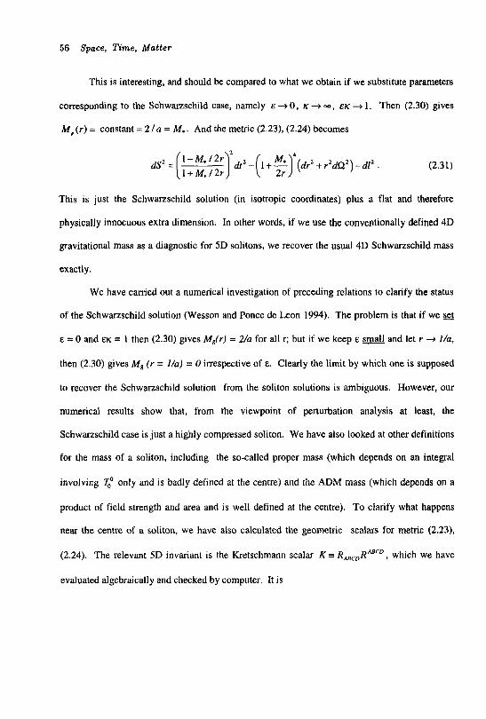
56 Space, T i m e , Matter
This is interesting, and should be compared to what we obtain if we substitute parameters
corresponding to the Schwarzschild case, namely E -+ 0. K -+ -, EK -+ 1 . Then (2.30) gives
M8(r) = constant = 2/u = M.. And the metric (2.23), (2.24) becomes
(2.31)
This is just the Schwarzschild solution (in isotropic coordinates) plus a flat and therefore
physically innocuous extra dimension. In other words, if we use the conventionally defined 4D
gravitational mass as a diagnostic for 5D solitons, we recover the usual 4D Schwarzschild mass
exactly.
We have carried out a numerical investigation of preceding relations to clarify the status
of the Schwarzschild solution (Wesson and Ponce de Leon 1994). The problem is that if we
E = 0 and EK = I then (2.30) gives M,(r) = 2/a for all r; but if we keep E and let r -+ I/u,
then (2.30) gives M, (r = I/u) = 0 irrespective of E. Clearly the limit by which one is supposed
to recover the Schwanschild solution from the soliton solutions is ambiguous. However, our
numerical results show that, from the viewpoint of perturbation analysis at least, the
Schwarzschild case is just a highly compressed soliton. We have also looked at other definitions
for the mass of a soliton, including the so-called proper mass (which depends on an integral
involving only and is badly defined at the centre) and the ADM mass (which depends on a
product of field strength and area and is well defined at the centre). To clarify what happens
near the centre of a soliton, we have also calculated the geometric scalars for metric (2.23),
(2.24). The relevant 5D invariant is the Kretschmann scalar K 5 R,,,RAaCD, which we have
evaluated algebraically and checked by computer. It is
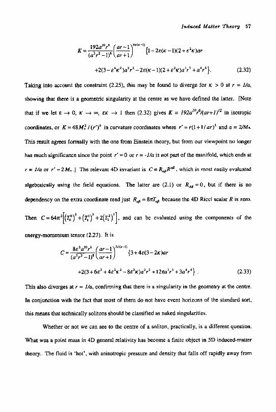
Induced Matter Theory 57
+2(3- &'K2)aZr2 - 2&(K - 1)(2+ EZK)a3r' + a 4 r 4 } . (2.32)
Taking into account the constraint (2.25), this may be found to diverge for K > 0 at r = Z/a,
showing that there is a geometric singularity at the centre as we have defined the latter. [Note
that if we let E + 0, K + m, EK + 1 then (2.32) gives K = Z92a'or6/(ar+~)'2 in isotropic
coordinates, or K = 48M: / (r ' )6 in curvature coordinates where r' = r ( l+ l /ar) ' and a = 2/M*.
This result a g m s formally with the one from Einstein theory, but from our viewpoint no longer
has much significance since the point r' = 0 or r = -Z/a is not part of the manifold, which ends at
r = I/a or r' = 2M. .] The relevant 4D invariant is C E R, R"@ , which is most easily evaluated
algebraically using the field equations. The latter are (2.1) or RAB = 0 , but if there is no
dependency on the extra coordinate read just R, = S m b , because the 4D Ricci scalar R is zero.
Then C = 64n2[(qo)' +(1;')2 +2(q2)2 ] , and can be evaluated using the components of the
energy-momentum tensor (2.27). It is
+ 2 ( 3 + 6 ~ ~ +4&'KZ -8&'K)aZrZ +l2Ea'r' +3a4r4} . (2.33)
This also diverges at r = I/a, confirming that there is a singularity in the geometry at the centre.
In conjunction with the fact that most of them do not have event horizons of the standard sort,
this means that technically solitons should be classified as naked singularities.
Whether or not we can see to the centre of a soliton, practically, is a different question.
What was a point mass in 4D general relativity has become a finite object in 5D induced-matter
theory. The fluid is 'hot', with anisotropic pressure and density that falls off rapidly away from
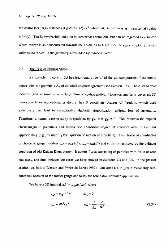
58 Space, Tame, Matter
the centre (for large distances it goes as M.2 / r4 where M. is the mass as measured at spatial
infinity). The Schwarzschild solution is somewhat anomalous, but can be regarded as a soliton
where matter is so concentrated towards the centre as to leave most of space empty. In short,
solitons are ‘holes’ in the geometry surrounded by induced matter.
2.5 The Case of Neutral Matter
Kaluza-Klein theory in 5D has traditionally identified the ha components of the metric
tensor with the potentials A, of classical electromagnetism (see Section 1.5). These set to zero
therefore give in some sense a description of neutral matter. However, any fully covariant 5D
theory, such as induced-matter theory, has 5 coordinate degrees of freedom, which used
judiciously can lead to considerable algebraic simplification without loss of generality.
Therefore, a natural case to study is specified by g4a = 0, 944 f 0. This removes the explicit
electromagnetic potentials and leaves one coordinate degree of freedom over to be used
appropriately (e.g., to simplify the equation of motion of a particle). This choice of coordinates
or choice of gauge involves gap = gap (x*), &24 = &24(xA) and so is not restricted by the cylinder
condition of old Kaluza-Klein theory. It admits fluids consisting of particles with finite or zero
rest mass, and thus includes the cases we have studied in Sections 2.3 and 2.4. In the present
section, we follow Wesson and Ponce de Leon (1992). Our aims are to give a reasonably self-
contained account of the matter gauge and to lay the foundation for later applications.
We have a 5D interval dSz = gA,drAdrB where
g@ = g,fxA) g4, = 0
(2.34)
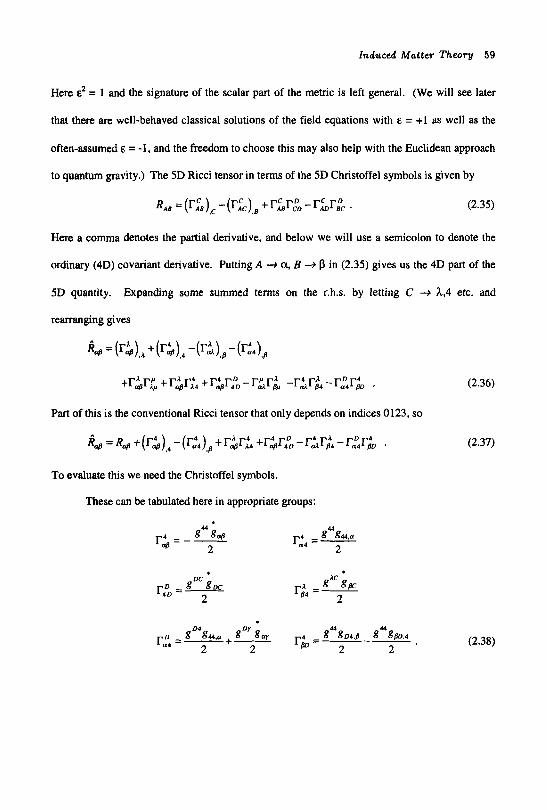
Induced Matter Theory 59
Here E* = 1 and the signature of the scalar part of the metric is left general. (We will see later
that there are well-behaved classical solutions of the field equations with E = +1 as well as the
often-assumed E = -1, and the freedom to choose this may also help with the Euclidean approach
to quantum gravity.) The 5D Ricci tensor in terms of the 5D Christoffel symbols is given by
R.4B -(r,k),B + r ~ B r ~ D - r ~ D r ~ C ' (2.35)
Here a comma denotes the partial derivative, and below we will use a semicolon to denote the
ordinary (4D) covariant derivative. Putting A + a, E + in (2.35) gives us the 4D part of the
5D quantity. Expanding some summed terms on the r.h.s. by letting C + h,4 etc. and
rearranging gives
i d = (G),, +RJ4 -(rA),@ -(r:4),$
+r$r& + r$r;4 + r$-fD - r$rh -rAri4 - r:4r& . (2.36)
Part of this is the conventional Ricci tensor that only depends on indices 0123, so
id = R~ + ( r$),4 - ( r:4),, + r$r;, +r$rpD - r;ri4 - r;riD . (2.37)
To evaluate this we need the Christoffel symbols.
These can be tabulated here in appropriate groups:
44 g g44.a r:4 = -
2
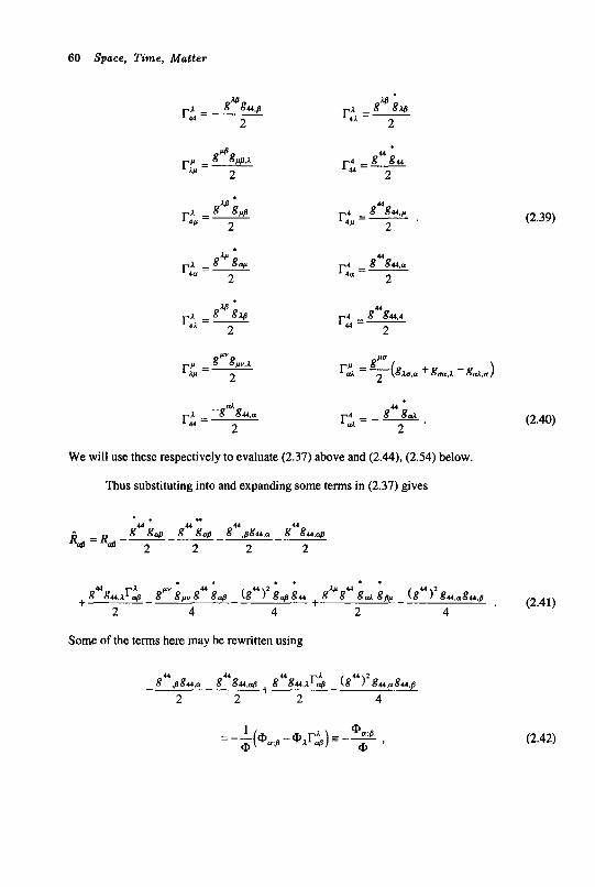
60 Space, Time, Matter
(2.39)
(2.40)
We will use these respectively to evaluate (2.37) above and (2.44), (2.54) below.
Thus substituting into and expanding some terms in (2.37) gives
Some of the terms here may be rewritten using
(2.42)
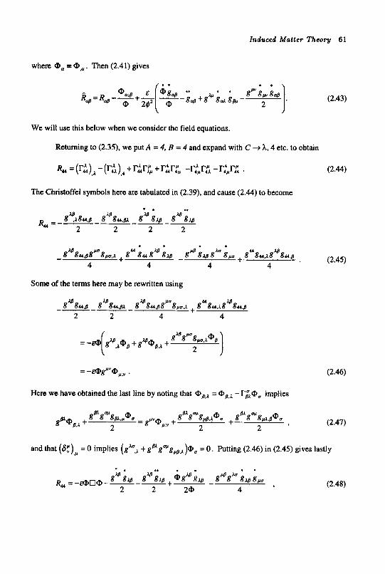
Induced Matter Theory 61
We will use this below when we consider the field equations.
Returning to (2.35), we put A = 4, B = 4 and expand with C + h, 4 etc. to obtain
R, = (r:),, - (r;,),, + r:r& + r:r& -r;,r:, - r&r& . (2.44)
The Christoffel symbols here are tabulated in (2.39), and cause (2.44) to become
L L L
Some of the terns here may be rewritten using
“ I
= -ag’”#,;” . (2.46)
Hex we have obtained the last line by noting that = O,, - r i O 0 implies
and that (6;) = 0 implies (gasqa + gPgqg,,,)@., = 0 . Putting (2.46) in (2.45) gives lastly 1,
(2.48)
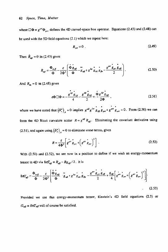
62 Space, Time, Matter
where El@ 3 g""@,;, defines the 4D curved-space box operator. Equations (2.43) and (2.48) can
be used with the 5D field equations (2.1) which we repeat here:
R,, = 0 . (2.49)
Then R, = 0 in (2.43) gives
And R4 = 0 in (2.48) gives
(2.50)
(2.51)
1 . * . where we have noted that (St),, = 0 implies g'gAu gv g,, t gPu gPu = 0 . From (2.50) we can
form the 4D Ricci curvature scalar R = g@ R,. Eliminating the covariant derivative using
(2.51), and again using (S:),4 = 0 to eliminate some terms, gives
R = ~ [ g ; ' ~ , , + ( g " v ~ p y ) l ] 4@ . (2.52)
With (2.50) and (2.52), we are now in a position to define if we wish an energy-momentum
tensor in 4D via 8nT, I R, - Rg+ I2. It is
. (2.53)
Provided we use this energy-momentum tensor, Einstein's 4D field equations (2.3) or
Gab = 8 f l 4 will of course be satisfied.
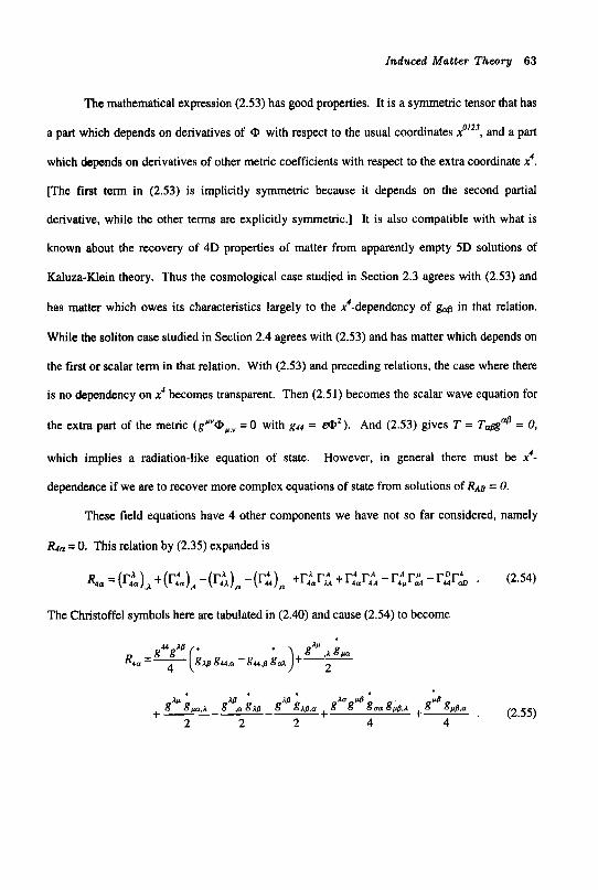
Induced Matter Theory 63
The mathematical expression (2.53) has good properties. It is a symmetric tensor that has
a part which depends on derivatives of CJ with respect to the usual coordinates xoiZ3, and a part
which depends on derivatives of other metric coefficients with respect to the extra coordinate 2.
[The first term in (2.53) is implicitly symmetric because it depends on the second partial
derivative, while the other terms are explicitly symmetric.] It is also compatible with what is
known about the recovery of 4D properties of matter from apparently empty 5D solutions of
Kaluza-Klein theory. Thus the cosmological case studied in Section 2.3 agrees with (2.53) and
has matter which owes its characteristics largely to the x4-dependency of gM in that relation.
While the soliton case studied in Section 2.4 agrees with (2.53) and has matter which depends on
the first or scalar term in that relation. With (2.53) and preceding relations, the case where there
is no dependency on x4 becomes transparent. Then (2.51) becomes the scalar wave equation for
the extra part of the metric (gv'CJp,y = 0 with g44 = &*). And (2.53) gives T = = 0,
which implies a radiation-like equation of state. However, in general there must be x4-
dependence if we are to recover more complex equations of state from solutions of RAB = 0.
These field equations have 4 other components we have not so far considered, namely
Rda = 0. This relation by (2.35) expanded is
The Christoffel symbols here are tabulated in (2.40) and cause (2.54) to become
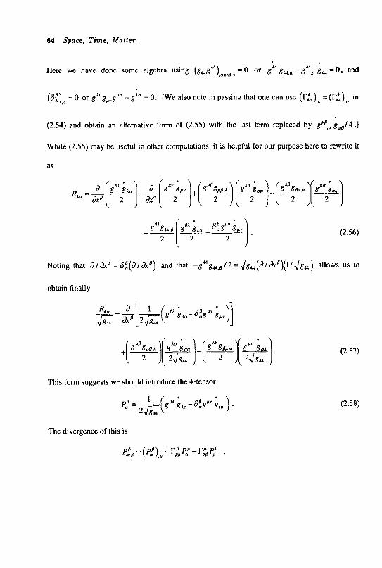
64 Space, Time, Matter
44 44 Here we have done some algebra using (g,g44),umd4 = 0 or g - g ,a g, = 0 , and
(6f),4 = 0 or gA”gpvgp“ +gA“ = 0 . [We also note in passing that one can use (r:a),r = (r:) .a in
(2.54) and obtain an alternative form of (2.55) with the last term replaced by g”p,a g,/4 .]
While (2.55) may be useful in other computations, it is helpful for our purpose here to rewrite it
as
This form suggests we should introduce the 4-tensor
(2.57)
(2.58)
The divergence of this is
P;, =(~:),~+r,p:-rp; ,
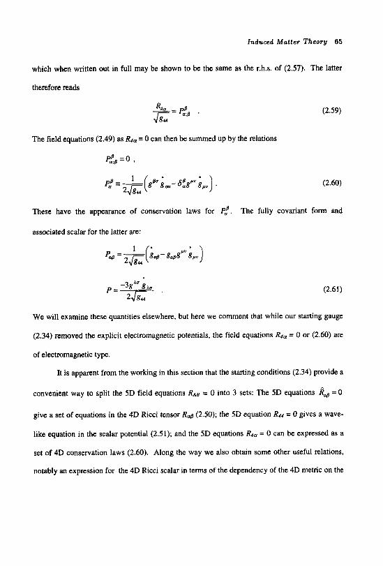
Induced Matter Theory 65
which when written out in full may be shown to be the same as the r.h.s. of (2.57). The latter
therefore reads
The field equations (2.49) as R4= = 0 can then be summed up by the relations
p:,=o 1
(2.59)
(2.60)
These have the appearance of conservation laws for P!. The fully covariant form and
associated scalar for the latter are:
(2.61)
We will examine these quantities elsewhere, but here we comment that while our starting gauge
(2.34) removed the explicit electromagnetic potentials, the field equations Rda = 0 or (2.60) are
of electromagnetic type.
It is apparent from the working in this section that the starting conditions (2.34) provide a
convenient way to split the 5D field equations RAB = 0 into 3 sets: The 5D equations &, = 0
give a set of equations in the 4D Ricci tensor RM (2.50); the 5D equation R44 = 0 gives a wave-
like equation in the scalar potential (2.51); and the 5D equations R4a = 0 can be expressed as a
set of 4D conservation laws (2.60). Along the way we also obtain some other useful relations,
notably an expression for the 4D Ricci scalar in terms of the dependency of the 4D metric on the
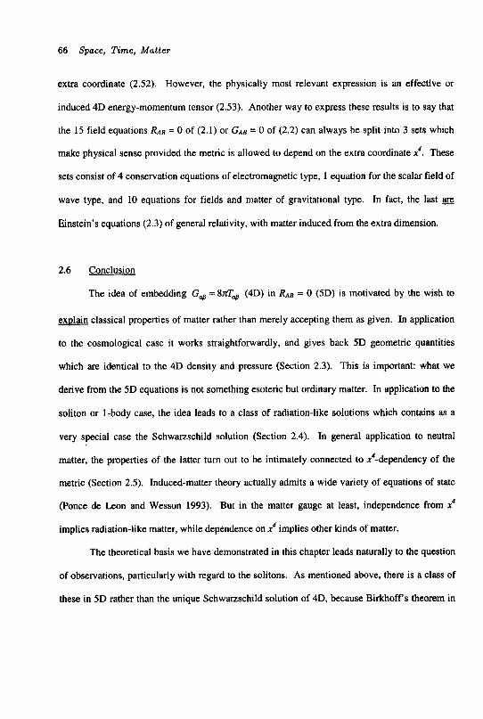
66 Space, Time, M a t t e r
extra coordinate (2.52). However, the physically most relevant expression is an effective or
induced 4D energy-momentum tensor (2.53). Another way to express these results is to say that
the 15 field equations RAE = 0 of (2.1) or GAB = 0 of (2.2) can always be split into 3 sets which
make physical sense provided the metric is allowed to depend on the extra coordinate x4. These
sets consist of 4 conservation equations of electromagnetic type, 1 equation for the scalar field of
wave type, and 10 equations for fields and matter of gravitational type. In fact, the last are
Einstein's equations (2.3) of general relativity, with matter induced from the extra dimension.
2.6 Conclusion
The idea of embedding G , = 8mb, (4D) in RAE = 0 (5D) is motivated by the wish to
exDlain classical properties of matter rather than merely accepting them as given. In application
to the cosmological case it works straightforwardly, and gives back 5D geometric quantities
which are identical to the 4D density and pressure (Section 2.3). This is important: what we
derive from the 5D equations is not something esoteric but ordinary matter. In application to the
soliton or 1-body case, the idea leads to a class of radiation-like solutions which contains as a
very special case the Schwarzschild solution (Section 2.4). In general application to neutral
matter, the properties of the latter turn out to be intimately connected to x4-dependency of the
metric (Section 2.5). Induced-matter theory actually admits a wide variety of equations of state
(Ponce de Leon and Wesson 1993). But in the matter gauge at least, independence from x4
implies radiation-like matter, while dependence on x4 implies other kinds of matter.
The theoretical basis we have demonstrated in this chapter leads naturally to the question
of observations, particularly with regard to the solitons. As mentioned above, there is a class of
these in 5D rather than the unique Schwarzschild solution of 4D, because Birkhoff's theorem in
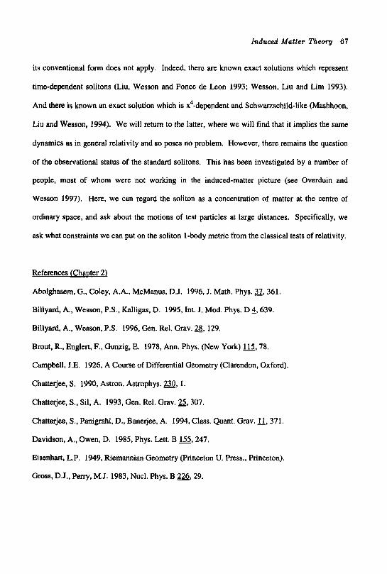
Induced Matter Theory 67
its conventional form does not apply. Indeed, there are known exact solutions which represent
time-&pendent solitons (Liu, Wesson and Ponce de Leon 1993; Wesson, Liu and Lim 1993).
And there is known an exact solution which is x4-dependent and Schwarzschild-like (Mashhoon,
Liu and Wesson, 1994). We will return to the latter, where we will find that it implies the same
dynamics as in general relativity and so poses no problem. However, there remains the question
of the observational status of the standard solitons. This has been investigated by a number of
people, most of whom were not working in the induced-matter picture (see Overduin and
Wesson 1997). Here, we can regard the soliton as a concentration of matter at the centre of
ordinary space, and ask about the motions of test particles at large distances. Specifically, we
ask what constraints we can put on the soliton 1-body metric from the classical tests of relativity.
References (Chauter 2)
Abolghasem, G., Coley, A.A., McManus, D.J. 1996, J. Math. Phys. 22,361.
Billyard, A., Wesson, P.S., Kalligas, D. 1995, Int. I. Mod. Phys. D 4,639.
Billyard, A., Wesson, P.S. 1996, Gen. Rel. Grav. 28, 129.
Brout, R., Englert, F., Gunzig, E. 1978, Ann. Phys. (New York) m,78.
Campbell, J.E. 1926, A Course of Differential Geometry (Clarendon, Oxford).
Chattejee, S. 1990, Astron. Astrophys. 230, 1.
Chattejec, S., Sil, A. 1993, Gen. Rel. Grav. 2,307.
Chattejee, S., Panigrahi, D., Banerjee, A. 1994, Class. Quant. Grav. 1.371.
Davidson, A., Owen, D. 1985, Phys. Lett. B 155,247.
Eisenhart, L.P. 1949, Riemannian Geometry (Princeton U. Press., Princeton).
Gross, D.J., Perry, M.J. 1983, Nucl. Phys. B 226, 29.
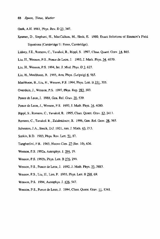
68 Space, Time, Matter
Guth, A.H. 1981, Phys. Rev. D 2 , 3 4 7 .
Kramer, D., Stephani, H., MacCallum, M., Herlt, E. 1980, Exact Solutions of Einstein’s Field
Equations (Cambridge U. Press, Cambridge).
Lidsey, J.E., Romero, C., Tavakol, R., Rippl, S. 1997, Class. Quant. Grav. 14,865.
Liu, H., Wesson, P.S., Ponce de Leon, J. 1993, J. Math. Phys. 34,4070.
Liu, H., Wesson, P.S. 1994, Int. J. Mod. Phys. D 3,627.
Liu, H., Mashhoon, B. 1995, Ann. Phys. (Leipzig) 4,565.
Mashhoon, B., Liu, H., Wesson, P.S. 1994, Phys. Lett. B 331, 305.
Overduin, J., Wesson, P.S. 1997, Phys. Rep. 283,303.
Ponce de Leon, J. 1988, Gen. Rel. Grav. 20,539.
Ponce de Leon, J., Wesson, P.S. 1993, J. Math. Phys. 3 ,4080.
Rippl, S . , Romero, C., Tavakol, R. 1995, Class. Quant. Grav. l2,2411.
Romero, C., Tavakol. R., Zalaletdinov, R. 1996, Gen. Rel. Grav. 3, 365.
Schouten, J.A., Struik, D.J. 1921, Am. J. Math. 43, 213.
Sorkin, R.D. 1983, Phys. Rev. Lett. 5l,87.
Tangherlini, F.R. 1963, Nuovo Cim. 21 (Ser. lo), 636.
Wesson, P.S. 1992a, Astrophys. J. 394, 19.
Wesson, P.S. 1992b, Phys. Lett. B 276,299.
Wesson, P.S., Ponce de Leon, J. 1992, J. Math. Phys. 33,3883.
Wesson, P.S., Liu, H., Lim, P. 1993, Phys. Lett. B =,69.
Wesson, P.S. 1994, Astrophys. J. 436,547.
Wesson, P.S., Ponce de Leon, J. 1994, Class. Quant. Grav. ll, 1341.
3. THE CLASSICAL AND OTHER TESTS IN 5D
“You need to be constrained” (Clifford Will, St. Louis, 1992)
3.1 Introduction
Irrespective of which interpretation one makes of 5D general relativity, the observational
status of the soliton or I-body solutions is central. The classical tests of relativity involve the 4D
Schwarzschild solution applied to the solar system. These include the perihelion advance of
Mercury, the gravitational redshift effect, and the deflection of light by the Sun. To these were
added the time-delay (or radar-ranging) test for electromagnetic radiation passing near the Sun,
and more recently the change due to gravitational radiation of the orbital dynamics of the binary
pulsar system. Einstein’s 4D theory agrees with data on these things, in some cases to an
accuracy of order 0.1% (AdIer, Bazin and Schiffer 1975; Will 1992). Kaluza-Klein 5D theory
can obviously be constrained by these data. However, it also leads to new tests involving the
geodetic precession of a gyroscope. and possible departures from the equivalence principle, both
of which can be tested by spacecraft experiments.
In this chapter, we treat the 5D dynamics of the class of soliton solutions examined in the
preceding chapter. We proceed by first putting the 5D metric into a form that resembles the 4D
one. Then because it is the physically most interesting case, we look at the orbits of photons.
After, we treat the orbits of massive particles and the perihelion advance problem, followed by
the gravitational redshift effect. There follow two sections that deal, respectively, with the
precession of a spinning object in 4D and 5D, and the status of the 4D equivalence principle
versus 5D geodesic motion.
3.2 The I-Bodv Metric
In 4D, the Schwarzschild solution is given in its usual and (3D) isotropic forms by
69
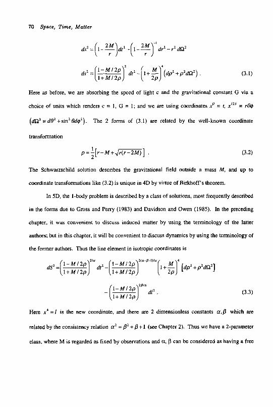
70 Space, Time, Matter
Here as before, we are absorbing the speed of light c and the gravitational constant G via a
choice of units which renders c = 1, G = 1; and we are using coordinates xo = f, xI2 j = t-04
(dQ’ = d o Z +sinZ I%@’). The 2 forms of (3 .1) are related by the well-known coordinate
transformation
p = ’ [ r - M + J - ] 2 . (3.2)
The Schwarzschild solution describes the gravitational field outside a mass M , and up to
coordinate transformations like (3.2) is unique in 4D by virtue of Birkhoff‘s theorem.
In 5D, the 1-body problem is described by a class of solutions, most frequently described
in the forms due to Gross and Perry (1983) and Davidson and Owen (1985). In the preceding
chapter, it was convenient to discuss induced matter by using the terminology of the latter
authors; but in this chapter, it will be convenient to discuss dynamics by using the terminology of
the former authors. Thus the line element in isotropic coordinates is
Here x4 = 1 is the new coordinate, and there are 2 dimensionless constants 01,8 which are
related by the consistency relation a’ = 8’ + p + 1 (see Chapter 2). Thus we have a 2-parameter
class, where M is regarded as fixed by observations and a, p can be considered as having a free
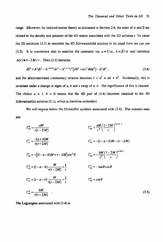
The Classical and Other Tests in 5 0 71
range. (However, for induced-matter theory as discussed in Section 2.4, the sizes of a and fl are
related to the density and pressure of the 4D matter associated with the 5D solution.) To cause
the 5D solutions (3.3) to resemble the 4D Schwarzschild solution in its usual form we can use
(3.2). It is convenient also to redefine the constants via a = l / a , b = f l / a and introduce
A(r) P 1 - 2 M I r . Then (3.3) becomes
(3.4)
and the aforementioned consistency relation becomes 1 = uz + ab + b2. Incidentally, this is
invariant under a change in signs of a, b and a swap of a, b. The significance of this is obscure.
The choice a = 1, b = 0 means that the 4D part of (3.4) becomes identical to the 4D
Schwanschild solution (3.1), which is therefore embedded.
ds2 =A"dt2 -A-(a+b)drZ -Al-n-b r 2 (d#+sin2 & i @ * ) - ~ ~ d P ,
We will require below the Christoffel symbols associated with (3.4). The nonzero ones
are:
aM rp, = r(r - 2 M )
-(a + b)M r;, = r (r - 2M)
r:, = - (1 - a - b)M - ( r - 2M)
M 1 r ( r - 2 M ) r
r: = ( l - u - b ) - +- r;3 = - sin 6 cos 8
r;3 = cot6 M I r ( r - 2 M ) r
r;: = ( ~ - ~ - b ) - +-
bM r ( r - 2 M )
I-;=----.
The Lagrangian associated with (3.4) is
(3.5)
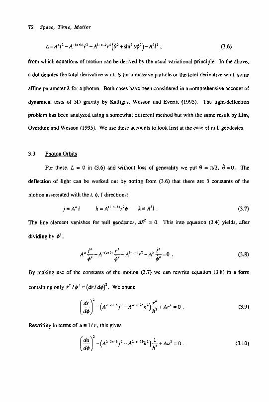
72 Space, Time, Matter
from which equations of motion can be derived by the usual variational principle. In the above,
a dot denotes the total derivative w.r.t. S for a massive particle or the total derivative w.r.t. some
affine parameter h for a photon. Both cases have been considered in a comprehensive account of
dynamica! tests of 5D gravity by Kalligas, Wesson and Everitt (1995). The light-deflection
problem has been analyzed using a somewhat different method but with the same result by Lim,
Overduin and Wesson (1995). We use these accounts to look first at the case of null geodesics.
3.3 Photon Orbits
For these, L = 0 in (3.6) and without loss of generality we put 9 = d 2 , b=O. The
deflection of light can be worked out by noting from (3.6) that there are 3 constants of the
motion associated with the t, 4, 1 directions:
(3.7) j ~ j h ~ A(1-n-b) r 2 4 k s A b i .
The line element vanishes for null geodesics, dS2 = 0. This into equation (3.4) yields, after
dividing by @ ,
By making use of the constants of the motion (3.7) we can rewrite equation (3.8) in a form
containing only i2 / 4' = (dr / de)'. We obtain
Rewriting in terms of u = 1 / r , this gives
(3.9)
(3.10)
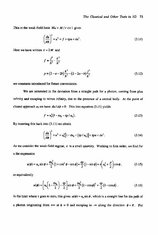
The Classical and Other Testa in 5 0 73
This in the weak-field limit Mu = M / r cc 1 gives
($)’+d = f + 4 , u + a c 3
Here we have written E = 2 M and
.2 2 f =L-k
h’ h2
p (2 -(I - 2 q T k Z - (2 - 2a -b) - j’ h h2
(3.11)
(3.12)
are constants introduced for future convenience.
We are interested in the deviation from a straight path for a photon, coming from plus
infinity and escaping to minus infinity, due to the presence of a central body. At the point of
closest approach uo we have du Id$ = 0 . This into equation (3.11) yields
f = ~ ( l - a c o - c p l u J . (3.13)
By inserting this back into (3.1 1) we obtain
(3.14)
As we consider the weak-field regime, E is a small quantity. Working to first order, we find for
u the expression
4 4, u(4) = uo sin 4 +-(I + cos2 0 -sin 4) +-(I - sin 4) + E 2 2
or equivalently
(3.15)
(3.16)
In the limit where E goes to zero, this gives u($) = uo sin $, which is a straight line for the path of
a photon originating from +oo at $I = 0 and escaping to -m along the direction $ = n. For
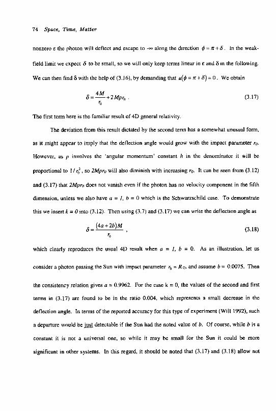
74 Space, Time, Matter
nonzero E the photon will deflect and escape to -- along the direction @ = R + 6 . In the weak-
field limit we expect 6 to be small, so we will only keep terms linear in E and S in the following.
We can then find S with the help of (3.16), by demanding that u(# = + 6) = 0. We obtain
4 M
‘0
6 = -+ 2 Mpr, (3.17)
The first term here is the familiar result of 4D general relativity.
The deviation from this result dictated by the second term has a somewhat unusual form,
as it might appear to imply that the deflection angle would grow with the impact parameter ro.
However, as p involves the ‘angular momentum’ constant h in the denominator it will be
proportional to 1 I r,’ , so 2Mpr0 will also diminish with increasing ro. It can be seen from (3.12)
and (3.17) that 2Mpr0 does not vanish even if the photon has no velocity component in the fifth
dimension, unless we also have a = I, b = 0 which is the Schwarzschild case. To demonstrate
this we insert k = 0 into (3.12). Then using (3.7) and (3.17) we can write the deflection angle as
(3.18) (4a + 2b)M
‘0
6 =
which clearly reproduces the usual 4 D result when a = 1, b = 0. As an illustration, let us
consider a photon passing the Sun with impact parameter ro = R o , and assume b = 0.0075. Then
the consistency relation gives a = 0.9962. For the case k = 0, the values of the second and first
terms in (3.17) are found to be in the ratio 0.004, which represents a small decrease in the
deflection angle. In terms of the reported accuracy for this type of experiment (Will 1992). such
a departure would be j~& detectable if the Sun had the noted value of b. Of course, while b is a
constant it is not a universal one, so while it may be small for the Sun it could be more
significant in other systems. In this regard, it should be noted that (3.17) and (3.18) allow not
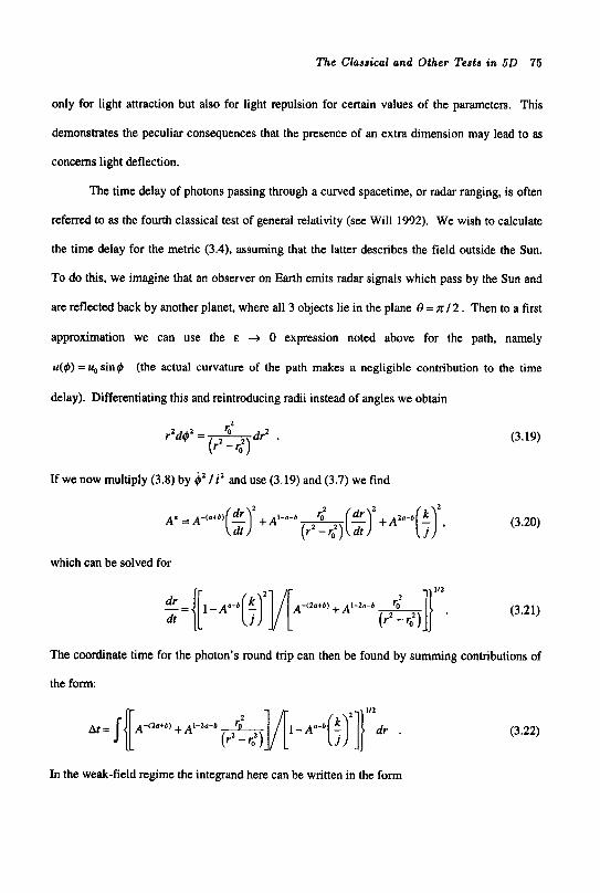
The Classical and Other Tests in 5 0 75
only for light attraction but also for light repulsion for certain values of the parameters. This
demonstrates the peculiar consequences that the presence of an extra dimension may lead to as
concerns light deflection.
The time delay of photons passing through a curved spacetime, or radar ranging, is often
referred to as the fourth classical test of general relativity (see Will 1992). We wish to calculate
the time delay for the metric (3.4). assuming that the latter describes the field outside the Sun.
To do this, we imagine that an observer on Earth emits radar signals which pass by the Sun and
are reflected back by another planet, where all 3 objects lie in the plane 0 = n 1 2 . Then to a first
approximation we can use the E + 0 expression noted above for the path, namely
u ( 0 ) = u, sing (the actual curvature of the path makes a negligible contribution to the time
delay). Differentiating this and reintroducing radii instead of angles we obtain
rz ( 2 - 5 ) r’d9’ = o d r z .
If we now multiply (3.8) by Ii’ and use (3.19) and (3.7) we find
which can be solved for
(3.19)
(3.20)
The coordinate time for the photon’s round trip can then be found by summing contributions of
the form:
(3.22)
In the weak-field regime the integrand here can be written in the form
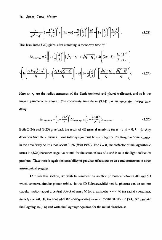
76 Space, Time, Matter
I+(;]
This back into (3.22) gives, after summing, a round trip time of
!$} (3.23)
(3.24)
Here rE, r, are the radius measures of the Earth (emitter) and planet (reflector), and ro is the
impact parameter as above. The coordinate time delay (3.24) has an associated proper time
delay
Both (3.24) and (3.25) give back the result of 4D general relativity for a = 1, b = 0, k = 0. Any
deviation from these values in our solar system must be such that the resulting fractional change
in the time delay be less than about 0.1% (Will 1992). Fork = 0, the prefactor of the logarithmic
terms in (3.24) becomes negative or null for the same values of a and b as in the light-deflection
problem. Thus there is again the possibility of peculiar effects due to an extra dimension in other
astronomical systems.
To finish this section, we wish to comment on another difference between 4D and 5D
which concerns circular photon orbits. In the 4D Schwarzschild metric, photons can be set into
circular motion about a central object of mass M for a particular value of the radial coordinate,
namely r = 3M. To find out what the corresponding value is for the 5D metric (3.4), we can take
the Lagrangian (3.6) and write the Lagrange equation for the radial direction as
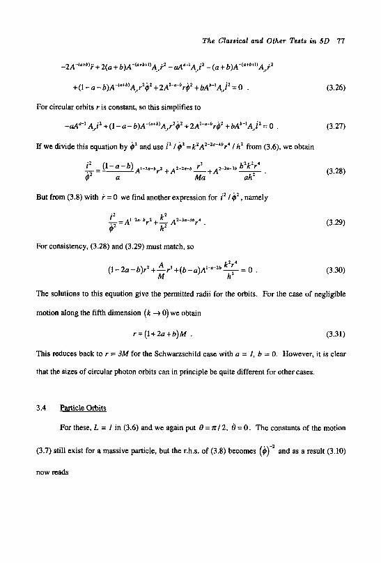
The Classical and Other Tests in 5 0 77
-2A-("+b)f + 2(a + b)A-(aibrl)A.,iZ - &"-lA,,iz - (a .+ b)A-(cltb+l)A,r+Z
+(1 -a - b)A-(ntb)A,,r2$2 +2A'-'-br@ + bAb-'A,,i' = 0 .
For circular orbits r is constant, so this simplifies to
-cut"-' A,,? +(I - a- b)A-(a+b)A,,r2d2 +2A1-"'br$2 + bAb-'A,,12 = 0 .
If we divide this equation by $' and use 1' I 4' = kZA2-Z"~4br' I h' from (3.6), we obtain
But from (3.8) with i = 0 we find another expression for i2 I @ , namely
For consistency, (3.28) and (3.29) must match, so
A kZr4 M h'
(1-2a-b)r2+-r'+(b-a)A'~"-Zb- = 0
(3.26)
(3.27)
(3.28)
(3.29)
(3.30)
The solutions to this equation give the permitted radii for the orbits. For the case of negligible
motion along the fifth dimension (k + 0) we obtain
r=(l+Za+b)M . (3.31)
This reduces back to r = 3M for the Schwarzschild case with a = I , b = 0. However, it is clear
that the sizes of circular photon orbits can in principle be quite different for other cases.
3.4 Particle Orbits
For these, L = J in (3.6) and we again put i3 = n 12, b = 0. The constants of the motion
(3.7) still exist for a massive particle, but the r.h.s. of (3.8) becomes ($)-' and as a result (3.10)
now mads
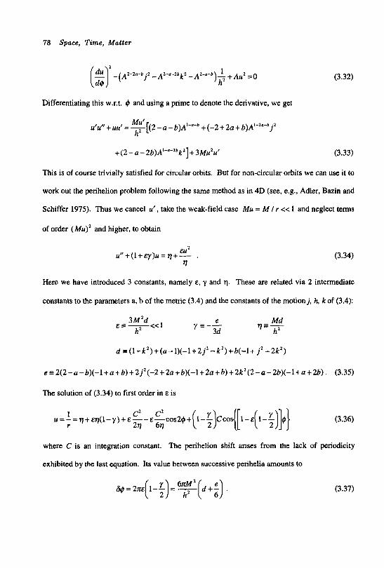
78 Space, Tame, Matter
(3.32)
Differentiating this w.r.t. 4 and using a prime to denote the derivative, we get
Mu' h
u'u" + uu' = ,[(2 - a - b)A'-"-b + (-2 + 2a + b)A1-Z"-bjZ
+(2-a-2b)Al-"~Zbk']+3Mu'u' (3.33)
This is of course trivially satisfied for circular orbits. But for non-circular orbits we can use it to
work out the perihelion problem following the same method as in 4D (see, e.g., Adler, Bazin and
Schiffer 1975). Thus we cancel u' , take the weak-field case Mu = M I r << 1 and neglect terms
of order (Mu)2 and higher, to obtain
(3.34) Elaz
f u " + ( l + & y ) U = q + - .
Here we have introduced 3 constants, namely E, y and q. These are related via 2 intermediate
constants to the parameters a, b of the metric (3.4) and the constants of the motion j, h, k of (3.4):
e Md q'- &E- YE-- 3d hZ 3 M Z d
h'
d E ( 1 + k 2 ) + ( a - 1)(-1+2jz -k ' )+b( - l+ j' - 2 k Z )
e = 2 ( 2 - a - b ) ( - l + a + b ) + 2 j Z ( - 2 + 2 a +b)(- l+Za + b ) + 2 k 2 ( 2 - a -2b ) ( - l+a +B).
The solution of (3.34) to first order in E is
(3.35)
(3.36)
where C is an integration constant. The perihelion shift arises from the lack of periodicity
exhibited by the last equation. Its value between successive perihelia amounts to
(3.37)
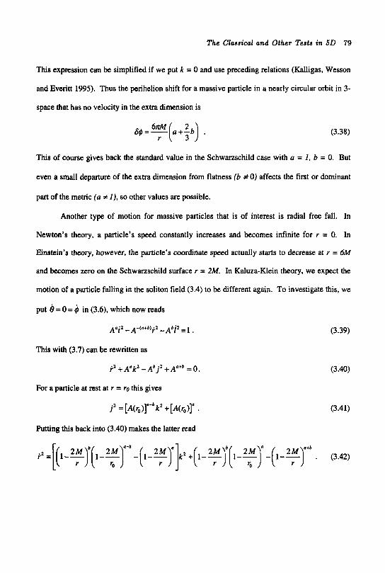
The Classical and Other Tests in 5 0 79
This expression can be simplified if we put k = 0 and use preceding relations (Kalligas, Wesson
and Everitt 1995). Thus the perihelion shift for a massive particle in a nearly circular orbit in 3-
space that has no velocity in the extra dimension is
&==(a+!b) . (3.38)
This of course gives back the standard value in the Schwanschild case with a = I, b = 0. But
even a small departure of the extra dimension from flatness (b # 0) affects the first or dominant
part of the metric (a # I), so other values are possible.
Another type of motion for massive particles that is of interest is radial free fall. In
Newton's theory, a particle's speed constantly increases and becomes infinite for r = 0. In
Einstein's theory, however, the particle's coordinate speed actually starts to decrease at r = 6M
and becomes zero on the Schwanschild surface r = 2M. In Kaluza-Klein theory, we expect the
motion of a particle falling in the soliton field (3.4) to be different again. To investigate this, we
put b = 0 = 4 in (3.6), which now reads
A a i 2 - A-(n+b)fZ - biz = 1 .
This with (3.7) can be rewritten as
Fa +A"k3 - Ab j' =o.
For a particle at rest at r = ro this gives
j' = [ ~ ( r ~ ) ] " - * k ~ +[A(%)]" .
Putting this back into (3.40) makes the latter read
(3.39)
(3.40)
(3.41)

80 Space, Time, Matter
This can be thought of as an energy equation for our problem. Indeed, it is easily seen that in the
limit where n = 1, b = 0, k = 0 it reduces to r2 I2 = M ( 1 I r - 1 I ro) , which is the corresponding
expression for the Schwarzschild case in Einstein's theory and has the same form as the energy
equation in Newton's theory. In Kaluza-Klein theory, the coordinate velocity in the r direction is
dr - dr dS dt ds dt
The second factor here can be written using (3.7) and (3.41) as
- _ "-( dt 1 - - 2 ; y / p J q q
The first factor can be written using (3.42) as
d r l dS = - { [ ( 1 - 2Ml r ) * ( l - 2 M l ray-* - ( 1 - 2M I r)"]k2
The combination means (3.43) becomes
(3.43)
For a particle starting at an infinite radial distance from the central body, this implies
(3.44)
(3.45)
(3.46)
. (3.47)
One feature of this result is that the radial speed of a test particle will depend on its velocity
component along the fifth dimension (through k). In situations where the latter cannot be
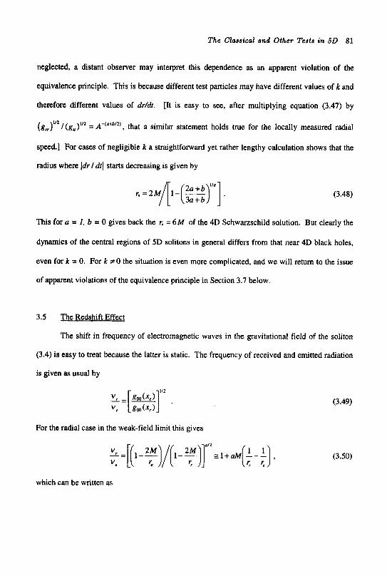
The Classical and Other Tests in 5 0 81
neglected, a distant observer may interpret this dependence as an apparent violation of the
equivalence principle. This is because different test particles may have different values of k and
therefore different values of dr/dr. [It is easy to see, after multiplying equation (3.47) by
(g")'" /(g,,)'" = A-(otb'2), that a similar statement holds true for the locally measured radial
speed.] For cases of negligible k a straightforward yet rather lengthy calculation shows that the
radius where Jdr I drJ starts decreasing is given by
(3.48)
This for a = I, b = 0 gives back the r, = 6M of the 4D Schwarzschild solution. But clearly the
dynamics of the central regions of 5D solitons in general differs from that near 4D black holes,
even for k = 0. For k f 0 the situation is even more complicated, and we will return to the issue
of apparent violations of the equivalence principle in Section 3.7 below.
3.5 The Redshift Effect
The shift in frequency of electromagnetic waves in the gravitational field of the soliton
(3.4) is easy to treat because the latter is static. The frequency of received and emitted radiation
is given as usual by
For the radial case in the weak-field limit this gives
(3.49)
(3.50)
which can be written as
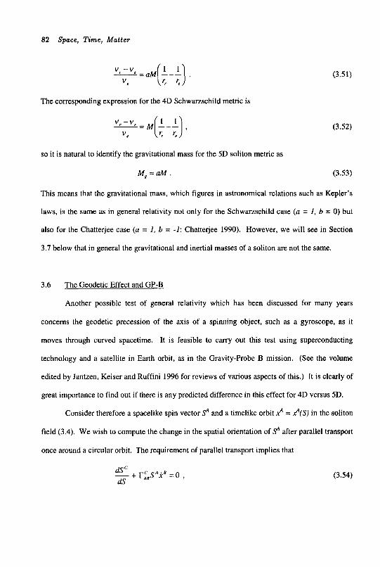
82 Space, Time, Matter
(3.51)
The corresponding expression for the 4D Schwarzschild metric is
(3.52)
so it is natural to identify the gravitational mass for the 5D soliton metric as
M, = a M . (3.53)
This means that the gravitational mass, which figures in astronomical relations such as Kepler’s
laws, is the same as in general relativity not only for the Schwarzschild case (a = I, b = 0) but
also for the Chatterjee case (a = 1, b = -1: Chatterjee 1990). However, we will see in Section
3.7 below that in general the gravitational and inertial masses of a soliton are not the same.
3.6 The Geodetic Effect and GP-B
Another possible test of general relativity which has been discussed for many years
concerns the geodetic precession of the axis of a spinning object, such as a gyroscope, as it
moves through curved spacetime. It is feasible to carry out this test using superconducting
technology and a satellite in Earth orbit, as in the Gravity-Probe B mission. (See the volume
edited by Jantzen, Keiser and Ruffini 1996 for reviews of various aspects of this.) It is clearly of
great importance to find out if there is any predicted difference in this effect for 4D versus 5D.
Consider therefore a spacelike spin vector 9 and a timelike orbit A! = $(Sj in the soliton
field (3.4). We wish to compute the change in the spatial orientation of 9 after parallel transport
once around a circular orbit. The requirement of parallel transport implies that
dS dS - + r,C,sAia = o , (3.54)
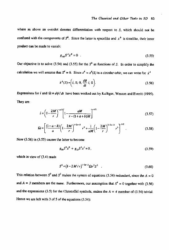
The Classical and Other Tests in 5D 83
where as above an overdot denotes differentiation with respect to S, which should not be
confused with the components of 9. Since the latter is spacelike and is is timelike, their inner
product can be made to vanish:
gAss"xB=o . (3.55)
Our objective is to solve (3.54) and (3.55) for the 9 as functions of S. In order to simplify the
calculation we will assume that 9 = 0. Since A! = &S) is a circular orbit, we can write for x A
xA(s)= i, 0, 0, - i, 0 . ( d4 dt 1 (3.56)
Expressions for i and S2 = d@/dt have been worked out by Kalligas, Wesson and Everitt (1995).
They are:
Now (3.56) in (3.55) causes the latter to become
g,so.ko + g,,S'X'=O,
(3.57)
(3.58)
(3.59)
which in view of (3.4) reads
SO=(~-~M/~)'-~"-~SZ~~S' . (3.60)
This relation between 9 and s' makes the system of equations (3.54) redundant, since the A = 0
and A = 3 members are the same. Furthermore. our assumption that .!? = 0 together with (3.56)
and the expressions (3.5) for the Christoffel symbols, makes the A = 4 member of (3.54) trivial.
Hence we are left with 3 of 5 of the equations (3.54):
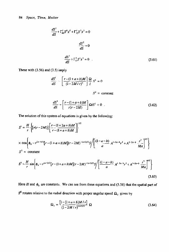
84 Space, Time, Matter
dS' dS -+ r;soio +r:,s3i3 = o
dS dS -+r:,s1i3 = o .
These with (3.56) and (3.5) imply
S' = constant
ais' = 0 . + [ r - ( l + a + b ) M dS r(r - 2M)
(3.61)
(3.62)
The solution of this system of equations is given by the following:
1r s' = H { [r(r - 2M)][ r -(1+ 2a + b ) M r - ( l + a + b ) M
S2 = constant
(3.63)
Here Hand $o are constants. We can see from these equations and (3.58) that the spatial part of
S? rotates relative to the radial direction with proper angular speed Q, given by
s [1 - (1+ a + b ) M / r] (I - 2~ / r)(n+')'Z
Qs = (3.64)
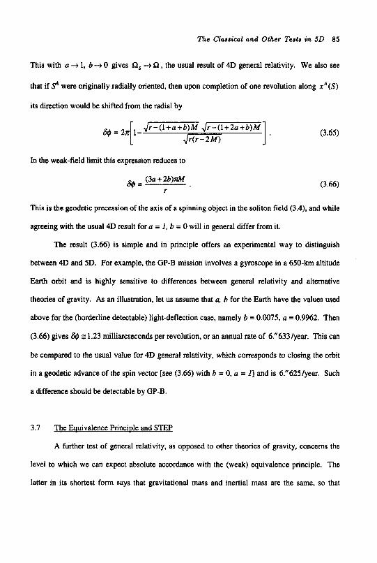
The Classical and Other Tests in 5D 85
This with a + 1, b + 0 gives Q, + 51, the usual result of 4D general relativity. We also see
that if 9 were originally radially oriented, then upon completion of one revolution along x A ( S )
its dimtion would be shifted from the radial by
I
- (1 +a + b ) M Jr - (1 + 2a + b)M .\I.(.-2~)
In the weak-field limit this expression reduces to
(30 + 2 b ) m w =
(3.65)
(3.66)
This is the geodetic precession of the axis of a spinning object in the soliton field (3.4), and while
agreeing with the usual 4D result for a = 1, b = 0 will in general differ from it.
The result (3.66) is simple and in principle offers an experimental way to distinguish
between 4D and 5D. For example, the GP-B mission involves a gyroscope in a 650-km altitude
Earth orbit and is highly sensitive to differences between general relativity and alternative
theories of gravity. As an illustration, let us assume that a, b for the Earth have the values used
above for the (borderline detectable) light-deflection case, namely b = 0.0075, a = 0.9962. Then
(3.66) gives & 5 1.23 milliarcseconds per revolution, or an annual rate of 6."633/year. This can
be compared to the usual value for 4D general relativity, which corresponds to closing the orbit
in a geodetic advance of the spin vector [see (3.66) with b = 0, a = 11 and is 6."625/year. Such
a difference should be detectable by GP-B.
3.7 The Euuivalence F'rincide and STEP
A further test of general relativity, as opposed to other theories of gravity, concerns the
level to which we can expect absolute accordance with the (weak) equivalence principle. The
latter in its shortest form says that gravitational mass and inertial mass are the same, so that
86 Space, T i m e , Matter
objects of differing natures fall at the same rate in a gravitational field (see Section 1.3). It
would not be appropriate to review here the large literatures that exist on the theoretical and
experimental sides of this issue. But we have already in Section 3.4 come upon dynamical
effects of 5D theory which appear to constitute apparent violations of the equivalence principle,
albeit at levels which are probably very low. Obviously, if there is any possibility that this
principle might not be obeyed, it should be continuously tested to even more rigorous levels.
Proposals to do this are frequent in gravitational physics. Of these, most are impractical, though
some are redeemed by imagination (e.g., Wit 1991). A practical test which promises
unprecedented accuracy involves measuring the accelerations of different test masses aboard a
satellite in Earth orbit, as in the Satellite Test of the Equivalence Principle mission. (See the
volume edited by Reinhard 1996 for reviews of various aspects of this.) In view of the extensive
literature that already exists on the topic, we will here content ourselves with a short historical
account of possible violations of the 4D equivalence principle in 5D gravity, and afterwards
make some pertinent comments about STEP and related tests.
Gross and Perry (1983) evaluated the inertial mass of a soliton by using the Landau
pseudo energy-momentum tensor, and the gravitational mass by using the metric. They found
Mi = (1 + P ) M , , so the masses are different for any finite value of the parameter p, which by
(3.3) fixes the potential associated with the fifth dimension. Only when the latter has no effect
and fl = 0 do we recover the Schwarzschild solution with Mi = M , . However, while it may
appear that (3 f 0 involves a violation of the equivalence principle, Gross and Perry argued that
the source of the discrepancy is actually just the breakdown of Birkhoff's theorem.
Deser and Soldate (1989) agreed with this analysis, though they noted that the precise
relation between mi and rng needs correcting by a factor two from the formula in Gross and
The Classical and Other Tests in 5D 87
Perry (1983). We have reworked the calculation involving the Landau tensor and confirmed that
M,=(l+P/Z)M,, as well as studying the motion of a test particle near a soliton (Billyard,
Wesson and Kalligas 1995). The important thing is that in 5D there are two different masses, a
property which inevitably makes the dynamics of Kaluza-Klein theory different from that of
Einstein theory.
Cho and Park (1991) evaluated the inertial and gravitational masses of a soliton not in 5D
but in 7D. They found them to be unequal, and at first stated that this indicated “an obvious
violation of the equivalence principle”. However, in a subsequent discussion they argued that
the extra or fifth force associated with the extended geometry is responsible for this apparent
violation, and that it should be described not as a breakdown of the equivalence principle but as a
departure from the usual (4D) law of geodesic motion.
Wesson (1996) reviewed these arguments, and by using equations of motion like those
derived in Section 3.4 above, came to the conclusion that the problem is largely one of
semantics: the relations that describe geodesic motion in 5D are not in general the same as those
which describe geodesic motion in 4D, and the extra terms from 5D look like violations of the
equivalence principle in 4D.
We will make a detailed examination of geodesic motion in 5D later, where we will find
that there are some 5D metrics where the 4D part of the 5D motion is indistinguishable from
pure 4D motion, and some metrics which imply significant differences. Here, it is worthwhile to
note that missions like STEP can in general expect two types of practical difference between 4D
and 5D physics. First, the orbit of the spacecraft as a whole will not be the same in Einstein
theory and Kaluza-Klein theory, and since the mission involves altitude-related telemetry the
difference may be detectable. Second, the accelerations of the test masses aboard the spacecraft
88 Space, Time, Matter
will not be the same if their inertial and gravitational masses differ as in Kaluza-Klein theory,
and since these can be measured to high accuracy a difference may be detectable.
3.8 Conclusion
The 4D Schwarzschild metric (3.1) is embedded in the 5D soliton metrics (3.3) and (3.4)
via a choice of parameters that effectively nullifies the influence of the fifth dimension. The
question of whether we need the latter is in principle answerable by observation and experiment.
Thus (3.18) gives the light-deflection angle, (3.25) gives the radar-ranging time delay, (3.31)
gives the circular photon orbit radius, (3.38) gives the perihelion advance angle, (3.48) gives the
motion inversion radius, (3.51) gives the shift in radiation frequency, and (3.66) gives the
geodetic advance angle. Data from the solar system (Will 1992) indicate that the dimensionless
constant which measures the influence of the fifth potential is at most of order 10.’ locally.
It is of course a paradigm of current research methodology that we should embed what
we know in what we do not know, smoothly. This is really just a modern version of Occam’s
razor, and as such is laudable. But because of the finite uncertainties that attend all observations
this philosophy necessarily leads to a situation where it is difficult to validate new theory using
old data.
The way forward is to look at systems other than the solar system and to carry out new
tests in space. Specifically, we need to test the light-deflection formula by better observations of
lensed QSOs and other objects (Kochanek 1993; Gould 1994). And we need to test the
perihelion-advance formula by better observations of eclipsing binaries such as DI Herculis
(Guinan and Maloney 1985; Maloney, Guinan and Boyd 1989), binary pulsars (Haugan 1985;
Taylor and Weisberg 1989) and possible pulsars with planetary comparisons (Wolszczan and
Frail 1992; Thorsett and Phillips 1992). Also, we need to test the geodetic-precession formula
The Classical and Other Test8 in 5 0 89
by carrying out missions like GP-B, and we need to test the equality of gravitational and inertial
mass by carrying out missions like STEP.
References (ChaDter 3)
Adler, R., Bazin. M. Schiffer, M. 1975, Introduction to General Relativity (2nd ed., McGraw-
Hill, New York).
Billyard, A., Wesson, P.S., Kalligas, D. 1995, Int. J. Mod. Phys. D4.639.
Chatterjee, S. 1990, Astron. Astrophys. 230, 1.
Cho, Y.M., Park, D.H. 1991, Gen. Rel. Grav. 23,741.
Davidson, D., Owen, D. 1985, Phys. Lett. B 155,247.
Deser, S., Soldate, M. 1989, Nucl. Phys. €3 311,739.
Gould, A. 1994, Astrophys. J. 435,573.
Gross, D.J., Perry, M.J. 1983, Nucl. Phys. B 226.29.
Guinan, E.F., Maloney, F.P. 1985, Astron. J. 90, 1519.
Haugan, M.P. 1985. Astrophys. J. 296.1.
Jantzen, R.T.. Keiser, G.M., Ruffini, R. (eds.) 1996, Proc. 7th Marcel Grossman Meeting (World
Scientific, Singapore).
Kalligas, D., Wesson, P.S., Eventt, C.W.P. 1995, Astrophys. J. 439,548.
Kochanek, C.S. 1993, Astrophys. J. 419, 12.
Lim, P., Overduin, J.M., Wesson, P.S. 1995, J. Math. Phys. 3,6907.
Maloney, F.P., Guinan, E.F., Boyd, P.T. 1989, Astron. J. 98, 1800.
Reinhard, R. (ed.) 1996, STEP: Testing the Equivalence Principle in Space (European Space
Agency, WPP-115).
Taylor, J.H., Weisberg, J.M. 1989, Astrophys. J. 345,434.
90 Space, Time, Matter
Thorsett, S.E., Phillips, J.A. 1992, Astrophys. J. 387, L69.
Wesson, P.S. 1996, STEP: Testing the Equivalence Principle in Space (European Space
Agency, WPP-115), 566.
Will, C.M. 1992, Int. J. Mod. Phys. D 1, 13.
Wit, P.S. 1991, Gravitation: A Banff Summer Institute (eds. Mann, R., Wesson, P.S., World
Scientific, Singapore), 638.
Wolszczan, A., Frail, D.A. 1992, Nature 355, 145.
4. COSMOLOGY AND ASTROPHYSICS IN 5D
“Was there really a big bang?’ (Sir Martin Rees, Toronto, 1997)
4.1 Introduction
In Chapter 2, we learned that cosmological matter with uniform density and pressure can
be regarded as induced in 4D from SD, and gave a general prescription for neutral matter
wherein 4D physical quantities are derived from 5D geometrical quantities. There is now a
considerable literature on induced-matter theory. In this chapter, however, we will concentrate
on solutions of cosmological and astrophysical importance. We will take a closer look at the
‘standard’ cosmological model, and then examine a model for spherically-symmetric clouds of
matter which has general application to astrophysical systems (e.g. clusters of galaxies). These
models basically agree with cosmological and astrophysical data because they smoothly embed
4D solutions in 5D solutions. The induced-matter theory goes further, though, and in the last
half of this chapter we will look at new types of solutions of cosmological relevance. These
include a solution which describes waves in a de Sitter vacuum and has implications for
inflation, and a time-dependent version of the static soliton examined before which may help
explain how these objects formed. We will also look briefly at systems with axial and
cylindrical symmetry, which while of mainly mathematical interest have implications for the
(none) inevitability of big-bang singularities. Lastly, we will present a shell-like solution, which
while derived for use in particle physics may also be used as a model for the cellular structure
which seems to be a common feature of cosmological surveys.
91
92 Spece, Time, Matter
4.2 The Standard Cosmological Model
This was presented in Section 2.2 as the induced-matter version of a 5D solution to RAB =
0 derived originally by Ponce de Leon (1988). In the present section we will present it in a new
way, using results from coordinate transformations and the geodesic equation (Mashhoon, Liu
and Wesson 1994; Wesson 1994a; Wesson and Liu 1995). After some algebraic work, we will
make contact with observations via the subjects of dark matter, the 3K microwave background
and a possible time-variation of particle masses.
Any solution of 5D RAE = 0 can be written as a solution of 4D G, = 8a T, with an
effective or induced energy-momentum tensor, given by (2.53) as:
Here as before, a),, = a/ a x a , a semicolon denotes the 4D covariant derivative, and an asterisk
means The form of (4.1) depends on a gauge or coordinate choice wherein the 5D
interval is written dS2 = g,,drAdxB, with a 5D metric tensor
g,, = (g,, g,, = 0, g, = &*, &=k 1). However, while this gauge suppresses overtly
electromagnetic effects, the results it leads to are general in the sense that as long as we allow
gAB to be x4-dependent we have only used 4 of the 5 available coordinate degrees of freedom
(see Section 2.5). This leaves I over, which we will use below in a way indicated by the history
of physical measurements (see Section 1.2). We will use (4.1) above to derive all relevant
properties of matter for the 5D solutions presented below.
For cosmology, let us start buddhistically with featureless, flat 5D space:
Cosmology and Astrophysics in 5 0 93
ds2 = dt2 - dr2 - r2dSZ2 - d12 . (4.2)
Here the coordinates of spacetime are the time (t) and spherical polars
(r,8,q4:dQa r=d02+sin28dt$2), and the extra coordinate is x4 = 1 . Let us now change
coordinates to
T = t
Then (4.2) becomes
d s 2 = f l 2 - L Z [ - dR2 +R2dS2 ' ] -dL2 . (1 - R2)
(4.3)
(4.4)
If we now put this into (4.1) and take the matter to be a perfect fluid (To = p , I;' =- p) , we find
that its density and pressure are given by
(4.5)
The equation of state here is typical of situations in 4D where the gravitational or Tolman-
Whittaker mass is zero (see Section 2.4). Since matter with this equation of state does not
disturb other objects gravitationally, it has been suggested as relevant to cosmic strings (Gott and
Rees 1987; Kolb 1989), zero-point fields (Wesson 1991, 1992), and extreme sources for the
Reissner-Nordstrom metric (Ponce de Leon 1993). However, it is always possible to split the
density and pressure up into parts that are due to matter and parts that are due to vacuum, where
the latter are related to the cosmological constant via p, = A I8n = -p, . Thus if we write
p = p, + p, andp = pm + pv in (4.5), introduce A and set pm = 0, we obtain
1 8 ~ = - - p + 3 p = O . 3 8np = - L2 L2
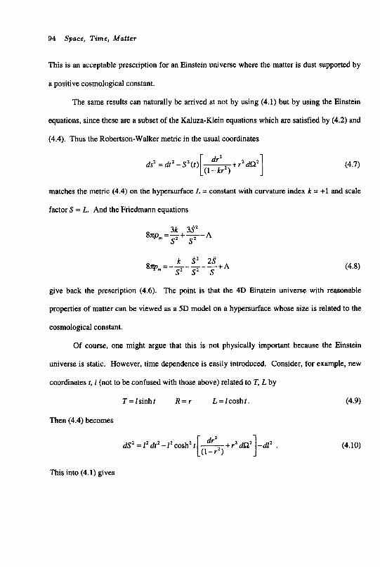
94 Space, Time, Matter
This is an acceptable prescription for an Einstein universe where the matter is dust supported by
a positive cosmological constant.
The same results can naturally be arrived at not by using (4.1) but by using the Einstein
equations, since these are a subset of the Kaluza-Klein equations which are satisfied by (4.2) and
(4.4). Thus the Robertson-Walker metric in the usual coordinates
dS2 =dt2-Sz(t) [ - dr2 +r2dQ2 (1- kr2) (4.7)
matches the metric (4.4) on the hypersurface L = constant with curvature index k = +1 and scale
factor S = L. And the Friedmann equations
(4.8)
give back the prescription (4.6). The point is that the 4D Einstein universe with reasonable
properties of matter can be viewed as a 5D model on a hypersurface whose size is related to the
cosmological constant.
Of course, one might argue that this is not physically important because the Einstein
universe is static. However, time dependence is easily introduced. Consider, for example, new
coordinates r, f (not to be confused with those above) related to T, L by
T=l s inh t R = r L= lcosh t . (4.9)
Then (4.4) becomes
dS2 =12dt2-lZcosh2t ~ i r 2 d Q z -d12 . (1-r’) 1 (4.10)
This into (4.1) gives
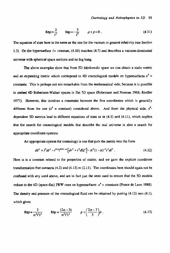
Cosmology and Astrophysics in 5 0 95
(4.11)
The equation of state here is the same as the one for the vacuum in general relativity (see Section
1.3). On the hypersurface I = constant, (4.10) matches (4.7) and describes a vacuum-dominated
universe with spherical space sections and no big bang.
3 3 l 2
a 7 p S " 8np=-- p + p = o .
The above examples show that from 5D Minkowski space we can obtain a static metric
and an expanding metric which correspond to 4D cosmological models on hypersurfaces x' =
constants. This is perhaps not too remarkable from the mathematical side, because it is possible
to embed 4D Robertson-Walker spaces in flat 5D space (Robertson and Noonan 1968; Rindler
1977). However, this involves a constraint between the five coordinates which is generally
different from the one (x' = constant) considered above. And from the physical side, x'-
dependent 5D metrics lead to different equations of state as in (4.5) and (4.11). which implies
that the search for cosmological models that describe the real universe is also a search for
appropriate coordinate systems.
An appropriate system for cosmology is one that puts the metric into the form
dsZ = 12dt2 -t21a121(1-a) [d.' + r2dSZZ] - d ( 1 - a)-2t2dIZ . (4.12)
Here a is a constant related to the properties of matter, and we gave the explicit coordinate
transformation that connects (4.2) and (4.12) in (2.1 1). The coordinates here should again not be
confused with any used above, and are in fact just the ones used to ensure that the 5D models
reduce to the 4D (space-flat) PRW ones on hypersurfaces x4 = constants (Ponce de Leon 1988).
The density and pressure of the cosmological fluid can be obtained by putting (4.12) into (4.1),
which gives
(4.13)
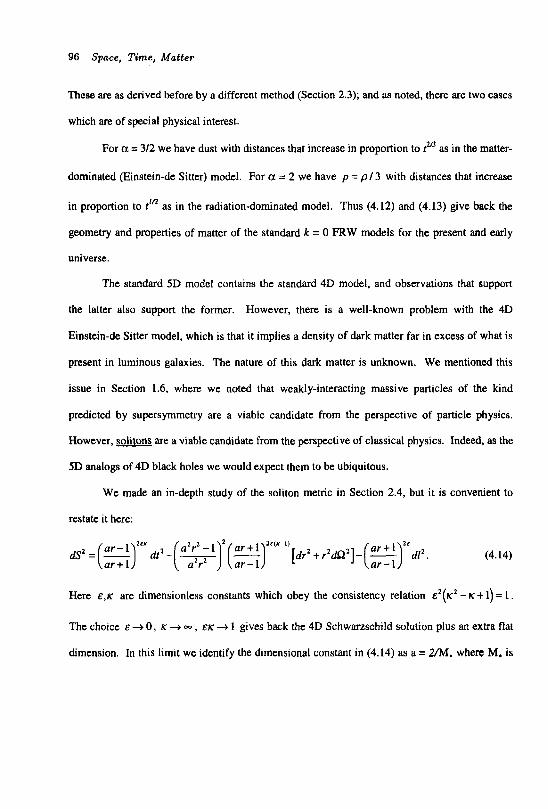
96 Space, Time, Matter
These are as derived before by a different method (Section 2.3); and as noted, there are two cases
which are of special physical interest.
For a = 3/2 we have dust with distances that increase in proportion to p3 as in the matter-
dominated (Einstein-de Sitter) model. For a = 2 we have p = p / 3 with distances that increase
in proportion to tlR as in the radiation-dominated model. Thus (4.12) and (4.13) give back the
geometry and properties of matter of the standard k = 0 FXW models for the present and early
universe.
The standard 5D model contains the standard 4D model, and observations that support
the latter also support the former. However, there is a well-known problem with the 4D
Einstein-de Sitter model, which is that it implies a density of dark matter far in excess of what is
present in luminous galaxies. The nature of this dark matter is unknown. We mentioned this
issue in Section 1.6, where we noted that weakly-interacting massive particles of the kind
predicted by supersymmetry are a viable candidate from the perspective of particle physics.
However, solitons are a viable candidate from the perspective of classical physics. Indeed, as the
5D analogs of 4D black holes we would expect them to be ubiquitous.
We made an in-depth study of the soliton metric in Section 2.4, but it is convenient to
restate it here:
(4.14)
Here &,K are dimensionless constants which obey the consistency relation &'(K' - K + 1) = I .
The choice E + 0, K + - , EK -+ 1 gives back the 4D Schwarzschild solution plus an extra flat
dimension. In this limit we identify the dimensional constant in (4.14) as a = 2/M. where M. is
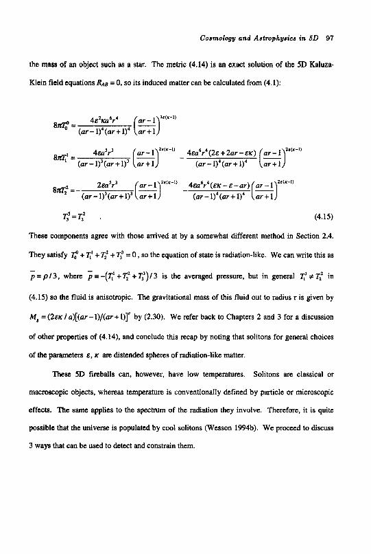
Coamology and Aatrophyaica in 5 0 97
the mass of an object such as a star. The metric (4.14) is an exact solution of the 5D Kaluza-
Klein field equations RAE = 0, so its induced matter can be calculated from (4.1):
g=q' . (4.15)
These components agree with those anived at by a somewhat different method in Section 2.4.
They satisfy +I;' t T,' +I;' = 0 , so the equation of state is radiation-like. We can write this as
- p = p / 3, where i -(I;' + T,' t I;')/ 3 is the averaged pressure.. but in general I;' # T," in
(4.15) so the fluid is anisotropic. The gravitational mass of this fluid out to radius r is given by
M, = (2.5~ / a)[(ar - l)/(ar + 1)r by (2.30). We refer back to Chapters 2 and 3 for a discussion
of other properties of (4.14), and conclude this recap by noting that solitons for general choices
of the parameters E , K are distended spheres of radiation-like matter.
These 5D fireballs can, however, have low temperatures. Solitons are classical or
macmcopic objects, whereas temperature is conventionally defined by particle or microscopic
effects. The same applies to the spectrum of the radiation they involve. Therefore, it is quite
possible that the universe is populated by cool solitons (Wesson 1994b). We proceed to discuss
3 ways that can be used to detect and constrain them.
98 Space, T i m e , Matter
Background radiation can be significantly affected by solitons, because by (4.15) they
have extended matter. The length scale of the distribution is set by the dimensional constant a in
(4.14), which while it is related to the Schwarzschild mass in the 4D limit should be regarded as
a geometrical parameter of more generality in the 5D case. For r >> 1 I a, p~ E*K / 2m2r4 and
M, P 2 E K / a . Combining these expressions and restoring conventional dimensions gives the
density at large distances as
G M , ~ 8m2Kr4 '
pr - (4.16)
The parameter K here is free to choose physically, but a particularly convenient choice for the
purpose of illustration is K = 1. Let us take this and assume that solitons of mass M. are
uniformly distributed with mean density p , so that the average separation is of order
d = (M. / Z)'''. Then the energy density of the nearest soliton is given by (4.16) with r = d , and
is
(4.17)
This is actually sufficient to work out the expected energy density of a collection of solitons,
because in the uniform case the volume of space varies as r3 while the energy density of a given
soliton varies as r4, so the nearest one dominates. The equation of state of the matter of a
soliton is radiation-like as we saw above, so we shall assume that the matter is indeed photons.
Unfortunately, we do not have spectral information on these (which would come from a detailed
model), and so are obliged to proceed bolometrically. However, we can obtain an interesting
result by considering a cosmological medium of solitons and comparing with the cosmic
microwave background. Thus, let us consider a medium consisting of solitons with galactic
Cosmology and Astrophysics in 5 0 99
mass M. = 5 x 10” Ma and mean density = 1 x lo-% g cm”. Then (4.17) shows that the nearest
soliton would produce a contribution which compared to that of the uniform background would
be of order 10”. Since the Cosmic Background Explorer (COBE) and other instruments have
restricted anomalous contributions to this order, we infer that if the dark matter consists of
solitons then they are probably less massive than galaxies.
Galactic morphology can be used to bolster this inference. It is well known that objects
consisting of conventional dark matter must be less than of order 10’ M, if the ones near to
regular galaxies are not to affect the shapes of the latter through tidal interactions. A similar
argument can be applied to solitons. However, it is not so straightforward. In our preceding
discussion of background radiation, we were concerned with one soliton and chose a convenient
value of K for it (K = 1, which by the consistency relation implies E = 1 also). For interacting
populations of galaxies and solitons, however, the latter would presumably have a range of
values of E and K. And some values of these parameters can make the effective masses of
solitons quite small. For example, K = 0.1 implies that E = 1.05, so for r >> i/u we have M, =
0.105(2/a) = 0.105 M. and an effective mass only one-tenth of what it would be conventionally.
(The extreme case EK + 0 corresponds to an object with zero gravitational mass which is the
original Gross and Perry soliton.) We infer that while it is certainly possible, it will take some
care to constrain solitons via their effects on the morphologies of regular galaxies.
Gravitational lensing is a mom clear-cut effect. Let us assume that a light ray originates
in a distant source, suffers a slight deflection 8 as it passes near a soliton, and anives at us. This
problem was considered in detail in Chapter 3. There we introduced a quasi-Schwarzschild
coordinate r‘ = r(l+ 1 I ar)’ more suited to observations than the isotropic r of (4.14). We also
100 Space, Time, Matter
introduced 3 constants of the motion, which we here relabel k,, k2, k3 and use to define a new
constant d 2 (2& - ~ - 2 ) k : +(2&-& +2)k:. Then the deflection angle with conventional
dimensions restored is given by
4GM. 2GM.dr2, c r,, c Z k t '
s=- 2 , + (4.18)
Here rAn is the minimum distance of passage of light to the soliton (or impact parameter), and
the first term is the usual one found in 4D theory. The second term is special to 5D theory, and
is in principle measurable. It is possible to use the lensing of light from QSOs to look for
extragalactic solitons and microlensing to look for solitons associated with the Galaxy.
The preceding discussion on dark matter touched at several places on background
radiation. This includes the integrated radiation from stars in galaxies at various wavelengths
and the contribution from dark-matter particles which are unstable to decay. (It is generally
acknowledged that constraints on the so-called extragalactic background light are an effective
way to restrict dark-matter particles). However, it also includes the 3K background radiation,
whose spectrum has been established by COBE and other instruments to be accurately black
body, and is commonly regarded as having been produced by the big bang. Also,
nucleosynthesis of the elements is supposed to have occurred in the fireball that followed the big
bang. However, there is a problem of logic involved here. This has been realized by a few
workers (notably Dicke, Dirac, and Hoyle and Narlikar: see Wesson 1978 for a review). But
while it is not generally appreciated, i t is deadly.
In 4D, the FRW solutions with metric (4.7) are typically written in comoving coordinates.
That is, the solutions are derived under the assumption (which is mathematically valid) that there
is a choice of coordinates where dZ3 = 0 for the 3 spatial components of the 4-velocity

Cosmology and Astrophysics in 5 0 101
ua I dx" / ds . In this frame, galaxies do not move and always retain the same separations from
each other. So where (in a physical sense) are the 3K background and nucieosynthesis supposed
to fit in? The naive response is that the comoving frame is not 'real', and that in another frame
the galaxies are 'really' moving apart in accordance with Hubble's law, and that tun backwards
in time the universe in this non-comoving frame would at early times produce the extreme
conditions necessary to account for the generation of the background radiation and the elements.
Such a rationalization has no justification in mathematics or logic. This because, according to
4D general relativity and the principle of (coordinate) covariance on which its equations are
based, the comoving frame is just as valid as the non-comoving frame. A little thought shows
that this conundrum has a simple solution: 4D algebraic covariance is incomdete with regard to
physical processes.
In 5D, this problem can in principle be solved (Wesson and Liu 1995). The fulcrum of
the argument involves the physical meaning of the coordinate x4 = 1 used in the metric of the
standard cosmological model (4.12). This metric has comoving spatial coordinates and on the
hypersurface x' = constant has an interval given by dS = I&. This should be consistent with 4D
particle dynamics, whose corresponding interval or action is defined by ds = mdt. Clearly in this
case at least, x' = 1 has the physical interpretation of particle rest mass. This agrees with the
algebraic possibility of geometrizing mass (Chapter l), and with the fact that in general x'-
independent metrics describe fluids consisting of photons whereas x'-dependent metrics describe
fluids consisting of massive particles (Chapter 2). Indeed, there is a form for the 5D metric
which because of the simplification for particle motion which it implies is called canonical
(Mashhoon, Liu and Wesson 1994); and it can be shown that if we wish to give a geometric
description of the rest mass m of a particle in 4D Einstein theory, then for canonical metrics in
102 Space, Time, Matter
5D Kaluza-Klein theory the appropriate identification is 1 = m (Chapter 7). There is a
surprisingly extended history of attempts to relate the extra coordinate of 5D relativity to mass,
and what we have stated here is only designed to open a prospect to a solution of the covariance
problem outlined in the previous paragraph. That this is possible is clear if we recall that we
have 1 coordinate degree of freedom left over to use as we wish. Depending on what we choose,
we can have a frame where x4 and masses are constants, or a frame where x4 and masses are
variable. The former is of course the one which has been used in physics historically, but the
latter is also acceptable and leads to new insights cosmologically.
To see what is involved here, let us consider the 5D geodesic equation
dUC dS
-+T,C,UAUB = 0 (4.19)
Here the 5-velocities are related to the 4-velocities via UA = d r A Ids=
(dr" I &)(A/ dS) = u"(ds I dS) when A = a = 0,123. To get the other component,
U' = dx4 / dS, we need the following 5D Christoffel symbols for metric (4.12):
(4.20)
Then expanding (4.19) shows that its spatial components are satisfied with comoving coordinates
of the conventional type (U' = Uz = v-' = U), while the zeroth and fourth components yield
(4.21)
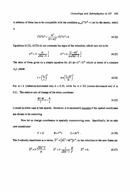
Cosmology and Aatrophysics in 5D 103
A solution of these has to be compatible with the condition g,UAUn = 1 set by the metric, which
is
Equations (4.21), (4.22) do not constrain the signs of the velocities, which turn out to be
(4.22)
(4.23)
The ratio of these gives us a simple equation for dl I dt = U4 / UQ which in terms of a constant
0 0 ) Yields
(4.24)
For a = 2 (radiation-dominated era) A = 0.25, while for a = 312 (matter-dominated era) A P
0.1 1. The relative rate of change of the extra coordinate
d l l d t A 1 I
-=-- (4.25)
is small in either case at late epochs. However, it is necessarily nonzero if the spatial coordinates
arc chosen to be comoving.
Now let us change coordinates to spatially noncomoving ones. Specifically, let us take
new coordinates
T = tl R=t"ur L=AtAl . (4.26)
I &')Un, so the velocities in the new frame are The 5-velocity transforms as a vector, Ti" =
(4.27)
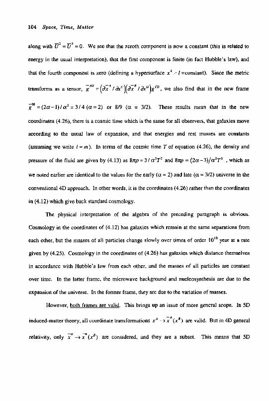
104 Space, Time, Matter
along with i?' = i?' = 0. We see that the zeroth component is now a constant (this is related to
energy in the usual interpretation), that the first component is finite (in fact Hubble's law), and
that the fourth component is zero (defining a hypersurface x4 = 1 =constant). Since the metric
transforms as a tensor, gA6 = ( d i A /&')(d? / A D ) g C D , we also find that in the new frame
-w g = (2a-1)/ a' = 3 / 4 (a = 2) or 8/9 (a = 3/2). These results mean that in the new
coordinates (4.26), there is a cosmic time which is the same for all observers, that galaxies move
according to the usual law of expansion, and that energies and rest masses are constants
(assuming we write 1 = m). In terms of the cosmic time T of equation (4.26), the density and
pressure of the fluid are given by (4.13) as 8np = 3/a2T2 and 87p = (2a-3)/aZT2 , which as
we noted earlier are identical to the values for the early (a = 2) and late (a = 312) universe in the
conventional 4D approach. In other words, it is the coordinates (4.26) rather than the coordinates
in (4.12) which give back standard cosmology.
The physical interpretation of the algebra of the preceding paragraph is obvious.
Cosmology in the coordinates of (4.12) has galaxies which remain at the same separations from
each other, but the masses of all particles change slowly over times of order 10" year at a rate
given by (4.25). Cosmology in the coordinates of (4.26) has galaxies which distance themselves
in accordance with Hubble's law from each other, and the masses of all particles are constant
over time. In the latter frame, the microwave background and nucleosynthesis are due to the
expansion of the universe. In the former frame, they are due to the variation of masses.
However, both frames are valid. This brings up an issue of more general scope. In 5D
induced-matter theory, all coordinate transformations x A + ; " (x" ) are valid. But in 4D general
relativity, only x" x"(xa) are considered, and they are a subset. This means that 5D

C O S f f l O l O g y and Astrophysics in 5 0 105
coordinate transformations can change 4D physics. [A particular example of this is that a
coordinate transformation takes us from a universe with metric (4.2) that is empty to a universe
with metric (4.12) that has matter.] For the case of cosmology, we have shown above that the
conventional interpretation of observations implies a choice of coordinates where masses are
constant, which of course agrees with the widespread view that they provide a system of
standards (see Chapter 1). However, it is not really clear if this is the system of coordinates
which is being used in astrophysics in Dractice; and the system with time-variable masses is
actually very close. Thus consider (4.25) for the rate of change of the extra coordinate in the
present (dust) universe. It predicts m/m =-O.ll/t0 (where an overdot denotes the rate of
change and to is the present epoch). For to = 18 x lo9 year we have h / m ~ - 6 x lo-’* yr-’.
This is marginally consistent with ranging data from the Viking space probe to Mars (where the
errors are reported as f 4 ~ 1 0 ” ~ yr” and f 10 x 10” yi’) and quite consistent with timing data
for the binary pulsar 1913 + 16 (where the errors are reported as f 11 x lo-’’ yr-’: see Will
1991). In the context of 5D theory, these data should be viewed as meaning that we are close to
deciding by observation what system of coordinates is being used in astrophysics.
4.3 Sohericallv-Svmrnetric AstroDhvsical Svstems
It is common practice to model astrophysical systems which are not grossly asymmetric
as spherical clouds of matter with inhomogeneous density profiles. For example, rich or Abell
clusters of galaxies can be modeled as static, isothermal spheres with power-law density profiles.
In this section, we will study a general metric and then give a static solution with inverse-square
isothermal matter (Billyard and Wesson 1996a). The latter is the 5D analog of a well-known 4D

106 Space, Tame, Matter
solution (Henriksen and Wesson 1978). There are presumably many solutions of the 5D
equations we will present below which contain known 4D solutions.
We take a spherically-symmetric metric in the form
dSz = eVdt2 - eAdr2 - R2dQ2 + &e"dlz . (4.28)
Here the metric coefficients v , A, R , p can depend in general on the time t , radius r and the
extra coordinate I . The nonzero components of RAB for (4.28) are
R l R R , . --+---(v-d-b) R2 R 2R
1 -A' i p') -+ ER2e-' .. . 1
J R 2 R R " ' RZ R 2R --+ -+-(v+ A - p )
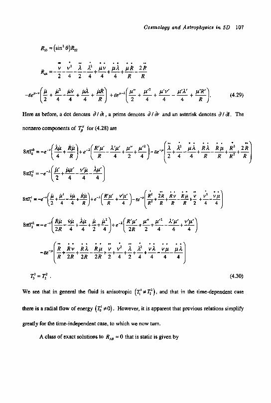
Cosmology and Astrophysics in 5D 107
R,, = (sin2 e)h2
. . I , , . .. R - ____-___ +-+-+--- v v2 i i' pv pjl p R 2 R
2 4 2 4 4 4 R R u -
Here as before, a dot denotes d I dt , a prime denotes d l dr and an asterisk denotes d I d. The
nonzero components of qa for (4.28) are
R Rv R A R p v v2 ,I A' V A v p pA R 2 R 2 R 2 R 2 4 2 4 4 4 4 -+-+---+-+-+-+-+----- n . . . . . . . . * . . a . . . .
1;'= q= . (4.30)
We see that in general the fluid is anisotropic (T,'#q'), and that in the time-dependent case
there is a radial flow of energy (&I #O) . However, it is apparent that previous relations simplify
greatly for the time-independent case, to which we now turn.
A class of exact solutions to R,, = 0 that is static is given by
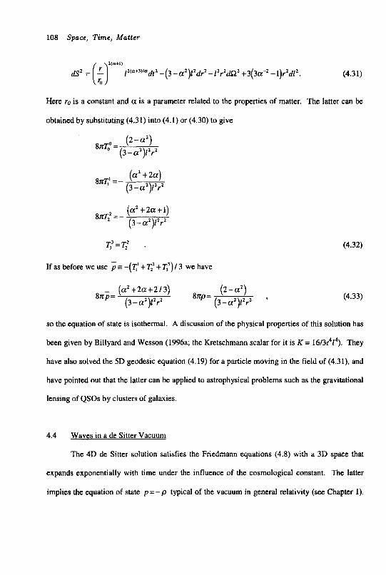
108 Space, Time, Matter
Here ro is a constant and a is a parameter related to the properties of matter. The latter can be
obtained by substituting (4.31) into (4.1) or (4.30) to give
(2 - aZ) sm: = (3-aZ)iZrZ
(aZ + 201) ( 3 - ( 1 1 ~ ) ~ ~ r ~
8 G ' = -
(aZ+2a+i) (3 - a2)12r2
am; = -
q3=q2 .
If as before we use = -( T,' + T,' + q') / ~ we have
- ( a 2 + 2 a + 2 / 3 ) (2 -a') 8np = 8np=
(3-a2)12r2 (3-aZ)zZrZ '
(4.32)
(4.33)
so the equation of state is isothermal. A discussion of the physical properties of this solution has
been given by Billyard and Wesson (1996a; the Kretschmann scalar for it is K = 16/3r414). They
have also solved the 5D geodesic equation (4.19) for a particle moving in the field of (4.3 I), and
have pointed out that the latter can be applied to astrophysical problems such as the gravitational
lensing of QSOs by clusters of galaxies.
4.4 Waves in a de Sitter Vacuum
The 4D de Sitter solution satisfies the Friedmann equations (4.8) with a 3D space that
expands exponentially with time under the influence of the cosmological constant. The latter
implies the equation of state p = - p typical of the vacuum in general relativity (see Chapter 1).
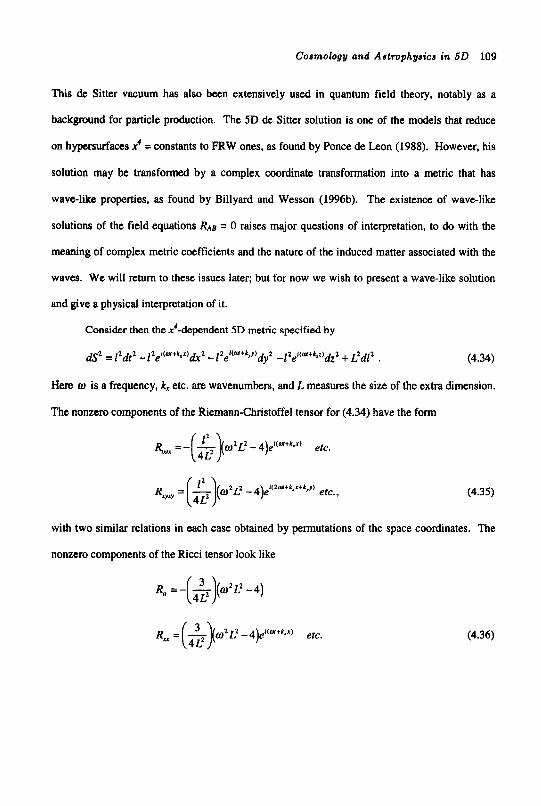
Cosmology ond Astrophysics in 5 0 109
This de Sitter vacuum has also been extensively used in quantum field theory, notably as a
background for particle production. The 5D de Sitter solution is one of the models that reduce
on hypersurfaces x' = constants to FRW ones, as found by Ponce de Leon (1988). However, his
solution may be transformed by a complex coordinate transformation into a metric that has
wave-like properties, as found by Billyard and Wesson (1996b). The existence of wave-like
solutions of the field equations RAB = 0 raises major questions of interpretation, to do with the
meaning of complex metric coefficients and the nature of the induced matter associated with the
waves. We will return to these issues later; but for now we wish to present a wave-like solution
and give a physical interpretation of it.
Consider then the x4-dependent 5D metric specified by
dy2 -12ei(or*kJ)dZ2 + L2d12 . (4.34)
Here w is a frequency, k, etc. are wavenumbers, and L measures the size of the extra dimension.
The nonzero components of the Riemann-Christoffel tensor for (4.34) have the form
ds2 = iZdt2 - ~ Z e l ( 0 N + k , x ) & 2 - 1 Z e W + k , ' Y )
(4.35)
with two similar relations in each case obtained by permutations of the space coordinates. The
nonzero components of the Ricci tensor look like
(4.36)
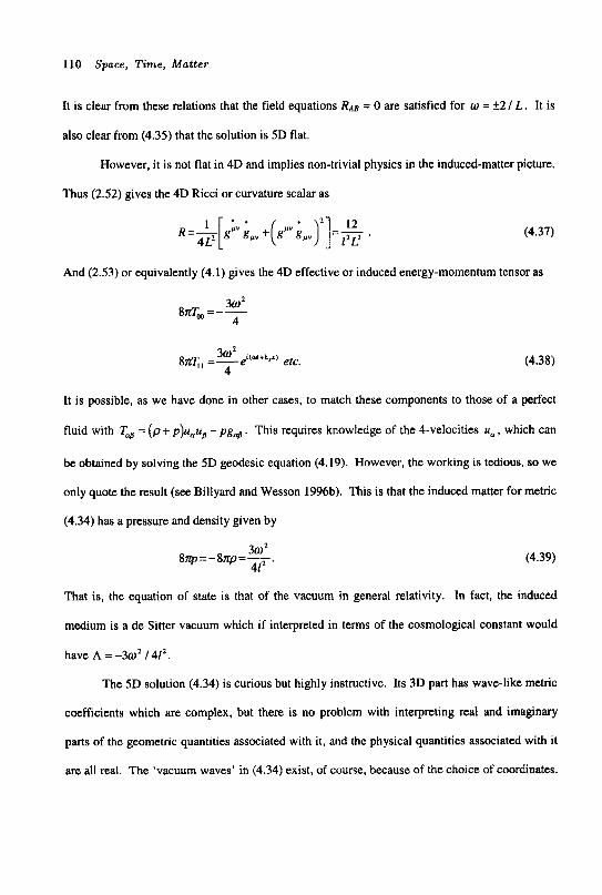
110 Space, Tame, Matter
It is clear from these relations that the field equations RAE = 0 are satisfied for o = ?2 I L . It is
also clear from (4.35) that the solution is 5D flat.
However, it is not flat in 4D and implies non-trivial physics in the induced-matter picture.
Thus (2.52) gives the 4D Ricci or curvature scalar as
(4.37)
And (2.53) or equivalently (4.1) gives the 4D effective or induced energy-momentum tensor as
(4.38)
It is possible, as we have done in other cases, to match these components to those of a perfect
fluid with T+ = (p + p)u,ua - pg+ . This requires knowledge of the 4-velocities u,, which can
be obtained by solving the 5D geodesic equation (4.19). However, the working is tedious, so we
only quote the result (see Billyard and Wesson 1996b). This is that the induced matter for metric
(4.34) has a pressure and density given by
(4.39)
That is, the equation of state is that of the vacuum in general relativity. In fact, the induced
medium is a de Sitter vacuum which if interpreted in terms of the cosmological constant would
have A=-3w2 1412.
302 8~ = -8n~p= - 412 .
The 5D solution (4.34) is curious but highly instructive. Its 3D part has wave-like metric
coefficients which are complex, but there is no problem with interpreting real and imaginary
parts of the geometric quantities associated with it, and the physical quantities associated with it
are all real. The 'vacuum waves' in (4.34) exist, of course, because of the choice of coordinates.
Cosmology and Astrophysics in 5 0 111
We can if we wish absorb the oscillatory terms in 3D by appropriate coordinate transformations,
and o can be made imaginary (which reverses the sign of the last part of the metric since
L' =41d). The result is a 5D growing-mode de Sitter solution of the type originally found by
Ponce de Leon (1988). It should, however, be noted that the standard 4D growing-mode
de Sitter solution can if one wishes also be converted to an oscillatory mode. The easiest way to
see that even 4D relativity admits vacuum waves is to look at the Friedman equations (4.8).
These are satisfied for p, = p , = 0. k = 0, S = e""' and A = -30'. Previously, such 4D
oscillatory motion would have been viewed as a mathematical quirk, but it is given legitimacy by
the 5D induced-matter approach. In either 5D or 4D, solutions of the kind we have been
discussing may be relevant to the early universe. For we can imagine a static model full of
vacuum waves with real W , which undergoes a phase change to imaginary o, resulting in an
expanding model of the inflationary type.
4.5 Time-Deoendent Solitons
The solitons studied in Section 2.4 are independent of xo = I and x' = 1 , but in the absence
of a Birkhoff-type theorem they can be generalized in both regards (see Liu, Wesson and Ponce
de Leon 1993, and Ponce de Leon and Wesson 1993, respectively). The time-dependent
extension is particularly interesting, because if static solitons exist in nature they presumably
formed by some dynarnical process. Also, time-dependent solutions which represent centrally-
condensed clouds of hot matter may be applicable to the problem of galaxy formation. Thus we
will give a class of time-dependent soliton solutions (Wesson, Liu and Lim 1993) and evaluate
their induced properties of matter.
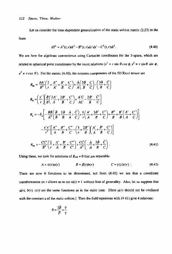
112 Space, Time, Matter
Let us consider the time-dependent generalization of the static soliton metric (2.23) in the
form
dSz = AZ(t,r)dtz - B2(t,r)dr'dx' -CZ(t ,r)dlZ. (4.40)
We are here for algebraic convenience using Cartesian coordinates for the 3-space, which are
related to spherical polar coordinates by the usual relations (x' = r sin 8 cos q5, 2 = r sin0 sin 4,
2 = r cos 0). For the metric (4.40), the nonzero components of the 5D Ricci tensor are
+- A ( 3 B -+- C)-[y -+- E) A B C
BE B 2B A C 1 A' 3B' C' B' A' C' ' '[ -- A ' ( B -+---+- B A C ) +- r ( A -+ 7+F).%+%(7+7)]
(4.41)
Using these, we look for solutions of RAB = 0 that are separable:
A = a(r)a(r) B = B(r)b(r) C = y ( t ) c ( r ) . (4.42)
There are now 6 functions to be determined, but from (4.40) we see that a coordinate
transformation on r allows us to set a(t) = 1 without loss of generality. Also, let us suppose that
a(r), b(r), c(r) are the same functions as in the static case. [Here a(r) should not be confused
with the constant a of the static soliton.] Then the field equations with (4.41) give 4 relations:
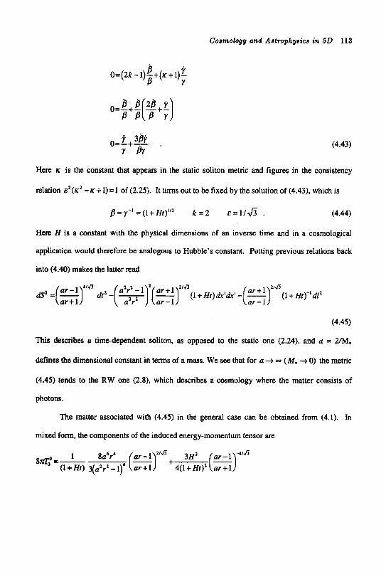
Cosmology and Astrophysics an 5 0 113
0=(2k - 1)-+(K a + 1)- Y B Y
y 3gy Y PY
o=-+- . (4.43)
Here K is the constant that appears in the static soliton metric and figures in the consistency
relation E'(K' - K + 1) = 1 of (2.25). It turns out to be fixed by the solution of (4.431, which is
B = y-' = (1+ Ht)"' k = 2 & = l I f i . (4.44)
Here H is a constant with the physical dimensions of an inverse time and in a cosmological
application would therefore be analogous to Hubble's constant. Putting previous relations back
into (4.44)) makes the latter read
a2r*-1 ar+l ar-1
(4.45)
This describes a time-dependent soliton, as opposed to the static one (2.24), and a = 2/M.
defines the dimensional constant in terms of a mass. We see that for a + ( M . + 0) the metric
(4.45) tends to the RW one (2.8), which describes a cosmology where the matter consists of
photons.
The matter associated with (4.45) in the general case can be obtained from (4.1). In
mixed form, the components of the induced energy-momentum tensor are
8a6r4 ar-1 + 3 ~ ' (ar-1)"" - 1 8 d - 0 -- (1+Ht) 3(azr2-1)1 ( a r + l ) 4(1tHf)' ar+l

114 Space, Time, Matter
2 / 4 3 H 4a a4r4 ar-1 8fld z- ~ - (1 + Hf)' 8 (a2,' - 1)3 (Z)
2/47 1 4a'r' ar-1 8 q ' = - - (1 + H f ) JS(a2r2 - I)* (FZ)
q3=g . (4.46)
These can be compared to those for the static soliton solution (4.15) and the static spherically-
symmetric solution (4.32). We see that the fluid is anisotropic with the equation of state T' =0,
which in terms of an averaged 3D pressure is
+ 3~~ (ar+1)4/47 (4.47) - 1 8a6r4 ar-1 'IJf
(1 + Hr) 3(a2rz - 1)" (Z) p=3p=-
4(1+ Ht)' ar - 1
The first term of this expression is similar to the static case but multiplied by a time factor. The
second term represents a contribution to the density and pressure from the motion. Thus we have
a natural generalization of the properties of matter of the static soliton.
4.6 Systems with Axial and Cylindrical Symmetry
In Section 4.3 we studied spherically-symmetric solutions because they are relevant to
astrophysics. However, systems with axial and cylindrical symmetry are also relevant, notably
in 2 ways. First, axially-symmetric solutions can describe objects with spin. In this connection,
we note that there has been considerable work on 5D Ken-like solutions (Gross and Perry 1983;
Myers and Perry 1986; Clement 1986; Bruckman 1986, 1987; Frolov, Zelnikov and Bleyer 1987;
Home and Horowitz 1992; Matos 1994). However, some of these solutions are contrived and
none involves x'-dependence. Introducing the latter is difficult, and attempts to do it both
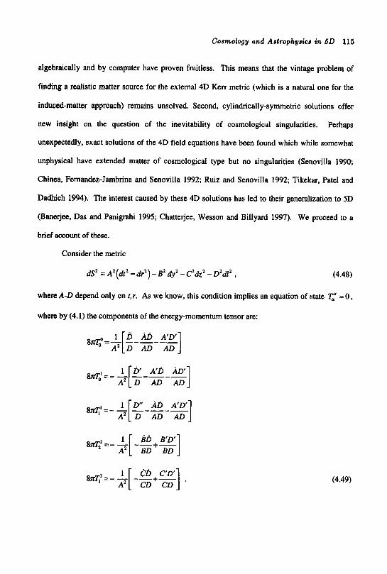
Cosmology and Astrophysics in 5 0 115
algebraically and by computer have proven fruitless. This means that the vintage problem of
finding a realistic matter source for the external 4D Kern metric (which is a natural one for the
induced-matter approach) remains unsolved. Second, cylindrically-symmetric solutions offer
new insight on the question of the inevitability of cosmological singularities. Perhaps
unexpectedly, exact solutions of the 4D field equations have been found which while somewhat
unphysical have extended matter of cosmological type but no singularities (Senovilla 1990;
Chinea, Fernandez-Jambrina and Senovilla 1992; Ruiz and Senovilla 1992; Tikekar, Pate1 and
Dadhich 1994). The interest caused by these 4D solutions has led to their generalization to 5D
(Baneqee, Das and Panigrahi 1995; Chattejee, Wesson and Billyard 1997). We proceed to a
brief account of these.
Consider the metric
dS2 =A'(dt' -dr')- B'dy2 -C2dz'- D'dl' , (4.48)
where A-D depend only on t,r. As we know, this condition implies an equation of state TE = 0 ,
where by (4.1) the components of the energy-momentum tensor are:
(4.49)
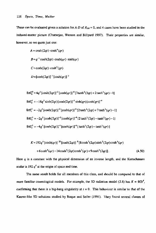
116 Space, Time, Matter
These can be evaluated given a solution for A-D of RAE = 0, and 4 cases have been studied in the
induced-matter picture (Chatterjee, Wesson and Billyard 1997). Their properties are similar,
however, so we quote just one:
A = cosh(2qt).cosh4(qr)
B=q" cosh(2qr) .cosh(qr) .sinh(qr)
C = cosh(2qf). cosh'(qr)
D =[cosh(2qt)]-' [cosh(qr)]-'
S f l ; =4q2 [cosh(2qr)]-' [cosh(qr)]-' [3tanhZ(2qr)+2 tanh'(qr)- 11
S f l , = -16q' ~inh(2qr)[cosh(2qt)]-~ sinh(qr)[c~sh(qr)]-~
S f l : = -2q' [cosh(2qt)]-' [cosh(qr)]-' [2tanhZ(2qr)+7 tanhZ(qr)-11
S f l ; = -2q'[~osh(2qr)]-'[cosh(qr)]-~ [2 tanh'(2qt)- tanh'(qr)-1]
8 f l : = -49' [cosh(2qt)]-' [cosh(qr)]-' [ tanh'(2qr)- tanh'(qr)]
K = 192q4 [c~sh(qr)]-~ [cosh(2qr)]-' [8cosh2(2qr)sinh2(2qr)cosh4(qr)
+ 6cosh4(qr) - 14cosh4(2qt)cosh2(qr) +9cosh4(2qr)J. (4.50)
Here q is a constant with the physical dimension of an inverse length, and the Kretschmann
scalar is 192 4' at the origin of space and time.
The same result holds for all members of this class, and should be compared to that of
more familiar cosmological models. For example, the 5D radiation model (2.8) has K = 9L2r4,
confirming that there is a big-bang singularity at r = 0. This behaviour is similar to that of the
Kasner-like 5D solutions studied by Roque and Seller (1991). They found several classes of
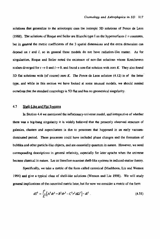
Cosmology and Astrophysics in 5 0 117
solutions that generalize to the anisotropic case the isotropic 5D solutions of Ponce de Leon
(1988). The solutions of Roque and Seiler are Bianchi type I on the hypersurfaces 1 = constants,
but in general the metric coefficients of the 3 spatial dimensions and the extra dimension can
depend on t and 1 , so in general these models do not have radiation-like matter. As for
singularities, Roque and Seiler noted the existence of non-flat solutions whose Kretchmann
scalars diverged for t + 0 and I + 0, and found a non-flat solution with zero K. They also found
5D flat solutions with (of course) zero K. The Ponce de k o n solution (4.12) is of the latter
type, and while in this section we have looked at some unusual models. we should remind
ourselves that the standard cosmology is 5D flat and has no geometrical singularity.
4.7 she 11-Like and Flat Systems
In Section 4.4 we mentioned the inflationary-universe model, and irrespective of whether
there was a big-bang singularity it is widely believed that the presently observed structure of
galaxies, clusters and superclusters is due to processes that happened in an early vacuum-
dominated period. These processes could have included phase changes and the formation of
bubbles and other particle-like objects, and are essentially quantum in nature. However, we need
corresponding descriptions in general relativity. especially for later epochs when the universe
became classical in nature. Let us therefore examine shell-like systems in induced-matter theory.
Specifically, we take a metric of the form called canonical (Mashhoon, Liu and Wesson
1994) and give a typical class of shell-like solutions (Wesson and Liu 1998). We will study
general implications of the canonical metric later, but for now we consider a metric of the form
(4.51) l 2 L2
dS2 = -[A2df2 - B2dr2 -C2rZdSZz]-dl2 .
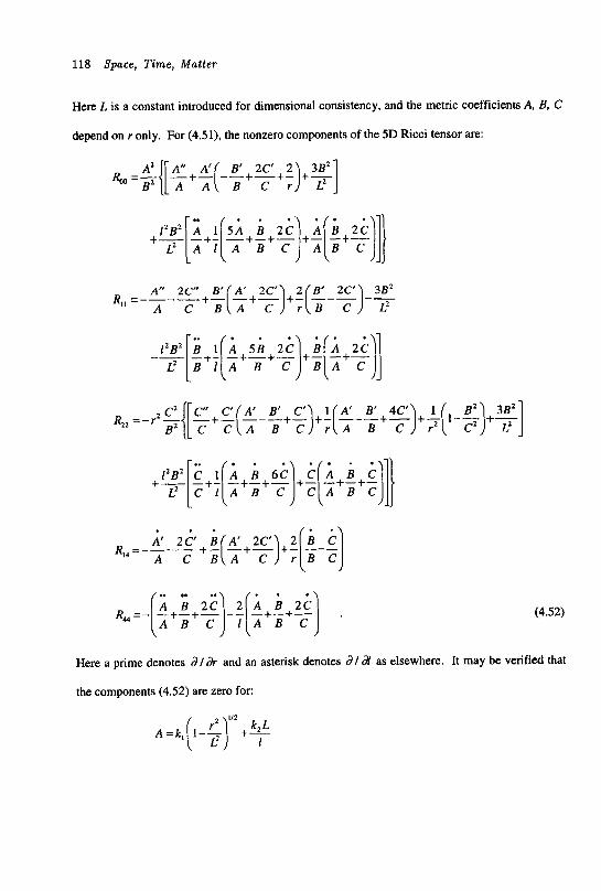
118 Space, Time, Matter
Here L is a constant introduced for dimensional consistency, and the metric coefficients A, B, C
depend on r only. For (4.51), the nonzero components of the 5D Ricci tensor are:
(4.52)
Here a prime denotes a / dr and an asterisk denotes a / d as elsewhere. It may be verified that
the components (4.52) are zero for:

Cosmology and Astrophysics in 5D 119
1 B = (1-r' I L')"'
k, Lz c= 1+- rl
(4.53)
Here &I, k2 and k3 are arbitrary dimensionless constants. The other constant L is a length in the
case where the coordinates r and 1 are lengths, but in principle it can be suppressed using an
appropriate choice of units via L = 1. The same cannot be done for kj, k2 and k3, so (4.53) is a 3-
parameter class.
The properties of matter associated with (4.53) can be evaluated using (4.1). However,
for rnetrics of canonical form there is a more convenient formalism (Mashhoon, Liu and Wesson
1994). In terns of the 4D metric tensor gpv and its associated quantity A,,, = g J 2 , the
induced energy-momentum tensor is
( * Y ( * 7 For metric (4.51). we have $ = A1 A + 2 Cl C and A @ b = A1 A + 2 CI C . It is also
useful to define
rz FSl-- L'
r . . . /. . 3 1' C' 2 A C 2 A 2 C
H3E-i - -+-+- -+- L' Lz[C' AC l [ A C
(4.55)
Then (4.54) becomes
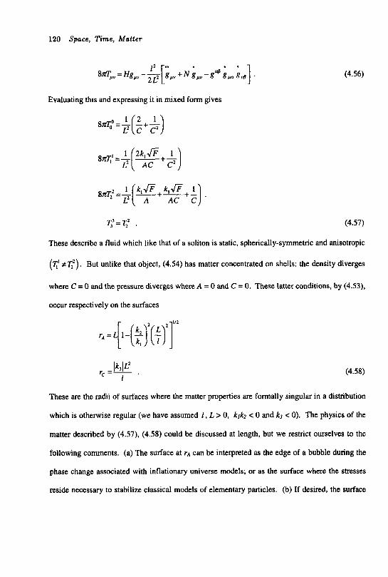
120 Space, Time, Matter
(4.56)
Evaluating this and expressing it in mixed form gives
q=q2 . (4.57)
These describe a fluid which like that of a soliton is static, spherically-symmetric and anisotropic
(T,' # 1;'). But unlike that object, (4.54) has matter concentrated on shells: the density diverges
where C = 0 and the pressure diverges where A = 0 and C = 0. These latter conditions, by (4.53),
occur respectively on the surfaces
(4.58)
These are the radii of surfaces where the matter properties are formally singular in a distribution
which is otherwise regular (we have assumed 1 , L > 0, klk2 < 0 and k3 < 0). The physics of the
matter described by (4.57). (4.58) could be discussed at length, but we restrict ourselves to the
following comments. (a) The surface at rA can be interpreted as the edge of a bubble during the
phase change associated with inflationary universe models; or as the surface where the stresses
reside necessary to stabilize classical models of elementary particles. (b) If desired, the surface
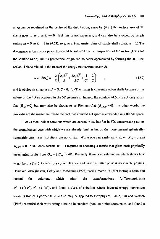
Cosmology and Astrophysics in 5 0 121
at rc can be redefined as the centre of the distribution, since by (4.51) the surface area of 2D
shells goes to zero as C + 0. But this is not necessary, and can also be avoided by simply
setting k3 = 0 so C = 1 in (4.53), to give a 2-parameter class of single-shell solutions. (c) The
divergence in the matter properties could be inferred from an inspection of the metric (4.51) and
the solution (4.53), but its geometrical origin can be better appreciated by forming the 4D Ricci
scalar. This is related to the trace of the energy-momentum tensor via
(4.59)
and i s obviously singular at A = 0, C = 0. (d) The matter is concentrated on shells because of the
nature of the 4D as opposed to the 5D geometry. Indeed, the solution (4.53) is not only Ricci-
flat (RM =0) but may also be shown to be Riemann-flat (RABCD = 0). In other words, the
properties of the matter are due to the fact that a curved 4D space is embedded in a flat 5D space.
Let us then look at solutions which are curved in 4D but flat in 5D, concentrating not on
the cosmological case with which we are already familiar but on the more general spherically-
symmetric case. Such solutions are not trivial. While one can easily write down R,, = 0 and
R,,, = 0 in 5D, considerable skill is required in choosing a metric that gives back physically
meaningful results from G, = 8mb, in 4D. Presently, there is no rule known which shows how
to go from a flat 5D space to a curved 4D one and have the latter possess reasonable physics.
However, Abolghasem, Coley and McManus (1996) used a metric in (3D) isotropic form and
looked for solutions which admit the transformations (diffeomorphisms)
xa -+x"(xs), x4 +x4(x4), and found a class of solutions whose induced energy-momentum
tensor is that of a perfect fluid and so may be applied to astrophysics. Also, Liu and Wesson
(1998) extended their work using a metric in standard (non-isotropic) coordinates, and found a
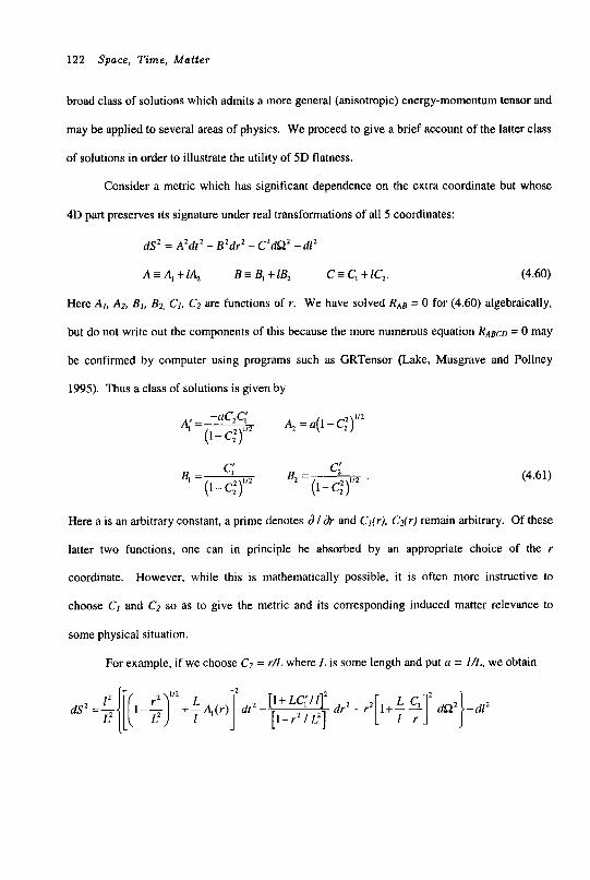
122 Space, Time, Matter
broad class of solutions which admits a more general (anisotropic) energy-momentum tensor and
may be applied to several areas of physics. We proceed to give a brief account of the latter class
of solutions in order to illustrate the utility of 5D flatness.
Consider a metric which has significant dependence on the extra coordinate but whose
4D part preserves its signature under real transformations of all 5 coordinates:
dSz = A2dt2 - B2dr2 - C2dQ2 -dlz
A = A, + 14 B I B, +lB2 C = C, t lC,. (4.60)
Here A,, Az, B1. Bz, C1, CZ are functions of r. We have solved RAE = 0 for (4.60) algebraically,
but do not write out the components of this because the more numerous equation RABCD = 0 may
be confirmed by computer using programs such as GRTensor (Lake, Musgrave and Pollney
1995). Thus a class of solutions is given by
4 = a(1- c,2),/, -ac,c; A'=- I (1- ,),',
(4.61)
Here a is an arbitrary constant, a prime denotes a / & and C/(r), C2(r) remain arbitrary. Of these
latter two functions, one can in principle be absorbed by an appropriate choice of the r
coordinate. However, while this is mathematically possible, it is often more instructive to
choose C , and Cz so as to give the metric and its corresponding induced matter relevance to
some physical situation.
For example, if we choose Cz = r/L where L is some length and put a = I/L, we obtain
dSz = i' { [ [ 1 - $r + f A, ( r ) r dr - [ I + Lc;/l]2 LZ [ 1 - r Z / L']
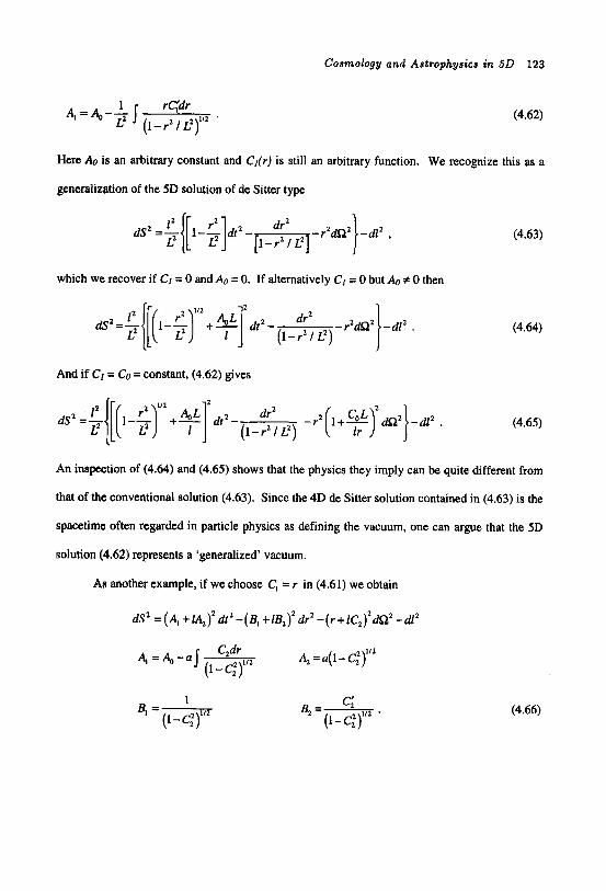
Cosmology and Astrophysics an 5 0 123
A, = 4-- (4.62)
Here & is an arbitrary constant and Cl(r) is still an arbitrary function. We recognize this as a
generalization of the 5D solution of de Sitter type
dS2 =${ [ l-$]dr2 - dr2 - r2d!2’} -d12 , l - r Z / L Z
which we recover if CI = 0 and AO = 0. If alternatively CI = 0 but A0 # 0 then
And if CI = Co = constant, (4.62) gives
(4.63)
(4.64)
(4.65)
An inspection of (4.64) and (4.65) shows that the physics they imply can be quite different from
that of the conventional solution (4.63). Since the 4D de Sitter solution contained in (4.63) is the
spacetime often regarded in particle physics as defining the vacuum, one can argue that the 5D
solution (4.62) represents a ‘generalized’ vacuum.
As another example, if we choose C, = r in (4.61) we obtain
ds2 = (A, + 14)z dt2 -( B, +lB,)’ dr2 - ( r + lC2)zd!22 -d12
A, =&-.I C dr 4=a(l-C:)1’2 (1-ciY
1 4=- (1- ,)“,
c; B, =- ( 1 - C ; Y *
(4.66)
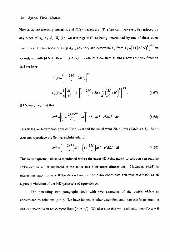
124 Space, T i m e , Matter
Here a, A0 are arbitrary constants and Cz(r) is arbitrary. The last can, however, be replaced by
any other of A], Az, E l , Bz (i.e. we can regard Cz as being determined by one of these other
functions). Let us choose to keep Al(r) arbitrary and determine C2 from C, = [ l + ( a / A ; ) 2 r in
accordance with (4.66). Rewriting Al(r) in terms of a constant M and a new arbitrary function
h(r) we have
A, ( r ) = 1 - - + 2h(r) r 2 : r C,(r)=- :[‘l -+h’ ][ 1--+2h+- 2; ;*(y -+h’ ,’T
If h(r) + 0, we find that
dS2E 1 - - +a1 dr2-dr2 - r2dQ2-d lZ [( 2T I’
(4.67)
(4.68)
This will give Newtonian physics for a + 0 and the usual weak-field limit (2Mh << I ) . But it
does not reproduce the Schwarzschild solution
d S 2 g 1 - - d t 2 - 1+- dr2- r2dQZ-d12 . ( 23 ( 23 (4.69)
This is as expected, since as mentioned before the exact 4D Schwarzschild solution can only be
embedded in a flat manifold if the latter has 6 or more dimensions. However, (4.68) is
interesting since for n # 0 the dependence on the extra coordinate can manifest itself as an
apparent violation of the (4D) principle of equivalence.
The preceding two paragraphs dealt with two examples of the metric (4.60) as
constrained by relations (4.61). We have looked at other examples, and note that in general the
induced matter is an anisotropic fluid (q’ # q2). We also note that while all solutions of &B = 0
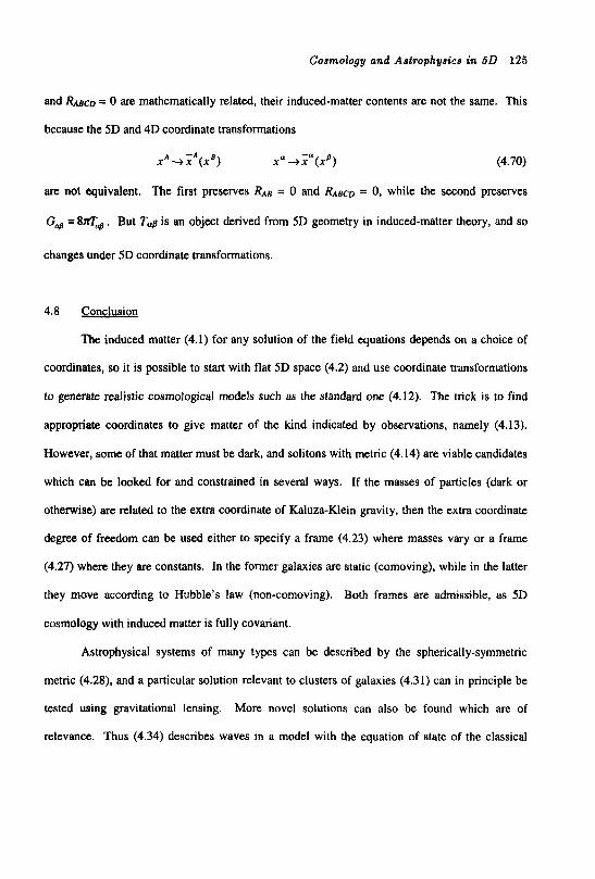
Cosmology and Ast~ophys~cs in 5 0 125
and RABCD = 0 are mathematically related, their induced-matter contents are not the same. This
because the 5D and 4D coordinate transformations
X A + i A ( X B ) x " + i " ( x f l ) (4.70)
are not equivalent. The first preserves RAB = 0 and RABCD = 0, while the second preserves
GN = 8zT4 . But T d is an object derived from 5D geometry in induced-matter theory, and so
changes under 5D coordinate transformations.
4.8 Conclusion
The induced matter (4.1) for any solution of the field equations depends on a choice of
coordinates, so it is possible to start with flat 5D space (4.2) and use coordinate transformations
to generate realistic cosmological models such as the standard one (4.12). The trick is to find
appropriate coordinates to give matter of the kind indicated by observations, namely (4.13).
However, some of that matter must be dark, and solitons with metric (4.14) are viable candidates
which can be looked for and constrained in several ways. If the masses of particles (dark or
otherwise) are related to the extra coordinate of Kaluza-Klein gravity, then the extra coordinate
degree of freedom can be used either to specify a frame (4.23) where masses vary or a frame
(4.27) where they are constants. In the former galaxies are static (comoving), while in the latter
they move according to Hubble's law (non-comoving). Both frames are admissible, as 5D
cosmology with induced matter is fully covariant.
Astrophysical systems of many types can be described by the spherically-symmetric
metric (4.28), and a particular solution relevant to clusters of galaxies (4.31) can in principle be
tested using gravitational lensing. More novel solutions can also be found which are of
relevance. Thus (4.34) describes waves in a model with the equation of state of the classical
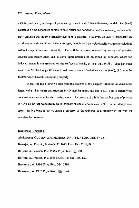
126 Space, Time, Matter
vacuum, and can by a change of parameter go over to a de Sitter inflationary model. And (4.45)
describes a time-dependent soliton, whose matter can be used to describe inhomogeneities in the
early universe that might eventually evolve into galaxies. However, we lack x4-dependent 5D
axially-symmetric solutions of the Ken type, though we have cylindrically-symmetric solutions
without singularities such as (4.50). The cellular structure revealed by surveys of galaxies,
clusters and superclusters can in some approximation be described by solutions where the
induced matter is concentrated on the surfaces of shells, as in (4.51), (4.53). That particular
solution is 5D flat though 4D curved; and broad classes of solutions such as (4.60), (4.61) can be
located which have this intriguing property.
In fact, the main thing we infer from the contents of this chapter is that the universe in the
large, while it has matter and structure in 4D, may be empty and flat in 5D. This is certainly the
conclusion we arrive at for the standard model. A corollary of this is that the big bang of physics
in 4D is an artifact produced by an unfortunate choice of coordinates in 5D. Put in Eddingtonian
terms, the big bang is not so much a property of the universe as a property of the way we
describe the universe.
References (Chamer 4)
Abolghasem, G., Coley, A.A. McManus, D.J. 1996, J. Math. Phys. 37, 361.
Banerjee, A., Das, A., Panigrahi, D. 1995, Phys. Rev. D 2, 6816.
Billyard, A,, Wesson, P.S. 1996a, Phys. Rev. D S , 731.
Billyard, A., Wesson, P.S. 1996b, Gen. Rel. Grav. 28, 129.
Bruckman, W. 1986, Phys. Rev. D34,2990.
Bruckman, W. 1987, Phys. Rev. D36,3674.
Cosmology and Astrophysics in 5 0 127
Chatterjee, S., Wesson, P.S., Billyard, A. 1997, Nuovo Cim., Bl& 1667.
Chinea, F.J., Femandez-Jambrina, L., Senovilla, J.M.M. 1992, Phys. Rev. D45,481.
Clement, G. 1986, Gen. Rel. Grav. 18, 137.
Frolov, V.P., Zelnikov, A.I., Bleyer, U. 1987, Ann. Phys. (Leipzig) 44,371.
Gott, J.R., Rees, M.J. 1987, Mon. Not, Roy. Astron. SOC. 227,453.
Gross, D.J., Perry, M.J. 1983, Nucl. Phys. B B , 29.
Henriksen, R.N., Wesson, P.S. 1978, Astrophys. Space Sci 53,429.
Home, J.H., Horowitz,G.T. 1992, Phys. Rev. D46, 1340.
Kolb, E. 1989, Astrophys. J. 344, 543.
Lake, K., Musgrave, P.J., Pollney, D. 1995, GRTensor Version 1.19 (Dept. of Physics, Queen’s
University, Canada).
Liu, H., Wesson, P.S., Ponce de Leon, J. 1993, J. Math. Phys. 3,4070.
Liu, H., Wesson, P.S. 1998, Gen. Rel. Grav., 3 , 5 0 9 .
Mashhoon, B., Liu, H., Wesson, P.S. 1994, Phys. Lett. B 331,305.
Matos, T. 1994, J. Math. Phys. 2, 1302.
Myers, R.C., Perry, M.J. 1986, Ann. Phys. (New York) 172,304.
Ponce de Leon, J. 1988, Gen. Rel. Grav. 20,539.
Ponce de Leon, J. 1993, Gen. Rel. Grav. 25, 1123.
Ponce de Leon, J., Wesson, P.S. 1993, J. Math. Phys. 34,4080.
Rindler, W. 1977, Essential Relativity (2nd ed., Springer, Berlin), 185.
Robertson, H.P., Noonan, T.W. 1968, Relativity and Cosmology (Saunders, Philadelphia), 367,
413.
Roque, W.L., Seiler, W.M. 1991, Gen. Rel. Grav. 23, 1151.
128 Space, Time, Matter
Ruiz, E., Senovilla, J.M.M. 1992, Phys. Rev. D G , 1995.
Senovilla, J.M.M. 1990, Phys. Rev. Lett. 64,2219.
Tikekar, R., Patel, L.K., Dadhich, N. 1994, Gen. Rel. Grav. 26,647.
Wesson, P.S. 1978, Cosmology and Geophysics (Oxford U. Press-Hilger, New York).
Wesson, P.S. 1991, Astrophys. J. 378,466.
Wesson, P.S. 1992, Phys. Essays (Toronto) 5,561.
Wesson, P.S., Liu, H., Lim, P. 1993, Phys. Lett. B =,69.
Wesson, P.S. 1994a, Astrophys. J. 436, 547.
Wesson, P.S. 1994b, Astrophys. J. 420, L49.
Wesson, P.S., Liu, H. 1995, Astrophys. J. 440, 1.
Wesson, P.S., Liu, H. 1998, Phys. Lett. B 432,266.
Will, C.M. 1991, Gravitation: A Banff Summer Institute (eds. Mann, R., Wesson, P.S., World
Scientific, Singapore), 439.
5. SD ELECTROMAGNETISM
"I felt a new kind of spark" (Madonna, Buenos Aires, 1995)
5.1 Introduction
Kaluza, we recall, realized that when there is no matter present the equations of 5D
general relativity contain those of 4D Einstein gravity and 4D Maxwell electromagnetism
(Kaluza 1921). Klein extended this approach to quantum theory (Klein 1926), and ever since
Kaluza-Kltin theory has been regarded as a unified theory of gravity and electromagnetism.
More recently, though, various workers have shown that induced-matter theory as outlined in
Chapter 2 explains the phenomenlogical properties of matter if the traditional geometry of
Kaluza-Klein theory is broadened to include dependency on the extra coordinate. However, it is
true that in this approach photons still occupy a special place. In the present chapter, we wish to
see how electromagnetism fits into a general 5D geometry.
Thus we start with a 5D metric that depends on x4 = 1 and redo the algebra that puts it
into a form where we recognize the electromagnetic potentials (Section 5.2). Then we work out
the fully covariant form of the 5D geodesic equation (Section 5.3). We will find that the latter
now contains x4-dependent terms which are in principle important for testing 5D field theory.
These terms are small in practice, however, so subsequently we drop x4-dependence and present
a class of exact solutions in 5D which extends the soliton class by including electric charge
(Section 5.4). This class includes the case where the 4D part of the metric describes a
Schwanschild-like black hole, and to elucidate the effects of charge in 5D we then give an
analysis of the electrodynamics involved in this case, finding that it leads to unexpected
differences from 4D (Section 5.5). Finally, we return to the field equations and the question of
129
130 Space, Time, Matter
induced matter, and present the former in a way that allows us to evaluate the energy density of
the electromagnetic field (Section 5.6). We will find that while 5 D electromagnetism has been
much studied, it yet contains some surprises.
5.2 Metrics and Potentials
The reduction of a 5D metric to a 4D one where the potentials can be recognized as those
of gravity and electromagnetism has been done by various workers under the assumption of x4-
independence. In this and the following section, we follow Wesson and Ponce de Leon (1995)
and look at the fully-covariant situation.
The 5 D interval is given by
dSz = ~ ~ ~ d x ~ d x ' . (5.1)
If we wish to investigate the 4D interval ds included in this, it is convenient to define a unit 5D
vector Y A , tangent to the fifth dimension:
(5.2)
This will enable us to split the 5 D metric into a part parallel to Y A and a 4D part orthogonal to
it. Thus we define a projector:
g A B Y A8 -E 'yAyS 7 (5.3)
where by (5.2)
This has
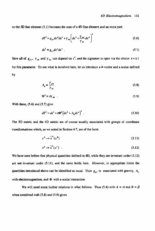
5D Electromagnetism 131
so the 5D line element (5.1) becomes the sum of a 4D line element and an extra part:
\l
dsl =g,,dr'dxy . (5.7)
Here all of g,,, yu and can depend on x4, and the signature is open via the choice &=*I
for this parameter. To see what is involved here, let us introduce a 4-vector and a scalar defined
by
A =!& (5.8)
Q1=qu . (5.9)
Y44
With these, (5.6) and (5.7) give
dS1 = a!r2 +&'(dx4 + A,dr"r . (5.10)
The 5D metric and the 4D metric are of course usually associated with groups of coordinate
transformations which, as we noted in Section 4.7. are of the form
X A + X"(X") (5.1 1)
x ~ + ~ p ( x v ) . (5.12)
We have seen before that physical quantities defined in 4D, while they are invariant under (5.12)
are not invariant under (5.11), and the same holds here. However, in appropriate limits the
quantities introduced above can be identified as usual. Thus g,, is associated with gravity, A,,
with electromagnetism, and with a scalar interaction.
We will need some further relations in what follows. Thus (5.4) with A = 01 and B =
when combined with (5.8) and (5.9) gives
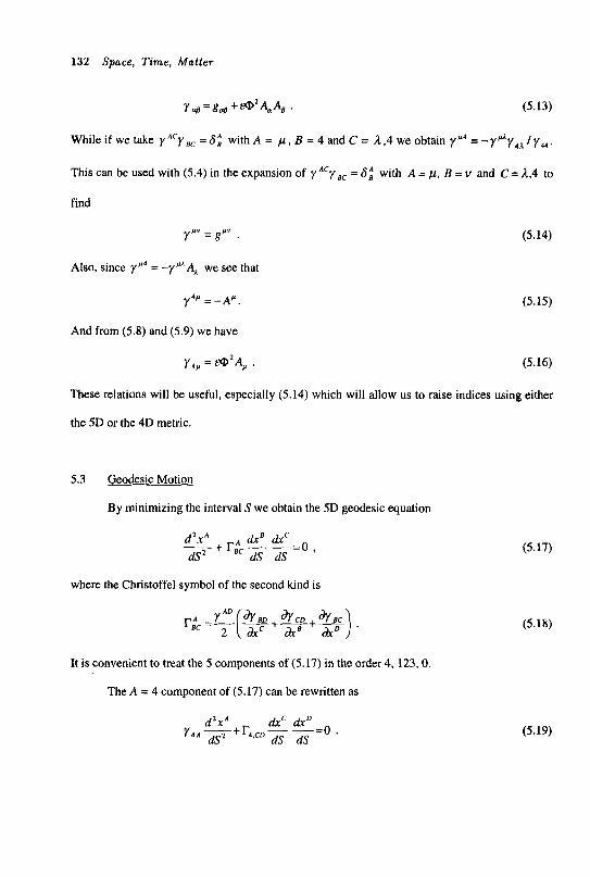
132 Space, Time, Matter
y@=g, +&@AeAp . (5.13)
Whileifwetake y A C y e c = S i withA = p L B = 4 a n d C = L,4weobtain yp4=-yMy41.1y44.
This can be used with (5.4) in the expansion of yACyec = 6; with A = p, B = v and C = 1,4 to
find
y’I” = g ’ V . (5.14)
Also, since y P 4 = -y@A, we see that
y4M = -A’. (5.15)
And from (5.8) and (5.9) we have
y4p =&‘A,, . (5.16)
These relations will be useful, especially (5.14) which will allow us to raise indices using either
the 5D or the 4D metric.
5.3 Geodesic Motion
By minimizing the interval S we obtain the 5D geodesic equation
drn drc - + r&- -=o , d Z x A dS2 dS dS
where the Christoffel symbol of the second kind is
It is convenient to treat the 5 components of (5.17) in the order 4, 123.0.
The A = 4 component of (5.17) can be rewritten as
(5.17)
(5.18)
(5.19)
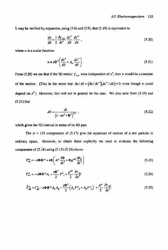
5D Electromagnetism 133
It may be verified by expansion, using (5.8) and (5.9), that (5.19) is equivalent to
where n is a scalar function:
(5.20)
(5.21)
From (5.20) we see that if the 5D metric ycD were independent of x4, then n would be a constant
of the motion. [This in the sense that dnldS = (&/ dx”)(dx” I d s ) = 0 even though n could
depend on $.I However, this will not in general be the case. We also note from (5.10) and
(5.21) that
ds ds= (l-m~1@2)”* ’
(5.22)
which gives the 5D interval in terms of its 4D part.
The A = 123 components of (5.17) give the equations of motion of a test particle in
However, to obtain these explicitly we need to evaluate the following ordinary space.
components of (5.18) using (5.13)-(5.16) above:
(5.24)
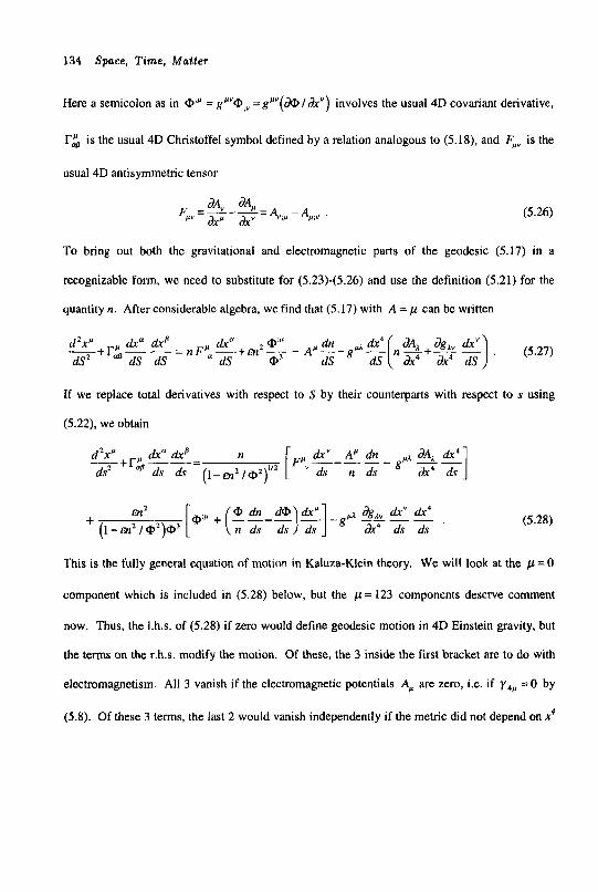
134 Space, Time, Matter
Here a semicolon as in @’” = g”v@;v = g P ” ( ~ / & ” ) involves the usual 4D covariant derivative,
r$ is the usual 4D Christoffel symbol defined by a relation analogous to (5.18), and F,, is the
usual 4D antisymmetric tensor
To bring out both the gravitational and electromagnetic parts of the geodesic (5.17) in a
recognizable form, we need to substitute for (5.23)-(5.26) and use the definition (5.21) for the
quantity n. After considerable algebra, we find that (5.17) with A = p can be written
d 2 x p dx” dxa dx“ z@’” dn dw4 ( JA, agly d x v ) -+I-# - - = n F p -+m - - Ap--g4- n-+- - . dS‘ @ dS dS a dS @’ dS dS ax4 ax4 dS
(5.27)
If we replace total derivatives with respect to S by their counterparts with respect to s using
(5.22), we obtain
(5.28)
This is the fully general equation of motion in Kaluza-Klein theory. We will look at the p = 0
component which is included in (5.28) below, but the p = 123 components deserve comment
now. Thus, the 1.h.s. of (5.28) if zero would define geodesic motion in 4D Einstein gravity, but
the terms on the r.h.s. modify the motion. Of these, the 3 inside the first bracket are to do with
electromagnetism. All 3 vanish if the electromagnetic potentials A,, are zero, i.e. if y4,, = 0 by
(5.8). Of these 3 terms, the last 2 would vanish independently if the metric did not depend on x4
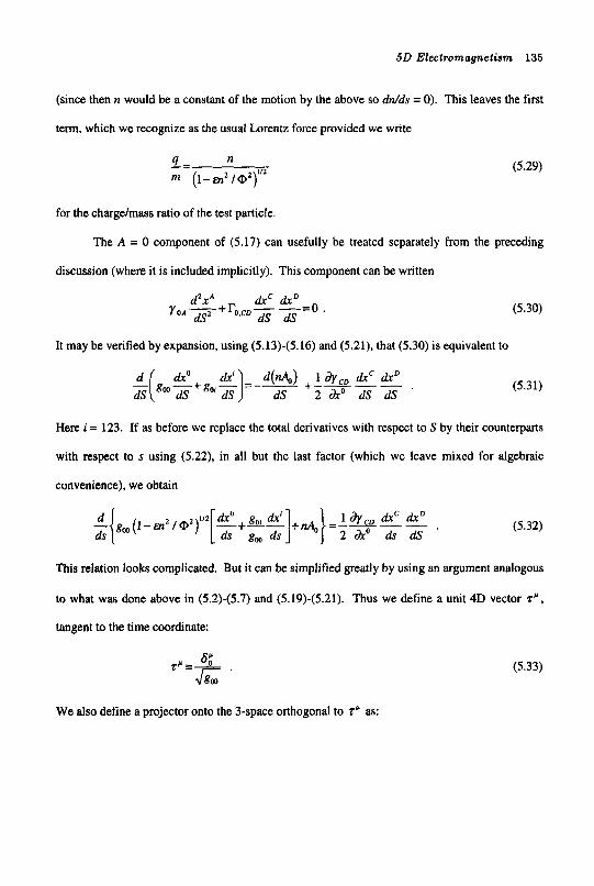
5 0 Electromagnetism 135
(since then n would be a constant of the motion by the above so ddds = 0). This leaves the first
term, which we recognize as the usual Lorentz force provided we write
(5.29) 4- n -_ m (1 - Enz I 0 2 ) 1 ' 2
for the chargelmass ratio of the test particle.
The A = 0 component of (5.17) can usefully be treated separately from the preceding
discussion (where it is included implicitly). This component can be written
-0 d'x A dxc dxD Y OA x+ r0,crl x-
It may be verified by expansion, using (5.13)-(5.16) and (5.21). that (5.30) is equivalent to
d ( dro dS dS dS 2 axo dS dS
dr'] d(&) +-A"- l a / drc dxD - g , - - + g , ' ~ =--
(5.30)
(5.31)
Here i = 123. If as before we replace the total derivatives with respect to S by their counterparts
with respect to s using (5.22), in all but the last factor (which we leave mixed for algebraic
convenience), we obtain
(5.32)
This relation looks complicated. But it can be simplified greatly by using an argument analogous
to what was done above in (5.2)-(5.7) and (5.19)-(5.21). Thus we define a unit 4D vector z' ,
tangent to the time coordinate:
(5.33)
We also define a projector onto the 3-space orthogonal to z' as:

136 Space, Time, Matter
(5.34)
Then Am = doj = 0 analogous to (5.5). and the 4D line element (5.7) becomes the sum of a time
part and a space part:
This can be rewritten and factored to give
(5.35)
(5.36)
provided the square of the spatial 3-velocity is defined by vz =Aovivi and the velocity itself is
defined by
(5.37)
This is an element of ordinary space divided by an element of proper time in (5.35), and so is the
appropriate definition of a 3-velocity analogous to the usual one for a 4-velocity. We can now
use (5.36) to substitute for the term in square brackets in (5.32). The result is
de l~?)',dr~dr~ ds 2 ax' ds dS '
- ---
where e is a scalar function:
(5.38)
(5.39)
The relations (5.38) and (5.39) are equivalent to the geodesic (5.30). From (5.38) we see that if
the 5D metric yco were independent of xo, then e would be a constant of the motion. However,
this will not in general be the case. We do note, though, that (5.39) bears a strong resemblance
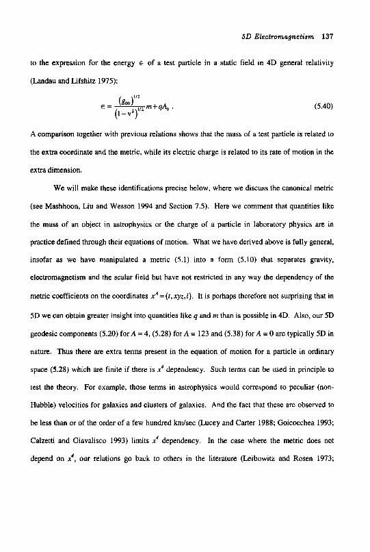
5 0 Electromagnetism 137
to the expression for the energy E of a test particle in a static field in 4D general relativity
(Landau and Lifshitz 1975):
(5.40)
A comparison together with previous relations shows that the mass of a test particle is related to
the extra coordinate and the metric, while its electric charge is related to its rate of motion in the
extra dimension.
We will make these identifications precise below, where we discuss the canonical metric
(see Mashhoon, Liu and Wesson 1994 and Section 7.5). Here we comment that quantities like
the mass of an object in astrophysics or the charge of a particle in laboratory physics are in
practice defined through their equations of motion. What we have derived above is fully general,
insofar as we have manipulated a metric (5.1) into a form (5.10) that separates gravity,
electromagnetism and the scalar field but have not restricted in any way the dependency of the
metric coefficients on the coordinates x A =(r,xyz,l) . It is perhaps therefore not surprising that in
5D we can obtain greater insight into quantities like q and rn than is possible in 4D. Also, our 5D
geodesic components (5.20) for A = 4, (5.28) for A = 123 and (5.38) for A = 0 are typically 5D in
nature. Thus there are extra terms present in the equation of motion for a particle in ordinary
space (5.28) which are finite if there is x4 dependency. Such terms can be used in principle to
test the theory. For example, those terms in astrophysics would correspond to peculiar (non-
Hubble) velocities for galaxies and clusters of galaxies. And the fact that these are observed to
be less than or of the order of a few hundred k d s e c (Lucey and Carter 1988; Goicoechea 1993;
Calzetti and Giavalisco 1993) limits x4 dependency. In the case where the metric does not
depend on x4, our relations go back to others in the literature (Leibowitz and Rosen 1973;
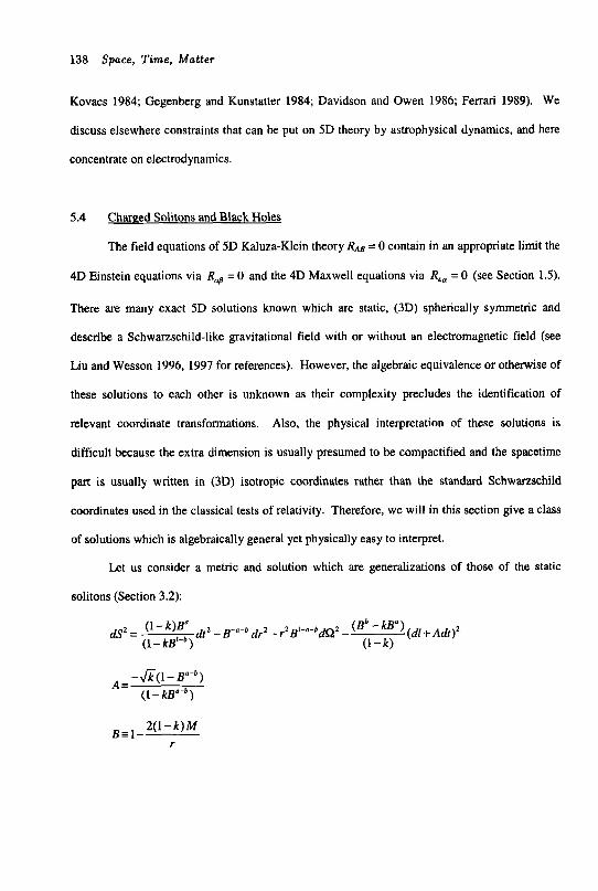
138 Space, Time, Matter
Kovacs 1984; Gegenberg and Kunstatter 1984; Davidson and Owen 1986; Ferrari 1989). We
discuss elsewhere constraints that can be put on 5D theory by astrophysical dynamics, and here
concentrate on electrodynamics.
5.4 Charzed Solitons and Black Holes
The field equations of 5D Kaluza-Klein theory RAB = 0 contain in an appropriate limit the
4D Einstein equations via RM = 0 and the 4D Maxwell equations via R4, = 0 (see Section 1.5).
There are many exact 5D solutions known which are static, (3D) spherically symmetric and
describe a Schwarzschild-like gravitational field with or without an electromagnetic field (see
Liu and Wesson 1996, 1997 for references). However, the algebraic equivalence or otherwise of
these solutions to each other is unknown as their complexity precludes the identification of
relevant coordinate transformations. Also, the physical interpretation of these solutions is
difficult because the extra dimension is usually presumed to be compactified and the spacetime
part is usually written in (3D) isotropic coordinates rather than the standard Schwarzschild
coordinates used in the classical tests of relativity. Therefore, we will in this section give a class
of solutions which is algebraically general yet physically easy to interpret.
Let us consider a metric and solution which are generalizations of those of the static
solitons (Section 3.2):
-&(I- Ba-b) (1- kBa-b)
A=
2(1-k)M B i l - r
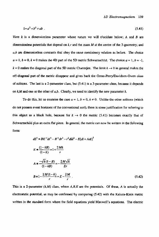
5 0 Electromagnetism 139
l=a’+b*+ub . (5.41)
Here k is a dimensionless parameter whose nature we will elucidate below; A and B are
dimensionless potentials that depend on k,r and the mass M at the centre of the 3-geometry; and
a,b are dimensionless constants that obey the same consistency relation as before. The choice
u = 1, b = 0, k = 0 makes the 4D part of the 5D metric Schwarzschild. The choice a = 1, b = -1,
k = 0 makes the diagonal part of the 5D metric Chattejee. The limit k + 0 in general makes the
off-diagonal part of the metric disappear and gives back the Gross-PerryfDavidson-Owen class
of solitons. The last is a 2-parameter class, but (5.41) is a 3-parameter class, because it depends
on k,M and one or the other of u,b. Clearly, we need to identify the new parameter k.
To do this, let us examine the case a = 1, 6 = 0, k # 0. Unlike the other solitons (which
do not possess event horizons of the conventional sort), there is some justification for refemng to
this object as a black hole, because for k + 0 the metric (5.41) becomes exactly that of
Schwarzschild plus an extra flat piece. In general, the metric can now be written in the following
form:
dSz = BE-ldt’ - K’dr’ - r Z d n Z - E(dl+ Ad?)’
-&( l -B) 2 M & A = =-- ( 1 - k B ) Er
(5.42) r r
This is a 2-parameter (k,M) class, where A,B,E are the potentials. Of these, A is actually the
electrostatic potential, as may be confirmed by comparing (5.42) with the Kaluza-Klein metric
written in the standard form where the field equations yield Maxwell’s equations. The electric
2 M ( l - k ) - 2M B s l - - E - - .
140 Space, Time, Matter
field has only a radial component ( E , , not to be confused with E above). In terms of the usual
Faraday tensor F, I dAo / A a -dA, /Ao of (5.26), i t is given by
The associated invariant is
8M2k E'r4
I = F @ F - -2E(F,0 )2=- - OB-
(5.43)
(5.44)
By(5 .42) for r + m , w e h a v e B + I , E - 1 and A + - 2 M & I r . Thelastshouldbe - Q / r
to agree with Coulomb's law at large distances from the source charge Q. This allows us to
identify the parameter k with conventional units restored as
k = - Q Z 4GM2 '
(5.45)
Using this in (5.42)-(5.44) allows us to sum up the quantities of interest (valid for any r ) as
follows:
Q' E=l t - 2 Mr
(5.46)
Already here we can see that a quantity Q2/Mr that depends on the combination of Q and M
comes into the 5D solution, whereas only the quantities M/r and @/? that depend seDaratelv on
Q and M come into the corresponding 4D (Reissner-Nordstrom) solution.
The preceding paragraph concerns the case a = 1, 6 = 0, k # 0. However, the choice
a = 1, 6 = 0 is smoothly contained in the range - 2 / J ? - < ( a , b ) < 2 / f i allowed by the
5 0 Electromagnetism 141
consistency relation given by the last member of (5.41). Thus we identify the whole 3-parameter
class of exact solutions (5.41) as charged solitons.
5.5 CharEd Black Hole Dvnamics
In this section, we will combine what we learned about geodesic motion in Section 5.3
with the solution presented in Section 5.4 to study the dynamics of a test particle with charge 4
and mass m in orbit around a 5D black hole with charge Q and mass M.
The metric for the latter is (5.42). which is independent of x4 so n of (5.21) is a constant
of the motion. That relation is then the first integral of the last component of the geodesic
equation. The spacetime components are given by (5.28). The equations of motion are thus
(5.47)
By (5.29) or (5.48) directly, we obtain the asymptotic (r + -, E + 1) value for the charge/mass
ratio of the test particle as
4 n -=- rn ( I+ nZ)”’
4 n = ( m 2 - q‘)“’ (5.49)
The second term on the r.h.s. of (5.48) is an extra force not present in 4D electrodynamics, but it
is tiny for classical as opposed to quantum situations because it depends on (q/mJ2, which with
conventional units restored is q2 / Gm’ << 1. For any r, we can rewrite (5.48) and (5.49) as
142 Space, Time, Matter
(5.50)
where E = ( l + Q 2 1 2 M r ) as before. We can evaluate this for index a = 1 in what might be
112 called the standard approximation, specified by 1q l 4 << 1, M / r << 1,
For this approximation, rk I M l r z , Fo' z Q / r2 and we obtain
uIz3 <<uo I (g") .
(5.51)
which is of course true in many situations.
There are two cases of (5.47)-(5.49) which can be studied without approximation and are
illustrative: (i) Q = 0,4 # 0 and (ii) Q f 0, q = 0. For (i) we have by (5.45) k = 0 and we have by
(5.42) E = 1 , A = 0 and B = 1-2Mh. The metric (5.42) is
(5.52)
which is just a neutral 4D Schwarzschild black hole plus an extra flat dimension. The motion of
a charged particle around such a black hole from (5.47)-(5.49) is given by
(5.53)
(5.54)
In other words, for this case the constant of the motion associated with the extra dimension is
essentially the charge-mass ratio of the test particle, and the 4D motion is geodesic in the
Einstein sense. For (ii), we have by (5.49) n = 0, so by (5.46)-(5.48) there comes
5 0 Electromagnetism 143
d2xa d.2 dxy - dr2 + r;--=o. ds ds
(5.55)
(5.56)
The 4D motion is again geodesic in the Einstein sense, while (5.55) implies that the metric (5.42)
loses its extra part and becomes effectively 4D. Using (5.46), in the large-r approximation we
find B s (1- 2M / r + Q2 / 2Mr) and BE-’ P (1- 2 M / r+ Q’ / r’), so the metric is
-r2 dQ2 . ds2 E (1 - ?+ 5) dt’ - dr2 (1 - 2M I r+ Q’ / 2Mr)
This can be compared to the Reissner-Nordstrom solution of Einstein’s theory:
-r2dQ’. dr2 ds’= I--+- dt2- ( 2r :”) ( l - 2 M / r + Q Z / r 2 )
(5.57)
(5.58)
We see that they agree in goo but not in gli. That is, at large distances the 3-space associated
with the ‘5D’ black hole (5.57) is different from that associated with the 4D black hole (5.58).
The difference will in practice be minor, since the mass equivalent of the energy associated with
the central charge will be small in most situations (GQ’ /c4r‘ <<I). However, this discrepancy
prompts us to ask about the consistency of the electromagnetic field associated with the solutions
(5.42). To be precise: The solutions (5.58) satisfy the 4D field equations G4 =87rT4 in terms of
the Einstein tensor and a standard energy-momentum tensor describing an electrostatic field,
whereas (5.57) or (5.42) satisfy 5D field equations RAB = 0 with nothing on the right-hand side;
so what is the effective energy-momentum tensor of the 5D solutions (5.42) if they are viewed in
4D7
The answer to this can be given here by anticipating results from the following section on
the induced matter associated with non-diagonal metrics such as (5.10). For the charged black-
144 Space, Time, Matter
hole solutions (5.42) we find that the energy density associated with the electromagnetic field is
given by
(5.59)
This has its conventional form, implying that the 5D solutions (5.42) do not show departures
from the 4D ones in the far field even though they may in the near field.
The above concerns the electromagnetic field. Returning to dynamics, we expect small
differences in the orbits of particles about the central mass, because the Lagrangian associated
with the 5D charged black hole (5.42) differs from that associated with the 4D charged black
hole (5 .58) and also from that associated with the 5D neutral soliton (3.6). The latter was
investigated extensively in Chapter 3 with regard to the classical tests of relativity in the solar
system. And while we do not expect there to be significant electromagnetic effects in that
situation, it is instructive to see how charges alter 5D dynamics. To examine this, let us rewrite
(5.42) as
~ = ~ ~ - l i ~ - ~ - ~ i * - r ~ ( e z +s in20$2) -E( i+~ i )Z . (5.60)
Here r = dr / dd etc., where h is an affine parameter, and we can assume that the orbit is confined
to the plane O=n I 2 with b = 0. Then from (5.60) we obtain in the usual way 3 constants of the
motion:
j = B E - ~ ~ - E ( ~ + A ~ ) A
(5.61)
Rearranging these gives the 5-velocities in the case where A = S (so L = I ) as
5 0 Electromagnetism 145
i = EB-' ( j -mi)
6, = hr-'
i = - n E - ' - E A B - ' ( j - n A ) . (5.62)
For Q = 0 ( E = l , A = 0) these give r = B-'j, 6)=hr-' and l = - n , which are identical to the results
of Chapter 3 for the case where the metric parameters are Q = 1, b = 0. If & the test charge is
q = 0, the 5D Lagrangian (5.60) becomes identical to the 4D one, so there is no difference in the
dynamics. This applies obviously to photons, which perforce have q = 0; so the classical tests
involving redshift, light bending and radar ranging are of minor interest. There remains,
however, the question of what happens with massive particles which could conceivably have
q # 0 and the analog of the perihelion test. To investigate this, we can take the Lagrangian (5.60)
[with A = S], substitute into it for the constants of motion (5.61) [with Q, A f 0 for now] and
rearrange to get:
Changing to a variable u = l/r as before, this yields
(5.63)
(5.64)
This formula could provide the basis for a detailed investigation of the orbit of a charged test
particle about a charged source, but for now we look at the simpler case Q = 0 (q # 0), when
(5 .64) gives
(5.65)
Taking d I d4 of this and assuming the orbit is not perfectly circular (du / d4 # O), we obtain
146 Space, Time, Matter
(5.66)
This is a special case of equation (3.34) found before (it corresponds to d = 1 + nz, e = 0 for the
constants in the previous case). The test particle has a precession per orbit which in our notation
is
(5.67)
Here, the first term is the one quoted in the usual approach using Einstein's theory, while the
second is an extra one that is necessarily positive. It exists because the Lagrangian (5.60) or
metric (5.42) looks like the usual 4D one but augmented by a boost in the extra dimension
[i = dl 1 dS= - n = - q(mZ - qZ)-"' by (5.62) and (5.49)]. The extra term in (5.67) could in
principle be significant for a test particle with an appropriate charge/mass ratio.
The last relation (5.67) and others we have derived in this section have concentrated on
the classical effects of charge, insofar as we have taken a class of 5D charged black-hole
solutions (5.42) with a classical test particle. The latter has q/G"2rn<<l with conventional
units restored. However, i t would be feeble not to comment on the case q / G"2rn>>l, which is
typical of elementary particles and usually treated by quantum theory. That there is a problem in
treating particles with large chargelmass ratios or fluids with large charge densities was
appreciated by Kaluza (192 I). The quantization of charge was attributed to compactification by
Klein (1926), but this only partly addresses the problem with dynamics and runs into other
difficulties (see Chapter 1). However, an interesting suggestion that may resolve the problem
posed by particles with y I G'%>> I was made by Davidson and Owen (1986). It is simply that
such particles move on spacelike as opposed to the usual timelike geodesics of a 5D space. An
5 0 Electromagnetism 147
inspection of our equations shows that it is possible to reformulate the dynamics in this case so
that whiled,? c 0 we still have d? > 0, so 4D causality is maintained. This idea is intriguing but
requires further study.
5.6 Field Euuations and Induced Matter
The induced 4D energy-momentum tensor T, for metrics which satisfy the 5 D field
equations RAB = 0 is usually evaluated algebraically (by rewriting the latter equations as
G, =8nTas) or by computer (by using programs that sort terms which are 4D and 5 D in
nature). However, both approaches have been developed primarily for metrics with g,, = O
which describe matter with no electromagnetic potentials. Therefore, we will in this section
cany out an analysis with these included that is analogous to that for neutral matter in Section
2.5. We aim particularly at evaluating the electromagnetic part of T, for the charged 5 D black
holes discussed in Sections 5.4 and 5.5 above.
The line element dSZ=g,dXAdrB for electromagnetic problems is usually taken as
(5.10), which it is convenient to rewrite in matrix form:
(5.68)
Here A" = g4Ag etc. as usual, and we use the same notation as before with hats added to the 4D
parts of 5 D quantities if there is a danger of confusion with the pure 4D quantities. For situations
with electromagnetic fields, it is natural for reasons given above to consider the case where
g, = g,(x") . Then the nonzero 5D Christoffel symbols of the second kind are:
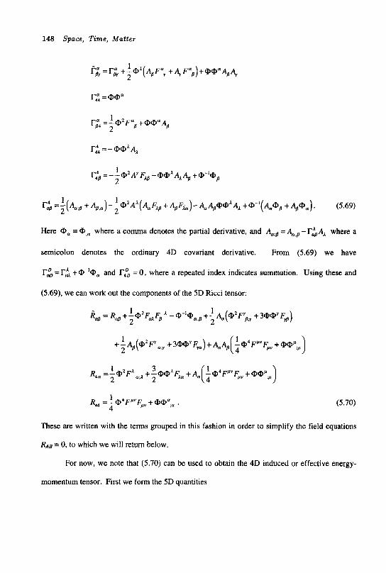
148 Space, Time, Matter
Here @, = a,, where a comma denotes the partial derivative, and &;, where a
semicolon denotes the ordinary 4D covariant derivative. From (5.69) we have
rz = l-: + @-loa and I'4", = 0 , where a repeated index indicates summation. Using these and
(5.69), we can work out the components of the 5D Ricci tensor:
1 1 2 2
R4 = R4 + -@'FdFa - + - &(@ZF\;r + 3QW FM)
These are written with the terms grouped in this fashion in order to simplify the field equations
RAB = 0, to which we will return below.
For now, we note that (5.70) can be used to obtain the 4D induced or effective energy-
momentum tensor. First we form the 5D quantities
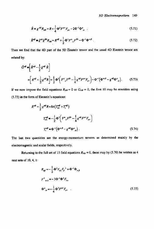
5D Electromagnetism 149
(5.72)
Then we find that the 4D part of the 5D Einstein tensor and the usual 4D Einstein tensor are
related by:
-W1(cPu~p -g@@pir). (5.73)
If we now impose the field equations RAE = 0 or GAB = 0, the first 10 may be rewritten using
(5.73) in the form of Einstein's equations:
1 2
Rd --g@R=&('&? +q@)
The last two quantities are the energy-momentum tensors as determined mainly by the
electromagnetic and scalar fields, respectively.
Returning to the full set of 15 field equations RAE = 0, these may by (5.70) be written as 4
neat sets of 10,4, 1:
1 R = - - Q Z F F @ 2 d P
(5.75)
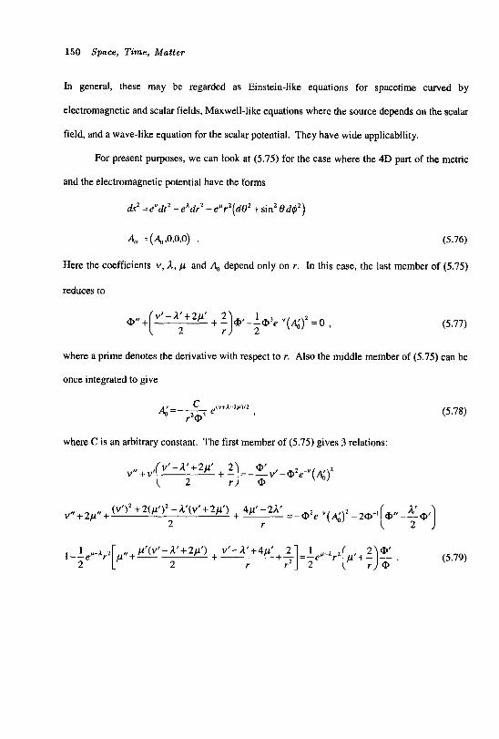
150 Space, Time, Matter
In general, these may be regarded as Einstein-like equations for spacetime curved by
electromagnetic and scalar fields, Maxwell-like equations where the source depends on the scalar
field, and a wave-like equation for the scalar potential. They have wide applicability.
For present purposes, we can look at (5.75) for the case where the 4D part of the metric
and the electromagnetic potential have the forms
ds’ =evdtz -e’dr’ -e”r’(d@ +sin28dgZ)
Here the coefficients v , d, p and A,, depend only on r. In this case, the last member of (5.75)
reduces to
*,,+( v’-d;+2P’ (5.77)
where a prime denotes the derivative with respect to r. Also the middle member of (5.75) can be
once integrated to give
(5.78) 4- c e ( v + l - 2 C 1 / 2
r 2 a 3
where C is an arbitrary constant. The first member of (5.75) gives 3 relations:
(v‘-di+2p’ v” + v‘
(VY + 2 t ~ ~ -xw+w) + 4 p t - 2 ~ ’ =-a2e-v(4 , ’ )2 -2Q-, r
v” + 2p1* + 2
(5.79)

5D Electromagnetism 151
The 5 equations (5.77)-(5.79) constitute a complete set for the 5 unknowns CP, A,,, V , A and ~1 .
It may be verified by hand that the charged soliton solutions (5.41) satisfy (5.77)-(5.79), or by
computer that they satisfy the equivalent set RAE = 0.
The charged black-hole solutions (5.42) are an algebraically simple subset of (5.41), and
for reasons given in Section 5.5 we are particularly interested in evaluating the energy density of
the electrostatic field in this case. Putting (5.42) into (5.74) and using (5.43). (5.44) gives
2 1 g"(F,,) -zgw F'" F,, 2
- BM2k E'r4
-- (5.80)
By (5.45) k = Q Z / 4 M 2 and by (5.46) for r + m we have E + 1, B + 1, SO T$+Q214r4 .
This result, quoted as (5.59) in Section 5.5, is of conventional form and shows that the induced-
matter approach is valid for electromagnetic fields.
5.7 Conclusion
The 5D metric with gravitational, electromagnetic and scalar potentials is commonly
taken as (5.10) to distinguish these fields. The geodesic equation gives a new scalar associated
with motion in the extra dimension (5.21), which comparison with the motion in spacetime
(5.28) reveals to be connected with the chargelmass ratio of a test particle (5.29). However, the
new scalar is not a constant of the motion unless the metric is independent of x4, and the
charge/mass ratio is in general a function of all 5 coordinates. The time component of the 5D
geodesic defines a scalar (5.39) analogous to the particle energy (5.40) in general relativity. The
152 Space, Time, Matter
static, neutral solitons which we met before as the standard 1-body solutions in 5D can be
generalized to a 3-parameter class with charge (5.41). In the case where the embedded 4-space
in the neutral limit is Schwarzschild, we can speak in the general case of a 2-parameter class of
charged 5D black holes (5.42). The motion of a test particle in orbit around such an object
shows interesting effects, but even when the 5D metric becomes effectively 4D (5.57) it does not
exactly reproduce the Riessner-Nordstrom metric (5.58) of general relativity. The field
equations for x4-independent electromagnetic problems are (5.75) and have wide applicability;
but the energy density of the electrostatic field for the charged 5D black holes as calculated by
the induced matter approach (5.80) is somewhat conventional.
Notwithstanding this, there are some odd results connected with 5D electromagnetism.
The fact that these are small in the classical domain suggests that future work in this area should
focus on the particle domain.
References (Chauter 5 )
Calzetti, D., Giavalisco, M. 1993, Astrophys. J . 406,388.
Davidson, A., Owen, D.A. 1986, Phys. Lett. B U , 77.
Ferrari, J.A. 1989, Gen. Rel. Grav. 21,683.
Gegenberg, J., Kunstatter, G. 1984, Phys. Lett. A@, 410.
Goicoechea, L.J. 1993, Astron. Astrophys. 269, L9.
Kaluza, T. 1921, Sitz. Preuss. Akad. Wiss. 33,966.
Klein, 0. 1926, 2. Phys. 37, 895.
Kovacs, D. 1984, Gen. Rel. Grav. 16,645.
Landau, L.D., Lifshitz, E.M. 1975, The Classical Theory of Fields (Pergamon, Oxford), 251.
5 0 Electromagnetism 153
Leibowitz, E., Rosen, N. 1973, Gen. Rel. Grav. 4,449.
Liu, H.. Wesson, P.S. 1996, Phys. Lett. Bm, 420.
Liu, H., Wesson, P.S. 1997, Class. Quant. Grav. l4, 1651.
Lucey, D., Carter, D. 1988, Mon. Not. Roy. Astron. Soc. 235, 1177.
Mashhoon, B., Liu, H., Wesson, P.S. 1994, Phys. Lett. B&l, 305.
Wesson, P.S., Ponce de Leon, J. 1995, Astron. Astrophys. 294, 1.
6. THE CANONICAL METRIC AND THE mPTH FORCE
"To be believable it has to be measurable" (Francis Everitt, Stanford, 1996)
6.1 Introduction
In Chapter 2 we analysed several solutions of the 5D field equations RAB = 0, some of
which depended on the extra coordinate x4 = I , and ended by giving a general prescription for x4-
dependent metrics that allows us to evaluate their effective or induced 4D matter. In Chapter 6
we started with an x4-dependent form of the metric suited to 5D electromagnetism, but then
concentrated on the x4-independent case in order to obtain results on 4D electrodynamics. Both
of these approaches made use of the algebraic freedom inherent in unrestricted 5D Riemannian
geometry to choose the 5 coordinates 2 freely, with resultant simplifications for the metric
tensor gAB and other objects such as the Ricci tensor RAB that figure in the theory. In general
relativity, this is commonly called a choice of coordinates, but in particle physics the analogous
procedure is called a choice of gauge. In the present chapter, we will start with a general
discussion of gauges, but then concentrate on a new choice which is especially suited to
dynamics. The main result is that there is an extra or fifth force inherent in 5D theory which has
no counterpart in 4D general relativity.
6.2 Gauges in Kaluza-Klein Theory
The choice of a gauge in physics, like the choice of a map projection in geography,
depends on what one wants to achieve. And the vast majority of gauges, if chosen arbitrarily, are
therefore of little practical use. However, the original electromagnetic gauge of Kaluza-Klein
theory, which consists in gM = g&'), g,- = %(x ' ) , g, =-1, is useful, because while it
154
The Canonical Metric and the Fifth Force 155
imposes the x‘hdependent or “cylinder” condition it allows one to identify the potentials of
Maxwell’s theory. Likewise the “matter” gauge wherein g, = g4(xA) , g,= = 0,
g, = g,(xA) is useful, because it allows one to go from RAB = 0 to C , = 8 f l , and identify the
4D Einstein tensor and the induced energy-momentum tensor with its associated properties of
matter.
A natural question, and one we wish to answer before proceeding, concerns the status of
the 5D analog of the 4D harmonic gauge. The latter is extensively used in general relativity,
notably to describe gravitational waves in the weak-field limit of Einstein’s theory (see e.g.
Weinberg 1972). The corresponding 5D harmonic gauge, in terms of the Christoffel symbol and
the determinant of the metric, is given by
These are 5 conditions, but since rtB is not a tensor the conditions (6.1) are not 5D covariant.
This is the classical analog of the situation in quantum field theory involving non-covariant
gauges (Leibbrandt 1994). In physical terms, fields which are split on one hypersurface of the
metric will in general be mixed on another hypersurface, implying a problem when comparing
5D and 4D physics. By analogy with the latter, we assume that the metric is close to flat:
g A B = q A B + h A B I f l A B = * l , IhABl<<l . (6.2)
The gauge conditions (6.1) with (6.2) now read
(6.3)
We note in passing that these conditions are very restrictive, being first-order relations that must
be applied to second-order field equations. The latter in the approximation (6.2) become
156 Space, Time, Matter
This 5D box operator can be written in terms of its 4D counterpart and extra terms, so the field
equations (6.4) read
That is, free waves in 5D become waves with sources in 4D. Regarding the r.h.s. of (6.5) as a
4D source, solutions can be written at least in principle using Green's functions (Myers and
Perry 1986; it may be necessary to carry out an imaginary coordinate transformation or Wick
rotation depending on the sign of the last part of the metric). But while the 5D harmonic gauge
shares the general property of modem Kaluza-Klein theory, namely that source-free equations in
5D become ones with sources in 4D, it is clear that it has problems with application to physics.
It is possible, if physics is not the prime concern, to decompose the 15 5D field equations
RAB = 0 into sets of 10, 4, 1 4D field equations without the imposition of a specific gauge. This
involves using an extended version of the lapse and shift technique commonly employed in
general relativity (Misner, Thome and Wheeler 1973; Hawking and Ellis 1973; Wald 1984). A
preliminary application of this confirms what may be inferred from previous work, namely that
the 10 Einstein-like equations describe physics on a 4D hypersurface, while the 4 Maxwell-like
or conservation equations and the 1 wave-like equation for the scalar field depend on how that
surface is embedded in 5D (Sajko, Wesson and Liu 1998; see also Section 2.5). However, it is
still true that application to a particular problem in physics requires the choice of a specific gauge
or form of the metric.
A form which we have met before in several contexts can succinctly be restated here as:
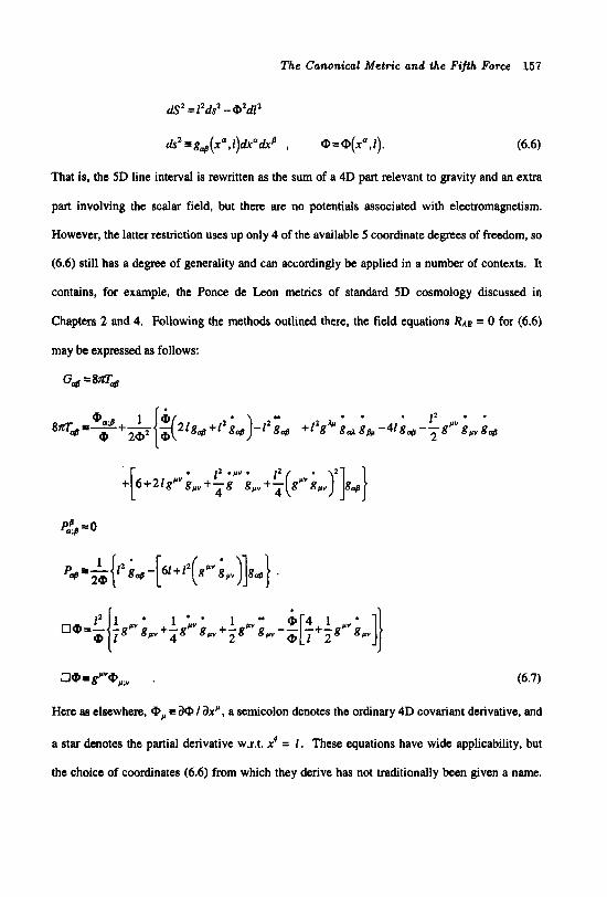
T h e Canonical Metric and ihe Fifth Force 157
dS1 =lzdsz -6'dl'
That is, the 5D line interval is rewritten as the sum of a 4D part relevant to gravity and an extra
part involving the scalar field, but there are no potentials associated with electromagnetism.
However, the latter restriction uses up only 4 of the available 5 coordinate degrees of freedom, so
(6.6) still has a degree of generality and can accordingly be applied in a number of contexts. It
contains, for example, the Ponce de Leon metrics of standard 5D cosmology discussed in
Chapters 2 and 4. Following the methods outlined there, the field equations RAE = 0 for (6.6)
may be expressed as follows:
q$=8m;,
c)Q=g'v9,;" . (6.7)
Here 88 elsewhere, 9, = a 6 I ax', a semicolon denotes the ordinary 4D covariant derivative, and
a star denotes the partial derivative w.r.t. x4 = I . These equations have wide applicability, but
the choice of coordinates (6.6) from which they derive has not traditionally been given a name.
158 Space, Time, Matter
In view of more recent developments, it is appropriate to refer to (6.6) as the "semi-canonical"
gauge.
The true canonical gauge is anived at by using the remaining degree of coordinate
freedom to set Q Z ( x A ) in (6.6) to unity (Mashhoon, Liu and Wesson 1994). Introducing a
constant length L to preserve physical dimensions, we then have
This metric leads to significant simplification of the induced-matter relations and also of the
geodesic equations (5.28). The price one pays for this is that the 4D sector now harbors effects
of the fifth dimension, which in general show up as departures from the usual laws of motion.
However, such effects are Machian in the sense that they can be viewed as the influence of the
rest of the universe on the properties of a local particle (Jordan 1955; Bekenstein 1977; Wesson
1978; Shapiro 1993). Such cosmological effects can be couched in terms of the time-variability
of particle rest mass or the gravitational "constant", the choice being largely irrelevant because
the two parameters occur in conjunction in gravitational problems. Limits on time-variability of
the latter may be used to constrain the former, so we know that dynamical effects of the
canonical gauge are at most of order 10.'' yr-' (Will 1992). However, if the world is 5D in
nature and depends significantly on the extra dimension, these effects are necessarily f m , and
can be expressed in terms of a fifth force which is quite different from other known forces
(Mashhoon, Wesson and Liu 1998). In view of the fundamental importance of this issue, we
proceed to examine the main aspects of it in the following sections.
The Canonical Metric and the Fifth Force 159
6.3 Th e Field Eauations and the Cosmolonical Constant
Let us apply the canonical gauge (6.8) to the field equations (6.7). Then the middle
member remains virtually unchanged, the last member becomes a constraint, and the first set
reads
. .
. p * . 6+21 gcv g,, +--g’” g,,
4 (6.9)
When g, = 0 , as in general relativity, these equations read just GM =3gM I L’. These are
Einstein’s equations with a cosmological constant A = 3 / L’, which is small if L is a large
cosmological length. We see that from the viewpoint of Kaluza-Klein theory, the cosmological
constant of Einstein’s theory is a kind of artifact produced by a certain reduction from 5D to 4D.
The preceding paragraph identified the cosmological constant from the field equations in
a procedure which appears to be straightforward (Mashhoon, Wesson and Liu 1997). However,
we recall that in general relativity this parameter can be regarded as defining a density and
pressure for the vacuum via p = A I8n = - p with the characteristic equation of state p + p = 0
(see Section 1.3). These properties of matter can be regarded as part of the energy-momentum
tensor Td , and it is really the equation of state which defines the vacuum. In modem Kaluza-
Klein theory, the field equations are RAB = 0. These are scale-free, and it would run counter to
the philosophy of the theory to introduce a constant like A with the physical dimensions of L-’
or T -2. But in the induced-matter picture, the effective energy-momentum tensor will in general
contain terms which we identify as ordinary matter and other terms which we by default regard
as relating to the vacuum. The question then arises of whether it is possible to interpret exact 5D
160 Space, Time, Matter
solutions whose equation of state is p t p = 0 in terms of something like the cosmological
constant.
To examine this, let us consider 2 exact solutions which have appeared in the literature
and which we will return to later in a different form (Mashhoon, Liu and Wesson 1994; Liu and
Mashhoon 1995; Sections 7.2, 7.3). We give them here in a scale-free or self-similar form
(Henriksen, Emslie and Wesson 1983):
l 2 dSz = -[dT2 3 - ezT'Jj(dRz t RzdQ')]-dlz .
(6.10)
(6.1 1)
Both metrics are canonical, and in both the coordinates T, R are dimensionless, with the physical
dimension of dS carried by the coordinate I . For (6.10). the Kretschmann scalar is
K F RABCD ItABcD = 432a2 I l'R6. This and all components of the Riemann-Christoffel tensor are
zero if the dimensionless constant a is zero. For (6.11), all components of the Riemann-
Christoffel tensor are zero anyway. Thus both (6.10) and (6.1 1) can describe 4D curved spaces
embedded in flat 5D spaces (see Section 4.7). When we look at the induced energy-momentum
tensor, we find that for both solutions 8 f l , = g, where g, refers to the 4D part of the 5-
metric. This we recognize as the signature of a vacuum; but an ambiguity exists as to whether
we should raise an index using the 4-metric or the 5-metric. The former procedure does not make
much physical sense, while the latter procedure gives 8np = 8 f l : = 3/ 1' , 81p, = -8M,' = -3/1*
(Wesson 1997). Thus the equation of state is p + p = 0, but both properties of matter depend on
the extra coordinate, leading to fundamental questions about the nature of the cosmological
constant.
The Canonical Metric and the Fifth Force 161
This parameter is, of course, at the centre of a muddle in 4D physics. The cosmological-
constant problem basically consists in a contradiction between the small value of this parameter
as derived from general relativity and cosmological data, and the large value inferred from
quantum field theory and its zero-point fields (see Weinberg 1989 and Ng 1992 for reviews).
Based on what was stated above, a resolution of this problem is available at least in principle in
5D physics. It is simply that the induced energy-momentum tensor follows from a solution of
local field equations, so the density and pressure of the vacuum depend on the situation and do
not necessarily define a universal constant.
6.4 The huations of Motion and the Fifth Force
In this section we will derive the equations of motion using a Lagrangian approach for
the canonical metric (6.8). This involves a choice of coordinates about which we wish to make a
few preliminary comments. The coordinates in (6.8) can be constructed by taking a 4D
hypersurface in the 5D manifold, and regarding the lines normal to this hypersurface as the extra
coordinate. These lines will be geodesics, and proper length along them will be the extra
coordinate x4 = 1 . This method of constructing a coordinate system is the 5D analog of how the
synchronous coordinate system of general relativity is set up in 4D. It is based on the
assumption that one can construct a 4D hypersurface in 5D with no obstruction. This coordinate
system breaks down only if the coordinate lines in the fifth dimension cross. Therefore, apart
from pathological situations, our coordinates are always admissible within a finite interval along
the fifth dimension.
The equations of motion are obtained by minimizing the distance between two points in
=O. If h is an arbitrary affine parameter along the path, this relation can be
162 Space, Time, Matter
written S Ldd = 0 , where using (6.8) the quantity which is commonly referred to as the [I I Lagrangian is
(6.12)
The path in 5D is described by xa = xa(d) , 1 = I @ ) . The momenta and the equations of motion
are then given as usual by
dL pa = &dxa I dd)
dPa - -_- dd axa
dL P'=d(dIldil) (6.13)
(6.14)
Defining ua = aka Ida , U' P dl l d d and 8 8 L2 = (1' I L2)g4uauB - (u') ' . we then have for the
momenta
Pa =(3$ The corresponding equations of motion are
U' Pf =-F
We interject at this point the observation that the (conserved) super-Hamiltonian is
(6.15)
(6.16)
(6.17)
(6.18)
as expected. Now we resume our working, and choose d = s so gaauau8 = 1, to manipulate the
equations of motion into the form
The Canonical Metric and the Fifth Force 163
(6.19)
(6.20)
Here r'& is the usual 4D Christoffel symbol of the second kind. With the parameter along the
path as 4D proper time, 8 = (1' / L')-(dl Ids)', and the last equation can be written as
1 2 a1
Substituting for 8 in (6.19) and using (6.21), the 4D equations of motion can be written
du' -+rLuauy = F" ds
The extra component of the equation of motion (6.21) can be rewritten as
(6.21)
(6.22)
(6.23)
This completes the formal part of our analysis. Basically, if the coordinates and metric are put
into the canonical form (6.8), the 4D equations of motion (6.22) show that ordinary geodesic
motion is modified by the addition of a quantity P' which is a kind of force per unit inertial
mass. (This is the analog in the canonical gauge of the extra terms we found in the
electromagnetic gauge in Section 5.3.) The new force is nonzero if the 4D metric depends on the
fifth coordinate (dg* / a1 f 0) and there is motion in the fifth dimension (dl / ds # 0 ) . The rate
of motion in the fifth dimension is given by a solution of (6.23) and is in general nonzero.
164 Space, Time, Matter
As a technical aside, we note that the latter equation can be once integrated. In (6.23), if
we write z = l / l , Z = u “ u a ( d g , / d f ) andputL= 1,thatequationbecomes
Multiplying both sides of this by -22’ (ddds) gives
which can be integrated to yield
(6.24)
Here C is an arbitrary constant and a = z(so) is evaluated at some fiducial value of the 4D
interval. For the special case 2 = 0 when the 4D pan of the metric does not depend on the extra
coordinate, (6.24) is solved by z = a cosh (s - SO) with C = -d . In general, (6.24) gives on
replacing the original variable the relation
($) =12-iexp[~~Zdl] i4 c (6.25)
This gives the square of the velocity in the extra dimension in terms of the 4D interval and a
fiducial value of the extra coordinate (dl Ids = 0 at 1 = l o ) , and is a useful relation.
Returning now to the 4D equations of motion (6.22), we note that the new force F” (per
unit inertial mass) is necessarily connected to the existence of the fifth dimension. For from
(6.22) we can form the scalar quantity
(6.26)
The Canonical Metric and the Fifth Force 165
which has no 4D analog and brings out the dependencies noted above. Another way to see what
is involved here is to start from the 4D scalar uauo = 1 , where we recall that in our approach this
means ua(s)g4(x”,l)ua(s)= 1. The application of the total (4D covariant) derivative D/ds to
this, dong with the observation that Dg4 Ids = (&@ /dl ) (dl lds) , results in
F a g ~ u a + u a u a - - + u a g 4 F B dl = O . d l ds
(6.27)
This rearranged gives back (6.26). We see that the existence of the force (per unit inertial mass)
F’ , and its associated scalar F*up (which is a kind of power). follows from the fact that we
have used the 4D interval s to characterize the motion in a 5D manifold. This makes sense from
a practical point of view, because we have a body of 4D physics which we wish to interpret in
terms of 5D geometry. However, it is important to realize that Fpup # 0 is a unique indication
of the existence of at least one higher dimension.
To appreciate this, consider for the moment 4D Einstein gravity with other known forces.
For example, the Lorentz force of electrodynamics obeys the relation Du’/ds=(q/m)F’,u’
where q h is the chargelmass ratio of a test particle and Fpv is the (Faraday) field tensor. The
antisymmetry of the latter means that Fp,upuv = 0 , so F, = (q Im)Fpvuv obeys F,u’ = 0 . As
another example, the force due to the pressure of a perfect fluid can be seen to obey a similar
relation by considering the energy-momentum tensor 7””’ = (p+ p)u”u” - pg” . This obeys
P”:” = 0 or
( P + P ) , ” U ” U “ +(P+p)u’,,”p+p)u’uv”-p,,g’’ = o . (6.28)
166 Space, Time, Matter
This can be multiplied by up , and the term (p + p)u” ;v uVuH dropped, because by taking the
covariant derivative of u’u,, = 1 , we have upiv up = 0 (see above). Then there results
(P+P)U’: , = - p p ” (6.29)
which put back into (6.28) gives
(6.30)
Again by virtue of upup = 1 , this implies FPup = 0. This result and the preceding one an not so
much meant as a reminder of known physics, as illustrations of the fact that timelike motions in
4D general relativity with other known forces obey equations of motion of the form
Du” Ids = F p with F,u’ = 0.
Conversely, the new force (6.22) derived in this section has F,u’ # 0 . Thus at least part
of the new force (per unit inertial mass) F” of (6.22) must be non4D in origin. To see this
explicitly, we can express F’ as the sum of a component (N’) normal to the 4-velocity up of
the particle and a component (P’) parallel to it. Thus F’ = N’ t P’ , where
(6.31)
(6.32)
Clearly the normal component could be due to ordinary 4D forces (it obeys N’u, = O by
construction), but there exists no 4D analoe of the uarallel comDonent (it is P” = u”F“u, and
The Canonical Metric and the Fifth Force 167
has P’u, t O in general). This anomalous “fifth” force is therefore a consequence of the
existence of the extra dimension.
6.5 Comments on the Fifth Force
In the preceding section, we saw that the components of the fifth force normal and
This is simply a parallel to the 4-velocity are both proportional to (agM /dZ)(dZ/ds)ua.
consequence of employing the canonical coordinate system, and the fact that in this system
dynamics is concentrated in the dependence of the spacetime metric on the fifth coordinate.
However, it is useful to show that the form of the resulting equation for the fifth force (6.32) is
general. We proceed to do this, and then make some comments on the fifth force in specific
cases.
Let us consider a general 5D line element in the standard form for electromagnetism:
dS’=d~’-Q~(dl+A, ,dx’ )~ . (6.33)
Here ds2 = gMdxadxa i s the spacetime metric as before, while CP and A,, are scalar and vector
potentials. If gM, @ and A,, are independent of the fifth coordinate I as in the traditional
Kaluza-Klein theory, then using the results given in Chapter 5 it is straightforward to show that
the fotce P (per unit inertial mass) on a particle is orthogonal to its 4-velocity ua and there is
no fifth force.
imagine now a &&t change of coordinates in 5D such that the new spacetime metric has
the form
ds‘ = g,(x’,l)dx%a . (6.34)
168 Space, Time, Matter
The 5D geodesic remains invariant under the coordinate transformation. However, in 4D the
force on the particle picks up an anomalous component to the 4-velocity, while the
normal component is expected to differ only slightly from F". To compute the new parallel
component (fifth force), we simply differentiate
g * ( X ' , I ) U a U @ = 1 (6.35)
with respect to proper time s. Hence
y a p dl du' d l ds ds
g*,$u u u +- -u~u@+2gw- l4*=O,
where the first term on the 1.h.s. can be written as
(g$,r +g4 ,8 - ~ g y , , ) u y ~ o ~ ~ = 2 g , r ; ~ ~ ~ * ~ @ .
(6.36)
(6.37)
using symmetries under the exchange of c1 and p. It follows that equation (6.36) can be
expressed as
or using the definition of force per unit inertial mass
Thus in the new perturbed coordinates a timelike fifth force appears which is given by
(6.38)
(6.39)
(6.40)
This is the same expression as (6.32). However, the nature of the argument presented here
implies that the fifth force has this form generally, regardless of the coordinate system employed.
Let us suppose that careful observations did indeed reveal a fifth force of the type
described above. That is, suppose the net force on a particle were found to consist of an ordinary
The Canonical Metric and the Fifth Force 169
component due to the four fundamental interactions, plus an anomalous timelike component
proportional to the particle’s four-velocity as in (6.40). Furthermore, let us suppose we insisted
on interpreting these observations in terms of 4D physics (i.e., excluding a possible fifth
dimension). Then the net force on the particle could be expressed as
D -(mua) = m ( N a + P a ) ds
Using uau” = 1 and uaDua Ids = 0 we then obtain
p a = B U ” ,
(6.41)
(6.42)
where. /3 a m-’ dmlds . That is, the particle’s mass would change with its proper time if we
maintained that the world had only 4 dimensions when in fact it had 5. (This would presumably
be a slow process, given the observational constraints alluded to in Sections 6.2 and 4.2.)
Another related possibility, which we will come back to later, is to identify particle mass as the
fifth coordinate. Then the extra component of the equation of motion (6.23) would give the rate
of change of mass directly. In either case, we see that if there is a fifth dimension then it could
show up as a variation in mass.
6.6 A TOY Model
The force F’ of (6.22) and its associated scalar power (6.26) will exist for a wide class
of solutions of the field equations RAB = 0. What we wish to do here is to take the simplest
model available and examine its consequences.
We start from the canonical metric (6.8) and put L = 1, g @ ( x ” , l ) = i-’q4. Then
170 Space, Tame, Matter
dS2 = q48dxadra -d12 (6.43)
and is flat. It might be useful to recall here that metrics which are 5D flat can correspond in
certain systems of coordinates to metrics which are 4D curved, so we should not assume that
(6.43) is devoid of physics. However, in the coordinates of (6.43). the geodesic equation
obviously leads to dxA I dS = constants in terms of the 5D interval. However, in terms of the 4D
interval, given by ds2 = g,dxadxa = l ~ 2 q ~ d x a d x a , we have qosuaua = 1’ and the last
component of the equations of motion (6.23) reads
(6.44)
Writing this as d[l-’dl lds]/ds = 0 we get
I = c , ~ & , (6.45)
where C5 is an arbitrary constant and f l = l-’dl I ds is a constant independent of the (4D) motion.
[In more complicated situations, one may start with equation (6.25).] The first four components
of the equations of motion (6.22) read
1 dl dr” dx” 1 ds ds ds
= P - - , =- - - (6.46)
where was just defined. If we express F” in terms of its components normal and parallel to
the 4-velocity u” (see above), then N” = 0 and P” = pU”. On performing a translation in 4D
to produce an appropriate definition of the origin, and denoting 4 other arbitrary constants by
C, , we have from (6.46) that
The Canonical Metric and the Fifth Force 171
x" = c,, eB . (6.47)
So by (6.45) and (6.47), the motion in 5D in terms of the interval in 4D is summed up simply by
x" = CAe&.
This solution depends on 5 arbitrary constants (CA). But only 4 are independent, as the
metric (6.43) with U " E dx" /dS implies the consistency relation U AUA = 1. To see what is
involved here, let us consider the relationships between quantities in 5D, 4D and 3D when the
4D metric is qM = (tl, - 1, - 1, - 1). We can define 3D velocities v' = dx' / dt ( i = 123) as
usual, where by (6.47) we have
The 4D interval ds' = l-2q&adxa then invites us to write
(6.48)
(6.49)
Modulo the sign choice involved in taking the square root, we therefore have C, = C,,/3(1- v')"~,
That is, C, = Cop in the frame when v = ( vivi)"' is zero. The 5D and 4D intervals (again
modulo a choice of sign) are related via
(6.50)
172 Space, T i m e , Mat t e r
where we have used (6.45). The velocities in terms of the 5D interval and the velocities in terms
of the 4D interval are related, since dr” la3 = (dx” lds)(dsldS). Using (6.45), (6.47) and (6.50)
we have
(6.51)
This shows, as we stated above, that the 5-velocities obey dr” Ids = constants. Also, the
consistency relation we stated at the beginning of this paragraph, namely U”U, = 1, now reads
C,’ = B’(C,’ - C: - C l - C:) . This gives C, = KO in the frame where v is zero, agreeing with
what was noted above. The upshot of these considerations is that there is consistency between
how we describe the motion in 3D, 4D and 5D; and that in the toy model we are looking at the
motion in the extra dimension is such that B = l-’dl Ids is a constant.
In general, therefore, the 4D equation of motion (6.46) involves a force F’ and a power
F’u, that are both nonzero:
F’ = pup
F”u, = p . (6.52)
The value of the constant fl is not determined by the toy model being used here, and neither is its
sign. These things require the use of more sophisticated models.
6.7 Conclusion
Gauges in 5D field theory control to a certain extent what physical insights ensue, and in
this chapter we have concentrated on the canonical one (6.8) which brings out effects of the extra
coordinate. For this gauge, the 5D field equations show that while the cosmological constant

The Canonical Metric and the Fifth Force 173
may be identified by comparison with the 4D equations of general relativity, this parameter does
not fit naturally into the induced-matter picture, being replaced by the more general concept of
properties for the vacuum which are determined locally. The canonical gauge has major
implications for dynamics. It defines the Lagrangian (6.12) which leads to equations of motion
in 4D spacetime (6.22) and the extra dimension (6.23). The former involve a modification to the
usual 4D motion of a test particle which has the nature of a new force (per unit inertial mass).
This is nonzero if the metric depends on the extra coordinate (which in general it will if there is
induced matter present) and if there is movement in the extra dimension (which in general there
will be since we have no reason to presume things are static there and no gauge freedom left to
impose this). The total force P’ of (6.22) has a velocity-contracted scalar associated with it,
namely F’u, of (6.26), which is a kind of power and is nonzero under the noted conditions.
This is an indicator of the existence of at least one extra dimension, since known (4D)
interactions involve F’u, = 0. The total force F” can be expressed in terms of the component
normal to the 4-velocity N’ and the component parallel to it P’ , as in (6.31) and (6.32). The
former obeys N’u’ = 0, so strictly speaking it is the fact that P’u’ # 0 which would indicate the
existence of (at least) a fifth dimension. It is actually a general property of x‘-dependent metrics
in 5D theory that there appears a new timelike or fifth force P’ (6.40). If, however, one tried to
interpret this from a 4D perspective, it could manifest itself as a time variation in particle mass as
in (6.42). A similar relation (6.52) results when one calculates the rate of change of the extra
coordinate in a toy model. Both variations are of course constrained by data on dynamics, and in
particular by limits on the time variation of the gravitational interaction, to which we have
alluded earlier in this chapter and in previous ones.
174 Space, Time, Matter
Given this, two questions occur. First, why has the fifth force escaped detection by
traditional dynamical tests such as those applied in the solar system? Second, what new ways
are available to look for it?
References (Chapter 6)
Bekenstein, J.D. 1977, Phys. Rev. D l5, 1458.
Hawking, S.W., Ellis, G.F.R. 1973, The Large-Scale Structure of Space-Time (Cambridge U.
Press, Cambridge), 44.
Henriksen, R.N., Emslie, A.G., Wesson, P.S. 1983, Phys. Rev. D 27, 1219.
Jordan, P. 1955, Schwerkraft und Weltall (Vieweg, Braunschweig).
Leibbrandt, G. 1994, Non-Covariant Gauges (World Scientific, Singapore).
Liu, H., Mashhoon, B. 1995, Ann. Phys. (Leipzig) 4,565.
Mashhoon, B., Liu, H., Wesson, P.S. 1994, Phys. Lett. B 331,305.
Mashhoon, B., Wesson, P.S., Liu. H. 1998, Gen. Rel. Grav., 3 0 , 5 5 5 .
Misner, C., Thome, K., Wheeler, J.A. 1973, Gravitation (Freeman, San Francisco), 506.
Myers, R.C., Perry, M.J. 1986, Ann. Phys. (New York) 172,304.
Ng, Y.J. 1992, Int. J. Mod. Phys. DL, 145.
Sajko, W.N., Wesson, P.S., Liu, H. 1998, J. Math. Phys. 2,2193.
Shapiro, 1.1. 1993 Quantum Gravity and Beyond - Essays in Honour of Louis Witten (eds.,
Mansouri, F., Scanio, J.J., World Scientific, Singapore), 180.
Wald. R. 1984, General Relativity (U. of Chicago Press, Chicago), 255.
Weinberg, S. 1972, Gravitation and Cosmology (Wiley. New York), 162,253.
Weinberg, S. 1989, Rev. Mod. Phys. 6_, 1.
The Canonical Metric and the Fifth Force 175
Wesson, P.S. 1978, Cosmology and Geophysics (Oxford U. Press-Hilger, New York).
Wesson, P.S. 1997, Int. J. Mod. Phys. D 6,643.
Will, C.M. 1992, Int. J. Mod. Phys. D 1, 13.
7. CANONICAL SOLUTIONS AND PHYSICAL QUANTITIES
“General relativity will eventually overtake the rest of physics”
(George Ellis, Waterloo, 1997)
7.1 Introduction
In Chapter 6 we found that when the 5D metric is written in the canonical form, where
the extra dimension is explicit, the equations of motion yield in a relatively straightforward way
a fifth force which is unlike those of classical electromagnetism or 4D general relativity.
However, this force does not manifest itself in the solar system at the level of order 0.1% set by
the classical tests. It also does not appear to manifest itself in cosmological systems, though the
level here is less stringent due to observational uncertainties. In the present chapter we will find
that there is a simple yet fundamental reason for this: canonical solutions exist in which the fifth
force is zero. That is, there are exact solutions of the 5D field equations which possess a simple
symmetry and result in the same dynamics as 4D general relativity.
This means that we have to look elsewhere for the effects of the fifth dimension. The
best option for detection would appear to be a gyroscope experiment in Earth orbit. We
discussed this before in Chapter 3 for the soliton metric, but we revisit the problem here for the
1-body metric in canonical form and give a detailed analysis. We will find that while the orbit of
the gyroscope is the same as in general relativity, the precession of its spin axis is different.
We will then return to, and make concrete, an issue which has been considerably
discussed in the literature and which we have mentioned at several places in this account, namely
the connection between the extra coordinate x4 and the rest mass of a test particle m. This is a
manifestation of Mach’s principle (Chapter 1); and for the induced-matter interpretation of 5D
176
Canonical Solutions and Physical Quantities 177
relativity, we know that when the metric is written in a certain form, dependency on x4 generally
implies matter consisting of particles with finite rest masses, while independency implies matter
consisting of photons (Chapter 2). A connection between x4 and rn has significant implications
for cosmology (Chapter 4); and in terms of the fifth force, we know that if it were interpreted in
terms of 4D physics it would show up as a small variation in the mass of a test particle (Chapter
6). In the present chapter, we will show that there is a particular coordinate system where in fact
we can write just x' = rn. In the same system, we will also find that the rate of change of x'
measures the electric charge q.
Particle propexties such as these are not normally thought of as being derivable from
classical field theory, but are instead commonly regarded as the purview of quantum theory. It is
true that a possible connection between these subjects has been discussed in terms of ND
Kaluza-Klein theory with compactification and cylindricity, but this approach runs into well-
known problems (see Chapter 1). We therefore choose to round out this chapter with a short
speculation on how the induced-matter approach may be extended to particle physics.
7.2 'JheCanon ical 1-Bodv Solution
The I-body soliton solution (3.4) has been much discussed in the literature, and cannot be
ruled out by solar system tests (Kalligas, Wesson and Everitt 1995). However, in the absence of
5D uniqueness theorems we should investigate the possibility that the field outside an object like
the Sun might be described by a different solution.
Consider therefore the static, (3D) spherically-symmetric metric
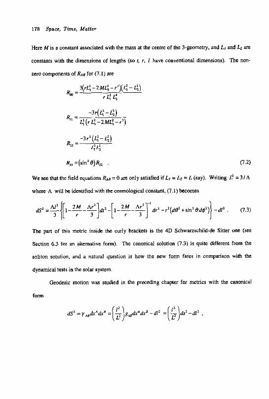
178 Space, Time, Matter
Hen M is a constant associated with the mass at the centre of the 3-geometry, and L, and LZ are
constants with the dimensions of lengths (so f, r, 1 have conventional dimensions). The non-
zero components of RAB for (7.1) are
qrg -ZMG - r 3 ) ( c - g ) r c L :
b =
- 3 r 2 ( c - 4 )
cc 4 2 =
R,, =(sin2 e)&2 . (7.2)
We see that the field equations RAE = 0 are only satisfied if LI = 152 = L (say). Writing L2 = 31 A
where A will be identified with the cosmological constant, (7.1) becomes
The part of this metric inside the curly brackets is the 4D Schwarzschild-de Sitter one (see
Section 6.3 for an alternative form). The canonical solution (7.3) is quite different from the
soliton solution, and a natural question is how the new form fares in comparison with the
dynamical tests in the solar system.
Geodesic motion was studied in the preceding chapter for metrics with the canonical
form
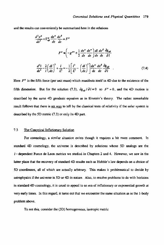
Canonical Solutions and Physical Quantities 179
and the results can conveniently be summarized here in the relations
(7.4)
Here F’ is the fifth force (per unit mass) which manifests itself in 4D due to the existence of the
fifth dimension. But for the solution (7.3), dg4 l d l = 0 so F” = 0, and the 4D motion is
described by the same 4D geodesic equation as in Einstein’s theory. The rather remarkable
result follows that there is to tell by the classical tests of relativity if the solar system is
described by the 5D metric (7.3) or only its 4D part.
7.3 Th e Canonical Inflationarv Solution
For cosmology, a similar situation exists though it requires a bit more comment. In
standard 4D cosmology, the universe is described by solutions whose 5D analogs are the
1 -dependent Ponce de Leon metrics we studied in Chapters 2 and 4. However, we saw in the
latter place that the recovery of standard 4D results such as Hubble’s law depends on a choice of
5D coordinates, all of which are actually arbitrary. This makes it problematical to decide by
astrophysics if the universe is 5D or 4D in nature. Also, to resolve problems to do with horizons
in standard 4D cosmology, it is usual to appeal to an era of inflationary or exponential growth at
very early times. In this regard, it turns out that we encounter the same situation as in the 1-body
problem above.
To see this, consider the (3D) homogeneous, isotropic metric
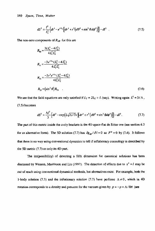
180 Space, Time, Matter
dS2 = - (d t2 -e”~[dr ’+r2 (dBZ 1’ +sin2Bd#2)]]-d12 . r: (7.5)
The non-zero components of RAB for this are
We see that the field equations are only satisfied if LI = 2L2 = L (say). Writing again L2 = 3 / A ,
(7.5) becomes
dS2 = ~ { d t 2 - e x p ( Z ~ t ~ d r ’ 3 +r1(dB2+sin2ed#*)]}-d1’. (7.7)
The part of this metric inside the curly brackets is the 4D space-flat de Sitter one (see section 6.3
for an alternative form). The 5D solution (7.7) has dg, l d l = 0 so F’ = 0 by (7.4). It follows
that there is no way using conventional dynamics to tell if inflationary cosmology is described by
the 5D metric (7.7) or only its 4D part.
The im(possibi1ity) of detecting a fifth dimension for canonical solutions has been
discussed by Wesson, Mashhoon and Liu (1997). The detection of effects due to x4 = I may be
out of reach using conventional dynamical methods, but alternatives exist. For example, both the
1-body solution (7.3) and the inflationary solution (7.7) have perforce A # 0 , which in 4D
notation corresponds to a density and pressure for the vacuum given by p = - p = A / 8~ (see
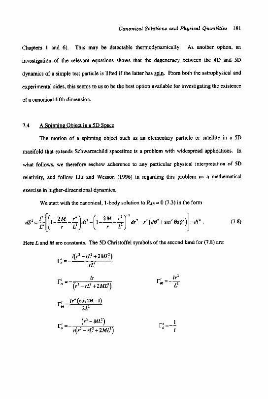
Canonical Solutions and Physical Quantities 181
Chapters 1 and 6). As another option, an
investigation of the relevant equations shows that the degeneracy between the 4D and 5D
dynamics of a simple test particle is lifted if the latter has @. From both the astrophysical and
experimental sides, this seems to us to be the best option available for investigating the existence
of a canonical fifth dimension.
This may be detectable thermodynamically.
7.4 ASo inninn Obiect in a 5D $Dace
The motion of a spinning object such as an elementary particle or satellite in a 5D
manifold that extends Schwarzschild spacetime is a problem with widespread applications. In
what follows, we therefore eschew adherence to any particular physical interpretation of 5D
relativity, and follow Liu and Wesson (1996) in regarding this problem as a mathematical
exercise in higher-dimensional dynamics.
We start with the canonical, 1-body solution to RAB = 0 (7.3) in the form
dSz = $[ (1 - 2 M - ~ ) d f ‘ r2 -( 1 -r 2 M - F) r2 -’ dr2 - r2 (do2 +sinz edg’)
Here Land M are constants. The 5D Christoffel symbols of the second kind for (7.8) are:
- rL2 + ~ M L ’ ) r,: =- r~~
(r’ - ML’) r;=- r(r3 - r ~ 2 + ~ M L ~ )
(7.8)
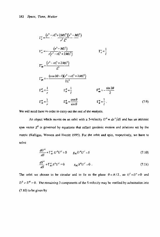
182 Space, Time, Matter
( r3 - rL*+ ~ M L ’ ) ( r3 - ML’) r3 L‘
r,; =
(r’ - ML’) r ( r3 -rLz + ~ M L ’ )
r,: =-
( r3 -rL2 + ~ M L ’ ) L’
r; =
(COS 28 - 1)( r3 - rL’ + 2 ~ 4 ~ ’ )
2 LZ r;o =-
re-- 1 w - l
cos 8 relp =- sin 8
sin 2 8 re +#- 2
1 r; = i (7.9)
We will need these in order to carry out the rest of the analysis.
An object which moves on an orbit with a 5-velocity U A = drA/dS and has an intrinsic
spin vector 9 is governed by equations that reflect geodesic motion and relations set by the
metric (Kalligas, Wesson and Everitt 1995). For the orbit and spin, respectively, we have to
solve
(7.10) dUA dS
dS A
dS
-+r;cuBuc=o gBcuBuc=i
-++;csRuc =o gBCsBuc =o . (7.11)
The orbit we choose to be circular and to lie in the plane 8 = n / 2 , so U’=U‘=O and
U z = Ua = 0. The remaining 3 components of the 5-velocity may be verified by substitution into
(7.10) to be given by
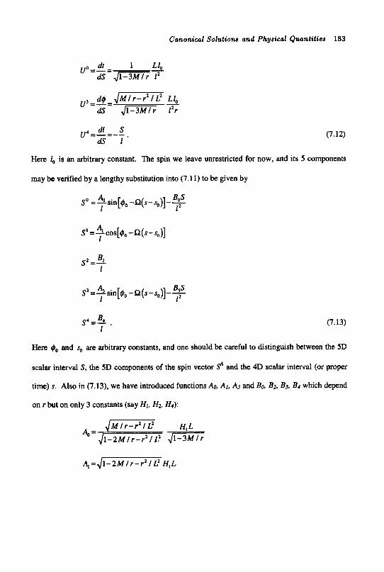
Canonical Solutions and Physical Quantities 183
(7.12)
Here lo is an arbitrary constant. The spin we leave unrestricted for now, and its 5 components
may be verified by a lengthy substitution into (7.1 1) to be given by
SO =-sin[$, 4 - ~ ( s - so)]- A B S 1 f Z
s ~ = ~ c o s [ 9 0 - s l ( s - s o ) ] 1
Here 4, and so are arbitrary constants, and one should be careful to distinguish between the 5D
scalar interval S, the 5D components of the spin vector 9 and the 4D scalar interval (or proper
time) s. Also in (7.13), we have introduced functions Ao, A], A3 and Bo, B2. B3, B4 which depend
on r but on only 3 constants (say HI, H2, H4):
4- H , L '= ~ 1 - 2M 1 r-rz 1 L2 ,/-
A, =$- 2 M I r - r2 I L1 H , L
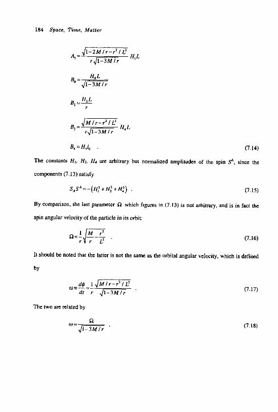
184 Space, Time, Matter
1 - 3 M l r
B4 = HJ0 . (7.14)
The constants HI, H2, H d are arbitrary but normalized amplitudes of the spin 9, since the
components (7.13) satisfy
S,S A = - ( H ; + H,' + H;) . (7.15)
By comparison, the last parameter C.3 which figures in (7.13) is not arbitrary, and is in fact the
spin angular velocity of the particle in its orbit:
p=- (7.16)
It should be noted that the latter is not the same as the orbital angular velocity, which is defined
by
The two are related by
(7.17)
51 '
(7.18)
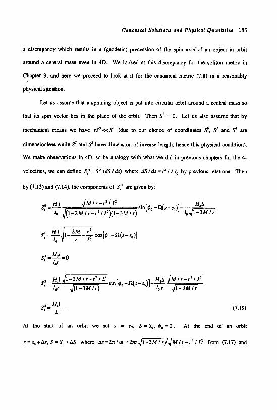
Canonical Solutions and Physical Quantities 185
a discrepancy which results in a (geodetic) precession of the spin axis of an object in orbit
around a central mass even in 4D. We looked at this discrepancy for the soliton metric in
Chapter 3, and here we proceed to look at it for the canonical metric (7.8) in a reasonably
physical situation.
Let us assume that a spinning object is put into circular orbit around a central mass so
that its spin vector lies in the plane of the orbit. Then 9 = 0. Let us also assume that by
mechanical means we have rS3<<S' (due to our choice of coordinates 9, S' and s' are
dimensionless while 9 and 9 have dimension of inverse length, hence this physical condition).
We make observations in 4D, so by analogy with what we did in previous chapters for the 4-
velocitiea, we can define S: = S A (dS I ds) where dS Ids = I* I Ll,, by previous relations. Then
by (7.13) and (7.14), the components of S: are given by:
H4S -iJT?zz sin [40 -a( s- so)] - 8," =3! JzZz
10 F G l L2)(1-3Mlr)
H,I 4 - 2 M f r - r 2 I L2 H,S ,/- lor .= lor -JTZFT sj =- sin[go - ~ ( s - so)]--
(7.19)
At the start of an orbit we set s = SO, S=So, go = O . At the end of an orbit
s=so+As,S=So+AS where A s = 2 z l u = 2 m , / ~ / ~ ~ from (7.17) and
186 Space, T i m e , Matter
AS = ( l z I Ll,)hs from above. The angle $J does not go exactly to 271, but by analogy with the
4D problem has an offset &$ = rAS: IS: where AS: E S:(s)-Sr’(so). These relations combined
with (7.19) in the weak-field approximation (r2 / Lz << M / r<< l ) give the precession angle for
one orbit, and the effect will accumulate over the 1 / LLTE ,/=’ orbits in a year (Liu and
Wesson 1996). For an experiment of short duration (As << L), the expression for the precession
per orbit is fairly simple:
(7.20)
This is the analog of (3.66) for the soliton metric (3.4). but now for the different 1-body
canonical metric (7.8). The first term in (7.20) is the usual geodetic precession found in 4D
general relativity. The second term will be small because it depends on the (presumably
cosmological) length L in the metric. However, the terms in (7.20) depend quite differently on
the radial distance r, so in principle they could be separated. In fact, the conditions we have used
to derive (7.20) might be realized in an Earthlartificial satellite situation as envisaged in the GP-
B project (see Jantzen, Keiser and Ruffini 1996). Alternatively, the conditions we have used are
close to those in the SudUranus situation. In these and other situations, it is in principle possible
to differentiate between 4D and 5D manifolds by measuring the contribution to the precession in
4D due to spin in the fifth dimension.
7.5 The Nature of Mass and Charge
It is widely acknowledged that the best way to test classical field theories of gravity and
electromagnetism is through the dynamics of a test particle of rest mass rn and charge q. This
view has some historical justification insofar as it validates general relativity and classical
Canonical Solutions and Physical Quantities 187
electromagnetism. But it is flawed, because in both theories there is no physical explanation for
m and q on the same basis as there is for the other quantities which appear in the equations. This
problem was mentioned in Chapter 1 , and there have been several notable attempts to tackle it
(Jammer 1961; Hoyle and Narlikar 1974; Barbour and Pfister 1995). A partial resolution was
obtained in Chapter 5, where we used the 4D part of the 5D geodesic equation to give a
geometrical interpretation for the ratio q/m. We now wish to revisit this problem from a different
angle (Wesson and Liu 1997), and use the canonical metric to offer a complete explanation of
charge and mass.
Let us start by reconsidering dynamics in 4D and 5D, assuming that the former has to be
embedded in the latter, but using only the metric and neglecting constraints that might derive
from a set of field equations.
In 4D, we have a line element which is given in terms of a metric tensor by
dr2 =g4 h a d r e , and a Lagrangian which is commonly defined as
ak dr' L=m--+q A,, - dA dA
(7.21)
Here h is a parameter and A, is the electromagnetic potential. This is acceptable, but clearly rn
and q are introduced ad. Overlooking this for the moment, we form the momentum 4-vector
(7.22)
That is, pa =mgd up +q& and p a I g d p p = mua +qAa where ua = ha Ids is the 4-velocity.
The product is
papa =m2uaua+2mq&ua+q'&Aa , (7.23)
188 Space, T i m e , Matter
which is just +mz when we choose the signature to be g,=(+l,-l,-l,-l) and put q = 0.
Locally g+ 5 q+, and for a charged particle moving with a 3-velocity v ' * ~ = d ~ ' * ~ / d t we have
p o =m-+qAO=--- dr m 112 + 4 A0
ds ( 1 4 )
dr12' mvl" p"' = m-+qA'2' =- I,' +qA"' , ds (1 - v')
(7.24)
(7.25)
which we call the energy and (3D) momenta. These relations lead of course to the result
E 2 = p*+m' , which is the basis of particle physics and is in excellent agreement with
experimental data. However, as pointed out above, there is no explanation of m or (if it is finite)
of q.
In 5D, we have a line element which is given in terms of a metric tensor by
aS2 = g,,drAdra and which as in Chapter 5 we can rewrite as the sum of a 4D part and an extra
part that depends on scalar and vector fields:
dS2 =g,dr"dxa -@'(dl +Audxu)* .
The corresponding Lagrangian is
(7.26)
(7.27)
Here m is still introduced adhoc, but the theory has one extra parameter associated with the fifth
coordinate 1 and the charge q does not appear explicitly (see below). From (7.27) we can form
the 4-part of the momentum 5-vector:
Canonical Solutions and Physical Quantities 189
(7.28)
This is the 5D analog of the 4D relation (7.22). The extra or fifth component is
< = m n . (7.29)
We see that the scalar function n of (7.28) specifies the momentum in the extra dimension (see
Chapters 1 and 5). We might expect n to be small in many situations, because from (7.26) and
(7.28) we have dsldS=(l+n21@2)112 as in (5.22), so ds sds in this case. To get the
contravariant forms of the covariant vectors (7.28) and (7.29), we note that
(7.30)
with A' i gpv&. This gives Pa = gd PB = m Ua and P' = g"PB = mU4 where U" = hA I dS
is the 5-velocity. The product is
pApA = m2 . (7.31)
This is the 5D analog of the 4D relation (7.23). However, q does not appear in the former
whereas it does in the latter, so we need to inquire where this parameter fits into the extended
geometry. To answer this, we rewrite (7.28) as
P, =rn[gMUB+nAa] . (7.32)
Although it is the 4-part of a 5-vector, the metric (7.26) from which it is derived is invariant
under the 4D subset of general 5D coordinate transformations xa + x" ( x s ) , and so therefore
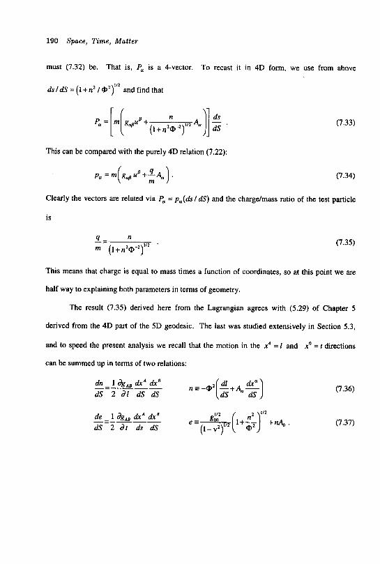
190 Space, Time, Matter
must (7.32) be. That is, Pa is a 4-vector. To recast it in 4D form, we use from above
d s / d S = ( l + n 2 / @ 2 ) 1 1 2 andfindthat
(7.33)
This can be compared with the purely 4D relation (7.22):
pa = m ( g @ u f i + t % ) (7.34)
Clearly the vectors are related via Pa = p a ( d s / d S ) and the chargdmass ratio of the test particle
is
(7.35)
This means that charge is equal to mass times a function of coordinates, so at this point we are
half way to explaining both parameters in terms of geometry.
The result (7.35) derived here from the Lagrangian agrees with (5.29) of Chapter 5
derived from the 4D part of the 5D geodesic. The last was studied extensively in Section 5.3,
and to speed the present analysis we recall that the motion in the x4 = 1 and xo = t directions
can be summed up in terms of two relations:
dn - 1 dg,, d x A dr8 dS 2 d l dS dS n = -oz( $+& s)
112 de - 1 dgAB dx" dx' e =A( I12 $) 1+- +&.
dS 2 d t ds dS (1 - vz)1/2
(7.36)
(7.37)
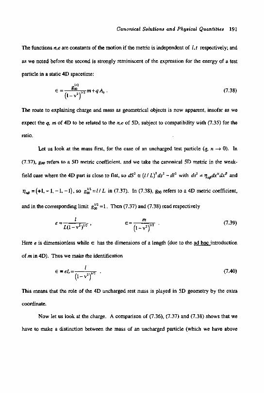
Canonical Solutions and Physical Quantit ies 191
The functions n,e are constants of the motion if the metric is independent of 1,t respectively; and
as we noted before the second is strongly reminiscent of the expression for the energy of a test
particle in a static 4D spacetime:
(7.38)
The route to explaining charge and mass as geometrical objects is now apparent, insofar as we
expect the q, m of 4D to be related to the n,e of 5D, subject to compatibility with (7.35) for the
ratio.
Let us look at the mass first, for the case of an uncharged test particle (9, n -) 0). In
(7.37). goo refers to a 5D metric coefficient, and we take the canonical 5D metric in the weak-
field case where the 4D part is close to flat, so dS2 I ( I / L)'ds2 - d12 with ds2 = %,,dradxa and
112 - vM = (+I, - 1, - 1, - 1), so g, -1 / I, in (7.37). In (7.38), goo refers to a 4D metric coefficient,
and in the corresponding limit g t = I . Then (7.37) and (7.38) read respectively
(7.39)
Here e is dimensionless while E has the dimensions of a length (due to the ad hoc introduction
of m in 4D). Thus we make the identification
(7.40)
This means that the role of the 4D uncharged rest mass is played in 5D geometry by the extra
coordinate.
Now let us look at the charge. A comparison of (7.36), (7.37) and (7.38) shows that we
have to make a distinction between the mass of an uncharged particle (which we have above
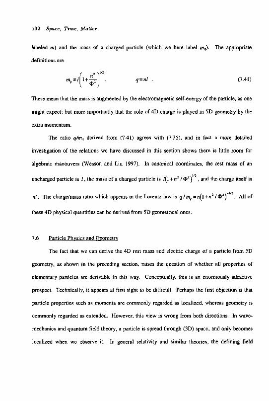
192 Space, Time, Matter
labeled m) and the mass of a charged particle (which we here label mq). The appropriate
definitions are
m 4 a1 ( 1 + ~ $)”’ , q=nl (7.41)
These mean that the mass is augmented by the electromagnetic self-energy of the particle, as one
might expect; but more importantly that the role of 4D charge is played in 5D geometry by the
extra momentum.
The ratio q/mq derived from (7.41) agrees with (7.33, and in fact a more detailed
investigation of the relations we have discussed in this section shows there is little room for
algebraic manouvers (Wesson and Liu 1997). In canonical coordinates, the rest mass of an
uncharged particle is 1 , the mass of a charged particle is l(1 + n 2 /@z)”2 , and the charge itself is
n l . The charge/mass ratio which appears in the Lorentz law is q / m S = n ( l + n 2 /@’)-’’’. All of
these 4D physical quantities can be derived from 5D geometrical ones.
7.6 Particle Physics and Geometry
The fact that we can derive the 4D rest mass and electric charge of a particle from 5D
geometry, as shown in the preceding section, raises the question of whether all properties of
elementary particles are derivable in this way. Conceptually, this is an enormously attractive
prospect. Technically, it appears at first sight to be difficult. Perhaps the first objection is that
particle properties such as momenta are commonly regarded as localized, whereas geometry is
commonly regarded as extended. However, this view is wrong from both directions. In wave-
mechanics and quantum field theory, a particle is spread through (3D) space, and only becomes
localized when we observe it. In general relativity and similar theories, the defining field
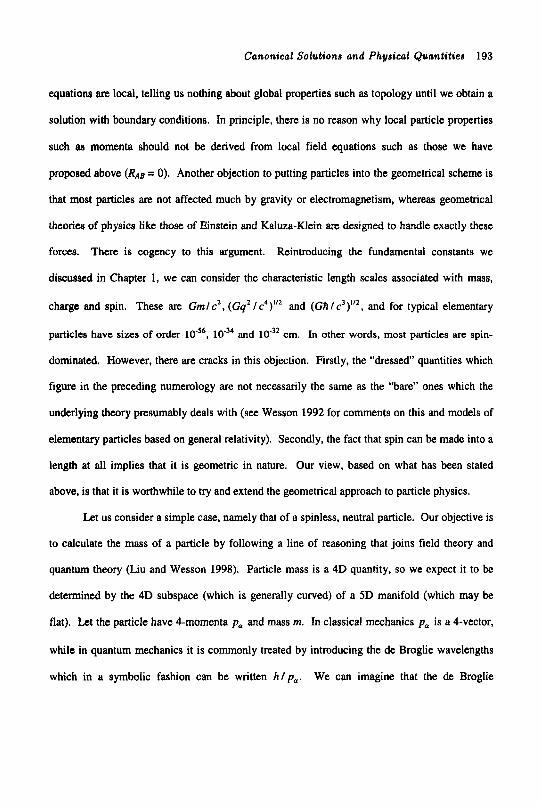
Canonical Solutions and Physical Quantities 193
equation8 are local, telling us nothing about global properties such as topology until we obtain a
solution with boundary conditions. In principle, there is no reason why local particle properties
such aa momenta should not be derived from local field equations such as those we have
proposed above (RAB = 0). Another objection to putting particles into the geometrical scheme is
that most particles are not affected much by gravity or electromagnetism, whereas geometrical
theories of physics like those of Einstein and Kaluza-Klein are designed to handle exactly these
forces. There is cogency to this argument. Reintroducing the fundamental constants we
discussed in Chapter 1, we can consider the characteristic length scales associated with mass,
charge and spin. These are Gmlc’, (Gq’ Ic‘)”’ and (GAIC’) ’ ’~ , and for typical elementary
particles have sizes of order and cm. In other words, most particles are spin-
dominated. However, there are cracks in this objection. Firstly, the “dressed” quantities which
figure in the preceding numerology are not necessarily the same as the “bare” ones which the
underlying theory presumably deals with (see Wesson 1992 for comments on this and models of
elementary particles based on general relativity). Secondly, the fact that spin can be made into a
length at all implies that it is geometric in nature. Our view, based on what has been stated
above, is that it is worthwhile to try and extend the geometrical approach to particle physics.
Let us consider a simple case, namely that of a spinless, neutral particle. Our objective is
to calculate the mass of a particle by following a line of reasoning that joins field theory and
quantum theory (Liu and Wesson 1998). Particle mass is a 4D quantity, so we expect it to be
determined by the 4D subspace (which is generally curved) of a 5D manifold (which may be
flat). Let the particle have 4-momenta p, and mass m. In classical mechanics pa is a 4-vector,
while in quantum mechanics it is commonly treated by introducing the de Broglie wavelengths
which in a symbolic fashion can be written hip, . We can imagine that the de Broglie
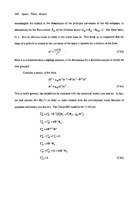
194 Space, Time, Matter
wavelengths are related to the dimensions of the principle curvatures of the 4D subspace, or
alternatively to the Ricci tensor R$ or the Einstein tensor GOs 3 R, - Rg+ I 2 . For these latter,
G = - R is an obvious scalar to relate to the scalar mass m. This leads us to conjecture that the
mass of a particle is related to the curvature of the space it inhabits by a relation of the form
(7.42) k h 2 R ,2=- .
C2
Here k is a dimensionless coupling constant, to be determined by a detailed analysis to which we
now proceed.
Consider a metric of the form
dS2 = gA,drAdXS = 0 2 d s 2 - OZbdl2
ds2=g,dradrB . (7.43)
This is fairly general, but should not be confused with the canonical metric (see above). In fact,
we will assume @ = O(x") in order to make contact with the conventional wave function of
quantum mechanics (see below). The Christoffel symbols for (7.43) are
f-; =r; +~-~(s;o, +s;~, -gSyOa)
f-; = r; +4@-l@,
r; = & o ~ ~ - ~ @ ~
p = r 4 -r4 -
I-':" = bO%,
0 4 o$- 44-0
I-'; = r; + ( b + 4 ) w 1 0 a
r& =o (7.44)
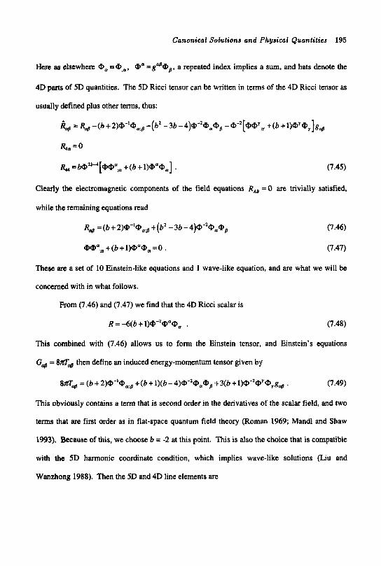
Canonical Solution8 and Physical Quantities 195
Hen 89 elsewhere 0, SQ,,, 0" =g@@,, a repeated index implies a sum, and hats denote the
4D parts of 5D quantities. The 5D Ricci tensor can be written in terms of the 4D Ricci tensor as
usually defined plus other terms, thus:
& = R4-(b+2)@-'@,; , -(bz -36-4)@-*0,#, -@-2[@@r;y +(b+l)@'#,]g,
R,, =O
& = b P - 4 [ 0 @ a ; , +(b+l)0"0,] . (7.45)
Clearly the electromagnetic components of the field equations R , = 0 are trivially satisfied,
while the remaining equations read
RM =(b+2)@-'0, , +(b' -3b-4)0-*@,0, (7.46)
(7.47)
These are a set of 10 Einstein-like equations and 1 wave-like equation, and are what we will be
concerned with in what follows.
mop +(b + l)O"On =O .
From (7.46) and (7.47) we find that the 4D Ricci scalar is
R = -6(b t l)@-2@a@a . (7.48)
This combined with (7.46) allows us to form the Einstein tensor, and Einstein's equations
GopB = 8HM then define an induced energy-momentum tensor given by
8 f l , = ( b + 2 ) 0 - ' 0 , ; , +(b+l)(b-4)0"@,0, +3(b+l)0-Z0'0,g, . (7.49)
This obviously contains a term that is second order in the derivatives of the scalar field, and two
terns that m first order as in flat-space quantum field theory (Roman 1969; Mandl and Shaw
1993). Because of this, we choose b = -2 at this point. This is also the choice that is compatible
with the 5D harmonic coordinate condition, which implies wave-like solutions (Liu and
Wanzhong 1988). Then the 5D and 4D line elements are
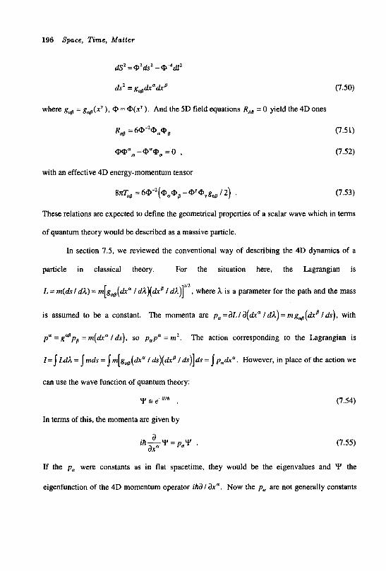
196 Space, T i m e , Matter
dS2 =02dS2 -Q4d12
ds2 = g,akaaka (7.50)
where g, = g4(xy), Q, = Q , ( x y ) . And the 5D field equations RAB = 0 yield the 4D ones
R, = 6@-20a@a (7.51)
= 0 , (7.52)
with an effective 4D energy-momentum tensor
BH, = 6@-2(@a@,, - OYQ,,.g, / 2) . (7.53)
These relations are expected to define the geometrical properties of a scalar wave which in terms
of quantum theory would be described as a massive particle.
In section 7.5, we reviewed the conventional way of describing the 4D dynamics of a
particle in classical theory. For the situation here, the Lagrangian is
L = m(ds/dd) = rn[g,(aka ldd)(aka /dd)]"2, where h is a parameter for the path and the mass
is assumed to be a constant. The momenta are pa =aLla(dxa l d d ) = mg,(dra Ids), with
p a = g@pa = m ( h a Ids) , so papu = m2. The action corresponding to the Lagrangian is
Z=jL,dd=jrnds=jrn[g,(dx" / d s ) ( h a Ids) ]ds=jpaaka. However, in place of the action we
can use the wave function of quantum theory:
y e-i/!h
In terms of this, the momenta are given by
a ax. ih--Y = p a y
(7.54)
(7.55)
If the pa were constants as in flat spacetime, they would be the eigenvalues and Y the
eigenfunction of the 4D momentum operator ihd I axa. Now the pa are not generally constants
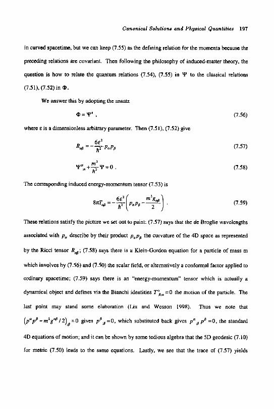
Canonical Solutions and Physical Quantities 197
in curved spacetime, but we can keep (7.55) as the defining relation for the momenta because the
preceding relations are covariant. Then following the philosophy of induced-matter theory, the
question is how to relate the quantum relations (7.54), (7.55) in Y to the classical relations
(7.51), (7.52) in a. We answer this by adopting the ansatz
@ = Y e , (7.56)
where E is a dimensionless arbitrary parameter. Then (7.51). (7.52) give
m2 YUu+-Y=O
A=
The corresponding induced energy-momentum tensor (7.53) is
(7.57)
(7.58)
(7.59)
These relations satisfy the picture we set out to paint: (7.57) says that the de Broglie wavelengths
associated with pa describe by their product popB the curvature of the 4D space as represented
by the Ricci tensor Re; (7.58) says there is a Klein-Gordon equation for a particle of mass rn
which involves by (7.56) and (7.50) the scalar field, or alternatively a conformal factor applied to
ordinary spacetime; (7.59) says there is an “energy-momentum” tensor which is actually a
dynamical object and defines via the Bianchi identities T>;u =O the motion of the particle. The
last point may stand some elaboration (Liu and Wesson 1998). Thus we note that
( p a p B -m2ge / 2 ) ,p=0 gives P ~ ; ~ = O , which substituted back gives p a i p p B =0, the standard
4D equations of motion; and it can be shown by some tedious algebra that the 5D geodesic (7.10)
for metric (7.50) leads to the same equations. Lastly, we see that the trace of (7.57) yields
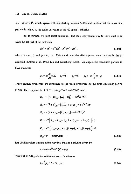
198 Space, Time, Matter
R=-6&’mZ I h 2 , which agrees with our starting relation (7.42) and implies that the mass of a
particle is related to the scalar curvature of the 4D space it inhabits.
To go further, we need exact solutions. The most convenient way to show such is to
write the 4D part of the metric as
ds2 = dt2 - e2’& - e2’dy2 - dZZ , (7.60)
where a = k(t,z) and p = p(t,z). This metric can describe a plane wave moving in the z-
direction (Kramer et al. 1980; Liu and Wanzhong 1988). We expect the associated particle to
have momenta
(7.61) dz dt ds ds
pi =0, p, =0, p3 = - m - = - p po = rn-= E,
These particle properties are connected to the wave properties by the field equations (7.57),
(7.58). The components of (7.57), using (7.60) and (7.61), read
R , , , , = - ( A + p ) , , - ( A ~ o + + ~ ) = - 6 ~ Z A ~ 2 E Z
%I =-(a+P),O1 -(4041 +P,oP,1)= 6E2h-,EP
R~~ =-(a + p),]] -(a:3 + p:)= - 6 ~ ~ h - ~ ~ ~
RiI = e Z ’ [ [ i l , ~ - a , 1 3 t a , O ~ a ~ ~ ~ , ~ ~ a , l ~ a ~ ~ ~ , ~ ] ~ o
4 2 =ezp [Pm -P,11 + P , o ( ~ + P ) , o - P , l ( ~ + P ) , l ] = o
R@=O (otherwise) .
It is obvious when written in this way that there is a solution given by
a=-p=&&-i(Et-pz).
This with (7.54) gives the action and wave function as
I = p&” = Et - pz
(7.62)
(7.63)
(7.64)

Canonical Solutions and Physical Quantities 199
= e - m - ~ ~ ) / n (7.65)
The last should satisfy the fifth or Klein-Gordon part of the field equations (7.58), and we find
that it does so. The induced or effective 4D energy-momentum tensor by (7.59) and (7.61) has
the following nonzero components:
87t" = - 6.s2h-'( E' - m2 / 2 )
8H;O =-q'=6&2h-ZEp
SnT,' = T,' = 3 ~ ~ A - ~ m ~
8 7 L 5 ~ = 6 ~ . ~ h - ' ( p ~ + r n ~ / 2 ) . (7.66)
These obey 8Z7" = 6 ~ ~ A - ~ r n ~ , and we recall that E, p, m are related by pupu = EZ - p 2 =m2. This
constraint means that we have a class of exact solutions that depends on 2 independent
dpamical constants, E and p. [The dimensionless constant E which we introduced in (7.56) to
connect the scalar field potential and the wave function could in principle be absorbed into E and
p . or into A .] We can sum up the 5D wave solution as follows:
=y2'&2 -y"ed12 (7.67)
h2 =dt2 -elA& -e-2Adyz -dzz (7.68)
y=e-'(fl-Pz)'', a = J S d i - l ( ~ ~ - ~ ~ ) . (7.69)
We have examined algebraic properties of this class of solutions using a fast software package.
Apart from confirming RAB = 0, we find RABCD f 0 so these solutions are not 4D curved and 5D
flat like those considered in Section 4.7 (for example, for the above solutions we find that
R,,', = -2e2(3E2 +pz)Y"' t O and K = RAscDRABCD z0) . However, while these solutions are in
general curved, they have f i = l for the determinant of the 4D metric and so are special
algebraically.
200 Space, Tame, Matter
This last point, plus other choices we have made along the way, leave broad scope for a
more general examination of the idea that particle rest mass is related to spacetime curvature. We
finish this section by focussing on two issues that need to be examined before such a Machian
view can be adopted. First, it is not always possible to write the Ricci tensor as the product of
two (momentum) vectors, as in (7.57). More work is needed on this presumably using the Segre
classification of the Ricci tensor (Paiva, Reboucas and Teixeira 1997). Second, it is possible to
change the conformal factor on the 4D spacetime part of a 5D metric (7.43). which changes the
mass as defined by (7.42). For example, consider two 4D metrics related by a conformal
transformation, g4 =enCx)gM, with Ricci scalars R and Ti (Synge 1960). Then
(7.70)
This means in the induced-matter picture that a massless particle (R=O) becomes massive
(R#O) by virtue of a conformal transformation of the 4D metric. In other words, conformal
transformations in classical field theory are the analog of the Higgs mechanism in quantum
theory.
7.7 Conclusion
The canonical coordinate system for 5D metrics leads to major physical insights. The 1-
body solution (7.1) involves no departure from conventional dynamics, so from the classical tests
in the solar system there is no way to tell if we should use the 5D metric or only its 4D part. The
inflationary cosmological solution (7.7) leads to the same conclusion. But in both cases, the
metric only exists if there is a finite cosmological constant, or equivalently a finite energy
density for the vacuum; so in principle a way to differentiate between 5D and 4D is to use
thermodynamics. Another way is to use a spinning object, since the equations (7.10), (7.11)
Canonical Solutions and Physical Quantities 201
which govern this effectively lift degeneracy, and result in a precession formula (7.20) which
picks up a term from the fifth dimension.
In the canonical frame, a comparison of 4D and 5D dynamics shows that the momenta of
particles are simply related by the ratio of the intervals, and that the chargdmass ratio of a
particle (7.35) follows from this and is geometrical in nature. A closer examination shows that
the mass or energy of an uncharged particle (7.40) is just x4=1 , and that the electric charge
(7.41) is just a multiple of this. In other words, in the canonical frame, mass is a coordinate and
charge is a momentum.
However, all coordinate frames are valid in 5D relativity, so the question arises of how to
define the mass of a particle in a general, non-canonical, frame. Following the induced-matter
philosophy, it is reasonable to suppose that the momenta of a particle, or its de Broglie
wavelengths, are related to the principal curvatures of the 4D subspace it inhabits; and that its
mass is related to the scalar curvature of that subspace. The latter condition is easier to quantify
as in (7.42). which says that the mass (squared) is proportional to the Ricci scalar. The former
condition is harder to quantify, but as in (7.57) implies a relation between the momenta
(producted) and the Ricci tensor. We obviously need more work on this, especially on how the
conformal factor for the 4D space affects the Ricci scalar (7.70) and thereby the mass. However,
the results of Section 7.6 for particles run parallel to those of Section 4.4, which showed the
existence of classical vacuum waves with complex metric coefficients. Then a reasonable
inference is that the wave function of quantum theory is related to a complex conformal function
applied to classical spacetime.
202 Space, Time, Matter
References (ChaDter 7)
Barbour, J.B., Pfister, H. (eds.) 1995, Mach’s Principle: From Newton’s Bucket to Quantum
Gravity (Birkhauser, Boston).
Hoyle, F., Narlikar, J.V. 1974, Action at a Distance in Physics and Cosmology (Freeman, San
Francisco).
Jammer, M. 1961, Concepts of Mass in Classical and Modem Physics (Harvard U. Press,
Cambridge).
Jantzen, R.T., Keiser, G.M., Ruffini R. (eds.) 1996, Proc. 7th Marcel Grossman Meeting (World
Scientific, Singapore).
Kalligas, D., Wesson, P.S., Everitt, C.W.F. 1995, Astrophys. J. 439,548.
Gamer, D., Stephani, H., Herlt, E., MacCallum, M., Schmutzer, E. 1980, Exact Solutions of
Einstein’s Field Equations (Cambridge U. Press, Cambridge).
Liu, H., Wanzhong, S. 1988, Gen. Rel. Grav. 20,407.
Liu, H., Wesson, P.S. 1996, Class. Quant. Grav. 13,2311.
Liu, H., Wesson, P.S. 1998, Int. J. Mod. Phys. D 2,737.
Mandl, F., Shaw, G. 1993, Quantum Field Theory (Wiley, New York), 29.
Paiva, F.M., Reboucas. M.J., Teixeira, A.F.F. 1997, J. Math. Phys. 3,4228.
Roman, P. 1969, Introduction to Quantum Field Theory (Wiley, New York), 19.
Synge, J.L. 1960, Relativity: The General Theory (North Holland, Amsterdam), 318.
Wesson, P.S. 1992, Space Sci. Rev. 3,365.
Wesson, P.S., Liu, H. 1997, Int. J. Theor. Phys. 36, 1865.
Wesson, P.S., Mashhoon, B., Liu, H. 1997, Mod. Phys. Lett A 12,2309.
8. RETROSPECT AND PROSPECT
'To put the conclusion crudely - the stuff of the world is mind-stuff'
(Sir AS. Eddington, Cambridge, 1939)
By this quote, Eddington did not mean that we create the world inside our heads. He
rather meant that we perceive an external world, but strongly influenced by the physiological and
psychological constraints that attach to us being human. This view was one he was led to after
experiencing and pattaking in the development of relativity and quantum theory in the first half
of the twentieth century. More recent developments, including the ones outlined in this book,
bolster the view that physics is not discovered so much as invented.
In Chapter 1, we saw that fundamental constants can be brought into and removed from
physics as a matter of convenience. In Chapter 2, Riemannian geometry in 5D was used to
remove the artificial distinction between the field and its source: what we call matter is, at least
at the classical level. the result of geometry. This induced-matter theory uses the field equations
RAB(x') = 0, and is algebraically much richer than old Kaluza-Klein theory with
CAB(xa) = 8flm(x") or Einstein's theory with G,(xy) = 8flM(xy) . But it contains general
relativity, and as shown in Chapter 3 the 1-body soliton solutions agree with the classical tests.
In Chapter 4, we used exact solutions of RAB = 0 with their associated T,(xA) to examine a
number of systems of cosmological and astrophysical importance. The standard 4D cosmology,
consisting of the radiation-dominated solution for early times and the dust (Einstein-de Sitter)
solution for late times, is curved in 4D but flat in 5D. Mathematically, we have to conclude that
the 4D big bang is due to an unfortunate choice of 5D coordinates. Conceptually, it is subjective
or invented in the Eddingtonian sense. Electromagnetism was treated in Chapter 5 as in the
203
204 Space, Time, Matter
original theory of Kaluza, and charged solitons and black holes if they should be detected
astrophysically would differentiate between 4D and 5D. In Chapter 6, the idea of a canonical
metric was introduced. While natural, this has radical implications: the world model does not
exist unless there is a fifth dimension, and if the 4D part of the model depends on the extra
coordinate there exists a fifth force. The ramifications of the canonical metric were examined in
Chapter 7. There is a 1-body class of solutions which “intersects” the soliton solutions insofar as
both classes contain the unique 4D Schwarzschild solution. For such solutions, we cannot tell if
the world is 5D or 4D merely by looking at conventional dynamics, but other effects including
spin can show the difference. The canonical scheme can be extended to particle physics, and
perhaps its most remarkable implication concerns the rest mass of a particle: there is at least one
coordinate system where the extra coordinate plays the role of mass.
However, the unification of space, time and matter we have outlined in the preceding
chapters leads to some questions:
(a) Is there anything special about 5D Riemannian space? The answer is almost
certainly, NO. To a first approximation, the world locally is 1D in nature ( x ’ > > x ’ * ~ ) . To a
better approximation it is described by 4D spacetime. Classical matter in spacetime can be
accommodated by a 5D manifold. But while ND Riemannian spaces have special algebraic
properties for small N , there is no reason to believe that there is some unique or chosen value for
it. We choose N in accordance with what physics we wish to explain. (This argument also
applies to N = 10, 11 as in superstrings and supergravity.) Indeed, we might wish to consider
N + - . A related possibility is that we may wish to go beyond symmetric Riemannian space to
consider non-symmetric spaces or ones with torsion, or more general spaces like that of Finsler,
all of which offer more algebraic opportunities that might be utilized for physics.
Retroscpect and Prospect 205
(b) The problem of zero-point fields in particle physics may be solved by
supersymmetry; and the equivalent (cosmological constant) problem in general relativity may be
solved by a scalar field. But more work is needed on the connection between these approaches.
In a classical 5D field theory like the one developed above, canonical metrics necessarily have a
parameter that plays the role of a 4D cosmological constant, so there is equivalently a vacuum
energy. However, if we adhere to the philosophy of Einstein, such properties of the vacuum are
the result of coordinate choices, and should not be elevated to any higher status (as done, for
example, in the theory of quantum electrodynamic vacuum polarization). We do not know how
many scalar fields, or equivalently what number of dimensions, are necessary to resolve these
problems with energy.
(c) The canonical 1-body solution is quite different from the soliton solution, and we
do not know which describes the field outside a massive object such as the Sun. We suspect that
it is the former, which implies some other physical identification for the solitons.
(d) In the canonical 5D metric. the extra coordinate plays the role of particle rest
mass. But the former can be negative, so can mass be negative also? The situation here is in
some ways analogous to the one encountered by Dirac when he was considering the theory of the
electron, and of course he was led to the proposal of the positron. In gravitational theory,
Bonnor has shown that there is nothing intrinsically contradictory about negative mass.
However, in a world where positive and negative mass both exist, the detection of an object with
negative mass would be problematical because it would repel other particles. Thus while 5D
theory naively predicts particles with negative mass, it is not clear how such particles could be
detected or why the world appears to consist predominantly of objects with positive mass.
206 Space, Time, Matter
(e) For canonical metrics whose 4D part depends on the extra coordinate, there is a
fifth force. Why has this hitherto escaped detection? A kind of answer to this can be given by
appeal to the weak equivalence principle, which implies that the 4D acceleration of a test particle
is independent of its mass. However, this really makes the equivalence principle a symmetry of
the metric, and does not yield a deeper explanation. A related question is why particle masses
appear (at least locally) to be constants, whereas the theory allows them to be variable. A
technical answer is that the coordinate system is one where the fifth component of the 5-velocity
is zero (i,e., x4 is comoving). However, this does not explain why 4D physics has evolved to use
masses as units.
(f) If a fifth force exists, it may only be apparent in microscopic systems, as opposed
to the macroscopic ones we have mainly considered in the preceding account. We can ponder
what the effects would be of 5D physics applied to elementary particles if we tried to interpret
the latter in 4D. (A different approach to this would be to reformulate quantum mechanics in
5D, which however we leave as an exercise for the reader.) To be specific: what would be the
effects of exact 5D conservation laws if we only considered their 4D parts? A possibility is that
effects commonly attributed to Heisenberg’s uncertainty principle in 4D could instead be
understood as the consequences of deterministic laws in 5D.
This last idea, while speculative, would have appealed to Einstein. He had the good
fortune (and skill) to succeed at most of the physics he took up. A lesson to be learned from his
work is that a powerful idea should be pushed forward; and it appears to us that the principle of
covariance is one of the most powerful ideas in modem physics. Field equations involving
tensors have enormous algebraic scope if we do not restrict the group of coordinate invariance
and do not restrict the number of dimensions. In 5D, we can realize Einstein’s vision of
Retroacpect and Prospect 207
transforming the “base-wood” of matter into the “marble” of geometry. The trick is simply to
keep the theory general algebraically and to make the appropriate identifications physically.
While we do not think it is the only way, we are led to the opinion that the world can be
described if we so choose in terms of pure geometry.
Axions 37 Axisymmetry 114
Big bang 49,100,126 Binary pulsar 105 Black holes 50,138,141 Brans-Dicke 32
Canonical gauge Charge (electric) COBE Coordinate changes Cosmological constant Cosmology (inflationary) Cosmology (standard) Covariance
158,204 11, 186,192 99 93,121,125.131 159,178, 180
111.179
44,92 104.165
Dark matter 96 D i m equation 21
Eddington 5, 37, 126,203 Einstein 1,37,206
Energy 136,190,199 Equivalence principle 81, 85, 124
Faraday tensor 19,31, 134 Fifth force 154,206 Flat metrics 117,170 Friedmann equations 15,94 Fundamental 2, 158, 193,203 constants
Embeddings 43
Gauges 154 General Relativity 11,85 Geodesic equation 17, 102, 132 Geodetic effect 82,186 GP-B 82, 186 Gravitinos 37
Harmonic gauge 155,195 Higgs mechanism 27,200 Horizons 16.50
Hubble’s law 104,179 Hoyle 195
Induced matter Inflation
JIM2 relation
Kaluza-Klein theory Klein-Gordon equation Kretschmann scalar
Light deflection
Mach’s principle Mass
Maxwell’s equations Membranes Microwave background
Neutrinos Nucleos ynthesis
Occam Orthogonality
Particles Prwa equation Pulsars
QSOs Quantum chromodynamics Quantum electrodynamics
Raychaudhuri equation Redshift effect Reissner-Nordstrom metric
Schrodinger equation Schwarzschild metric Shell metrics Solitons (charged) Solitons (static) Solitons (time- dependent) Spherical symmetry
42,206 111,179
10
28,203 21, 197 56,108,116,199
72,100
11, 176 10, 15, 105, 186, 193, 205 19,32,129 36 100
37 100
88 165, I72
18,192,196 23 88,105
88, 100 25
26
14 81 143
20 70, 124,142 117 138 49,69,96 111
105
208
209
Spin Standard model (cosmology) Standard model (particles) STEP Supersymmetry
Tensors Time
Units Uncertainty principle
Vacuum (4D) Vacuum (5D)
Wave metrics Weak interaction WIMPS
Yang-Mills theory
Zero-point fields
82,181,193 92
28
85 33,204,205
1 1 , 19,43,92,206 5.8.49, 104
7,193 206
13,93,159 30,49,93
108,199 27 37.96
24
93,161,205