Embed Size (px)
Citation preview

Space-Time Areal Mixture Model:
Relabeling Algorithm and Model Selection Issues
Md Monir Hossain, PhDMd Monir Hossain, PhD
Assistant Professor of Pediatrics
Division of Biostatistics and Epidemiology

Acknowledgement
Collaborator:
Andrew B Lawson (MUSC, Charleston)
Russell S Kirby (USF, Tampa)
Bo Cai (USC, Columbia)
Jihong Liu (USC, Columbia)
Jungsoon Choi (South Korea)Jungsoon Choi (South Korea)
NIH Grant:
NCI: R03 (08/06-08/08) (PI: Hossain)
NHLBI: R21 (06/09-04/12) (PI: Lawson, Cai, Hossain)
Earlier Works
Areal model (Stat in Med, 2006; EES, 2005):
Local-likelihood cluster (LLC) model
Compared with the BYM model
Results: For detecting clusters of low and medium risk areas,
LLC models signal better than BYM model
Cluster detection diagnostics Cluster detection diagnostics
Earlier Works
Spatio-temporal Areal model ((EES, 2012; EES, 2010) :
Space-time local-likelihood cluster (LLCST) model
Space-time mixture of Poisson (MPST) model
Space-time cluster detection diagnostics
Space-time stick-breaking process (SBPST)Space-time stick-breaking process (SBPST)
Compared with the SREST model
Motivation
With the growing popularity of using spatial mixture model in cluster
analysis, using model selection criteria to find the most
parsimonious model is an established technique.
Label-switching is an inherent problem with the mixture models and
a variety of relabeling algorithms have been proposed over the
decade.
We used a space-time mixture of Poisson regression model with
homogeneous covariate effects
The results are illustrated for real and simulated datasets.
The objective is to aware the researcher that if the purpose of
statistical modeling is to identify the clusters, applying the
relabeling algorithm to the best fitted model may not generate the
optimum labeling.
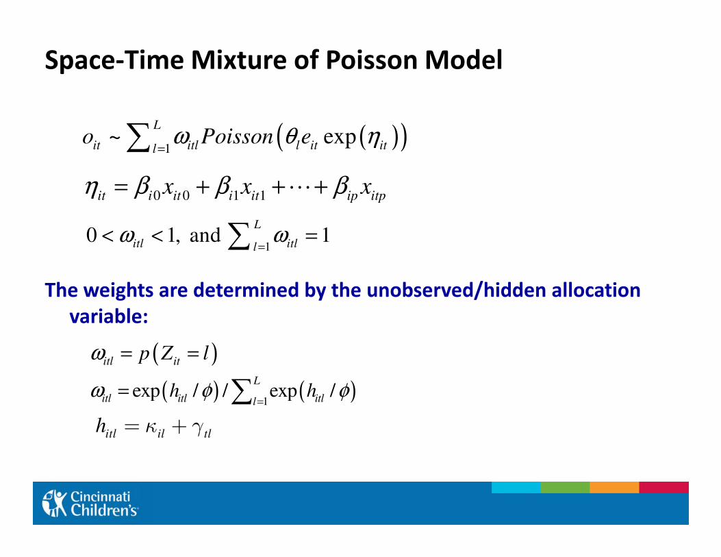
Space-Time Mixture of Poisson Model
The weights are determined by the unobserved/hidden allocation
( )( )1
~ expL
it itl l it itlo Poisson eω θ η
=∑
0 0 1 1it i it i it ip itpx x xη β β β= + + +�
10 1, and 1
L
itl itllω ω
=< < =∑
The weights are determined by the unobserved/hidden allocation
variable:
( )itl itp Z lω = =
( ) ( )1
exp / / exp /L
itl itl itllh hω φ φ
== ∑
itl il tlh κ γ= +
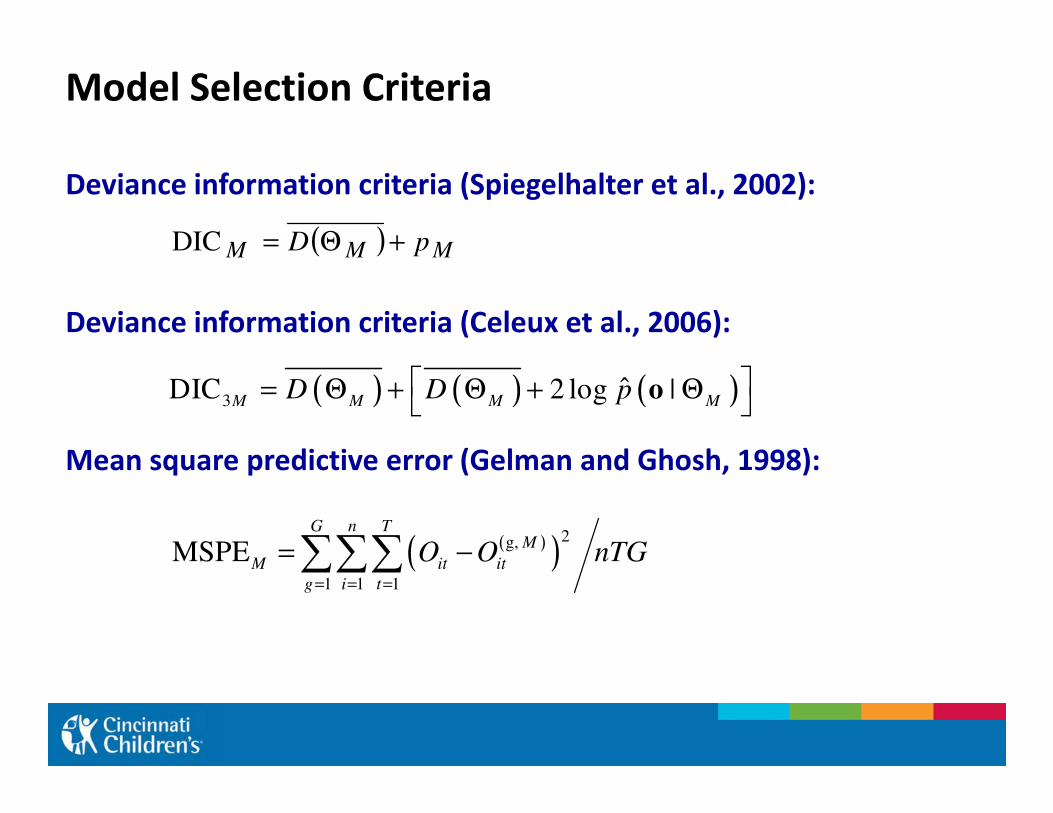
Model Selection Criteria
Deviance information criteria (Spiegelhalter et al., 2002):
Deviance information criteria (Celeux et al., 2006):
( ) MMM pD +Θ=DIC
( ) ( ) ( )3ˆDIC 2 log |
M M M MD D p = Θ + Θ + Θ
o
Mean square predictive error (Gelman and Ghosh, 1998):
( ) ( ) ( )3M M M M
( )( )2g,
1 1 1
MSPEG n T
M
M it it
g i t
O O nTG= = =
= −∑∑∑
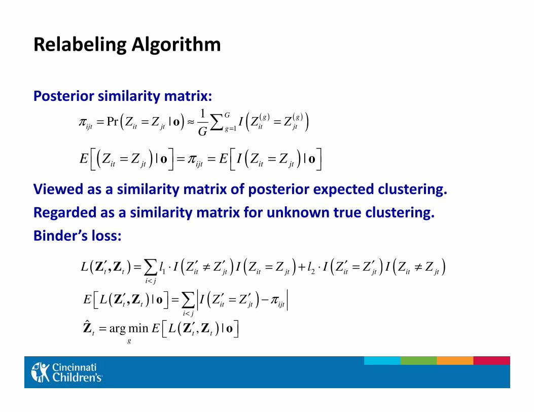
Relabeling Algorithm
Posterior similarity matrix:
Viewed as a similarity matrix of posterior expected clustering.
Regarded as a similarity matrix for unknown true clustering.
( ) ( ) ( )( )1
1Pr |
G g g
ijt it jt it jtgZ Z I Z Z
Gπ
== = ≈ =∑o
( ) ( )| |it jt ijt it jtE Z Z E I Z Zπ = = = = ο ο
Regarded as a similarity matrix for unknown true clustering.
Binder’s loss:
( ) ( ) ( ) ( ) ( )1 2t t it jt it jt it jt it jt
i j
L l I Z Z I Z Z l I Z Z I Z Z<
′ ′ ′ ′ ′= ⋅ ≠ = + ⋅ = ≠∑Z , Z
( ) ( )|t t it jt ijt
i j
E L I Z Z π<
′ ′ ′= = − ∑Z ,Z ο
( )ˆ arg min , |t t tg
E L ′= Z Z Z o
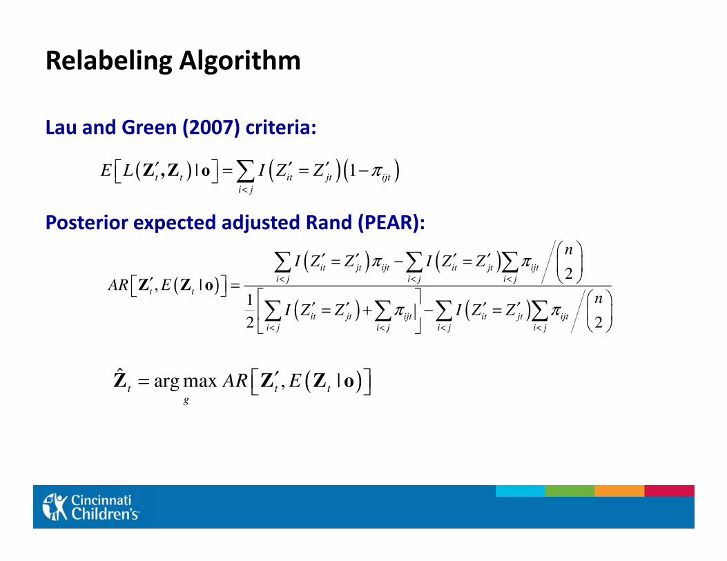
Relabeling Algorithm
Lau and Green (2007) criteria:
Posterior expected adjusted Rand (PEAR):
( ) ( )( )| 1t t it jt ijt
i j
E L I Z Z π<
′ ′ ′= = − ∑Z , Z ο
( )( ) ( )
2, |
it jt ijt it jt ijt
i j i j i j
nI Z Z I Z Z
AR E
π π< < <
′ ′ ′ ′= − =
′ =
∑ ∑ ∑Z Z o( )
( ) ( )
2, |
1
2 2
i j i j i j
t t
it jt ijt it jt ijt
i j i j i j i j
AR En
I Z Z I Z Zπ π
< < <
< < < <
′ = ′ ′ ′ ′= + − =
∑ ∑ ∑ ∑
Z Z o
( )ˆ arg max , |t t tg
AR E′= Z Z Z o
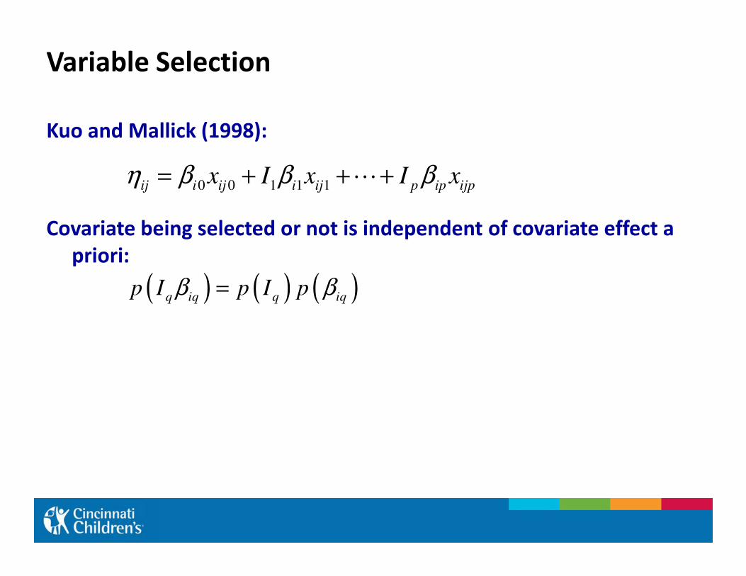
Variable Selection
Kuo and Mallick (1998):
Covariate being selected or not is independent of covariate effect a
priori:
0 0 1 1 1ij i ij i ij p ip ijpx I x I xη β β β= + + +�
( ) ( ) ( )p I p I pβ β=( ) ( ) ( )q iq q iqp I p I pβ β=
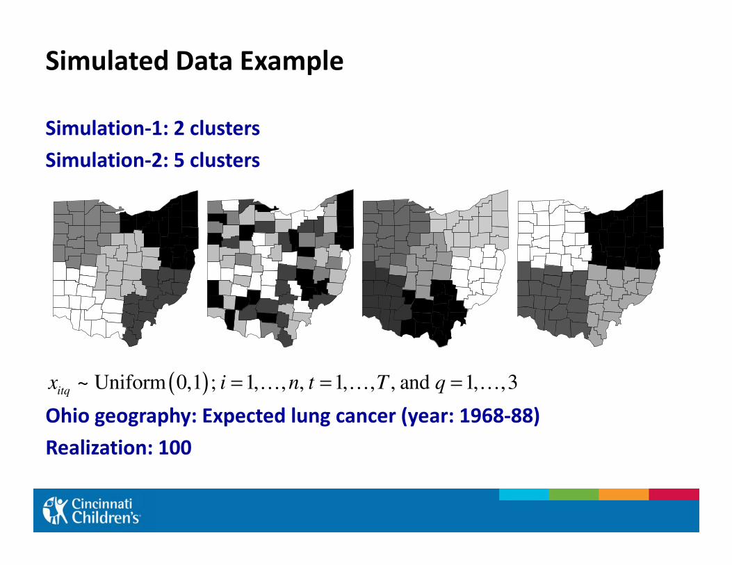
Simulated Data Example
Simulation-1: 2 clusters
Simulation-2: 5 clusters
Ohio geography: Expected lung cancer (year: 1968-88)
Realization: 100
( )~ Uniform 0,1 ; 1, , , 1, , , and 1, ,3itqx i n t T q= = =… … …
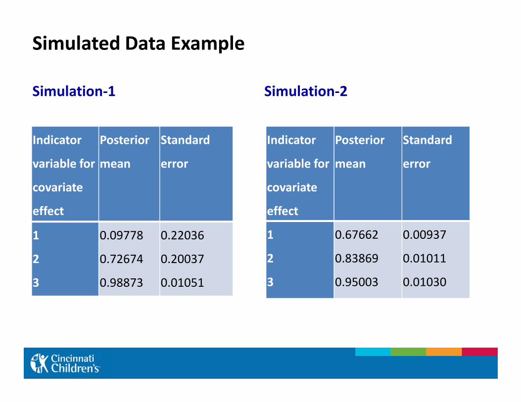
Simulated Data Example
Simulation-1 Simulation-2
Indicator
variable for
covariate
Posterior
mean
Standard
error
Indicator
variable for
covariate
Posterior
mean
Standard
error
effect
1
2
3
0.09778
0.72674
0.98873
0.22036
0.20037
0.01051
effect
1
2
3
0.67662
0.83869
0.95003
0.00937
0.01011
0.01030
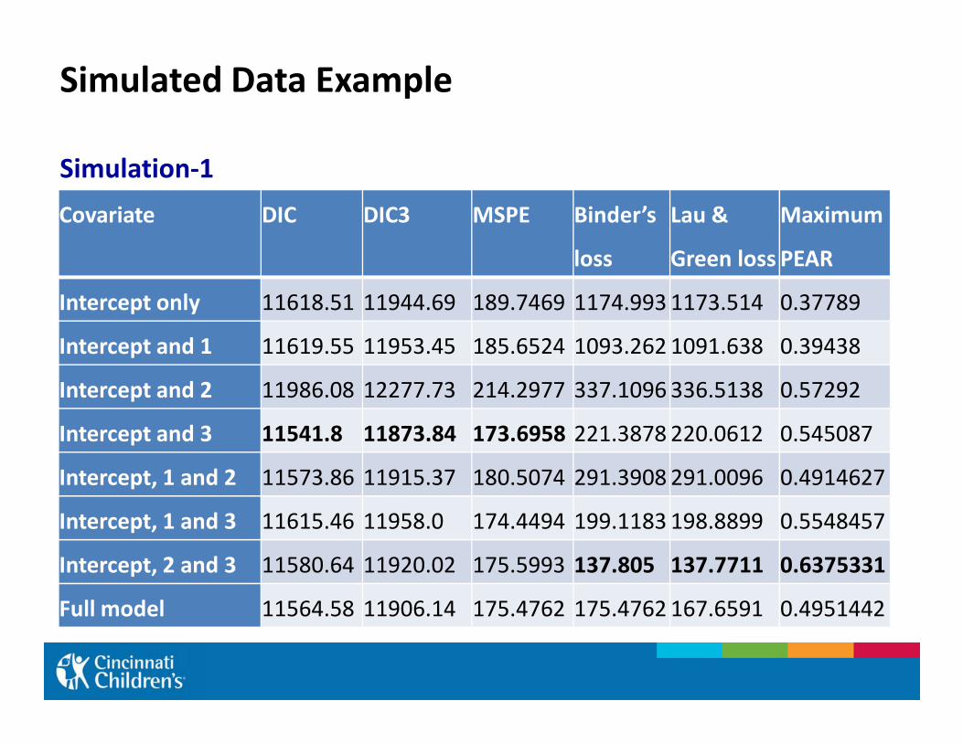
Simulated Data Example
Simulation-1
Covariate DIC DIC3 MSPE Binder’s
loss
Lau &
Green loss
Maximum
PEAR
Intercept only 11618.51 11944.69 189.7469 1174.993 1173.514 0.37789
Intercept and 1 11619.55 11953.45 185.6524 1093.262 1091.638 0.39438
Intercept and 2 11986.08 12277.73 214.2977 337.1096 336.5138 0.57292
Intercept and 3 11541.8 11873.84 173.6958 221.3878 220.0612 0.545087
Intercept, 1 and 2 11573.86 11915.37 180.5074 291.3908 291.0096 0.4914627
Intercept, 1 and 3 11615.46 11958.0 174.4494 199.1183 198.8899 0.5548457
Intercept, 2 and 3 11580.64 11920.02 175.5993 137.805 137.7711 0.6375331
Full model 11564.58 11906.14 175.4762 175.4762 167.6591 0.4951442
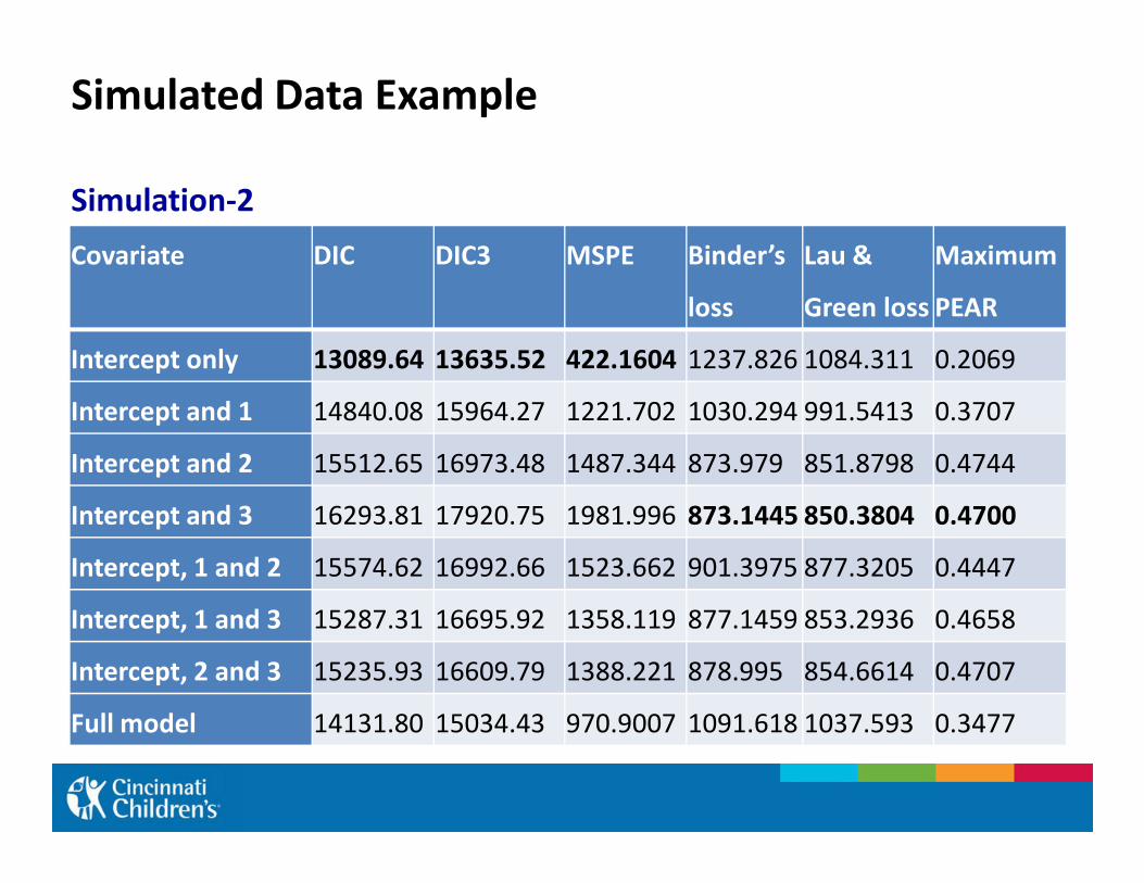
Simulated Data Example
Simulation-2
Covariate DIC DIC3 MSPE Binder’s
loss
Lau &
Green loss
Maximum
PEAR
Intercept only 13089.64 13635.52 422.1604 1237.826 1084.311 0.2069
Intercept and 1 14840.08 15964.27 1221.702 1030.294 991.5413 0.3707
Intercept and 2 15512.65 16973.48 1487.344 873.979 851.8798 0.4744
Intercept and 3 16293.81 17920.75 1981.996 873.1445 850.3804 0.4700
Intercept, 1 and 2 15574.62 16992.66 1523.662 901.3975 877.3205 0.4447
Intercept, 1 and 3 15287.31 16695.92 1358.119 877.1459 853.2936 0.4658
Intercept, 2 and 3 15235.93 16609.79 1388.221 878.995 854.6614 0.4707
Full model 14131.80 15034.43 970.9007 1091.618 1037.593 0.3477
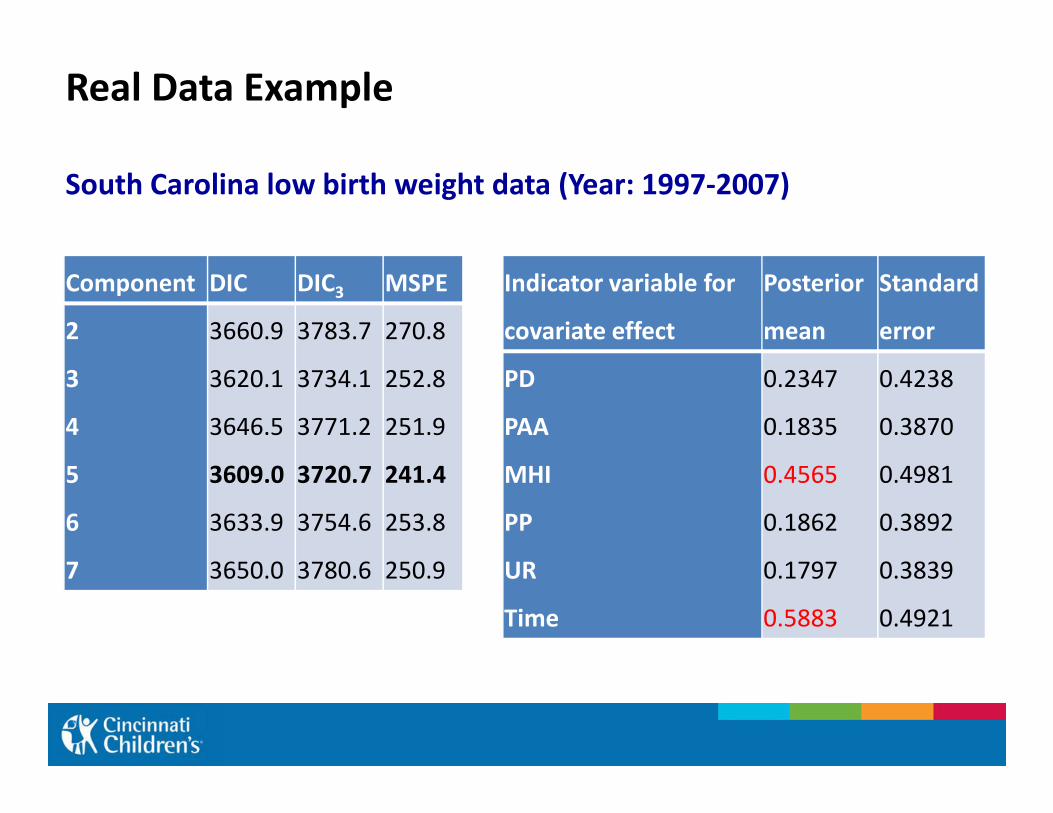
Real Data Example
South Carolina low birth weight data (Year: 1997-2007)
Component DIC DIC3 MSPE
2
3
3660.9
3620.1
3783.7
3734.1
270.8
252.8
Indicator variable for
covariate effect
Posterior
mean
Standard
error
PD 0.2347 0.4238
4
5
6
7
3646.5
3609.0
3633.9
3650.0
3771.2
3720.7
3754.6
3780.6
251.9
241.4
253.8
250.9
PAA
MHI
PP
UR
Time
0.1835
0.4565
0.1862
0.1797
0.5883
0.3870
0.4981
0.3892
0.3839
0.4921
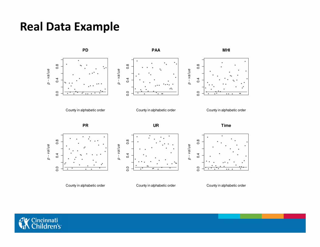
Real Data Example
**
*
*
*
*
*
**
*
*
**
*
*
*
*
**
**
*
*
*
*
*
*
*
*
*
*
*
*
*
*
*
*
*
**
*
*
**
*
*
0.0
0.4
0.8
PD
County in alphabetic order
p−
va
lue
*
*
*
*
*
*
**
*
*
*
**
*
*
*
*
*
*
*
*
*
*
*
*
*
*
**
**
*
*
*
*
******
*
*
*
*
*
0.0
0.4
0.8
PAA
County in alphabetic order
p−
va
lue
**
*
*
*
*
*
*
*
*
***
*
*
*
*
**
*
*
*
*
*
*
*
***
*
**
*
*
*
*
*
**
*
***
*
*
*
0.0
0.4
0.8
MHI
County in alphabetic order
p−
va
lue
PR UR Time
**
*
*
*
*
*
*
*
*
***
*
*
*
*
***
*
**
*
*
*
***
*
*
*
*
*
*
*
*
*
*
*
**
*
*
**
0.0
0.4
0.8
PR
County in alphabetic order
p−
va
lue
*
*
*
*
*
*
*
*
*
*
*
*
*
**
**
*
*
**
*
*
*
*
*
*
**
*
*
*
*
*
*
*
*
*
*
*
*
**
***
0.0
0.4
0.8
UR
County in alphabetic order
p−
va
lue
*
*
*
*
*
*
**
*
*
***
*
*
*
*
*
*
***
*
*
*
*
*
*
*
*
*
*
*
*
*
*
*
****
*
*
*
*
*
0.0
0.4
0.8
Time
County in alphabetic orderp
−v
alu
e
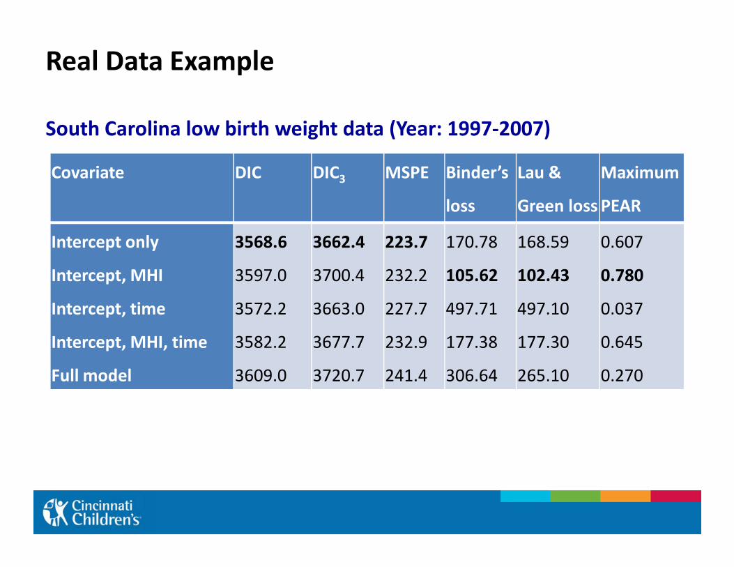
Real Data Example
South Carolina low birth weight data (Year: 1997-2007)
Covariate DIC DIC3 MSPE Binder’s
loss
Lau &
Green loss
Maximum
PEAR
Intercept only
Intercept, MHI
3568.6
3597.0
3662.4
3700.4
223.7
232.2
170.78
105.62
168.59
102.43
0.607
0.780Intercept, MHI
Intercept, time
Intercept, MHI, time
Full model
3597.0
3572.2
3582.2
3609.0
3700.4
3663.0
3677.7
3720.7
232.2
227.7
232.9
241.4
105.62
497.71
177.38
306.64
102.43
497.10
177.30
265.10
0.780
0.037
0.645
0.270
Conclusions
Previously, Best et al. (2005) showed that the spatial model with
convolution prior (e.g. Besag et al., 1991) overestimate the risk
surface for the high risk areas and the best model selected by the
DIC is not always able to select the right clusters.
We used a space-time mixture of Poisson regression model with
homogeneous covariate effects.
We designed two simulation studies with smaller and larger numbers
of clusters, and with common covariate effects. The covariates are
generated with stronger to weak levels of spatial correlation.
In our simulated and real datasets, we observed that model selection
criteria do not indicate to the right cluster model.
Conclusions
Limitations:
Simultaneous estimation of the number of clusters and variable
selection for spatial data
Improvement the DIC performance:
Variational Bayes approach (McGrory and Titterington, 2007)Variational Bayes approach (McGrory and Titterington, 2007)
Viewing DIC as an approximate penalized loss function (Plummer,
2008)
Model based relabeling algorithm where the label for each
observation is chosen by maximizing the classification probability
(Yao, 2012)
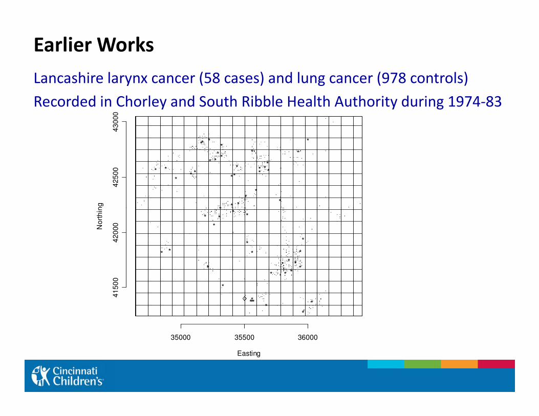
Earlier Works
Lancashire larynx cancer (58 cases) and lung cancer (978 controls)
Recorded in Chorley and South Ribble Health Authority during 1974-83
*
*
*
*
***
*
*
*
*
*
**
*
*
*
*
**
**
* *
*
**
*
*
*
42
500
43
00
0
Nort
hin
g
*
*
**
*
*
*
*
**
*
*
*
*
*
** **
*
*
**
*
*
*
*****
35000 35500 36000
41
50
04
20
00
Easting
Nort
hin
g
Earlier Works
Point process modeling (CSDA, 2010):
Approximate likelihood
Berman-Turner (BT) model
Conditional logistic (CL) model
Binomial mesh (BM) model
Poisson mesh (PM) modelPoisson mesh (PM) model
Earlier Works
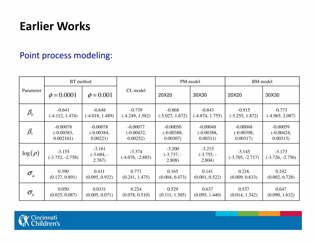
Point process modeling:
Parameter
BT method
CL model
PM model BM model
20X20 30X30 20X20 30X30
-0.641
(-4.112, 1.474)
-0.648
(-4.018, 1.489)
-0.739
(-4.249, 1.582)
-0.868
(-5.027, 1.672)
-0.843
(-4.874, 1.755)
-0.915
(-5.255, 1.872)
-0.773
(-4.965, 2.087)0β
0.0001φ = 0.001φ =
-0.00078
(-0.00383,
0.002161)
-0.00078
(-0.00384,
0.00221)
-0.00077
(-0.00432,
0.00252)
-0.00050
(-0.00388,
0.00307)
-0.00048
(-0.00388,
0.00311)
-0.00048
(-0.00398,
0.00317)
-0.00059
(-0.00424,
0.00313)
-3.155
(-3.752, -2.758)
-3.161
(-3.684, -
2.767)
-3.374
(-4.076, -2.885)
-3.200
(-3.737, -
2.808)
-3.215
(-3.755, -
2.804)
-3.145
(-3.705, -2.717)
-3.173
(-3.726, -2.756)
0.390
(0.127, 0.891)
0.411
(0.095, 0.932)
0.771
(0.241, 1.475)
0.165
(0.004, 0.473)
0.141
(0.001, 0.522)
0.216
(0.009, 0.633)
0.242
(0.002, 0.728)
0.050
(0.025, 0.087)
0.0331
(0.005, 0.071)
0.224
(0.078, 0.510)
0.529
(0.111, 1.305)
0.637
(0.095, 1.440)
0.537
(0.014, 1.342)
0.647
(0.090, 1.632)
1β
( )log ρ
uσ
νσ
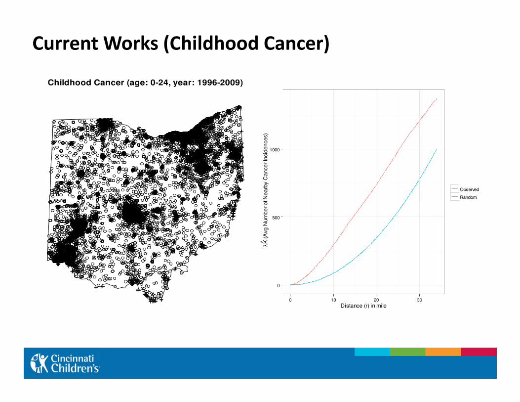
Current Works (Childhood Cancer)
Childhood Cancer (age: 0-24, year: 1996-2009)
+
+
++++++++++ +
+
+
+
+++
+
++++
+++++
+++
++
++
++ 1000
(A
vg N
um
ber of N
earb
y C
ancer In
cid
ences)
Observed
Random
+++
++++++++
++
++++++++
++
+++
++++++
+++ ++
++
+++
++ +++ ++
+ +++++++
+++
++
++
++++
+++
+++
++
++
+++++
+++++
+++
+++
++++
0
500
0 10 20 30
Distance (r) in mile
λK^
(A
vg N
um
ber of N
earb
y C
ancer In
cid
ences)
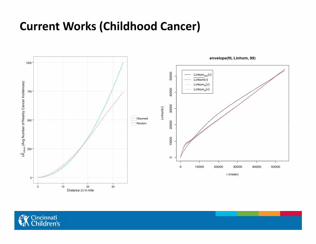
Current Works (Childhood Cancer)
500
750
1000
(A
vg
Nu
mb
er
of N
ea
rby C
an
ce
r In
cid
en
ce
s)
Observed
Random
20000
30000
40000
50000
envelope(fit, Linhom, 99)
Lin
hom
(r)
Linhomobs(r)
Linhom(r)
Linhomhi(r)
Linhomlo(r)
0
250
0 10 20 30
Distance (r) in mile
λK^
inh
om (
Avg
Nu
mb
er
of N
ea
rby C
an
ce
r In
cid
en
ce
s)
Random
0 10000 20000 30000 40000 50000
010000
20000
r (meter)

Thanks!