Space-scale-time dynamics of liquid–gas shear flow

HAL Id: hal-03142246https://hal.archives-ouvertes.fr/hal-03142246

Submitted on 15 Feb 2021

HAL is a multi-disciplinary open accessarchive for the deposit and dissemination of sci-entific research documents, whether they are pub-lished or not. The documents may come fromteaching and research institutions in France orabroad, or from public or private research centers.

L’archive ouverte pluridisciplinaire HAL, estdestinée au dépôt et à la diffusion de documentsscientifiques de niveau recherche, publiés ou non,émanant des établissements d’enseignement et derecherche français ou étrangers, des laboratoirespublics ou privés.

Space-scale-time dynamics of liquid–gas shear flowF. Thiesset, T. Ménard, C. Dumouchel

To cite this version:F. Thiesset, T. Ménard, C. Dumouchel. Space-scale-time dynamics of liquid–gas shear flow. Journalof Fluid Mechanics, Cambridge University Press (CUP), 2021, 912, 10.1017/jfm.2020.1152. hal-03142246

https://hal.archives-ouvertes.fr/hal-03142246

https://hal.archives-ouvertes.fr

This draft was prepared using the LaTeX style file belonging to the Journal of Fluid Mechanics 1

Space-scale-time dynamics of liquid-gasshear flow

F. Thiesset1:, T. Menard1, C. Dumouchel1

1CNRS, Normandy Univ., UNIROUEN, INSA Rouen, CORIA, 76000 Rouen, France

(Received xx; revised xx; accepted xx)

Two-point statistical equations of the liquid phase indicator function are used to appraisethe physics of liquid-gas shear flows. The contribution of the different processes in thecombined scale/physical space is quantified by means of direct numerical simulations ofa temporally liquid-gas shear layer. Light is first shed onto the relationship between two-point statistics of the phase indicator and the geometrical properties of the liquid/gasinterface, namely its surface density, mean and Gaussian curvatures. Then, the theoryis shown to be adequate for highlighting the preferential direction of liquid transportin either scale or flow positions space. A direct cascade process, i.e. from large tosmall scales, is observed for the total phase indicator field, while the opposite appliesfor the randomly fluctuating part suggesting a transfer of ’energy’ from the mean tothe fluctuating component. In the space of positions within the flow, the flux tend toredistribute energy from the centreline to the edge of the shear layer. The influence ofthe mean shear rate and statistical inhomogeneities on the different scales of the liquidfield are revealed.

Key words:

1. Introduction

Two-phase flows, e.g. liquid/gas flows, or more generally flows involving two immisciblephases are widely encountered in natural, domestic or industrial situations. At sufficientlyhigh injection velocity, such flows have strong propensity to break up into a myriad ofliquid fragments, subsequently atomizing into a stream of dispersed droplets in a gaseousatmosphere, called spray. The process of successive disintegration of a bulk liquid flowinto a stream of drops is referred to as liquid atomization.Liquid atomization is essentially a multi-scale and multi-dimensional phenomenon,

i.e. with dynamics that are generally turbulent, which can differ significantly dependingon the region of the flow, the sizes of the involved liquid structures and the fluid/flowphysical parameters. Before breaking-up into spherical droplets, these liquid structureshave complex geometry, morphology and topology whose description still remains a chal-lenging task (Di Battista et al. 2019; Essadki et al. 2019; Thiesset et al. 2019b). Anotherdifficulty resides in the local and singular nature of liquid break-up. Indeed, atomizationresults from topological transitions due to local pinch-off of liquid necks, a nice physicalexample of the formation of singularities at finite time (e.g. Eggers & Villermaux 2008,and references therein). Exploring and predicting liquid atomization thus necessitatessome sophisticated theoretical tools, among which some need yet to be elaborated. When

: Email address for correspondence: [email protected]

2 F. Thiesset, T. Menard, C. Dumouchel

compared to single phase flows, the complexity in the theoretical description of two-phaseflows rises in a significant manner. Indeed, the presence of the liquid-gas interface andhence surface tension effects, together with the density and viscosity jump across theinterface make inoperative most of available theoretical results obtained in the contextof single phase turbulence (Gorokhovski & Herrmann 2008). Some specific theories arethus required.However, although the presence of such an interface could appear as an overwhelming

obstacle, it also constitutes a glaring anchor point. One can indeed conjecture that manykey facets of the multi-scale and multi-dimensional character of the whole flow can bequantified solely through the multi-scale and multi-dimensional characteristics of theliquid-gas interface. Similarly, instead of characterizing the scale/space/time propertiesof the whole turbulent velocity field, one can focus on the scale/space/time properties ofthe transport of liquid relative to the gas phase, thereby reducing the analysis to a singlescalar field variable, viz. the liquid phase indicator field. Further, as will be thoroughlydetailed later, by use of a statistical analysis, the singular nature of liquid break-up islikely to be smoothed out by the averaging procedures. It is then expected that onceaveraged, liquid atomization (i) recovers some degree of regularity so that the dynamicsof liquid structures appear continuous, (ii) retrieves some degree of predictability in thestatistical sense. These are the key hypotheses the present paper aims at discussing.Here, the multi-scale features of liquid/gas turbulent flows is appraised using the recent

theoretical framework proposed by Thiesset et al. (2020). This theory is inspired bythe generalized Karman-Howarth-Kolmogorov equation (e.g. Danaila et al. 2004; Hill2002; Portela et al. 2017; Casciola et al. 2003; Marati et al. 2004, and reference therein)which is adapted to a relevant scalar of two-phase flows: the phase indicator function.As shown by Thiesset et al. (2020), this new framework is promising for characterizingturbulent liquid/gas flows because, (i) the notion of scale is explicit and unambiguouslydefined, (ii) it is exact and thus applies to the entire flow field, from the injectionto the spray dispersion zone and irrespective of the flow configuration or regime, (iii)the effect of different physical parameters (surface tension, viscosity and density, inflowvelocity conditions), although implicit in the equations, can be probed as a function ofthe scale and flow position. Thiesset et al. (2020) reported an analysis of a statisticallyhomogeneous flow evolving in a triply periodic box which was numerically simulated usingthe code ARCHER. This particular configuration is not influenced by any preferentialforcing direction. Hence, the liquid-phase statistics were invariant by translation withinthe flow thereby reducing the problem to a scale/time analysis only. Here, we aim atextending the study of Thiesset et al. (2020), by exploring the full scale/space/timeevolution of the liquid phase in a flow which reveals a substantial degree of inhomogeneity:a liquid/gas shear layer. This is a new test case for the proposed formalism using two-point statistics. This flow configuration is one step further towards real atomizationsituation since the forcing effect due to a mean velocity gradient is included. Althoughstill quite far from a real situation, it is archetypal of the so-called air-assisted atom-ization (Lasheras & Hopfinger 2000; Marmottant & Villermaux 2004; Fuster et al. 2013;Ling et al. 2017, 2019).Additionally, because two-phase flows are not the only physical situations where a

discontinuity separates two media of different natures, our objective is to address thisquestion within the broader context of heterogeneous media. Therefore, we expect someof our elaborations to apply not only to two-phase flows but we hope that they can helpbetter characterizing the structure and dynamics of heterogeneous fields in general suchas for instance porous media, fractal aggregates or colloids.The paper is organized as follows. First, the theoretical framework firstly reported

Space-scale-time dynamics of liquid-gas shear flow 3

x`

x´

X

r

2

´ r

2

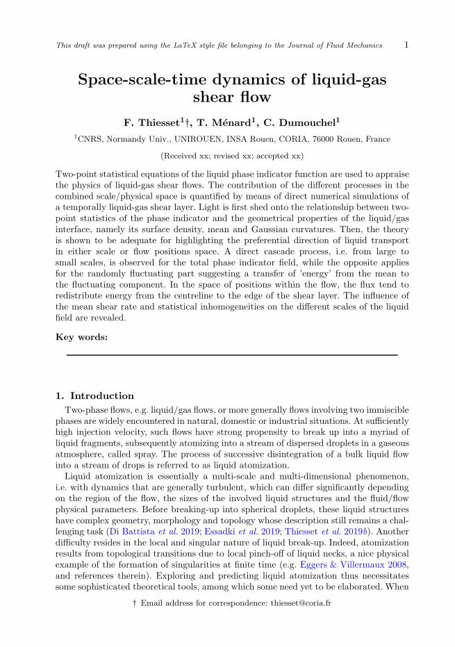
Figure 1: Schematic representation of two points x` and x´, the midpoint X “ pX,Y, Zqand the separation vector r “ prx, ry, rzq.

by Thiesset et al. (2020) is recalled briefly in section §2. Section §3 is devoted to thepresentation of the two-phase flow solver ARCHER which was used to simulate theliquid-gas shear layer under consideration. The numerical database used to appraisethe contribution of the different terms of the equations is detailed. A third section §4aims at emphasizing the close relationship between two-point statistics of the liquidphase indicator function and some geometrical properties of the liquid/gas interface andliquid structures. The space/scale/time evolution of the liquid phase in the shear layer isperformed for both the total and the fluctuating field in section §5 and §6, respectively.The paper closes with some conclusions.

2. Space-scale-time analysis of liquid transport

The present study follows the lines of Thiesset et al. (2019a, 2020) and is based on ananalysis of the phase indicator field φ which is 1 (or 0) in the liquid (or gas) phase. Asper Thiesset et al. (2019a, 2020), we define the second order structure functions of φ, asthe averaged squared difference of φ between two arbitrary points separated by a vectorr (see Fig. 1) viz.

@

pδφq2D

E“

A

“

φpx`q ´ φpx´q‰2

E

E

“

B

”

φ´

X `r

2

¯

´ φ´

X ´r

2

¯ı2F

E

(2.1)

where the brackets denote average and the subscript E indicates an ensemble average.As seen in Fig. 1, the mid-point is defined by X “ px` ` x´q2 and the separationvector r “ px` ´ x´q (Hill 2002). A physical interpretation of pδφq2 is provided later in§4. Because we consider the averaged squared difference of φ, we sometimes refer pδφq2

to as the ’energy’ content at a given scale, in analogy with the second-order structurefunction of the velocity field which effectively represents a kinetic energy at a given scale.Alternatively, we call pδφq2 the scale-distribution.

Thiesset et al. (2019a, 2020) derived the transport equation for the second orderstructure functions of the phase indicator field. They considered the equation not only


for the total field φ but also fluctuating field φ1 “ φ ´ xφyE, viz.

Bt

A

pδφq2E

E

“ ´∇r‚

A

pδuq pδφq2E

E

´ ∇X‚

A

pσuq pδφq2E

E

(2.2a)

Bt

A

`

δφ1˘2

E

E

“ ´∇r‚

A

pδuq`

δφ1˘2

E

E

´ 2@

pδφ1qpδu1qD

E‚ ∇r xδφy

E

´∇X‚

A

pσuq`

δφ1˘2

E

E

´ 2@

pδφ1qpσu1qD

E‚ ∇X xδφy

E(2.2b)

Bt denote the time derivative. ∇r and ∇X are the gradient operators in the r and X

space, respectively. δ‚ and σ‚ represent the difference and the average of a given quantitybetween the two-points considered. At this level, the different terms of Eqs. (2.2a) and(2.2b) depend on X ” pX,Y, Zq (the mid-point between the two-points correspondingto the position within the flow), r ” prx, ry, rzq (the separation vector whose magnitudecan be associated to the probed scale) and time t, i.e. a 7 dimensional problem. Themethodology for deriving these equations is described in great details by Thiesset et al.(2020); Hill (2002); Danaila et al. (2004) and is not recall here. It is only worth notingthat Eqs. (2.2a) and (2.2b) are exact equations which can be derived directly from thetransport equation for the phase indicator supposing the flow incompressible with nophase change. Eqs. (2.2a) and (2.2b) explicitly account for the anisotropic (through thedependence to the separation vector r) and inhomogeneous (through the appearance ofthe position space X) characters of the flow.

2.1. Average along homogeneity directions

Here, we explore the specific configuration of a temporally evolving shear layer with twohomogeneity directions in the streamwize x and spanwize directions z (see §3). Therefore,planar averages over the set of points PpY q “ tX,Y, Z | Y, 0 ď X ď Lx, 0 ď Z ď Lzucan be used in place of ensemble averages. Lx and Lz represent the size of the averagingdomain in the streamwize and spanwize directions, respectively. Eqs. (2.2a) and (2.2b)then reduce to

Bt

A

pδφq2E

Ploooooomoooooon

dt term

“ ´∇r‚

A

pδuq pδφq2E

Ploooooooooooomoooooooooooon

r´Transfer

´BY

A

pσv1q pδφq2E

Plooooooooooomooooooooooon

Y ´Transfer

(2.3a)

Bt

A

`

δφ1˘2

E

Ploooooomoooooon

dt term

“ ´∇r‚

A

pδuq`

δφ1˘2

E

Plooooooooooooomooooooooooooon

r´Transfer

´2@

pδφ1qpδv1qD

PBry xδφy

Ploooooooooooooooomoooooooooooooooon

r´Production

´BY

A

`

σv1˘ `

δφ1˘2

E

Ploooooooooooomoooooooooooon

Y ´Transfer

´2@

pδφ1qpσv1qD

PBY xδφy

Ploooooooooooooooomoooooooooooooooon

Y ´Production

(2.3b)

where we have used xvyP “ 0 and hence v “ v1. Eq. (2.3a) is the transport equation forthe second-order structure function of the total field φ. It reveals that time variationsof xpδφq2yP are due to the combined effect of two transfer processes (more preciselydivergence of fluxes) which occur concomitantly in scale r and physical space Y . Thetransfer in scale space, abbreviated by the r-transfer term quantifies the direction andamplitude of the cascade process, i.e. the transfer of the quantity xpδφq2yP betweendifferent orientations and modulus of the vector r. Hereafter in this paper, the word’cascade’ will be used to designate the transfer of ’energy’ between scales which ismathematically given by the r-divergence term in Eqs. (2.3a) and (2.3b). The othertransfer term, abbreviated Y -transfer represents the transport of a given liquid scale ingeometrical space, i.e. from one position within the flow (here one Y plane location) toanother.


Eq. (2.3b) pertains to the fluctuating component φ1. In addition to similar transferterms, the latter contains two additional processes, namely two production processeswhich again act concomitantly in scale and physical space. The production process isassociated with the presence of inhomogeneities, i.e. some gradients of liquid volumefraction xφyP. As was proved by Thiesset et al. (2020), this production mechanism canalso be interpreted as an exchange of liquid between the mean and the fluctuatingfields which acts in homogenizing the mean volume fraction field. Further physicalinterpretations and algebraic decompositions of the different terms of Eqs. (2.3a) and(2.3b) are provided by Thiesset et al. (2020) but are not considered in the present study.Note here again that Eqs. (2.3a) and (2.3b) hold even if the flow is anisotropic and

inhomogeneous.

2.2. Average over all directions of the separation vector

The different terms of Eqs. (2.3a) and (2.3b) have argument list (r, Y, tq, i.e. a 5Dproblem. The dependence of statistics to the separation vector r embeds the anisotropiccharacter of the transport of liquid which is of major importance in this flow. However,substantial information can first be gained by averaging over all orientations of theseparation vector r, thereby reducing the problem complexity to a 3D problem withargument list (|r|, Y, tq. This can be achieved in two fashions. The first method is toperform an angular average over all solid angles. This operation is noted x‚yΩ and isdefined by

x‚yΩ “1

4π

ĳ

Ω

‚ sin θdθdϕ (2.4)

where the set of solid angles Ω “ tϕ, θ | 0 ď ϕ ď π, 0 ď θ ď 2πu with ϕ “ arctanpryrxqand θ “ arccosprz|r|q. The angular average is related to the spherical average within asphere of radius r “ |r|, noted x‚yS and defined by (Thiesset et al. 2020; Hill 2002):

x‚yS “3

4πr3

¡

S

‚ r2 sin θdθdϕdr “3

r3

ż r

0

x‚yΩ r2dr (2.5)

2.3. Average along the inhomogeneity direction

Finally, a spatial average can further be performed. In our case, the latter operates onthe Y direction and writes

x‚yY “2

Ly

ż

Y

‚ dY (2.6)

with Y “ tY | ´ Ly4 ď Y ď Ly4u (Y “ 0 is located at the shear layer centreline).Using the gradient theorem, averaging over Y allows us simplifying the Y -Transfer termsas follows

A

BY

A

`

σv1˘

pδφq2E

P

E

Y

“A

`

σv1˘

pδφq2E

PpY “Ly

4q

Á

`

σv1˘

pδφq2E

PpY “´Ly

4q(2.7a)

A

BY

A

`

σv1˘ `

δφ1˘2

E

P

E

Y

“A

`

σv1˘ `

δφ1˘2

E

PpY “Ly

4q

Á

`

σv1˘ `

δφ1˘2

E

PpY “´Ly

4q(2.7b)

2.4. Summary

In summary, roughly speaking, an angular (spatial) average enables studying thetime/scale/space transport of liquid structures independently of their orientations (posi-tion in the flow). Consequently, these different averaging procedures have the advantage


of reducing the problem complexity but is automatically accompanied by a loss ofinformations which can be summarized as follows.

‚ x‚yP leads to a problem in 5D, with argument list pr, Y, tq. It corresponds to themore general version of the equations in the temporally evolving shear layer with x andz being homogeneity directions.

‚ x‚yP,Ω yields a problem in 3D, with argument list pr, Y, tq, the information about thepreferential orientation (anisotropy) of the liquid structures is lost.

‚ x‚yP,Ω,Y corresponds to a 2D problem, with argument list pr, tq, the informationabout the locality within the flow is lost.In the present paper, for the sake of pedagogy, we start by considering the most

simplified version of the problem (angularly and spatially averaged budgets) and thensuccessively lift some averaging operations up to the more general version of the two-point transport equations. Most of the present analysis is rendered feasible thanks todata from numerical simulations. In the following sections, we describe the simulationcode and database.

3. Numerical simulations of liquid-gas shear flow

3.1. The ARCHER code

The liquid-gas shear flow is simulated using the High-Performance-Computing codeARCHER developed at the CORIA laboratory (Menard et al. 2007). It is based on theone-fluid formulation of the incompressible Navier-Stokes equation which is solved on aCartesian mesh, viz.

Bt ρu ` ∇ ‚ pρu b uq “ ´∇p ` ∇ ‚ p2µDq ` f ` γHδsn. (3.1)

p is the pressure field, D the strain rate tensor, f a source term, µ the kinematicviscosity, ρ the density, γ the surface tension, n the unit normal vector to the liquid-gasinterface, H its mean curvature and δs is the Dirac function characterizing the locationof the liquid gas interface. For solving Eq. (3.1), the convective term is written inconservative form and solved using the improved Rudman (1998) technique presentedin Vaudor et al. (2017). The Sussman et al. (2007) method is used to compute theviscous term. To ensure incompressibility of the velocity field, a Poisson equation issolved. The latter accounts for the surface tension force and is solved using a MultiGridpreconditioned Conjugate Gradient algorithm (MGCG) (Zhang 1996) coupled with aGhost-Fluid method (Fedkiw et al. 1999).A coupled level-set and volume-of-fluid (CLSVOF) solver is used for transporting

the interface, the level-set function accurately describing the geometric features of theinterface (its normal and curvature) and the volume-of-fluid function ensuring mass con-servation. The density is calculated from the volume-of-fluid (or liquid volume fraction) asρ “ ρlφ`ρgp1´φq, where ρl, ρg is the density of the liquid and gas phase. The dynamicviscosity (µl or µg) depends on the sign of the Level Set function. In cells containingboth a liquid and gas phase, a specific treatment is performed to evaluate the dynamicviscosity, following the procedure of Sussman et al. (2007). For more information aboutthe ARCHER solver, the reader can refer to e.g. Menard et al. (2007); Duret et al. (2012);Vaudor et al. (2017).

3.2. Numerical domain and flow features

The flow configuration is that of a planar liquid layer being sheared by a gas stream.The flow is directed towards the x axis, z denotes the spanwize and y the vertical axis,


respectively. The calculation domain is Lx ˆLy ˆLz “ 8ˆ 4ˆ 4 cm3 in the streamwize,vertical and spanwize direction respectively. The liquid and gas properties correspond tothat of water and air at ambient pressure. The dynamic viscosity µ [kg.m´1.s´1] is µl =1.0 10´3 and µg = 1.8 10´5 for the liquid and gas phase, respectively. The fluid density ρ

[kg.m´3] is ρl = 1.0 103 and ρg = 1.2, respectively. The surface tension γ “ 0.072 N.m´1.Close to the liquid-gas interface, an error function profile for the streamwize velocity

u is initially prescribed and is given by

upx, y, zq “ug

2

„

1 ` erf

"

86.83

ˆ

y

Ly

´1

2

˙*

. (3.2)

The spanwize w and vertical v velocity components vpx, y, zq “ wpx, y, zq “ 0. ug “7.5m.s´1 denotes the maximum gas velocity. The constant 86.83 corresponds to a vorticitythickness of δω “ 1.15 mm. This was set so that the most unstable wavelength of theKelvin-Helmholtz instability is expected to be half of Lx and the spanwize Rayleigh-Taylor instability has a wavelength of about Lz6 (Marmottant & Villermaux 2004).These two modes were forced in the present simulation by superimposing to the liquid-gas interface a small sinusoidal perturbation with period Lx2 and Lz6 in the streamwizeand spanwize directions, respectively. This was done to trigger the destabilization of theliquid layer and consequently reduce the overall computational time. The initialized level-set function G was set as follows:

Gpx, y, zq “

ˆ

Ly

2´ y

˙

`Ly

200

„

sin

ˆ

4πx

Lx

˙

` sin

ˆ

12πz

Lz

˙

(3.3)

Periodic boundary conditions are used in the streamwize and spanwize direction. A no-slip boundary condition is applied to the bottom frontier while an outflow condition isused at the uppermost boundary of the calculation domain. The mesh size consisted ofNx ˆ Ny ˆ Nz “ 512 ˆ 256 ˆ 256 cells and 1024 processors are used. This correspondsto a cell size ∆x “ ∆y “ ∆z « 0.156 mm. The question of the adequacy of a givenresolution depends on the physical quantity of interest. Indeed, the resolution neededfor some large-scale quantities such as the turbulent kinetic energy or the liquid volumefraction to be grid independent is most likely not the same than the one needed forsome small scales quantities (e.g. the enstrophy) to be faithfully resolved. As emphasizedin subsequent sections, the budgets given by Eqs. (2.3a) and (2.3b) will be proved tobe nicely closed proving that the present resolution is adequate, at least as far as theliquid-gas interface properties are concerned.The initial Weber number based on the gas velocity ug and the shear layer vorticity

thickness δω is Weg “ ρgu2gδωγ “ 1.08. As per Taguelmimt et al. (2016), we define the

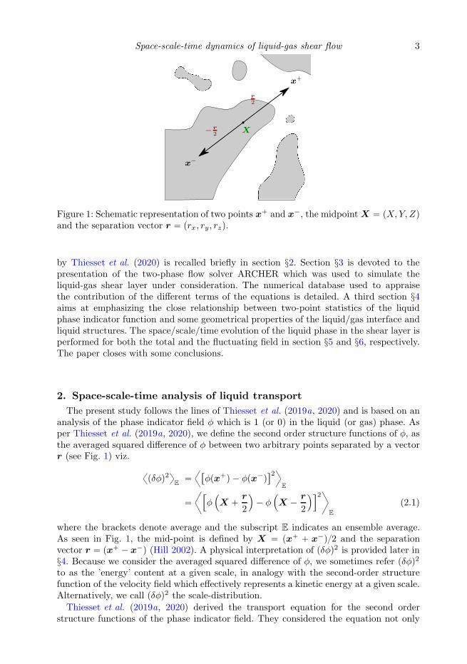
Reynolds number by use of the average dynamic viscosity , i.e. Re “ 2ugδωpνg ` νlq “1078.Typical snapshots of the flow simulation are presented in Fig. 2. The overall

phenomenology of this flow is quite similar to what is commonly referred to as anair-assisted atomization process as documented by e.g. Lasheras & Hopfinger (2000);Marmottant & Villermaux (2004); Fuster et al. (2013). The rapid destabilization of theliquid-gas interface is observed to be followed by the oblique ejection of ligaments whichsubsequently breaks into a myriad of droplets. Qualitatively, one observes that the degreeof tortuousness of the liquid gas interface is increasing from t˚ “ 0.98 up to t˚ “ 1.37 andthen becomes smoother at t˚ “ 1.83. Further, while liquid structures manifest mainlyas ligaments at t˚ “ 0.98 and t˚ “ 1.37, some detached droplets are clearly identified att˚ “ 1.83. The break-up mechanism thus occurs between t˚ “ 1.37 and t˚ “ 1.83. Stillat t˚ “ 1.83, the interface separating the liquid and gas phase located near the centreline

8 F. Thiesset, T. Menard, C. Dumouchelt˚ “ 0.98

t˚ “ 1.37

t˚ “ 1.83x

y

z

Figure 2: Typical snapshots of the simulation. The flow is from left to right. Theliquid-gas interface is initially perturbed with a sinusoidal pattern which promotes thedestabilization of the flow thereby reducing the overall computational cost. From left toright, top to bottom t˚ “ tLxug “ 0.98, 1.37, 1.83.

of the shear layer is experiencing a relaxation mechanism most likely attributed to theincreasing influence of surface tension relative to the decreasing shear rate. This flowconfiguration thus reveals some multi-scale features and a concomitant transport of theliquid phase in scale and flow position space. It is therefore a very nice candidate forbeing explored with two-point statistical equations. However, it is worth stressing thatthe present simulation, reveals much less complex physics than the one presented by e.g.


Y “ 0

Y “ Ly4

Y “ Ly2

Y “ ´Ly2

Y “ ´Ly4

maxpY q “ Ly4

maxpy`q “ maxpY q ` maxpryq2 “ Ly2

minpy´q “ minpY q `minpryq2 “ ´Ly2

minpY q “ ´Ly4

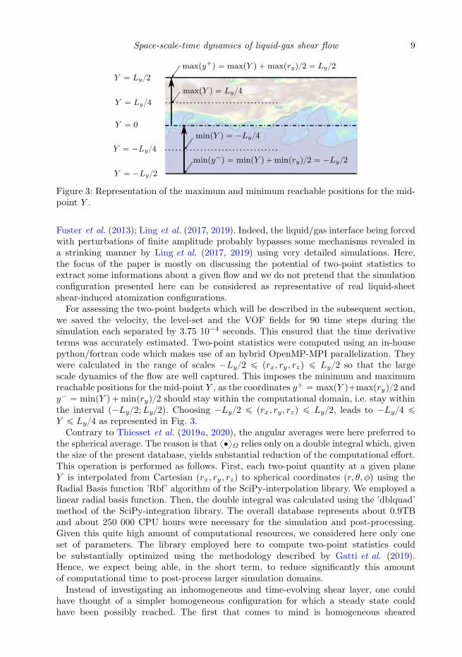
Figure 3: Representation of the maximum and minimum reachable positions for the mid-point Y .

Fuster et al. (2013); Ling et al. (2017, 2019). Indeed, the liquid/gas interface being forcedwith perturbations of finite amplitude probably bypasses some mechanisms revealed ina strinking manner by Ling et al. (2017, 2019) using very detailed simulations. Here,the focus of the paper is mostly on discussing the potential of two-point statistics toextract some informations about a given flow and we do not pretend that the simulationconfiguration presented here can be considered as representative of real liquid-sheetshear-induced atomization configurations.For assessing the two-point budgets which will be described in the subsequent section,

we saved the velocity, the level-set and the VOF fields for 90 time steps during thesimulation each separated by 3.75 10´4 seconds. This ensured that the time derivativeterms was accurately estimated. Two-point statistics were computed using an in-housepython/fortran code which makes use of an hybrid OpenMP-MPI parallelization. Theywere calculated in the range of scales ´Ly2 ď prx, ry, rzq ď Ly2 so that the largescale dynamics of the flow are well captured. This imposes the minimum and maximumreachable positions for the mid-point Y , as the coordinates y` “ maxpY q`maxpryq2 andy´ “ minpY q `minpryq2 should stay within the computational domain, i.e. stay withinthe interval p´Ly2;Ly2q. Choosing ´Ly2 ď prx, ry, rzq ď Ly2, leads to ´Ly4 ďY ď Ly4 as represented in Fig. 3.Contrary to Thiesset et al. (2019a, 2020), the angular averages were here preferred to

the spherical average. The reason is that x‚yΩ relies only on a double integral which, giventhe size of the present database, yields substantial reduction of the computational effort.This operation is performed as follows. First, each two-point quantity at a given planeY is interpolated from Cartesian prx, ry , rzq to spherical coordinates pr, θ, φq using theRadial Basis function ’Rbf’ algorithm of the SciPy-interpolation library. We employed alinear radial basis function. Then, the double integral was calculated using the ’dblquad’method of the SciPy-integration library. The overall database represents about 0.9TBand about 250 000 CPU hours were necessary for the simulation and post-processing.Given this quite high amount of computational resources, we considered here only oneset of parameters. The library employed here to compute two-point statistics couldbe substantially optimized using the methodology described by Gatti et al. (2019).Hence, we expect being able, in the short term, to reduce significantly this amountof computational time to post-process larger simulation domains.Instead of investigating an inhomogeneous and time-evolving shear layer, one could

have thought of a simpler homogeneous configuration for which a steady state couldhave been possibly reached. The first that comes to mind is homogeneous sheared


turbulence as was recently addressed by Rosti et al. (2019). This flow can potentiallyreach a steady state, hence the time derivative terms in Eqs. (2.2a) and (2.2b) are zero.This flow is further homogeneous, i.e. the gradient of mean liquid volume fraction iszero and hence the two production terms in Eq. Eqs. (2.2b) are zero. The transferin X-space can also be proven to be zero using the Green-Ostrogradski theorem (seeEq. (B5) of Thiesset et al. (2020)). By difference, the only remaining term (the r-transfer) is also zero. Hence homogeneous sheared two-phase flows leads to the verysimple conclusion that all terms in the budget are zero. This conclusion is quite obviousgiven that a stationary flow configuration means that liquid structures have reachedstatistical equilibrium and hence there is no transfer between scales or between differentpositions within the flow. Consequently, this configuration which is very common whendealing with shear turbulence does not allow to extract any relevant information aboutthe statistical behaviour of liquid-gas shear turbulence. Note also that the steady statecan only be achieved artificially in case of bounded numerical domain (e.g. Pumir1996). Otherwise, the turbulent length-scales and kinetic energy grow in time. Anotherconfiguration is the Taylor-Couette flow, for which the presence of the wall on the upperand lower boundaries yields exact same conclusions. In addition, it requires handlingthe interaction (the contact) between the liquid and the sliding walls, which could leadto numerical complexness. Because the present study focuses on the phase indicator(a scalar field), one can further think of a configuration similar to homogeneous scalarmixing in forced turbulence fed by a uniform scalar gradient (e.g. Yeung et al. 2005, andreferences therein). Here again, steady state is achieved only using bounded domain. Thisadditionally requires imposing a uniform liquid gradient in the domain which appearshardly feasible numerically. In addition, since φ is a non-diffusive scalar, (there is nodiffusion term in the transport equation for φ), the dissipation of φ variance is zero. Itis thus not even sure that in this situation, the statistics of φ reaches a steady state inbounded domains as there is no dissipative process (except maybe surface tension effect)to compensate for φ scalar production. To conclude, all these configurations, thoughattractive, may reveal more drawbacks than advantages.

4. Physical interpretation of the phase indicator increments

We now aim at substantiating the physical meaning of the second-order structure ofthe phase indicator field. First, its relation to the more widely used correlation functionis presented allowing the large scale limit of pδφq2 to be estimated. Secondly, the two-point statistics are interpreted in terms of disjunctive union of sets thereby providing agraphical representation for this quantity. Next, light is shed on the small scale limit of thesecond-order structure function which is extended to anisotropic, inhomogeneous mediaand validated for synthetic fields and the shear-layer data. Finally, the relation betweentransport equation for the two-point statistics and the surface density is highlighted.

4.1. Relation to the correlation function

Straightforward calculations allow us to write the second-order structure function interms of the correlation function, viz.

@

pδφq2D

E“

@

φ2px`qD

E`

@

φ2px´qD

E´ 2

@

φpx`qφpx´qD

E(4.1)

The rightmost term on the right hand side of Eq. (4.1) is the correlation functionof the phase indicator. It is worth stressing that this is not the first time that thecorrelation function of the indicator function is defined. Indeed, it is widely used forcharacterizing porous media (Debye et al. 1957; Adler et al. 1990; Torquato 2002, to cite


|r|

φpxq

φpx ` rq

xpδφq2yRprq

xφ`φýRprq

r

Figure 4: Graphical representation of the spatially averaged phase indicator corrrelationfunction (green) and structure function (orange) given φpxq (blue) and φpx`rq (yellow).

only but a few), colloids (Grimson 1983), or fractal aggregates (Sorensen 2001). For allthese physical situations, it is used as an indicator of the geometrical features of thepore or aggregate structure. The correlation function of the phase indicator can alsobe experimentally measured through the use of small-angle-scattering techniques, whichopens up nice perspectives in the context of two-phase flows. This remains far beyondthe scope of the present study.Eq. (4.1) reveals that for an homogeneous media, i.e. for which xφ2px`qyE “

xφ2px´qyE “ xφyE, the large scales limit of the phase indicator structure function is (seeThiesset et al. 2020).

limrÑ8

xpδφq2yE “ 2xφyE ´ 2xφy2E “ 2xφyEp1 ´ xφyEq (4.2)

This can be readily demonstrated recalling that the correlation function xφpx`qφpx´qyEasymptotes the value xφy2

Eat large scales (Fitzhugh 1983). In very diluted media, i.e.

xφyE ! 1, the limit value at large scales is thus 2xφyE. In inhomogeneous case, itdepends on the volume fraction at points x` and x´ and on the way the autocorrelationxφpx`qφpx´qyE varies w.r.t r. It is not even sure that, in this situation, xpδφq2yE tendstowards a plateau at large scales. Hence the physical interpretation of the large scale limitof xpδφq2y in inhomogeneous cases is much more complex. In what follows, we presenta simple case where the limit at large scales can be obtained even though the media isinhomogeneous.

4.2. Geometrical representation of the phase indicator two-point statistics

pδφq2pX, rq can be further interpreted by resorting to some geometrical reasoning.From the definition of pδφq2pX, rq and Fig. 1, one easily remarks that when the pointsx` and x´ lie together within the liquid or gas phase, then pδφq2 is zero. On the contrary,pδφq2 is activated as soon the phases found at the two points x` and x´ are different.


Consequently, pδφq2 measures the scale/space-distribution of jumps between the twophases.Further insights into the physical meaning of the structure and correlation functions

can be gained by recalling that the spatial average over x of the correlation functionφpxqφpx ` rq is the convolution of φpxq with its translated version at a distance r,φpx`rq (Sorensen 2001). Geometrically, it thus reads as the intersection of the ensembleE´ “ tx P R | φpxq “ 1u with the ensemble E` “ tx P R | φpx ` rq “ 1u, which canconveniently be written E´ XE`. Analogously, the spatially averaged structure functionof φ can be defined as the symmetric difference (disjunctive union) of the ensemble E´

with the ensemble E`, or EÉ`.This is illustrated in Fig. 4 in case of a single closed set. It is seen that when |r| Ñ 0,

the structure function (orange zones) tends to zero while the correlation function (greenzones) is equal to the volume of E´, which is here xφyR. When the separation |r| is largerthan the extent of E´, the opposite is observed: the correlation function is zero whilethe structure function is equal to the volume of E´ plus the volume of E`, i.e. twicethe volume of E´, i.e. 2xφyR. As said previously for homogeneous cases, the structurefunction tends towards 2xφyRp1 ´ xφyRq at large scale. For the case presented in Fig. 4,there is only one structure surrounded by an arbitrarily large volume, and hence xφyR ! 1so that the structure function tends towards a plateau whose value is obtained by thelimit 2xφyRp1 ´ xφyRq Ñ 2xφyR.For intermediate scales, the intersection and symmetric difference of E´ with E`

depends on the morphology of the media under consideration. For instance, it is extremelywell known from the litterature dedicated to porous media that the two-point statisticsof the phase indicator are often used to assess informations about the tortuousness ofthe interface (Adler et al. 1990; Torquato 2002, and reference therein). Similarly, thefractal facets of aggregates are often appraised by use of correlation function of thephase indicator at intermediate scales (see e.g. Sorensen 2001). In particular, Moran et al.(2019) showed that when increasing the ratio between the largest scales (the aggregateradius of gyration) and the smallest scales (the radius of the primary particle), thecorrelation function reveals a increasing range of scales complying with a fractal scaling(a power law). When several structures are present, it also depends on the way thedifferent liquid structures are organized in space.When |r| is small, Fig. 4 reveals that EÉ` delineates the contours of E´. It is thus

expected that pδφq2pX , rq is related to the surface area for small values of the separationr. A more specific discussion on this aspect is detailed in the next subsections.To summarize, the phase indicator correlation function provides information about

the liquid volume, morphology/tortuousness and surface area at large, intermediate andsmall scales, respectively. In this regard, two-point statistics of the phase indicator fieldthus appear as a nice candidate for asserting the multi-scale features of the liquid/gasinterface. In the next subsections, we provide more details on this aspect.

4.3. Small-scale expansion of the structure function

In Thiesset et al. (2020), the authors came up with the fortunate observation that inthe limit of small |r|:

limrÑ0

xpδφq2yR,S 9 xΣyR r (4.3)

where xΣyR is the surface density defined as the amount of surface of the liquid-gasinterface within the computational domain R P tX,Y, Zu. Therefore, it appears thatpδφq2 contains informations about the geometry of the liquid-gas interface, namely its


surface area. Here again this observation should be interpreted in the light of previousworks dedicated to heterogeneous media.In this respect, the wide literature pertaining to porous media (Torquato 2002, for

instance) discusses in great details the relationship between the small scale limit of thecorrelation function and the surface density. This question dates back to the work byDebye et al. (1957) who addressed the special case of isotropic and homogeneous fields,for which correlation functions depend only on r “ |r|. Once written in terms of thesecond-order structure function, he proved that

limrÑ0

xpδφq2yE “xΣyE r

2(4.4)

Eq. (4.4) can be readily derived using the same methodology as the one used to solvethe Buffon’s needle problem. Hence the derivation is quite straightforward. Later,Kirste & Porod (1962); Frisch & Stillinger (1963) extended the analysis to the nextorder and proved that for isotropic-homogeneous media, and by further assuming thatthe interface separating the two phases is of class C2:

xpδφq2yE “xΣyE r

2

„

1 ´r2

8

ˆ

xH2y0,E ´xGy0,E

3

˙

` Opr5q (4.5)

Here, H and G are the mean and Gaussian curvatures respectively and x‚y0,E denotes aarea weighted average. Note that there is no square terms in Eq. (4.5). Ciccariello (1995)showed that for smooth surfaces, all even order terms in the expansion of xpδφq2y w.r.tr vanishes. Wu & Schmidt (1971); Ciccariello (1995) provided the next r5 and r7 termsin the expansion which are not added here for the sake of simplicity.When the media is anisotropic yet homogeneous, Berryman (1987) proved that Eq.

(4.4) remains valid when the (anisotropic) correlation function is angularly averaged. Forbetter understanding this result, it is worth noting that since the geometrical variablesappearing in Eq. (4.5) are intrinsic to the interface, they are invariant by rotationand translation. The angular average can thus be thought as being equivalent to anaverage operation over several randomly oriented structures characterized by the samesurface density and curvature. Similarly, the spatial average is equivalent to calculating anaverage over several randomly located, yet geometrically equivalent structures. Therefore,it is worth testing if the third order expansion Eq. (4.5) which was derived rigorouslyfor isotropic homogeneous media applies to anisotropic inhomogeneous media afterapplication of an angular and a spatial average.

4.4. Assessment of geometrical measures using synthetic fields

For doing this, we consider the simple toy model of a spheroid characterized by itseccentricity e “

a

1 ´ pacq2 (a is the semi-axis and c is the distance from center topole), placed in the centre of a domain. We consider different values for the eccentricitye “ 0%, 58%, 70%, 87% by modifying the value of c while keeping a constant. Thisobviously results in different degree of anisotropy. In addition, the spheroid being placedat the center of a wider domain, the field is also inhomogeneous. Two-point statisticsare obtained by averaging over space R “ tX,Y, Zu and further angularly averagedas per Eq. (2.4). Results are presented in Fig. 5. It is observed that, at small scales,spatially and angularly averaged structure functions perfectly match the ’homogenized’and ’isotropized’ version of Eq. (4.5) which writes

xpδφq2yR,Ω “xΣyR r

2

„

1 ´r2

8

ˆ

xH2y0,R ´xGy0,R

3

˙

` Opr5q (4.6)


0.0 0.5 1.0 1.5 2.0 2.5 3.0 3.5 4.0r/a

0.000

0.002

0.004

0.006

0.008

0.010

〈(δφ

)2〉 R

,Ω

e = 0%

e = 58%

e = 70%

e = 87%DNS

Theory

Figure 5: (left) Angularly averaged structure functions of the phase indicator fieldfor prolate spheroids with different eccentricities (anisotropies) e “

a

1 ´ pacq2 “0%, 58%, 70%, 87% (a is the semi-axis and c is the distance from center to pole). Symbolscorresponds to the direct estimation and lines are given by Eq. (4.6).

e “ 0% e “ 58% e “ 70% e “ 87%

xφyR [ˆ103]2.42 2.43 2.96 2.97 3.43 3.42 4.85 4.84

[0.27%] [0.18%] [0.09%] [0.10%]

xΣyR [ˆ10´2m´1]2.91 2.92 3.35 3.35 3.74 3.72 4.97 4.92

[0.41%] [0.37%] [0.41%] [0.85%]

xH2y0,R ´xGy0,R

3[ˆ10´8m´2]

10.66 10.55 9.55 9.45 9.01 9.06 8.31 8.38[1.10%] [0.98%] [0.65%] [0.83%]

Table 1: Comparison of theoretical values for the volume, surface density and curvature(bold font) to those inferred from the limiting behaviour of xpδφq2yR at either large orsmall scales (normal font). The error is given within the brackets.

The area weighted Gaussian curvature was here estimated by use of the Gauss-Bonnettheorem, i.e. SsphxGy0,R “ 4π, where Ssph is the surface area of a spheroid. xH2y0,Rwas estimated numerically by use the routines described by Essadki et al. (2019);Di Battista et al. (2019) now available through the project Mercur(v)e:. Further, whenincreasing the eccentricity, both the slope at small scales (recall that a is kept constant)and the limiting value at large r increases. Fig. 5 further shows that Eq. (4.6) holdsvery nicely up to a separation r « 2a. Kirste & Porod (1962); Frisch & Stillinger (1963)proved that Eq. (4.5) should hold up to a separation r equal to twice the ’reach’ of thesurface, the ’reach’ being defined as the minimal normal distance from the surface tothe medial axis (Federer 1959). In the present case, the latter is close to a. It is alsoverified that the second-order structure function can be used to estimate the geometricalproperties of the liquid field, namely its volume (limit at large r which is 2xφyR), its

: http://docs.mercurve.rdb.is/

http://docs.mercurve.rdb.is/


(a)

(b)

(c)

(d)

0.0 0.2 0.4 0.6 0.8 1.0 1.2 1.4 1.6〈Σ〉Rr

0.00

0.05

0.10

0.15

0.20

0.25

〈(δφ

)2〉 R

,Ω

(a)

(b)

(c)

(d)

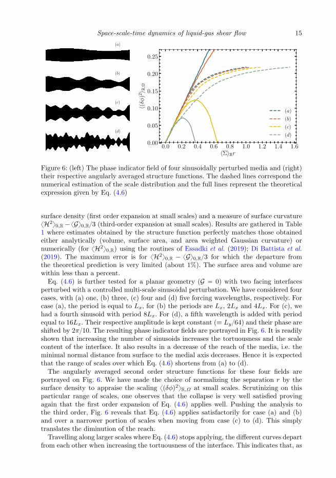
Figure 6: (left) The phase indicator field of four sinusoidally perturbed media and (right)their respective angularly averaged structure functions. The dashed lines correspond thenumerical estimation of the scale distribution and the full lines represent the theoreticalexpression given by Eq. (4.6)

surface density (first order expansion at small scales) and a measure of surface curvaturexH2y0,R ´ xGy0,R3 (third-order expansion at small scales). Results are gathered in Table1 where estimates obtained by the structure function perfectly matches those obtainedeither analytically (volume, surface area, and area weighted Gaussian curvature) ornumerically (for xH2y0,R) using the routines of Essadki et al. (2019); Di Battista et al.(2019). The maximum error is for xH2y0,R ´ xGy0,R3 for which the departure fromthe theoretical prediction is very limited (about 1%). The surface area and volume arewithin less than a percent.Eq. (4.6) is further tested for a planar geometry (G “ 0) with two facing interfaces

perturbed with a controlled multi-scale sinusoidal perturbation. We have considered fourcases, with (a) one, (b) three, (c) four and (d) five forcing wavelengths, respectively. Forcase (a), the period is equal to Lx, for (b) the periods are Lx, 2Lx and 4Lx. For (c), wehad a fourth sinusoid with period 8Lx. For (d), a fifth wavelength is added with periodequal to 16Lx. Their respective amplitude is kept constant (” Ly64) and their phase areshifted by 2π10. The resulting phase indicator fields are portrayed in Fig. 6. It is readilyshown that increasing the number of sinusoids increases the tortuousness and the scalecontent of the interface. It also results in a decrease of the reach of the media, i.e. theminimal normal distance from surface to the medial axis decreases. Hence it is expectedthat the range of scales over which Eq. (4.6) shortens from (a) to (d).The angularly averaged second order structure functions for these four fields are

portrayed on Fig. 6. We have made the choice of normalizing the separation r by thesurface density to appraise the scaling xpδφq2yR,Ω at small scales. Scrutinizing on thisparticular range of scales, one observes that the collapse is very well satisfied provingagain that the first order expansion of Eq. (4.6) applies well. Pushing the analysis tothe third order, Fig. 6 reveals that Eq. (4.6) applies satisfactorily for case (a) and (b)and over a narrower portion of scales when moving from case (c) to (d). This simplytranslates the diminution of the reach.Travelling along larger scales where Eq. (4.6) stops applying, the different curves depart

from each other when increasing the tortuousness of the interface. This indicates that, as


expected, the structure function contains information about the morphology of the mediaunder consideration which differs significantly from case (a) to case (d). We also point outthat increasing the scale content of the interface (the number of sinusoids), results intobroader distributions of xpδφq2yR,Ω. This shows that the second order structure functionhas a great potential for appraising the multi-scale features of heterogeneous media andthus appears a nicely tailored tool for characterizing two-phase flows in particularIn summary, using synthetic fields, we have emphasized a close relationship between

the second-order structure functions at small scales and the geometrical properties ofthe interface (surface area and curvatures). At very large scales, it provides a measure ofliquid volume. At intermediate scales (larger than the reach but smaller than the extentof the typical liquid structures), the structure function provides informations about themorphology of the media and its scale content. Therefore, the reach of the surface plays animportant role here as it separates the range of scales for which geometry applies (viz. Σ,H and G together with Eq. (4.6) are sufficient to describe the media under consideration)and the range of scales for which two-point statistics become a morphological descriptor(Torquato 2002) for which both the geometry and the additional information aboutthe medial axis is required for the structure to be characterized. For scales larger thanthe reach, the separation r should be referred to as the morphological parameter asit is generally done in morphological analysis using e.g. integral geometrical measures(Minkowski functional) of parallel sets (Arns et al. 2004).By virtue of Eq. (2.5), Eq. (4.6) implies

xpδφq2yR,S “3xΣyR r

8

„

1 ´r2

12

ˆ

xH2y0,R ´xGy0,R

3

˙

` Opr5q (4.7)

In Thiesset et al. (2020), it was observed that a prefactor of 13 should be preferablyused in Eq. (4.7) instead of the value of 38. The origin for this difference was notyet explained. By re-analysing the data of Thiesset et al. (2020), it appeared that thisdifference is attributed to the post-processing procedure and particularly an impreciseestimation of spherical averages at small scales. Indeed, in Thiesset et al. (2020), use wasmade of a simple (and computationally light) linear interpolation for transforming two-point statistics from Cartesian to spherical coordinates which was the source of the error.Here, the Radial Basis Function algorithm is used instead with a much more accurateestimation, thereby confirming that the prefactor in Eq. (4.7) is indeed 38.Another difference between the present work and that of Thiesset et al. (2020) is the

scalar field which is employed as being representative of the liquid phase. Thiesset et al.(2020) considered the two-point equation for the liquid-volume-fraction whereas here,the phase indicator is used instead. The latter field can take only 0 or 1 values while theformer can take any value between 0 and 1 in cells containing an interface. When the meshcell size goes to zero, the liquid-volume-fraction tends to the phase indicator. The reasonmotivating the choice for the phase indicator is that comparisons are here made withsome theoretical elaborations (Berryman 1987; Kirste & Porod 1962; Frisch & Stillinger1963) pertaining to porous media, whose description is made on the basis of the phaseindicator but not the (solid) volume fraction. Another argument in favour of the colour-function field is the dependence of the two-point statistics of the liquid-volume-fractionfield to the numerical resolution. For more details on this aspect, the reader is referredto the technical report of Thiesset & Poux (2020).

4.5. Assessment of geometrical measures in the shear-layer

Eq. (4.6) can further be generalized by lifting the spatial average. In this case, xpδφq2yΩis expected to relate to the local values of Σ,H2,G. For the shear layer flow considered


1.0 1.5 2.0tug/Lx

−0.15

−0.10

−0.05

0.00

0.05

0.10

0.15Y/L

y

100

300

500

700

900

1100

1300

1500

1.0 1.5 2.0tug/Lx

80

100

120

140

160

180

〈Σ〉 P

,Y

Figure 7: xΣyP and xΣyP,Y as estimated either from the tesselation of the zero-level surface(dashed grey curve) or from the limit of the second order structure function (full line).The grey dashdotted line in the left figure and the circles in the right figure illustrate thethree typical snaphots used to compute the scale-space budgets.

in the present study, this can be written as

xpδφq2yP,Ω “xΣyP r

2

„

1 ´r2

8

ˆ

xH2y0,P ´xGy0,P

3

˙

` Opr5q (4.8)

where xΣyP, xH2y0,P, xGy0,P which depend on Y and t, are respectively the surface density,the area weighted average of H2 and G within a volume of size LxLz∆y.In Fig. 7, are compared the values of xΣyP as estimated directly from the zero level set

surface (we used the routines described by Essadki et al. 2019; Di Battista et al. 2019)or from the limit to small scales of 2xpδφq2yP,Ωr. The agreement is nearly perfect, withabsolute difference within less than a percent, confirming that Eq. (4.8) holds with a verynice degree of confidence. The agreement is also verified for the spatially average valuesof xΣyP,Y. Again, the difference between the two methods is within a percent (see Fig. 7).Here, the analysis was carried out only for the first order expansion of Eq. (4.8) and didnot incorporate the dependence to the r3 term. The reason is that the flow is populatedby some rather small liquid-structures with small local radius of curvature. Hence, sinceEq. (4.8) is expected to hold up to a separation r2 smaller than the smallest radius ofcurvature, the present numerical resolution was not sufficient for efficiently assessing ther3 scaling of the second-order structure function. This could be done in future work usinga refined simulation.

4.6. Relation to the transport equation of the surface density

Since at small scales, xpδφq2yΩ is proportional to the surface density, the angularaverage of Eq. (2.2a) should approach the transport equation for the surface densitywhen r Ñ 0. The latter was written by Pope (1988); Candel & Poinsot (1990); Drew(1990)

BtΣ ` w ‚ ∇xΣ “ KΣ (4.9)

where K is the stretch rate, which for a liquid-gas interface in an incompressible flowis equal to the tangential strain rate ∇t ¨ ut where ut is the tangential velocity at theinterface and ∇t is the surface gradient (Giannakopoulos et al. 2019). w is the velocityof the interface which is equal to the velocity at the interface u when there is no phasechange. Since σu Ñ u and∇X Ñ ∇x as r Ñ 0, the transfer inX-space tends to u‚∇xΣ,i.e. the convective term in Eq. (4.9). Consequently, the limit towards small scales of the


0.00 0.05 0.10 0.15 0.20 0.25r/Lx

0.00

0.02

0.04

0.06

0.08

0.10〈T

erms〉

Ω,Y×

Lx/u

g[-]

0.00 0.05 0.10 0.15 0.20 0.25r/Lx

0.00 0.05 0.10 0.15 0.20 0.25r/Lx

r-Transfer

Y -Transfer

dt term

RHS

0.00 0.01 0.02

0.00

0.05

0.10

t∗

Figure 8: Angularly and spatially averaged budgets of the total phase indicator fieldfor the three snapshots displayed in Figs. 2 & 7. From left to right: the productionperiod (t˚ “ 0.98), the maximum surface density (t˚ “ 1.37), and the relaxation period(t˚ “ 1.83). The inset represents a closer look at small scales of the r-transfer term.

r-transfer term corresponds to the right hand side of Eq. (4.9). In other words, at smallscales, the transfer term is proportional to the stretch rate K. A similar conclusionswas drawn by Thiesset et al. (2020) using different arguments. This again reinforce theconclusion of Thiesset et al. (2020) that the stretch rate plays for the phase indicatorfield (a non diffusive scalar) the same role as the scalar dissipation rate in diffusive scalarturbulence. Pushing the analysis to the third order, one expects the transport equationfor xH2y ´ xGy3 to be recovered. Hence, the two-point equation for the phase indicatorembed the transport equation for both the surface density and a measure of the surfacecurvatures.

5. Results for the total field

We now explore the contribution of the different terms of the scale/space/time budgetof the total field Eq. (2.3a).

5.1. Spatially and angularly averaged budget

We start by studying the budget after applying the angular (Eq. (2.4)) and spatialaverage (Eq. (2.6)). Recall that by doing so, the different terms have argument list pr, tqand thus light is shed on the scale and time dependence of the transport of liquid. Theinformation about the vertical position within the shear layer and the orientation of theliquid structures is hidden.Results are presented in Fig. 8 for three typical snapshots during the simulation. These

were selected because they are typical of the surface density production period (t˚ “tLxug “ 0.98), the period of maximum surface density (t˚ “ 1.37), and the relaxationperiod (t˚ “ 1.83), respectively (see Figs. 2 & 7).By comparing in Fig. 8 the time-derivative term to the right-hand side of Eq. (2.3a),

it first comes evident that the budget is accurately closed. This is a stringent test whichensures that the simulation resolution and post-processing methods are adequate.A careful examination of Fig. 8 further reveals that, in the range of scales r À 0.15Lx,

the transfer in Y -space is negligible (if not zero) compared to the one in r-space. By

virtue of Eq. (2.7), this is due to the flux xpσv1q pδφq2yP at the plane Y “ ´Lx4 being

almost (if not strictly) equal to the flux at Y “ Lx4. Therefore, over this range of scales,


the angularly and spatially average budget Eq. (2.3a) can be approximated by the oneof an homogeneous flow, the configuration explored by Thiesset et al. (2020). When not

zero, the Y -transfer term is negative meaning that the flux xpσv1q pδφq2yP flowing through

the plane Y “ Lx4 is slightly larger than the one crossing Y “ ´Lx4. In other words,when averaged over the set Y “ tY | ´Ly4 ď Y ď Ly4u, the Y -transfer term evidencesa net transport of liquid in the direction of positive Y , i.e. in the upward direction. Atscales r Á 0.15Lx, the Y -transfer term is of same amplitude as the r-transfer term withopposite signs, and thus the time derivative term tends to zero at large scales. This meansthat the quantity xpδφq2yP,Y,Ω is conserved when r Ñ 8. The same deduction was carriedout in the homogeneous configuration studied by Thiesset et al. (2020).

Let us now focus on the scale/time evolution of the r-transfer term displayed on Fig. 8.This term is found positive over almost the whole range of scales and irrespectively of theinvestigated time. This indicates that, on average, the transfer between the different scalesis directed towards small scales, following a direct cascade mechanism. The r-transferterm peaks at a scale at scale r « 0.03, 0.05, 0.08Lx at time t˚ “ 0.98, 1.37, 1.83,respectively, meaning that the cascade process is maximum at these scales. The timeevolution of the peak location could be related to the increase of the shear layer thickness.However, we do not have yet any physical argument for proving this.

By carefully scrutinizing around r Ñ 0 (see the inset of Fig. 8), it further appears thatthe slope of the r-transfer term which provides information about the stretch rate, ispositive, roughly zero and negative at t˚ “ 0.98, 1.37, 1.83, respectively. This yields atime evolution of xpδφq2yP,Y,Ω at small scales in agreement with the evolution of xΣyP,Ywhere at t˚ “ 0.98 the surface area is increasing, then at t˚ “ 1.37 the surface densityis maximum and finally at t˚ “ 1.83 the surface area starts decreasing (see Fig. 7). Att˚ “ 1.83, the narrow portion of scales (r À 0.02Lx) where the r-transfer term termis negative while larger scales follow a direct cascade mechanism suggests that whilethe largest scales continue transferring the ’energy’ towards the small scales, a smallportion of the smallest scales start relaxing into liquid structures of larger size. Thisinverse cascade mechanism was found to dominate in decaying liquid/gas turbulence(Thiesset et al. 2020) and was attributed to the prominent role of merging and relaxation(e.g. rupture) by capillarity effect of liquid structures. By analogy, it is likely that in theshear-layer, this negative r-transfer at small scales is attributed to the effect of surfacetension which acts in ’sphericalizing’ some elongated liquid structures of typical size lessthan 0.02Lx.

5.2. Angularly averaged budget

We now turn our attention to the evolution of the different terms of Eq. (2.3a) withthe average over the inhomogeneity direction Y being lifted. The dependence to theorientation of the vector r remains hidden by the application of the angular average.The terms now depend on three arguments pY, r, tq. Recall that the centreline of theshear layer is located at Y “ 0. Results are presented again for t˚ “ 0.98, 1.37, 1.83 onFig. 9 and discussed below.

It is again observed that, for the majority of scales and irrespective of t˚, the r-transfer term is positive throughout the shear layer. This means that the cascade ismostly directed towards small scales. The peak is observed at about the same scale asin Fig. 8 and appears to move upward with increasing time, i.e. from about Y “ 0.01Lx

at t˚ “ 0.98 up to Y “ 0.03Lx at t˚ “ 1.83. This is again most likely attributedto the increase of the shear layer thickness. At t˚ “ 1.83, the r-transfer term reveals apocket of negative values around pY, rq « p´0.01Lx, 0.01Lxq. This indicates that the scale


−0.10

−0.05

0.00

0.05

0.10

Y/L

x

−0.10

−0.05

0.00

0.05

0.10

Y/L

x

0.00 0.05 0.10 0.15r/Lx

−0.10

−0.05

0.00

0.05

0.10

Y/L

x

0.00 0.05 0.10 0.15r/Lx

0.00 0.05 0.10 0.15r/Lx

-0.80 -0.40 0.00 0.40 0.80 -0.35 -0.17 0.00 0.17 0.35 -0.20 -0.10 0.00 0.10 0.20

Figure 9: Terms of the angularly averaged budget of the total phase indicator field. Theorange filled contours represent xpδφq2yP,Ω (light to dark correspond to values from 0 to1). The coloured lines correspond to the contours of the different terms normalized byugLx. Positive (negative) values are displayed by full (dashed) lines. From left to right:t˚ “ 0.98, 1.37, 1.83. Top row: r-Transfer term, middle row Y -Transfer term, bottomrow: time derivative term.

distribution close to the centreline undergoes an inverse cascade process. Arguably, thisinverse cascade is consistent with the relaxation mechanism of the interface by capillaryeffect and a diminishing influence of velocity shear which was already identified in Fig.2.

Close to the centreline (Y “ 0), the Y -transfer term is negative meaning that all scales


tend to be convected upwards. The local minimum appears at pY, rq « p0, 0.02Lxq. Onthe contrary, this term appears positive (i.e. downward transport) on both sides of thecentreline. Analysing together the r-transfer and Y -transfer terms reveals an interestingpicture for the scale/space transport of the liquid phase in a turbulent shear layer. Indeed,our analysis suggests that the liquid structures located close to the centreline are firstdominantly convected in the upward direction. Then, once sufficiently pulled away fromthe centreline, these structures start transferring their ’energy content’ predominantly inthe direction of small scales, thereby following a direct cascade process. When these twoprocesses are summed up yields the time derivative of xpδφq2yP,Ω which is negative closeto the centreline and positive on the edge of the shear layer. This observation appliesfor all t˚. This is a key characteristic of the vertical expansion of the shear layer. Thisexpansion is felt by all scales, i.e. it is found that independently of the probed scale, theprobability of crossing an interface (i.e. xpδφq2yP,Ω) is decreasing close to the centrelinewhile it increases on both sides of the centreline. This is readily observed when comparingthe scale distribution xpδφq2yP,Ω from time t˚ “ 0.98 to t˚ “ 1.83.

5.3. Anisotropic scale/space fluxes

We now lift the angular average so that to appraise the full scale/space/time transportof liquid within the shear layer. The different terms of Eq. (2.3a) have now argument listpY, r, tq, i.e. a 5D manifold. Hence, one has to face the difficulty of displaying the resultsin such a large parameter space. An attempt of a possible 3D representation of both thescale distribution xpδφq2yP and energy fluxes pxpδuqpδφq2yP, xpδw1qpδφq2yP, xpσv1qpδφq2yPqin the subset prx, rz , Y, ry “ 0q is given in Fig. 10. This figure exemplifies the verycomplex patterns of liquid transport within the shear layer. The flow appears to be highlyinhomogeneous, with a noticeable dependence of xpδφq2yP and its fluxes to the location Y .Furthermore, the anisotropic character of two-point statistics is striking. Indeed, isotropywould have revealed itself as concentric circles for xpδφq2yP. This is obviously not applyingto the present data. A careful analysis of Fig. 10 further indicate that the streamlinesof energy fluxes are mostly directed towards positive (negative) Y for scales located atpositive (negative) Y , thereby yielding a vertical expansion of the scale distribution. Forpositive Y , the paths of fluxes are directed towards positive (negative) rz suggesting aredistribution of the ’energy’ content in the spanwize direction.Although the 3D representation of two-point statistics provided in Fig. 10 allows

substantiating the complex nature of liquid transport in this particular flow field, a morequantitative analysis is required. For doing this, we made the choice of displaying theresults for only few relevant sub-planes of the full 5D manifold, all all them containing atleast one component in the inhomogeneity directions Y or ry. In Fig. 11, are representedthe contours of xpδφq2yP together with the flux components in the following sub-planes:

‚ the prx, ryq-plane (Y “ rz “ 0) with flux components pxpδuqpδφq2yP, xpδv1qpδφq2yPq,‚ the prx, Y q-plane (ry “ rz “ 0) with flux components pxpδuqpδφq2yP, xpσv1qpδφq2yPq,‚ the pry, Y q-plane (rx “ rz “ 0) with flux components pxpδv1qpδφq2yP, xpσv1qpδφq2yPq.

Note that two-point statistics possesses a central symmetry w.r.t prx, ry, rzq “ p0, 0, 0q.Thus, only the positive half of the abscissae is represented in Fig. 11. The distributionof xpδφq2yP and its respective flux components reveal again the very complex nature ofenergy transfer in this particular flow field. Two-point statistics are strongly dependentto the orientation of the separation vector r (see e.g. the top row of Fig. 11), suggesting avery high degree of anisotropy. The dependence to the location Y within the flow is alsoreadily perceptible (see the middle and bottom row of Fig. 11) meaning that, obviously,inhomogeneity effects are further at play in the shear layer.Firstly, let us focus on the first top row in Fig. 11. For |ry | Á 0.025Lx, the flux


rz

Y

rx

Figure 10: 3D visualisation of the second order structure function in thesubset prx, rz , Y, ry “ 0q at t˚ “ 0.98 (small to large values are displayedby light blue to yellow). The streamlines indicate the path of ’energy’ fluxpxpδuqpδφq2yP, xpδw1qpδφq2yP, xpσv1qpδφq2yPq and are coloured by the magnitude of localfluxes (small to large values: blue to red). The three axis are normalized by Lx. Ainteractive 3D file for this figure is given as supplementary material.

component in the rx direction, i.e. xpδuqpδφq2yP clearly dominates over the one in the rydirection xpδv1qpδφq2yP. This can be largely explained by the strong velocity shear andthus the large difference between the gas and the liquid streamwize velocity. Indeed, theincrement of streamwize velocity δu can be decomposed as δu “ δxuyP ` δu1 while thestatistical symmetry w.r.t the x and z directions implies xvyP “ 0 and thus δv “ δv1

and σv “ σv1. Therefore, for large ry separations, the rx flux dominates over the ryflux because δxuyP « ug " δu1 „ δv1. The top row in Fig. 11 further evidences that forpositive values of ry, the flux components are mostly directed towards positive rx whileby symmetry the opposite is observed for negative values of ry. Consequently, the fluxesin the prx, ryq plane act in distributing the ’energy’ content from the ry component to therx component. Pragmatically speaking, this indicates, due to the velocity shear, liquidstructures will tend to tilt in the clockwise direction. For |ry| À 0.025Lx, the rx and ry-fluxes are of same order of magnitude, and reveal a complex spiralling behaviour which,interestingly, appears rather similar to the one observed for the total kinetic energy inturbulent channel flows Cimarelli et al. (2013).The middle row in Fig. 11 represents the scale distribution xpδφq2yP and fluxes

pxpδuqpδφq2yP, xpσv1qpδφq2yPq in the prx, Y, ry “ 0, rz “ 0q-plane. At t˚ “ 0.98, i.e. duringthe surface production period, the flux in the Y direction dominates over the one in therx direction. This reflects the strong vertical expansion of xpδφq2yP. This is also readilyvisible by comparing the scale distribution xpδφq2yP which appears to spread in the Y

direction from t˚ “ 0.98 to t˚ “ 1.83. This expansion mechanism appears to be roughly


rx/Lx

−0.05

0.00

0.05

r y/L

x

rx/Lx rx/Lx

rx/Lx

−0.05

0.00

0.05

Y/L

x

rx/Lx rx/Lx

0.00 0.05 0.10 0.15ry/Lx

−0.05

0.00

0.05

Y/L

x

0.00 0.05 0.10 0.15ry/Lx

0.00 0.05 0.10 0.15ry/Lx

Figure 11: Iso-values of xpδφq2yP (orange filled contours, from (light) 0 to (dark) 1) andflux components (streamlines coloured by the flux magnitude) in different sub-planesof the full manifold. Top row: prx, ryq-plane, middle row: prx, Y q-plane, bottom row:pry , Y q-plane. Left to right: t˚ “ 0.98, 1.37, 1.83

independent of rx for all scales rx Á 0.025Lx. Still at t˚ “ 0.98, the fluxes amplitudeand direction appear to follow those of the gradient of xpδφq2yP. During the relaxationperiod, i.e. t˚ “ 1.83, and for positive Y , the fluxes are directed towards the direction ofsmaller rx revealing a direct cascade mechanism.The scale distribution xpδφq2yP in the pry, Y, rx “ 0, rz “ 0q-plane together with the

corresponding fluxes pxpδv1qpδφq2yP, xpσv1qpδφq2yPq are portrayed in the bottom row ofFig. 11. Here, xpδφq2yP displays a kind of triangular shape which is characteristic of thestrong inhomogeneity in this particular flow. At t˚ “ 0.98, t˚ “ 1.37 and maybe in a lessobvious manner at t˚ “ 1.83, the magnitude and direction of the fluxes nicely align withthe amplitude and direction of the gradient of xpδφq2yP. Here again, fluxes appears tobe mostly oriented towards smaller scales (direct cascade). pxpδv1qpδφq2yP, xpσv1qpδφq2yPqalso tend to transport xpδφq2yP on both sides of the centreline, i.e. towards positive


0.00 0.05 0.10 0.15 0.20 0.25r/Lx

0.00

0.05

0.10

0.15

〈Terms〉

Ω,Y×Lx/u

g[-]

0.00 0.05 0.10 0.15 0.20 0.25r/Lx

0.00 0.05 0.10 0.15 0.20 0.25r/Lx

r-Transfer

r-Production

Y -Transfer

Y -Production

dt term

RHS

Figure 12: Angularly and spatially averaged budgets for the fluctuating phase indicatorfield. From left to right, t˚ “ 0.98, 1.37, 1.83

(negative) Y for all scales located at planes Y ą 0 (Y ă 0). Consequently, at timeincreases, xpδφq2yP appears to spread over in the Y and ry directions.In summary, Fig. 11 suggests the following picture for the scale/space/time transport

of liquid in the shear layer. The time evolution of the scale distribution xpδφq2yP isfirst affected by a strong contribution of the flux in Y -space which results in verticallyexpanding the two-point statistics towards both side of the shear-layer centreline. Further,the strong velocity shear BY xuyE is responsible for the predominant contribution of the rxflux process and the strong anisotropy of the fluxes in the prx, ryq-plane. The shear ratealso acts in distributing the ’energy’ content from the ry component to the rx component,i.e. liquid structures tend to rotate in the clockwise direction.A last comment is to be made at this stage. In Thiesset et al. (2019a, 2020), it was

shown that the fluxes in scale and physical space can be decomposed into local and non-local interactions. The former (later) indicates that the transfer process occurs betweenadjacent (separate) scales or positions. Here, at several occasions in Fig. 11, it wasemphasized that the paths of local fluxes in the combined physical/scale space matchquite well in direction and amplitude with local gradients of xpδφq2yP. These correspondto the zones where the transfer is mostly local. In such zones, it is worth mentioning thata closure for the fluxes in the form of a diffusion by gradient process can be invoked,with a diffusion coefficient which remains yet to be evaluated. However, there are alsomany regions in the pX, rq-space where local paths of energy do not follow the localgradients of xpδφq2yP. Here, non-local interactions are at play and some other type ofclosure schemes ought to be considered.

6. Results for the fluctuating field

Previous considerations were dedicated to the total phase indicator field φ. However,the present flow configuration reveals a strong statistical inhomogeneity which notablymanifests itself as a significant gradient of the liquid volume fraction xφyP in the Y

direction. However, such an inhomogeneity does not appear explicitly in the equationfor the total field Eq. (2.3a). With the goal of better quantifying its effect, one has topush the analysis to the fluctuating field φ1 “ φ ´ xφyP by using Eq. (2.3b). By doingso, the production terms in the directions Y and ry are made explicit. The latter can beinterpreted as an exchange of energy from the mean field to the randomly fluctuatingfield.


6.1. Spatially and angularly averaged budget

As was done in §5, we start with the spatially and angularly averaged version of Eq.(2.3b) and then progressively go deeper into details by lifting first the spatial averageand then the angular average.The right hand side of the spatially and angularly averaged budget of the fluctuat-

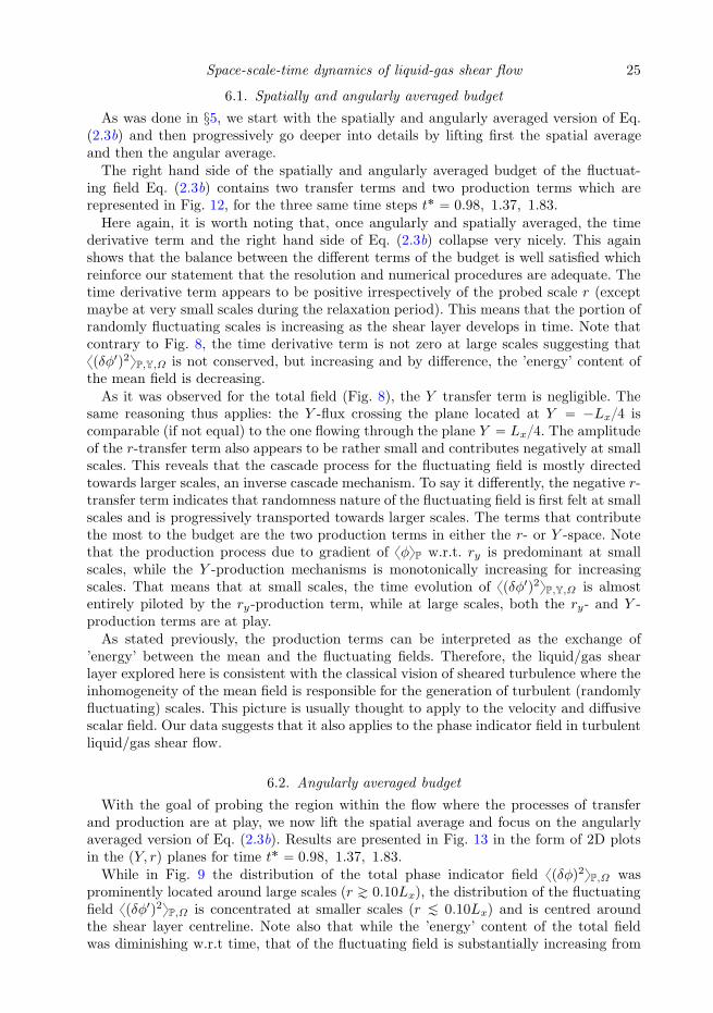
ing field Eq. (2.3b) contains two transfer terms and two production terms which arerepresented in Fig. 12, for the three same time steps t˚ “ 0.98, 1.37, 1.83.Here again, it is worth noting that, once angularly and spatially averaged, the time

derivative term and the right hand side of Eq. (2.3b) collapse very nicely. This againshows that the balance between the different terms of the budget is well satisfied whichreinforce our statement that the resolution and numerical procedures are adequate. Thetime derivative term appears to be positive irrespectively of the probed scale r (exceptmaybe at very small scales during the relaxation period). This means that the portion ofrandomly fluctuating scales is increasing as the shear layer develops in time. Note thatcontrary to Fig. 8, the time derivative term is not zero at large scales suggesting thatxpδφ1q2yP,Y,Ω is not conserved, but increasing and by difference, the ’energy’ content ofthe mean field is decreasing.As it was observed for the total field (Fig. 8), the Y transfer term is negligible. The

same reasoning thus applies: the Y -flux crossing the plane located at Y “ ´Lx4 iscomparable (if not equal) to the one flowing through the plane Y “ Lx4. The amplitudeof the r-transfer term also appears to be rather small and contributes negatively at smallscales. This reveals that the cascade process for the fluctuating field is mostly directedtowards larger scales, an inverse cascade mechanism. To say it differently, the negative r-transfer term indicates that randomness nature of the fluctuating field is first felt at smallscales and is progressively transported towards larger scales. The terms that contributethe most to the budget are the two production terms in either the r- or Y -space. Notethat the production process due to gradient of xφyP w.r.t. ry is predominant at smallscales, while the Y -production mechanisms is monotonically increasing for increasingscales. That means that at small scales, the time evolution of xpδφ1q2yP,Y,Ω is almostentirely piloted by the ry-production term, while at large scales, both the ry- and Y -production terms are at play.As stated previously, the production terms can be interpreted as the exchange of

’energy’ between the mean and the fluctuating fields. Therefore, the liquid/gas shearlayer explored here is consistent with the classical vision of sheared turbulence where theinhomogeneity of the mean field is responsible for the generation of turbulent (randomlyfluctuating) scales. This picture is usually thought to apply to the velocity and diffusivescalar field. Our data suggests that it also applies to the phase indicator field in turbulentliquid/gas shear flow.

6.2. Angularly averaged budget

With the goal of probing the region within the flow where the processes of transferand production are at play, we now lift the spatial average and focus on the angularlyaveraged version of Eq. (2.3b). Results are presented in Fig. 13 in the form of 2D plotsin the pY, rq planes for time t˚ “ 0.98, 1.37, 1.83.While in Fig. 9 the distribution of the total phase indicator field xpδφq2yP,Ω was

prominently located around large scales (r Á 0.10Lx), the distribution of the fluctuatingfield xpδφ1q2yP,Ω is concentrated at smaller scales (r À 0.10Lx) and is centred aroundthe shear layer centreline. Note also that while the ’energy’ content of the total fieldwas diminishing w.r.t time, that of the fluctuating field is substantially increasing from


−0.10

−0.05

0.00

0.05

0.10

Y/L

x

−0.10

−0.05

0.00

0.05

0.10

Y/L

x

−0.10

−0.05

0.00

0.05

0.10

Y/L

x

−0.10

−0.05

0.00

0.05

0.10

Y/L

x

0.00 0.05 0.10 0.15r/Lx

−0.10

−0.05

0.00

0.05

0.10

Y/L

x

0.00 0.05 0.10 0.15r/Lx

0.00 0.05 0.10 0.15r/Lx

-1.30-0.65 0.00 0.65 1.30 -0.50-0.25 0.00 0.25 0.50 -0.25-0.12 0.00 0.12 0.25

Figure 13: Budget of the fluctuating phase indicator field. Orange filled contours representxpδφ1q2yP,Ω (light to dark correspond to values from 0 to 0.5). The coloured linescorrespond to the contours of the different terms normalized by ugLx. Positive (negative)values are displayed by full (dashed) lines. From left to right: t˚ “ 0.98, 1.37, 1.83. Fromtop to bottom: r-Transfer term, r-Production term, Y -Transfer term, Y -Production term,time derivative term.


t˚ “ 0.98 to t˚ “ 1.83. This again reinforces the statement that part of the mean field’energy’ is transferred to the randomly fluctuating field.A careful analysis of Fig. 9 provides further substance and confirms this. Indeed, it

is readily perceived that the contours of xpδφ1q2yP,Ω match almost perfectly those of thery-production term. To a large extent, the time increase in xpδφ1q2yP,Ω is thus due to thisproduction mechanism which further appears to be dominant over the whole extent ofthe shear layer and for almost all scales. In the zones where xpδφ1q2yP,Ω is maximum, thetransfer in both r- and Y -space are negative and also contribute quite significantly tothe budget. In these zones, these two terms thus act in redistributing the energy eithertowards larger scales or in the direction of positive Y , respectively. The production in Y -space does not contribute much, except maybe at rather large scales where it is positive.

The analysis of Fig. 9 allows us to draw the following portray for the scale/spacetransport of the fluctuating liquid field in the shear layer. The driving mechanism is theproduction of fluctuating quantities due to gradient of the mean liquid volume fraction inthe ry direction. ’Energy’ is produced in the zone where inhomogeneities are the largest,here on the centreline of the shear layer. Then, the transfer mechanisms in either scalespace and geometrical space act in redistributing this produced ’energy’ over larger scalesand in the upward direction, respectively. Summing up these different contributions yieldsthe time variations of xpδφ1q2yP,Ω which increases for almost all scales and all verticalpositions within the shear layer. Note that the rate at which xpδφ1q2yP,Ω increases in timeis the highest on both sides of the centreline, in compliance with a vertical enlargementof the shear layer.

6.3. Anisotropic scale/space fluxes

The dependence to the orientation of the separation vector r is now incorporatingto the analysis by lifting the angular average. As in section §5, we selected the samesub-planes of the full 5D manifold:

‚ the prx, ryq-plane (Y, rz “ 0) with flux components pxpδuqpδφ1q2yP, xpδv1qpδφ1q2yPq,‚ the prx, Y q-plane (ry, rz “ 0) with flux components pxpδuqpδφ1q2yP, xpσv1qpδφ1q2yPq,‚ the pry , Y q-plane (rx, rz “ 0) with flux components pxpδv1qpδφ1q2yP, xpσv1qpδφ1q2yPq.

Results are presented in Fig. 14 where both contours of the scale distribution xpδφ1q2yPand streamlines of fluxes in the combined physical/scale space are portrayed. Here again,one is struck by the very complex nature of energy paths in this shear dominated flow.Nevertheless, one can retrieve in Fig. 14 many of the key observations that were drawnpreviously for the angularly averaged budget of the fluctuating liquid field. The mostobvious is probably the increase in the energy content throughout the different sub-planes when time increases from t˚ “ 0.98 to t˚1.83. The scale distribution xpδφ1q2yPappears to evolve mainly towards larger scales and also spread in the vertical direction.By comparing Fig. 11 and Fig. 14, one also recover several common points between thetotal and the fluctuating fields.

Firstly, by scrutinizing the results in the prx, ry, Y “ 0, rz “ 0q-plane, it is clear thatdue to the strong shear, the flux in the rx direction dominates over the one in ry direction.One further observe the same propensity of local fluxes to tilt liquid scales in the clockwisedirection. In the vicinity of the shear layer centreline, one recovers the same spirallingbehaviour.

Secondly, the paths of energy fluxes in the prx, Y, ry “ 0, rz “ 0q-plane in Fig. 14 arevery similar to those observed for the total liquid field in Fig. 11. Here again, one notesa predominant contribution of vertical Y -fluxes which results in a significant verticalexpansion of the scale distribution xpδφ1q2yP. The expansion of xpδφ1q2yPprxq along the


rx/Lx

−0.05

0.00

0.05

r y/L

x

rx/Lx rx/Lx

rx/Lx

−0.05

0.00

0.05

Y/L

x

rx/Lx rx/Lx

0.00 0.05 0.10 0.15ry/Lx

−0.05

0.00

0.05

Y/L

x

0.00 0.05 0.10 0.15ry/Lx

0.00 0.05 0.10 0.15ry/Lx

Figure 14: Iso-values of xpδφ1q2yP (orange filled contours, from (light) 0 to (dark) 0.5) andflux components (streamlines coloured by the flux magnitude) in different sub-planes ofthe full manifold. Top row: prx, ryq-plane, middle row: prx, Y q-plane, bottom row: pry , Y q-plane. Left to right: t˚ “ 0.98, 1.37, 1.83

Y -direction, is readily visible by comparing the results at time t˚ “ 0.98 and t˚ “ 1.83.It appears to be roughly of same amplitude for all scales rx Á 0.025Lx.

Thirdly, the distribution of xpδφ1q2yP in the pry, Y, rx “ 0, rz “ 0q-plane reveals thesame kind of triangular shape as the one of the total field (Fig. 11) except that themaximum values are located in the region where the gradient of xpδφq2yP were thestrongest. Note also that at t˚ “ 0.98 and t˚ “ 1.37, the streamlines of energy fluxesappear to align quite well with the gradient of xpδφ1q2yP. Here again this suggests that, inthis situation, the paths of liquid transport in the combined scale/physical space can bewell approximated by local interactions through a classical diffusion by gradient process.


7. Conclusions

The theoretical framework firstly documented in Thiesset et al. (2020) for a statisti-cally homogeneous flow is here invoked to explore the dynamics of liquid transport in aliquid-gas shear layer, a strongly inhomogeneous flow. The key quantity in this theory isthe second-order structure function of the phase indicator field.

A literature review reveals that this observable is widely employed in other areasof physics dealing with heterogeneous media: e.g. porous media, colloids and fractalaggregates. This vast corpus of research which dates back to the 50’s with the pioneeringwork by e.g. A. Guinier, G. Porod, P Debye, has had a tremendous impact for bettercharacterizing the structure of media which reveals a certain degree of heterogeneity atsome scales. Positioning the problematic of two-phase flows into the wider context ofheterogeneous media has allowed us to highlight the close link between the second-orderstructure function of the phase indicator and some valuable features of the liquid/gasinterface. In particular, the first order expansion for the increments of φ at smallscales relates to the interface surface density, while the third order expansion enablesa combination of the squared mean curvature and Gaussian curvature to be estimated.At intermediate scales, the second-order structure functions behave as a morphologicaldescriptor with r being the morphological parameter. At large scales and under someconditions the liquid volume can also be estimated from two-point statistics.

Most of known theoretical results on the two-point correlation function were obtainedfor homogeneous/isotropic fields. However, two-phase flows generally encountered in realsituations reveal an evolution in a preferential direction due for instance to the presenceof velocity gradients. Therefore there is need to generalize such results to inhomogeneousand anisotropic cases. Following the lines of Berryman (1987), our data suggest thatthe relationship between correlation functions and geometric variables remain true whenanisotropy is coped using an angular average over all orientations of the separation vectorr. It further appears that the homogeneity assumption can further be relaxed, in whichcase the two-point statistics depend on local values of surface area and curvature. Insummary, the results of Kirste & Porod (1962); Frisch & Stillinger (1963) appear tobe possibly generalizable to anisotropic inhomogeneous media. Note though that thisremains yet to be demonstrated and will most likely poses some mathematical difficulties.Indeed, for anisotropic media, one has to consider the dependence to the vector r of auto-correlation functions which is not taken in previous analysis (except by Berryman 1987,who coped with this dependence by using an angular average). For inhomogeneous cases,one has to tackle the dependence of both the auto-correlation function and liquid-volume-fraction to the position vector X which has never been addressed in previous theoreticalwork. However, any progress towards such a generalized expression may have importantrepercussions, not only for treating liquid-gas flows of practical relevance but also forcharacterizing several classes of heterogeneous media.

The analogy between two-phase flows and e.g. porous media breaks down once onerecalls that the liquid phase is a dynamical system. Indeed, contrary to porous mediawhere it is in general relevant to consider a frozen geometry, liquid-gas flows evolve in timethanks to local two-way interactions with the velocity field. In this regard, one of the meritof the present study is to supplement the analysis of two-point statistics with a transportequation which allows to explore the space/scale/time evolution of the liquid phase. Thisframework highlights that the dynamical evolution of the second-order structure functionof the phase indicator is associated with some transfer and production terms which acttogether and concomitantly in a combined scale(r)/physical(X) space. Interestingly, atsmall scales this equation asymptotes the transport equation for the surface density and it


was further evidenced that the transfer in scale space is proportional to the stretch rate atsufficiently small values of r. This is another proof that the stretch rate plays for the phaseindicator the same role as the scalar dissipation rate in ’classical’ scalar turbulence. In itsgeneral formulation, one has to deal with a 7D problem, six dimensions to characterize thedependence to r (anisotropy) and X (inhomogeneity) and one dimension to account forthe time evolution. The liquid-gas shear layer explored in the present work possesses twohomogeneity directions, thereby contracting the problem to a 5 dimensional manifold.A solution for further reducing the problem complexity is then provided by consideringdifferent averaging procedures. More precisely, (i) the dependence to the orientation ofthe separation vector r and physical position Y are first concealed by use of both anangular and spatial average. Then (ii), the dependence to Y is incorporated by liftingthe spatial average before (iii) withdrawing the angular average, thereby allowing theanisotropic character of ’energy’ fluxes to be quantified. We applied this methodologyfor both the total and the fluctuating fields and explored different time steps during thetime evolution of the shear layer, corresponding to the surface area production period,the time of maximum area, and to the relaxation period, respectively.This procedure allowed us to extract some key characteristics of the scale/space/time

transport of liquid in the shear layer, some of which are summarized below.‚ It is first shown that in this particular flow, the total transfer between scales comply

with a direct cascade scenario, where the sense of evolution is directed towards smallscales. The opposite was observed for the fluctuating field suggesting that part of theenergy content of the mean field is transferred to the fluctuating field.

‚ As far as the total phase indicator field is concerned, it was observed that turbulentscales are transported from the centreline towards the edge of the shear layer. As soonas they are sufficiently pulled away, ’energy’ starts being transferred towards smallscales. This observation applies qualitatively for almost all scales and does not changesignificantly during the time evolution of the shear layer, may it lie within the productionor relaxation period.

‚ The fluctuating component of the phase indicator is substantially influenced by thedominant role of production due to gradients of the mean liquid volume fraction. Thery component of the production term is predominant at small scales while the budgetindicates a strong contribution of the ry and Y production processes at larger scales.This indicates that inhomogeneities plays a significant role in the turbulent liquid/gasshear layer.

‚ The very complex nature of liquid transport in the combined scale/physical space isexemplified by quantifying the paths of energy fluxes in some sub-planes of the full 5Dmanifold. The effect of velocity shear appears in a striking manner and manifests itself ina dominant flux in rx direction which causes the tilting of liquid scales in the clockwisedirection. Further, in some regions of the scale/physical space, it was observed that thepaths of energy fluxes align nicely with the gradient of either xpδφq2yP or xpδφ1q2yP. Thisindicates that these zones are driven by some local interactions so that a closure schemeon the basis of a diffusion by gradient process can be formulated. Some other zonesare on the contrary predominantly influenced by non-local interactions which requires adifferent treatment. Further work is needed to better understand the underlying physicsat play for the fluxes to comply with either local or non-local interactions.As an overall conclusion it may be worth recalling that the theoretical framework

invoked here is a descriptive tool which allows scrutinizing the details of liquid transportin both scale and physical space. The theory is not yet predictive, i.e. two-point equationsare not closed since the flux/production terms cannot yet be expressed solely in termsof second-order structure functions of φ or φ1. Consequently, the present paper is rather


observational and intends to document the peculiarities of the phase indicator evolution,a necessary step before providing some physics-informed modelling strategies. In thisregard, we have evidenced that the transfer term in the combined scale/physical spacecan partly be closed by a gradient diffusion process. We also showed theoretically that thetwo-point budget contains informations on the transport of surface density. There thusexists a close link between the present framework and some modelling strategies (e.g.the Eulerian Lagrangian Spray Atomisation model, ELSA see e.g. Lebas et al. (2009);Anez et al. (2019)) which treat liquid/gas flows by use of specific closures for φ and Σ.Second-order structure function of the phase indicator field can also be expressed as afunction of some statistical moments of H and G. Two-point statistics thus share somesimilitude with recent theoretical attempts aiming at generalizing the notion of drop sizedistribution using either Minkowski functional (Thiesset et al. 2019b), or geometricalmetrics and topological invariants (Essadki et al. 2019; Di Battista et al. 2019).Further, although turbulence is by definition a random process and even though

atomization is inherently a local process (pinch-off) which yields discontinuities at finitetime, we conjecture that by using a statistical approach, we can recover some degreeof regularity and predictability for the statistics. The present data appear to confirmthis statement. Indeed, to some extent, the phase indicator field was found to behaverather similarly to a diffusive passive scalar field in single phase turbulence. For instance,the intricate interaction between the randomly fluctuating and mean fields compliesquite well with the classical picture of turbulence in that sense that, at early time inthe shear layer evolution, the scalar ’energy’ is mainly carried by the mean field whichprogressively looses ’energy’ as time increases by feeding the randomly fluctuating partof the φ-field. The analogy between the stretch rate for the phase indicator field and thescalar dissipation rate for ’classical’ scalar turbulence is another example which opens upnice perspectives for modelling purposes.

Acknowledgements

We are thankful to A. Poux, research engineer at CORIA laboratory who wrotethe Fortran kernel for calculating the terms of the scale energy budgets. We are alsograteful to Marc Massot for sharing the routines allowing us to compute the surfacearea and curvatures of iso-level-set surfaces. These are now available through the projectMercur(v)e:. Computations have been carried out in CRIANN (Centre Regional Infor-matique et d’Applications Numeriques de Normandie) under the project 2018002. FTalso benefited from the financial support from the INSIS institute of the CNRS and theCORIA laboratory which are gratefully acknowledged.

Declaration of Interests

The authors report no conflict of interest.

REFERENCES

Adler, PM, Jacquin, Ch G & Quiblier, JA 1990 Flow in simulated porous media. Int. J.Multiphase Flow 16 (4), 691–712.

Anez, J, Ahmed, A, Hecht, N, Duret, B, Reveillon, J & Demoulin, FX 2019 Eulerian–Lagrangian spray atomization model coupled with interface capturing method for dieselinjectors. Int. J. Multiphase Flow 113, 325–342.

: http://docs.mercurve.rdb.is/

http://docs.mercurve.rdb.is/


Arns, Christoph H, Knackstedt, Mark A & Mecke, Klaus R 2004 Characterisation ofirregular spatial structures by parallel sets and integral geometric measures. Colloids andSurfaces A: Physicochemical and Engineering Aspects 241 (1-3), 351–372.

Berryman, James G 1987 Relationship between specific surface area and spatial correlationfunctions for anisotropic porous media. J Math Phys 28 (1), 244–245.

Candel, Sebastien M & Poinsot, Thierry J 1990 Flame stretch and the balance equationfor the flame area. Combust. Sci. Technol. 70 (1-3), 1–15.

Casciola, CM, Gualtieri, P, Benzi, R & Piva, R 2003 Scale-by-scale budget and similaritylaws for shear turbulence. J. Fluid Mech. 476, 105–114.

Ciccariello, S 1995 Integral expressions of the derivatives of the small-angle scatteringcorrelation function. J. Math. Phys. 36 (1), 219–246.

Cimarelli, A, De Angelis, E & Casciola, CM 2013 Paths of energy in turbulent channelflows. J. Fluid Mech. 715, 436–451.

Danaila, L, Antonia, RA & Burattini, P 2004 Progress in studying small-scale turbulenceusing exact two-point equations. New J. Phys. 6 (1), 128.

Debye, P, Anderson Jr, HR & Brumberger, H 1957 Scattering by an inhomogeneous solid.ii. the correlation function and its application. J Appl Phys 28 (6), 679–683.

Di Battista, R, Bermejo-Moreno, I, Menard, T, de Chaisemartin, S & Massot, M2019 Post-processing of two-phase dns simulations exploiting geometrical features andtopological invariants to extract flow statistics: application to canonical objects and thecollision of two droplets. In 10th International Conference on Multiphase Flow, Rio deJaneiro, Brazil .

Drew, Donald A 1990 Evolution of geometric statistics. SIAM J. Appl. Math. 50 (3), 649–666.Duret, B, Luret, G, Reveillon, J, Menard, T, Berlemont, A & Demoulin, FX 2012

DNS analysis of turbulent mixing in two-phase flows. Int. J. Multiphase Flow 40, 93–105.Eggers, J & Villermaux, E 2008 Physics of liquid jets. Rep Prog Phys 71 (3), 036601.Essadki, M, Drui, F, Larat, A, Menard, T & Massot, M 2019 Statistical modeling of

the gas–liquid interface using geometrical variables: Toward a unified description of thedisperse and separated phase flows. Int. J. Multiphase Flow 120, 103084.

Federer, H 1959 Curvature measures. Transactions of the American Mathematical Society93 (3), 418–491.

Fedkiw, R P, Aslam, T, Merriman, B & Osher, S 1999 A non-oscillatory eulerian approachto interfaces in multimaterial flows (the ghost fluid method). J Comput Phys 152 (2),457–492.

Fitzhugh, R 1983 Statistical properties of the asymmetric random telegraph signal, withapplications to single-channel analysis. Math. Biosci. 64 (1), 75–89.

Frisch, HL & Stillinger, FH 1963 Contribution to the statistical geometric basis of radiationscattering. J. Chem. Phys. 38 (9), 2200–2207.

Fuster, D, Matas, J-P, Marty, S, Popinet, S, Hoepffner, J, Cartellier, A & Zaleski,S 2013 Instability regimes in the primary breakup region of planar coflowing sheets. J.Fluid Mech. 736, 150–176.

Gatti, D, Remigi, A, Chiarini, A, Cimarelli, A & Quadrio, M 2019 An efficient numericalmethod for the generalised kolmogorov equation. J. Turbul. 20 (8), 457–480.

Giannakopoulos, G K, Frouzakis, C E, Mohan, S, Tomboulides, A G & Matalon,M 2019 Consumption and displacement speeds of stretched premixed flames-theory andsimulations. Combust. Flame 208, 164–181.

Gorokhovski, Mikhael & Herrmann, Marcus 2008 Modeling primary atomization. Annu.Rev. Fluid Mech. 40, 343–366.

Grimson, Malcolm J 1983 Small-angle scattering from colloidal dispersions. J. Chem. Soc.79 (6), 817–832.

Hill, RJ 2002 Exact second-order structure-function relationships. J. Fluid Mech. 468, 317–326.

Kirste, R & Porod, G 1962 Rontgenkleinwinkelstreuung an kolloiden systemenasymptotisches verhalten der streukurven.Kolloid-Zeitschrift und Zeitschrift fur Polymere184 (1), 1–7.

Lasheras, Juan C & Hopfinger, EJ 2000 Liquid jet instability and atomization in a coaxialgas stream. Annu Rev Fluid Mech 32 (1), 275–308.


Lebas, R, Menard, T, Beau, PA, Berlemont, A & Demoulin, FX 2009 Numericalsimulation of primary break-up and atomization: DNS and modelling study. Int. J.Multiphase Flow 35 (3), 247–260.

Ling, Y, Fuster, Daniel, Tryggvason, G & Zaleski, S 2019 A two-phase mixing layerbetween parallel gas and liquid streams: multiphase turbulence statistics and influence ofinterfacial instability. J. Fluid Mech. 859, 268–307.

Ling, Y, Fuster, D, Zaleski, S & Tryggvason, G 2017 Spray formation in a quasiplanargas-liquid mixing layer at moderate density ratios: a numerical closeup. Phys. Rev. Fluids2 (1), 014005.

Marati, N, Casciola, CM & Piva, R 2004 Energy cascade and spatial fluxes in wallturbulence. J. Fluid Mech. 521, 191–215.

Marmottant, Ph & Villermaux, E 2004 On spray formation. J Fluid Mech 498, 73–111.Menard, T, Tanguy, S & Berlemont, A 2007 Coupling level set/VOF/ghost fluid methods:

Validation and application to 3D simulation of the primary break-up of a liquid jet. Int.J. Multiphase Flow 33 (5), 510–524.

Moran, J., Fuentes, A, Liu, F & Yon, J 2019 Fracval: An improved tunable algorithmof cluster-cluster aggregation for generation of fractal structures formed by polydisperseprimary particles. Computer Physics Communications 239, 225–237.

Pope, SB 1988 The evolution of surfaces in turbulence. Int J Eng Sci 26 (5), 445–469.Portela, FA, Papadakis, G & Vassilicos, JC 2017 The turbulence cascade in the near wake

of a square prism. J. Fluid Mech. 825, 315–352.Pumir, A 1996 Turbulence in homogeneous shear flows. Phys. Fluids 8 (11), 3112–3127.Rosti, ME, Ge, Z, Jain, SS, Dodd, MS & Brandt, L 2019 Droplets in homogeneous shear

turbulence. J. Fluid Mech. .Rudman, M 1998 A volume-tracking method for incompressible multifluid flows with large

density variations. Int J Numer Methods Fluids 28 (2), 357–378.Sorensen, CM 2001 Light scattering by fractal aggregates: a review. Aerosol Science &

Technology 35 (2), 648–687.Sussman, M, Smith, KM, Hussaini, MY, Ohta, M & Zhi-Wei, R 2007 A sharp interface

method for incompressible two-phase flows. J Comput Phys 221 (2), 469–505.Taguelmimt, N, Danaila, L & Hadjadj, A 2016 Effects of viscosity variations in temporal

mixing layer. Flow, Turbulence and Combustion 96 (1), 163–181.Thiesset, F, Dumouchel, C & Menard, T 2019a A new theoretical framework for

characterizing the transport of liquid in turbulent two-phase flows. In ILASS-Europe,Paris.

Thiesset, F, Dumouchel, C, Menard, T, Aniszewski, W, Vaudor, G & Berlemont, A2019b Probing liquid atomization using probability density functions, the volume-basedscale distribution and differential geometry. In ILASS-Europe, Paris.

Thiesset, F, Duret, B, Menard, T, Dumouchel, C, Reveillon, J & Demoulin, FX 2020Liquid transport in scale space. J. Fluid Mech. 886.

Thiesset, F. & Poux, A. 2020 Numerical assessment of the two-point statistical equationsin liquid/gas flows. Tech. Rep.. CNRS, Normandy Univ., UNIROUEN, INSA Rouen,CORIA. Available at https://hal.archives-ouvertes.fr/hal-02614565.

Torquato, S. 2002 Random Heterogeneous Materials. Microstructure and MacroscopicProperties. Springer-Verlag New York.

Vaudor, G, Menard, T, Aniszewski, W, Doring, M & Berlemont, A 2017 A consistentmass and momentum flux computation method for two phase flows. application toatomization process. Computers Fluids 152, 204–216.

Wu, H-I & Schmidt, PW 1971 Intersect distributions and small-angle X-ray scattering theory.J. Appl. Crystallogr. 4 (3), 224–231.

Yeung, PK, Donzis, DA & Sreenivasan, KR 2005 High-reynolds-number simulation ofturbulent mixing. Phys. Fluids 17 (8), 081703.

Zhang, J 1996 Acceleration of five-point red-black gauss-seidel in multigrid for poisson equation.Appl. Math. Comput. 80 (1), 73–93.

https://hal.archives-ouvertes.fr/hal-02614565

Documents

Space-scale-time dynamics of liquid–gas shear flow