SP-CNN: A Scalable and Programmable CNN-based Accelerator ASPLOS 2015.pdfCNN Cell Each cell is a dynamical system with an input, output, and a state that evolves according to some

SP-CNN: A Scalable and Programmable CNN-based Accelerator

Dilan Manatunga

Dr. Hyesoon Kim

Dr. SaibalMukhopadhyay

Motivation

Power is a first-order design constraint, especially for embedded devices.

Certain applications prevalent in embedded devices

Image processing, audio processing, context awareness, etc.

Trend of including more specialized, energy-efficient accelerators.

Moto X 2013

Cellular Neural Networks

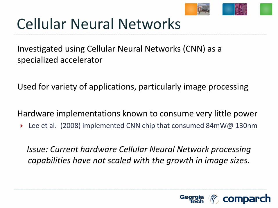
Investigated using Cellular Neural Networks (CNN) as a specialized accelerator

Used for variety of applications, particularly image processing

Hardware implementations known to consume very little power

Lee et al. (2008) implemented CNN chip that consumed 84mW@ 130nm

Issue: Current hardware Cellular Neural Network processing capabilities have not scaled with the growth in image sizes.

Outline

Cellular Neural Network (CNN) Background

Multiplexing

SP-CNN Architecture

Results

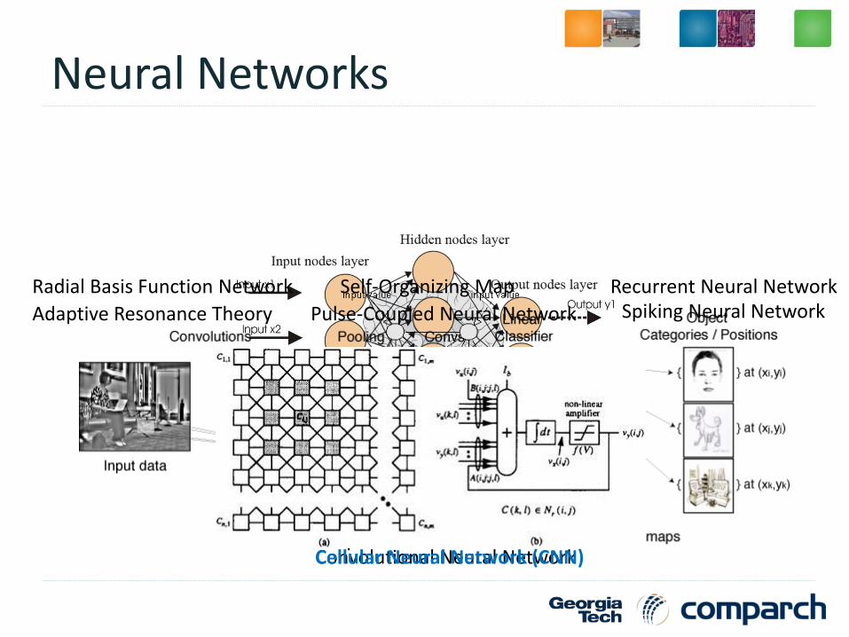
Neural Networks

Artificial Neural Network

Convolutional Neural NetworkHopfield Neural Network

Radial Basis Function Network Self-Organizing Map Recurrent Neural Network

Adaptive Resonance Theory Pulse-Coupled Neural Network Spiking Neural Network

Cellular Neural Network (CNN)

CNN Background

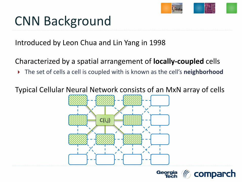
Introduced by Leon Chua and Lin Yang in 1998

Characterized by a spatial arrangement of locally-coupled cells

The set of cells a cell is coupled with is known as the cell’s neighborhood

Typical Cellular Neural Network consists of an MxN array of cells

C(i,j)

CNN Applications

Image Processing Edge Detection, Image Segmentation, Movement Detection, etc.

Pattern Recognition

Associative Memory

Solving Partial Differential Equations

Pre-data processing for other neural networks

CNN Universal Machine is Turing Complete

CNN Cell

Each cell is a dynamical system with an input, output, and a state thatevolves according to some prescribed laws.

Most CNNs follow the standard CNN state and output equations:𝑑𝑥𝑖𝑗(𝑡)

𝑑𝑡= −𝑥𝑖𝑗 𝑡 +

𝐶 𝑘,𝑙 ∈𝑁𝑟 𝑖,𝑗

𝑎𝑘𝑙 ∗ 𝑦(𝑡)𝑘𝑙 +

𝐶 𝑘,𝑙 ∈𝑁𝑟 𝑖,𝑗

𝑏𝑘𝑙 ∗ 𝑢𝑘𝑙 + 𝑧

𝑦𝑖𝑗 𝑡 =1

2𝑥𝑖𝑗 𝑡 + 1 − 𝑥𝑖𝑗 𝑡 − 1

𝑁𝑟 𝑖, 𝑘 represents neighborhood for cell at location i,j

x represents the current state

y is the cell outputs

u is the cell inputs

z is the threshold value

a and b are the feed-forward and feedback weights

Digital CNN Cell

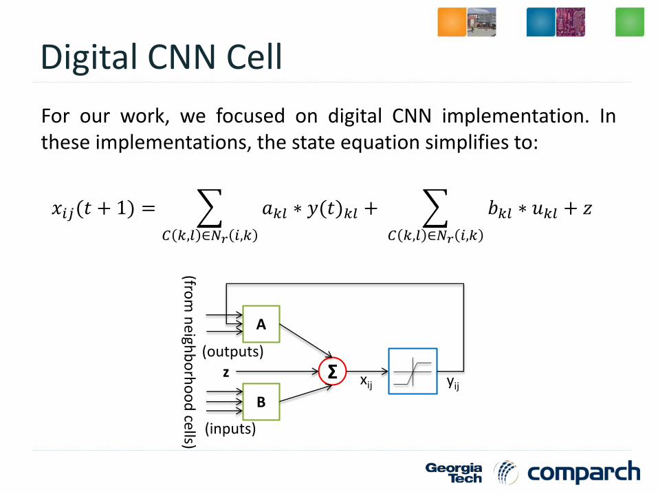
For our work, we focused on digital CNN implementation. Inthese implementations, the state equation simplifies to:

𝑥𝑖𝑗(𝑡 + 1) =

𝐶 𝑘,𝑙 ∈𝑁𝑟 𝑖,𝑘




A

B

Σz(outputs)

(inputs)

xij yij

(from

ne

ighb

orh

oo

d cells)

CNN Gene

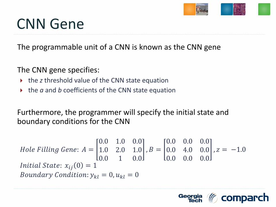
The programmable unit of a CNN is known as the CNN gene

The CNN gene specifies: the z threshold value of the CNN state equation

the a and b coefficients of the CNN state equation

Furthermore, the programmer will specify the initial state and boundary conditions for the CNN

𝐻𝑜𝑙𝑒 𝐹𝑖𝑙𝑙𝑖𝑛𝑔 𝐺𝑒𝑛𝑒: 𝐴 =0.0 1.0 0.01.0 2.0 1.00.0 1 0.0

, 𝐵 =0.0 0.0 0.00.0 4.0 0.00.0 0.0 0.0

, 𝑧 = −1.0

𝐼𝑛𝑖𝑡𝑖𝑎𝑙 𝑆𝑡𝑎𝑡𝑒: 𝑥𝑖𝑗 0 = 1

𝐵𝑜𝑢𝑛𝑑𝑎𝑟𝑦 𝐶𝑜𝑛𝑑𝑖𝑡𝑖𝑜𝑛: 𝑦𝑘𝑙 = 0, 𝑢𝑘𝑙 = 0

Example Application

The following is an example of running the HoleFilling gene, an application commonly used in character recognition, on a input image of the number eight.

Hardware CNNs

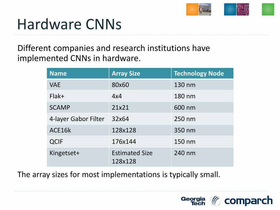
Different companies and research institutions have implemented CNNs in hardware.

The array sizes for most implementations is typically small.

Name Array Size Technology Node

VAE 80x60 130 nm

Flak+ 4x4 180 nm

SCAMP 21x21 600 nm

4-layer Gabor Filter 32x64 250 nm

ACE16k 128x128 350 nm

QCIF 176x144 150 nm

Kingetset+ Estimated Size 128x128

240 nm

Issue: Image Dim vs CNN Array Dim

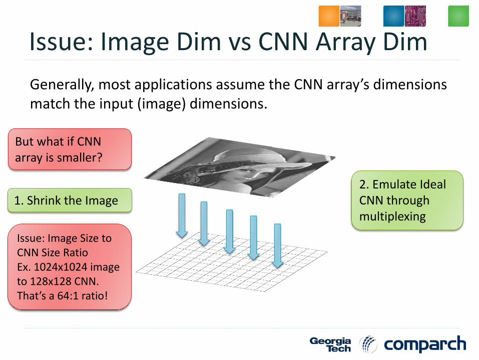
Generally, most applications assume the CNN array’s dimensions match the input (image) dimensions.

But what if CNN array is smaller?

1. Shrink the Image

Issue: Image Size toCNN Size RatioEx. 1024x1024 image to 128x128 CNN.That’s a 64:1 ratio!

2. Emulate Ideal CNN through multiplexing

Partition 1 CNN StateT=0




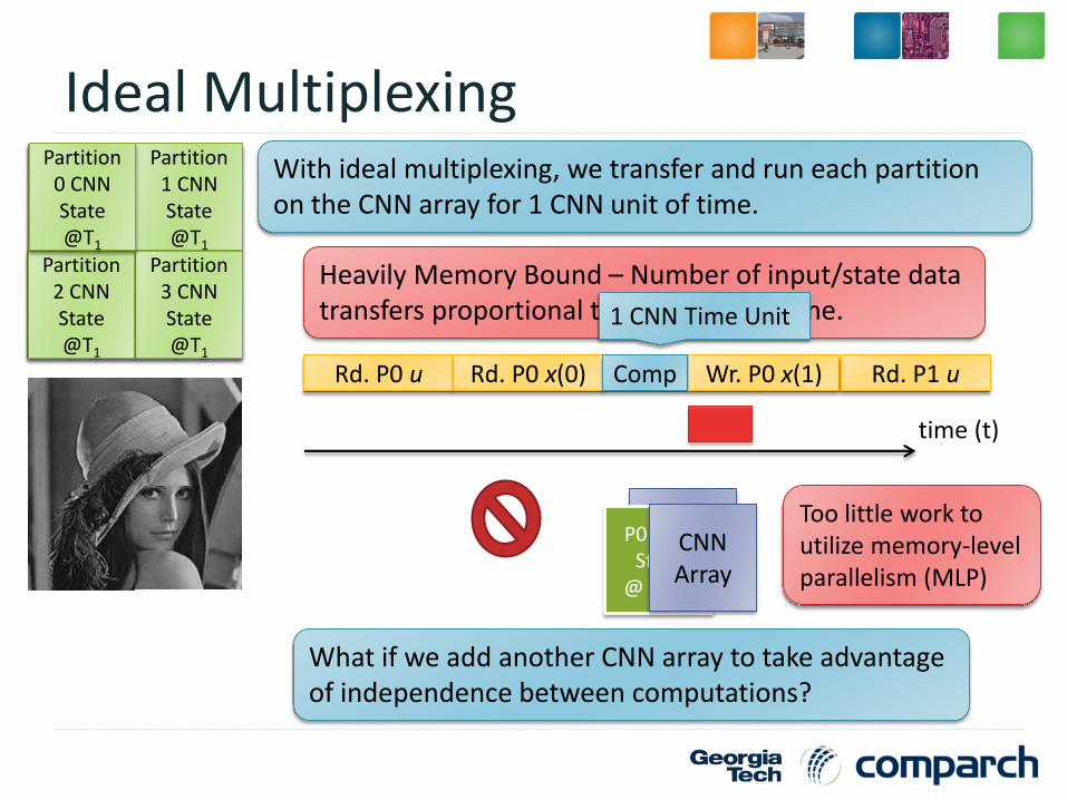
Ideal MultiplexingWith ideal multiplexing, we transfer and run each partition on the CNN array for 1 CNN unit of time.

Heavily Memory Bound – Number of input/state data transfers proportional to convergence time.

Partition 1 CNN State@T1



Rd. P0 u Rd. P0 x(0) Comp Wr. P0 x(1)


time (t)

What if we add another CNN array to take advantage of independence between computations?

Too little work to utilize memory-level parallelism (MLP)

Rd. P1 u

CNN Array

P0 CNN State

@ T1+1

CNN Array

1 CNN Time Unit

Key-Insight

Let’s take advantage of CNNs ability to still converge to thecorrect solution in presence of small errors.

So, instead of running for partition on CNN array for 1 unit time,run partition for an interval T >> 1 unit of time.

This is the key insight to our Scalable and Programmable CNN(SP-CNN) architecture.

SP-CNN Multiplexing

With SP-CNN multiplexing, we run each partition on the CNN array for a certain interval of time.

Run for 1 CNN Unit of Time

Run for INTERVAL CNN unit of TimeRd. P0 u Rd. P0 x(0) Comp Wr. P0 x(1)

Rd. P0 u Rd. P0 x(0) Comp (INTERVAL=4) Wr. P0 x(1)

time (t)

1st iteration

interval

2nd iteration

cnn-time (t)4 8 12 16 20 24 28 320

SP-CNNINTERVAL=4

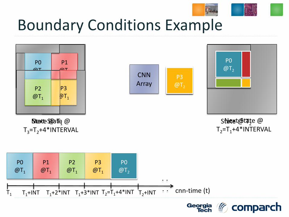
Boundary Conditions

When running a partition on the CNN array, what should we set boundary conditions to?

To ensure that information propagates between partitions, we set the boundary condition for a given partition to its neighboring cells.

Partition 0 Pixel

Partition 1 Pixel

Partition 0 Boundary Pixel

Partition 0 Boundary made of Partition 1 Data

True Boundary Condition for Image

Partition 0 Boundary also part of True Boundary

Image Pixel

True Boundary Cond.

P0@T1

P1@T1

P2@T1

P3@T1

Boundary Conditions Example

CNN Array

State @ T1 Next-State @ T2=T1+4*INTERVAL

cnn-time (t)T1+INTT1

P0@T1

P1@T1

P2@T1

P3@T1

T1+2*INT T1+3*INT T2=T1+4*INT

P0@T2

P1@T1

P0@T1

P3@T1

P1@T2P2

@T1

P2@T2

P3@T2

P0@T2

T2+INT

P0@T2

Next-State @ T3=T2+4*INTERVAL

State @ T2

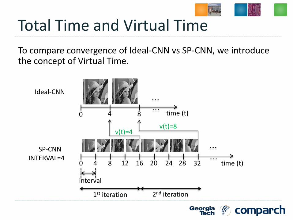
Total Time and Virtual Time

To compare convergence of Ideal-CNN vs SP-CNN, we introduce the concept of Virtual Time.

1st iteration

interval

2nd iteration

time (t)4 8 12 16 20 24 28 320

v(t)=4v(t)=8

time (t)4 80

Ideal-CNN

SP-CNNINTERVAL=4

Reduced Memory Transfers

If virtual convergence time does not significantly increase in the SP-CNN case, we can significantly reduce number of memory transfers.

Ideal-CNN

Virtual Convergence Time (t)1 2 3 4 5 6 7 80

P0 P1 P2 P3 P0 P1 P2 P3

T-4 T-2 T-2 T-1 T

P0 P1 P2 P3

Virtual Convergence Time (t)

1 2 3 4 5 6 7 80

P0 P1

T2-4 T2-3 T2-2 T2-1 T2

P3SP-CNNINTERVAL=4

T Memory Transfers

T2/INTERVAL Memory Transfers

If T≅T2, than memory transfers reduced by factor of about 1/INTERVAL.

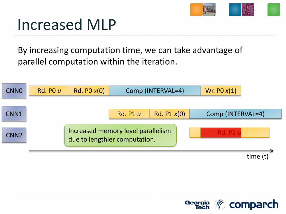
Increased MLP

By increasing computation time, we can take advantage of parallel computation within the iteration.

time (t)

Rd. P0 u Rd. P0 x(0) Comp (INTERVAL=4) Wr. P0 x(1)CNN0

Rd. P1 u Rd. P1 x(0) Comp (INTERVAL=4)CNN1

CNN2 Rd. P2 uIncreased memory level parallelism due to lengthier computation.

SP-CNN Architecture

Global memory • Stores the input

and cnn state.

CNN-P• CNN processing

unit. • Processes

partition

Scheduler• Assigns partitions

to CNN-P

Host Processor• Sends work to

SP-CNN

Methodology

6 benchmarks with 10 input images.

The test images are of size 1024x1024 (~720p) or 2048x2048 (~1440p)

*Local applications are essentially simple convolution operations that only care about neighborhood values.

Name Mechanism

Ideal CNN array size equal to Image Size

SP-CNN Proposed architecture

Application Type

Corner Detection Local*

Edge Detection Local*

Connected Component Global

Hole Filling Global

Rotation Detector Global

Shadow Creator Global

Simulators

Functional Simulator Specifications

CNN Array Size = 128x128

Interval Time = 128 cnn time units

Timing simulator (DRAMSim2 for memory)

CNN timing parameters based on VAE architecture* (200Mhz @ 130nm)

1 Processing Element for 32 cells

Each CNN-P unit has 64 MSHR entries. (Based off Nvidia Fermi)

Used 2GB DRAM memory with DDR3 timing parameters.

*VAE is an existing hardware CNN chip implementation [Lee et. Al 2008]

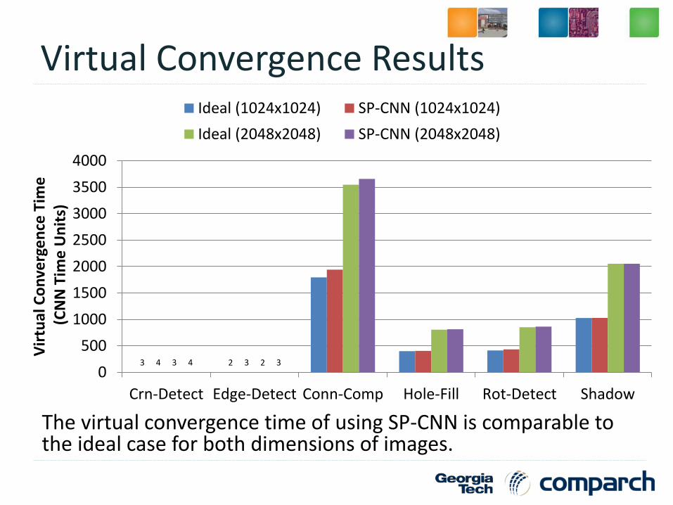
Virtual Convergence Results

The virtual convergence time of using SP-CNN is comparable to the ideal case for both dimensions of images.

3 24 33 24 3

0

500

1000

1500

2000

2500

3000

3500

4000

Crn-Detect Edge-Detect Conn-Comp Hole-Fill Rot-Detect Shadow

Vir

tual

Co

nve

rge

nce

Tim

e(C

NN

Tim

e U

nit

s)

Ideal (1024x1024) SP-CNN (1024x1024)

Ideal (2048x2048) SP-CNN (2048x2048)

Timing Results for 1024x1024

Meet 60 FPS for most applications when CNN-P = 1

Meet 60 FPS for all applications when CNN-P = 8

0

16

32

48

64

80

96

112

128


Tim

e (

ms) CNN-P=1

CNN-P=2

CNN-P=4

CNN-P=830 FPS Boundary

60 FPS Boundary

Timing Results for 2048x2048

Meet 30 FPS for most applications when CNN-P=8 60 FPS difficult to meet even with CNN-P=8

0

16

32

48

64

80

96

112

128


Tim

e (

ms) CNN-P=1

CNN-P=2

CNN-P=4

CNN-P=830 FPS Boundary

60 FPS Boundary

375 195

Future Work

Try more computationally-intensive CNN applications

Video processing, Face recognition, pattern recognition, etc.

FPGA implementation of SP-CNN Will allow us to perform better performance and power comparisons

against CPU, GPU, etc.

Further SP-CNN optimizations Determine optimal interval values

Boundary Condition Propagation Time

Determine if a CNN gene is suitable for SP-CNN

Conclusion

Our proposed SP-CNN architecture brings scalability to small sized hardware CNN arrays.

SP-CNN shows performance that is comparable to the ideal case in terms of virtual convergence time.

Energy consumption around 10 to 30 mJ.

SP-CNN can meet 30 FPS and 60 FPS standards for most benchmarks. This can further improved with better scaling of the CNN technology.

Questions?

31

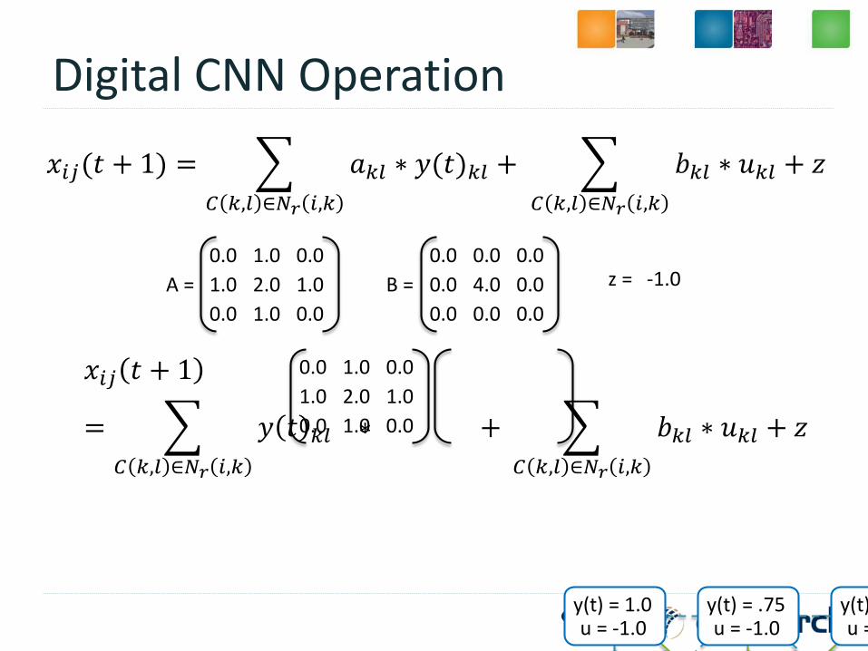
Digital CNN Operation

0.0 0.0 0.0

0.0 4.0 0.0

0.0 0.0 0.0

B = z = -1.0

𝑥𝑖𝑗(𝑡 + 1) =





y(t) = 1.0u = -1.0

y(t) = .75u = -1.0

y(t) = 1.0u = -

0.0 1.0 0.0

1.0 2.0 1.0

0.0 1.0 0.0

A =

𝑥𝑖𝑗 𝑡 + 1

=


𝑦 𝑡 𝑘𝑙 ∗ +



0.0 1.0 0.0

1.0 2.0 1.0

0.0 1.0 0.0

33

The basis of the CNN operation is that we eventually converge to the correct solution.

However, there are no guarantees on the convergence time and different inputs can converge at different rates.

0%

10%

20%

30%

40%

50%

60%

70%

80%

90%

100%

1

26

51

76

10

1

12

6

15

1

17

6

20

1

22

6

25

1

27

6

30

1

32

6

35

1

37

6

40

1

42

6

45

1

47

6

50

1

52

6

55

1

57

6

60

1

62

6

65

1

67

6

70

1

72

6

75

1

77

6

80

1

Output Error of Running HoleFilling Gene on a CNN for Various 1024x1024 Test Images

capitalA

circle

eight

filledSquare

lowerA

nine

rect

seven

vertLine

zero

34

Slow Propagation

Updated information in boundary conditions is seen at the beginning of the next iteration

y(0) y(0)’s output

y(0)’s output

partition 0

partition 1

y(0)

y(1)

y(1)

1 2

3 4

5

6

35

The SP-CNN algorithm can be viewed below:

while change do

change = false

for p in partitions do

loadStateAndInputToCNN(p)

for n = 0; n < interval; n++, t++ do

change |= parallel-computation of state

parallel-computation of output

end for

saveToNextStateFromCNN(p)

end for

swapStateAndNextStatePointers(p)

iter += 1, vt += interval

end while

36

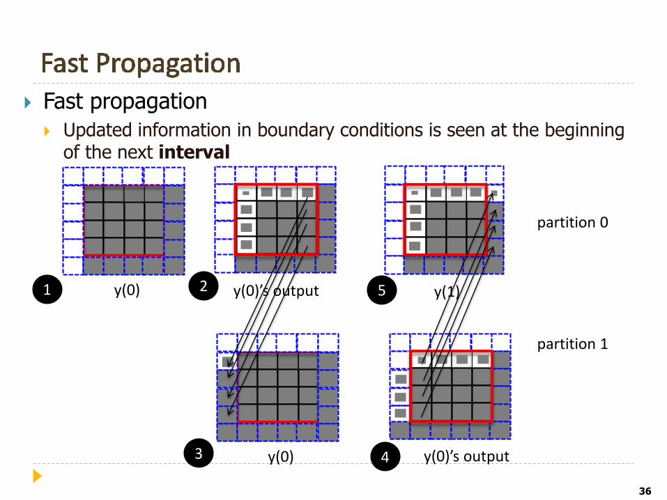
Fast propagation

Updated information in boundary conditions is seen at the beginning of the next interval

y(0) y(0)’s output y(1)

y(0) y(0)’s output

partition 0

partition 1

1

3

2

4

5

37

Using fast propagation, the partition order can improve onprogram convergence time.

For example, if data is passed through the cells from right to left, thenwe can converge faster by moving through partitions in a reversecolumn-major order.

Partition ordering only matters if fast propagation used.

38

For Connected Component, Hole Filling, and Rotation Detector, fast propagation can provide an average speedup from 15% to 30%.

Shadow Creator shows no benefit since the information propagation in that benchmark is from right-to-left.

00.10.20.30.40.50.60.70.80.9

11.11.21.31.41.5


Avg

. Sp

ee

du

p i

n

Tota

l Co

nve

rge

nce

Tim

e

1024x1024 2048x2048

39

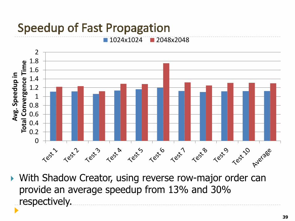
With Shadow Creator, using reverse row-major order can provide an average speedup from 13% and 30% respectively.

00.20.40.60.8

11.21.41.61.8

2

Avg

. Sp

ee

du

p in

To

tal C

on

verg

en

ce T

ime

1024x1024 2048x2048

40

Virtual Convergence Time

Originally: 𝑣𝑖𝑟𝑡𝑢𝑎𝑙𝐶𝑜𝑛𝑣𝑇𝑖𝑚𝑒 = 𝑛 ∗ 𝑇, where N is the number of iterations

Now: 𝑣𝑖𝑟𝑡𝑢𝑎𝑙𝐶𝑜𝑛𝑣𝑇𝑖𝑚𝑒 = 𝑖=1𝑛 min(𝑇,max(∀𝑝∈𝑃𝑎𝑟𝑡𝑖𝑡𝑖𝑜𝑛𝑠𝑐𝑜𝑛𝑣𝑇𝑖𝑚𝑒(𝑝, 𝑖)))

convTime(p, i) is the convergence time for partition p during iteration i

41

Both naïve mechanisms show errors on average of 20%, with max errors as high as 90% for global applications.

Local type applications only show error for the No-Share mechanisms.

SP-CNN converged correctly to solution for all benchmarks and tests.

0%

20%

40%

60%

80%

100%


Pe

rce

nt

Erro

r

No-Share Avg. Error Share Avg. Error

No-Share Max. Error Share Max. Error

42

For the global applications, memory bandwidth contention decreases the ability to achieve linear scaling.

Shadow shows very poor scaling since many of the partitions converge quickly, therefore the CNN occupation time is low.

0

1

2

3

4

5

6

Crn-Detect Edge-Detect Conn-Comp Hole-Fill Rot-Detect ShadowAvg

. Exe

cuti

on

Tim

e S

pe

ed

up

CNN-P=2 (1024x1024) CNN-P=4 (1024x1024) CNN-P=8 (1024x1024)

CNN-P=2 (2048x2048) CNN-P=4 (2048x2048) CNN-P=8 (2048x2048)

43

Prefetching only provides some benefits when the number of CNN-Ps is equal to 1.

When the number of CNN-Ps scales up, than the memory bandwidth contention becomes too large, and prefetching can actually cause slowdowns.

0

0.2

0.4

0.6

0.8

1

1.2

1.4

1.6

1.8

2

1 2 4 8

Avg

. Exe

cuti

on

Tim

e S

pe

ed

up

Number of CNN-P

Crn-Detect

Edge-Detect

Conn-Comp

Hole-Fill

Rot-Detect

Shadow

44

We also evaluated our SP-CNN mechanisms over CPU and GPU implementations of the benchmarks.

For two benchmarks, Hole-Filling and Rotation Detector, we could not easily develop a CPU/GPU algorithm, so we collect their timing results by emulating the CNN’s operation on the corresponding platform.

Name Model Power Frequency Technology

CPU Intel® Core ™ i5-35550

77W (TDP) 3.3 GHz 22nm

GPU NVIDIA K1 mobile

1.5W 900 MHz 28nm

SP-CNN 0.73mW per PE, 35.6 uWper node

200 MHz 45nm

45

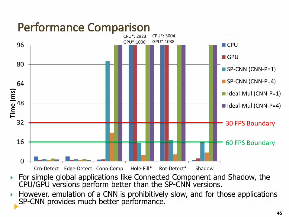
For simple global applications like Connected Component and Shadow, the CPU/GPU versions perform better than the SP-CNN versions.

However, emulation of a CNN is prohibitively slow, and for those applications SP-CNN provides much better performance.

0

16

32

48

64

80

96

Crn-Detect Edge-Detect Conn-Comp Hole-Fill* Rot-Detect* Shadow

Tim

e (

ms)

CPU

GPU

SP-CNN (CNN-P=1)

SP-CNN (CNN-P=4)

Ideal-Mul (CNN-P=1)

Ideal-Mul (CNN-P=4)

60 FPS Boundary

30 FPS Boundary

CPU*: 2923 GPU*:1006

CPU*: 3004 GPU*:1038

46

For Connected Component and Shadow, execution time dominates over the low power consumption of SP-CNN, causing overall energy to be larger than the GPU case.

Hole-Filling and Rotation Detector do show cases where the SP-CNN can perform complex tasks at a low energy cost.

0

10

20

30

40

50

60

Crn-Detect Edge-Detect Conn-Comp Hole-Fill* Rot-Detect* Shadow

Ene

rgy

(mJ)

CPU GPU SP-CNN (CNN-P=1) SP-CNN (CNN-P=4)

Optimization: Early-Finish

Originally, each partition run for on the CNN for the entire interval time T.

We saw cases where a partition converged on the CNN before interval finished.

Rest of execution essentially does nothing.

So, introduced Early-Finish, where a partition runs on the CNN till it either converges or interval time T is reached.

Documents

SP-CNN: A Scalable and Programmable CNN-based Accelerator ASPLOS 2015.pdfCNN Cell Each cell is a dynamical system with an input, output, and a state that evolves according to some