Southern Annular Mode Dynamics in Observations and Models ... · Southern Annular Mode Dynamics in Observations and Models. Part II: Eddy Feedbacks ISLA R. SIMPSON Department of Physics,

Southern Annular Mode Dynamics in Observations and Models. Part II:Eddy Feedbacks

ISLA R. SIMPSON

Department of Physics, University of Toronto, Toronto, Ontario, Canada, and Division of Ocean and Climate Physics,

Lamont-Doherty Earth Observatory, Columbia University, Palisades, New York

THEODORE G. SHEPHERD

Department of Physics, University of Toronto, Toronto, Ontario, Canada, and Department of Meteorology,

University of Reading, Reading, United Kingdom

PETER HITCHCOCK*

Department of Physics, University of Toronto, Toronto, Ontario, Canada

JOHN F. SCINOCCA

Canadian Centre for Climate Modelling and Analysis, Environment Canada, Victoria, British Columbia, Canada

(Manuscript received 26 July 2012, in final form 7 February 2013)

ABSTRACT

Many global climate models (GCMs) have trouble simulating southern annular mode (SAM) variability

correctly, particularly in the Southern Hemisphere summer season where it tends to be too persistent. In this

two-part study, a suite of experiments with the CanadianMiddle AtmosphereModel (CMAM) is analyzed to

improve the understanding of the dynamics of SAM variability and its deficiencies in GCMs. Here, an ex-

amination of the eddy–mean flow feedbacks is presented by quantification of the feedback strength as

a function of zonal scale and season using a new methodology that accounts for intraseasonal forcing of the

SAM.

In the observed atmosphere, in the summer season, a strong negative feedback by planetary-scale waves, in

particular zonal wavenumber 3, is found in a localized region in the southwest Pacific. It cancels a large

proportion of the positive feedback by synoptic- and smaller-scale eddies in the zonal mean, resulting in a very

weak overall eddy feedback on the SAM. CMAM is deficient in this negative feedback by planetary-scale

waves, making a substantial contribution to its bias in summertime SAMpersistence. Furthermore, this bias is

not alleviated by artificially improving the climatological circulation, suggesting that climatological circula-

tion biases are not the cause of the planetary wave feedback deficiency in the model.

Analysis of the summertime eddy feedbacks in the models from phase 5 of the Coupled Model In-

tercomparison Project (CMIP5) confirms that this is indeed a commonproblemamongGCMs, suggesting that

understanding this planetary wave feedback and the reason for its deficiency in GCMs is key to improving the

fidelity of simulated SAM variability in the summer season.

1. Introduction

To accurately simulate future changes to the climate

system we must be certain that global climate models

(GCMs) are accurately simulating the relevant dynam-

ical processes in the atmospheric circulation. One way

to do this is to ensure that GCMs are able to simulate

present-day natural variability in the atmospheric cir-

culation well, and for the correct reasons. At present,

*Current affiliation: Department of Applied Mathematics and

Theoretical Physics, University of Cambridge, Cambridge, United

Kingdom.

Corresponding author address: Isla R. Simpson, Division of

Ocean and Climate Physics, Lamont-Doherty Earth Observatory,

Columbia University, P.O. Box 100, Route 9W, Palisades, NY

10965-1000.

E-mail: [email protected]

5220 JOURNAL OF CL IMATE VOLUME 26

DOI: 10.1175/JCLI-D-12-00495.1

� 2013 American Meteorological Society

GCMs do not generally exhibit the correct time scale of

variability in the Southern Hemisphere (SH) midlat-

itudes, particularly in the summer season.

The southern annular mode (SAM) is the dominant

mode of variability in the SH tropospheric midlatitude

circulation (Kidson 1988; Thompson and Wallace 2000)

and is typically described using the first empirical or-

thogonal function (EOF) of zonal mean zonal wind or

geopotential height. These EOFs are characterized by

a dipolar structure of zonal mean zonal wind anomalies

centered on the eddy-driven midlatitude jet, contribut-

ing to latitudinal migrations of the tropospheric westerly

winds. A relevant characteristic of the SAM is its tem-

poral persistence, as this provides information on the

relative importance of feedback and dissipative pro-

cesses acting on the SAM zonal wind anomalies. If this is

not simulated correctly, then it may imply a bias in the

dynamics of midlatitude jet migrations in the models.

Currently GCMs, both coupled and uncoupled, exhibit

a SAM that is much too persistent in the summer season

(Gerber et al. 2008, 2010).

The fluctuation–dissipation theorem (Leith 1975) pre-

dicts that the magnitude of response to a forcing will be

proportional to the time scale of natural unforced vari-

ability. In the context of the SAM, the physical expla-

nation behind this lies in the fact that both the time scale

of the SAM and the magnitude of a forced SAM-like

response are influenced by the same feedback and dis-

sipative processes. Thus, if the models do not get the

SAM time scale correct, we should be concerned as to

whether they will simulate the magnitude of forced re-

sponses correctly. Since many climate forcings result in

a latitudinal shift of the SH jet that projects strongly

onto the SAM, wemust understand the cause of this bias

and alleviate it in order to have confidence in future

climate projections.

In the first part of this study (Simpson et al. 2013,

hereafter Part I), a suite of experiments with the Cana-

dian Middle Atmosphere Model (CMAM) were ana-

lyzed with an aim to improve our understanding of this

common model problem. By systematically improving

the representation of stratospheric variability and im-

proving the climatological tropospheric 3D circulation it

was possible to demonstrate that the SAM time scale

bias remains in CMAMeven when the representation of

both these aspects are improved. These results suggest

that while the common model bias in climatological jet

position may be a contributing factor to the bias in SAM

time scale (Kidston and Gerber 2010; Arakelian and

Codron 2012), particularly in models that exhibit a fairly

severe bias in jet position, it is unlikely to be the only

factor. This is certainly the case in CMAM where the

bias is not alleviated by improving the climatological

winds. Furthermore, this suggests that other biases in

tropospheric climatology (e.g., jet strength or degree of

zonality) are also not the explanation of the overly

persistent SAM variability. Part I has also revealed that

a substantial proportion of the SAM time scale bias

arises from processes that may be considered ‘‘internal’’

to the tropospheric dynamics since the bias still occurs

when sources of ‘‘external’’ intraseasonal forcing on the

SAM, such as stratospheric variability or sea surface

temperature (SST) variability, are removed. The aim of

the current study is then to improve our understanding

of the cause of this bias in internal tropospheric jet

dynamics.

The studies of Robinson (1996, 2000) and Lorenz and

Hartmann (2001, 2003) demonstrated the key role for

feedbacks between tropospheric eddy momentum flux

anomalies and zonal mean flow anomalies in the dy-

namics of the annular modes. Lorenz and Hartmann

(2001, hereafter LH01) identified the importance of these

feedbacks in governing the temporal persistence of the

SAM and found that SAM persistence in the observed

atmosphere could be well explained by the balance be-

tween a positive feedback on the zonal wind anomalies

by high-frequency eddies, a negative feedback by lower-

frequency eddies, and the dissipation of zonal wind

anomalies by surface friction. Various different com-

ponents of the feedback process have been established

(Robinson 1996, 2000; LH01; Kidston et al. 2010) and

there is little doubt that the strength of eddy–mean flow

feedbacks is important for SAM persistence. Here, we

assess whether a deficiency in eddy feedbacks is con-

tributing to the summertime bias in SAM persistence in

CMAM and in other models in the archive of phase 5 of

the Coupled Model Intercomparison Project (CMIP5).

The CMAM model experiments are described in de-

tail in Part I so only a brief overview is given in section 2,

followed by a description of diagnostics in section 3. In

section 4 an analysis of the eddy feedbacks on the SAM

in the observed atmosphere and in CMAM is presented.

This includes the development of a method to quantify

eddy feedback strength in the presence of intraseasonal

forcing of the SAM (e.g., that which arises from the

presence of stratospheric variability). This analysis be-

gins by examination of the eddy feedbacks in the De-

cember–February (DJF) season, which is when the bias is

most severe, and then proceeds to examine the seasonal

variation in eddy feedbacks. By quantifying the eddy

feedback strength as a function of season and examining

the contribution from different zonal scales, a more

detailed understanding of the dynamics of SAM vari-

ability in the observed atmosphere is obtained. In par-

ticular, planetary-scale waves are found to provide

a negative feedback on the SAM in the summer season.

15 JULY 2013 S IM P SON ET AL . 5221

CMAM is deficient in this planetary wave feedback and

so section 5 proceeds to examine the details of this

planetary wave feedback further. The relevance of these

results for other models in the CMIP5 archive is then

assessed in section 6, discussion is provided in section 7,

and conclusions are drawn in section 8.

2. Model experiments and data

The Canadian Middle Atmosphere Model is a com-

prehensive, stratosphere-resolving GCM with 71 levels

in the vertical stretching from the surface to 0.0006 hPa

(;100 km) (Scinocca et al. 2008). This version is run

without interactive chemistry and with prescribed sea-

sonally varying SSTs. A series of experiments are per-

formed that employ nudging, bias correction, or both.

Nudging involves the relaxation of the model vorticity,

divergence, and temperature toward a specified state

whereas bias correction involves the application of a

constant tendency to these fields that varies only with

season. Because there is no relaxation applied in bias

correction, there is no damping of variability.

Four different CMAM experiments are used (sum-

marized in Table 1 and described in more detail in Part

I). FREE is a free-running control simulation with cli-

matological SSTs. NUDGemploys nudging on the zonal

mean in the stratosphere toward the seasonally varying

climatology of FREE so as to eliminate zonal mean

stratospheric variability but keep the same climatologi-

cal circulation as FREE. For brevity, we will often refer

to this zonal mean stratospheric variability as simply

‘‘stratospheric variability.’’ In BC and BCNUDG bias

correction is applied in the troposphere on scales down

to total horizontal wavenumber n 5 21 in order to im-

prove the climatological tropospheric jet structure and

stationary circulation patterns. It should be emphasized

that this improves not only the zonal mean but also the

full 3D climatological circulation. The result of the bias

correction process is an improvement in the climatology

(as demonstrated in Part I), but the difference from the

nudging process is that variability still occurs around

that improved climatology. In BC, bias correction is also

applied in the stratosphere to improve the timing of the

breakdown of the polar vortex, and in BCNUDG the

zonal mean in the stratosphere is nudged toward the

European Centre for Medium-Range Weather Fore-

casts (ECMWF) Interim Re-Analysis (ERA-Interim;

Dee et al. 2011) climatology so as to have the correct

timing of the vortex breakdown but no stratospheric

variability. These four experiments will be compared

with ERA-Interim from 1979 to 2010, which was ob-

tained at 18 vertical levels from the surface to 10 hPa and

interpolated onto the same horizontal and vertical grid

as the CMAM data using cubic splines.

Daily means are used and in the case of any zonal

mean flux terms, the 6-hourly instantaneous fluxes were

first calculated before the daily mean was obtained.

Kuroda and Mukougawa (2011) recently demonstrated

an important role for high-frequency, medium-scale

waves (i.e., smaller than synoptic scales) in contributing

to the eddy feedback on the SAM. We also find this to

be the case and emphasize that it is important that the

small-scale eddy momentum flux is obtained using in-

stantaneous values of u and y rather than, for example,

daily means. When examining the spatial structure of

eddymomentum fluxes by large-scale waves in section 5,

daily mean u and y are used to calculate those eddy

fluxes.

In section 6 the CMAM results are compared with

models from the CMIP5 multimodel ensemble. The anal-

ysis is performed using 6-hourly u and y for the histori-

cal simulation from 1950 to 2005 on the 250-, 500-, and

850-hPa pressure levels. Monthly-mean 300-hPa geo-

potential height is also shown. Only models for which

6-hourly u and y were available at the time of writing

are used.

3. Diagnostics

In Part I the SAM was described by the first EOF of

zonal mean geopotential on each vertical level. Here,

to be consistent with the existing literature on tropo-

spheric eddy feedbacks (LH01; Lorenz and Hartmann

2003; Kidston et al. 2010) the SAMwill now be described

by the first EOF of vertically averaged zonal mean zonal

wind from 100 hPa to the surface. The pressure weighted

TABLE 1. Summary of model experiments. Columns indicate the name of the experiment, the length, whether the tropospheric cli-

matological circulation is biased or whether it is bias corrected, whether the timing of the vortex breakdown date is too late or whether that

is bias corrected, whether zonal mean stratospheric variability is present, and the SSTs prescribed at the lower boundary.

Name Length Troposphere Stratosphere Stratospheric variability SSTs

FREE 100 yr Biased Biased Yes Climatological

NUDG 100 yr Biased Biased No Climatological

BC 2 3 1970–2009 Corrected Corrected Yes Time varying

BCNUDG 100 yr Corrected Corrected No Climatological


vertical average of a given zonally averaged field x will

be denoted [x]. The SAM is described by the first EOF

of vertically averaged zonal wind [u] after deseasonal-

izing (and linear detrending in the case of the reanalysis

and CMIP5) following the weighting procedure of

Baldwin et al. (2009), with the exception that the EOF

e and principal component time series or SAM index

PC(t) are defined such that PC(t) has unit variance and

the EOF structure has units of m s21 PC21. Thus, the

vertically integrated zonal wind anomaly associated with

the SAM is given by [u]s(f, t)5PC(t)e(f). Note that e

and PC are defined using all months of all years but the

same conclusions can be drawn if they are defined sep-

arately for each individual season. The structure of this

EOF and the percentage variance explained by it are

shown in Fig. 1 for each CMAM experiment and ERA-

Interim. This same color schemewill be used throughout

the paper: black for ERA-Interim, red for the CMAM

simulations that have stratospheric variability, blue for

those that do not, and dashed lines for the CMAM

simulations where bias correction is applied. The EOF

structure is similar and explains a similar fraction of the

variance (around 40%) in each situation. It represents

the same mode of variability as was captured by the

geopotential height EOF in Part I (i.e., a dipolar change

in zonal wind centered on the mean midlatitude westerly

jet position). The runs with a nudged stratosphere have

a slightly smaller amplitude of variability, even though

the stratosphere is only nudged down to the 64-hPa

level. Bias correction shifts the location of themaximum

and minimum in the structure slightly poleward.

To examine the contributions to the maintenance

of SAM anomalies, the various terms in the Eulerian

zonal mean momentum budget equation are vertically

averaged and projected onto this EOF pattern to give

the forcing of SAM anomalies by each term; that is, the

forcing of the SAM by a term [x] is given by

[x]s(t)5[x](t)Weffiffiffiffiffiffiffiffiffiffiffiffi

eTWep , (1)

where [x]s denotes the component of the field [x] that

projects onto the latitudinal structure of the SAM,

[x](t) is a vector form of [x](f, t) with latitude dimen-

sions, and W is a matrix with diagonal elements equal

to the cos(latitude) weighting used when defining the

EOF e (Baldwin et al. 2009). Thus, the vertically aver-

aged Eulerian zonal mean momentum budget in spheri-

cal coordinates in terms of quantities projected onto the

SAM is

›[u]s›t

5 [ f y]s 2

�y

a cosf

›u cosf

›f

�s

2

�v›u

›p

�s

2

�1

a cos2f

›(u0y0 cos2f)›f

�s

2

�›(v0u0)›p

�s

1 [X]s ,

(2)

where u, y, and v are the zonal, meridional, and vertical

(pressure) velocities respectively, overbars denote the

zonalmean, f is the Coriolis parameter, andX represents

the zonal mean tendency associated with parameterized

processes such as surface friction. To understand the

difference in persistence of [u]s anomalies, lagged linear

regressions of these projected momentum budget terms

onto the SAM index PC(t) will be analyzed. For the case

of, for example, the DJF season, these lagged re-

gressions are performed using the DJF SAM index and

a segment of the relevant field of the same length as DJF

but displaced forward or backward by the required lag.

4. Results

a. Summertime feedbacks

Since NUDG and BCNUDG were demonstrated in

Part I to have a bias that is internal to the troposphere in

DJF, we begin with analysis of SAM feedbacks in this

season. Figure 2a shows lagged regressions of the SAM

zonal wind anomalies [u]s onto the SAM index PC(t).

This demonstrates the growth of SAM anomalies at

negative lags up to a maximum at lag 0 followed by a

decay at positive lags. Small differences in the peak

amplitude of SAM anomalies are evident at lag 0 with

simulations with stratospheric variability (red) having

a larger amplitude than those without (blue) (also seen

in Fig. 1). The decay of SAM anomalies at positive lags

demonstrates the same difference in SAM persistence

FIG. 1. Structure of the first EOF of vertically averaged zonal

wind for each of the experiments and ERA-Interim. The per-

centage of variance explained by the first EOF is indicated in the

legend.


that was obtained using the time scale of the geopotential

height SAM in Part I: SAM zonal wind anomalies decay

more rapidly in ERA-Interim than in any of the model

simulations. SAM anomalies are most persistent in the

two simulations with stratospheric variability and there

does not appear to be a notable influence of bias cor-

rection on the decay rate of zonal wind anomalies.

Note that in the simulations with stratospheric vari-

ability (FREE and BC), and especially in the observa-

tions, the [u]s regression is not symmetric about lag 0.

This is because the troposphere in DJF transitions from

a state in the early part of the season where stratospheric

variability substantially enhances the SAM time scale to

a state in the later part of the season where stratospheric

variability has a much smaller effect (Baldwin et al.

2003; Simpson et al. 2011). Thus, at negative lags, a

larger proportion of the regression is computed from

a time where stratospheric variability is contributing to

enhanced persistence. The regressions are much more

symmetric about lag 0 in the simulations without strato-

spheric variability.

The rate of change of SAM zonal wind anomalies (i.e.,

the time derivative of Fig. 2a) is shown in Fig. 2b and

there are twomain points to be noted from this. The first

is that when comparing FREE and BC (which have

stratospheric variability) toNUDGandBCNUDG(which

do not), the main difference is occurring at small posi-

tive and negative lags between 25 and 15 days. Com-

paring the red and the blue curves demonstrates that

the simulations with stratospheric variability exhibit a

smaller rate of change of zonal wind anomalies at these

lags, which causes the [u]s regressions in Fig. 2a to re-

main much larger out to large lags, yielding longer SAM

time scales in these simulations. This may be expected

from the presence of a persistent intraseasonal forcing

from the stratosphere on the SAM in the simulations

with stratospheric variability.

Intuitively one might expect that the presence of a

long time scale forcing would alter the regression at

large positive lags, as is indeed the case here. But, per-

haps less intuitively, it appears that this is being done

primarily through an alteration to the rate of change of

zonal wind anomalies at small lags. It is the more ran-

dom fluctuations which are important at small lags, giving

rise to the rapid acceleration and deceleration of SAM

anomalies around lag 0. This alteration to the structure

of the regression at small lags in the presence of strato-

spheric variability can be understood as follows. The

stratospheric variability provides an effective intrasea-

sonal forcing, and results in the more random SAM

fluctuations (which dominate at short lags) becoming

relatively less important in the [u]s regression, reducing

the rate of change at small lags. This is demonstrated

using synthetic time series in the appendix. Of course,

the reanalysis also has stratospheric variability but its

curve in Fig. 2b looks more like the CMAM simulations

without stratospheric variability at small positive and

negative lags. It may be that in the model, stratospheric

variability has too much of an influence on the tropo-

sphere, and indeed a substantial influence of strato-

spheric variability on tropospheric SAM persistence

was shown in Part I. This may be because of the bias in

tropospheric dynamics, or it may be for some other

reason. Understanding the question of the potential role

of a stratospheric influence on the SAM time scale bias

is beyond the scope of this study. For now, we are con-

cernedwith the bias in internal tropospheric dynamics in

the model.

In this regard, the second important point to note

fromFig. 2b is the obvious difference in the decay rate of

SAM anomalies between all the simulations and ERA-

Interim at positive lags between around17 and117 days.

At these lags the decay of SAM zonal wind anomalies is

very similar in each of the model simulations and this

FIG. 2. Lagged regressions of (a) [u]s and (b) ›[u]s/›t onto PC(t) for

the DJF season.


decay is considerably slower than that in ERA-Interim

(a difference of around 0.1m s21 day21). To understand

the cause of the bias in internal tropospheric dynamics

that leads to enhanced SAM persistence in the model,

wemust understand why the rate of decay of SAM zonal

wind anomalies differs at these lags and the answer must

lie in one of the momentum budget terms in (2).

Figure 3a shows lagged regression onto the SAM in-

dex for each of the individual terms on the right-hand

side of (2) for the NUDG experiment to demonstrate

the dominant terms in the maintenance/decay of SAM

anomalies. Figure 3b then confirms that the rate of

change of regressed [u]s can be explained by the sum

of the individual regressed terms on the right-hand side

of (2), so the momentum budget of regressed quantities

balances well. The eddy momentum flux convergence

and friction are by far the dominant terms in the evo-

lution of the SAM anomalies. At positive lags, eddy

momentum flux convergence acts to maintain the SAM

anomalies whereas friction acts to dissipate them, as was

found by LH01. This is true of each of the other simu-

lations and ERA-Interim (although for ERA-InterimX

cannot be calculated explicitly, only as a residual). Given

the importance of the eddymomentumflux convergence

in maintaining SAM anomalies and LH01’s identifica-

tion of the importance of this in contributing to SAM

persistence, we consider whether a difference in the

feedback associated with the eddy momentum flux

convergence can explain the difference in the decay of

anomalies at lags greater than about 7 days, as seen in

Fig. 2b.

LH01 quantified the eddy feedback using cross-spectral

analysis. Here, we follow LH01’s ideas to some extent

but adopt a different method that can account for the

presence of external forcing of the SAM on intra-

seasonal time scales, as discussed in the appendix. The

eddy forcing of the SAM [2(1/a cos2f)›u0y0 cos2f/›f]swill be denoted m for short. LH01 hypothesized that m

consists of a random component ~m that is independent

of the preexisting SAM state, and a feedback compo-

nent b[u]s that is linearly related to the SAM zonal wind

anomalies (i.e., m5 ~m1 b[u]s). We linearly regress

m and [u]s onto the SAM index such that for a lag l,

m(t 1 l) ’ bm(l)PC(t) and [u]s(t1 l)’bus(l)PC(t),

where bm and bus are the regression coefficients. At

lag l the eddy forcing of the SAM can be written as

m(t1 l)5 ~m(t1 l)1 b[u]s(t1 l) or, in terms of the re-

gression coefficients, as bm(l)PC(t)5b~m(l)PC(t)1

bbus(l)PC(t). At small lags the regression will include

SAM anomalies that are driven by the random eddy

forcing ~m. However, at large positive lags, beyond the

time scale over which there is significant autocorrelation

in ~m, the feedback component of the eddy forcing b[u]swill dominate in the m regression (i.e., b

~m5 0). There-

fore, at sufficiently large lags it becomes bmPC(t)’bbusPC(t). Thus, taking the ratio of the m and [u]s re-

gression coefficients at these lags provides an estimate of

b (i.e., b5bm/bus). See the appendix for more details.

Figure 4 shows the autocorrelation of the eddy forcing

of the SAM m divided into synoptic and smaller scales

(zonal wavenumber k . 3) and planetary scales (k 51–3). The autocorrelation of the eddy forcing on each of

these scales drops rapidly over a few days to negative

values and returns to zero by around 7 days, as was also

found by LH01. This portion of the autocorrelation

function is assumed to be associated with the random

portion of the eddy forcing ~m. At lags greater than 7

days for the total eddy forcing (Fig. 4a) there is also

a small positive correlation related to the feedback com-

ponent, which represents only a fraction of the variance

of m but decays on the time scale of the SAM. In the

following it will be shown that there is also a significant

negative planetary wave feedback on the SAM in the

reanalysis, but the fact that it is not visible in Fig. 4b

suggests that it represents only a small fraction of the

planetary eddy variance. At lags of greater than 7 days,

FIG. 3. (a) Each of the momentum budget terms in (2) regressed onto PC(t) for the NUDG experiment for the DJF

season. (b) The sum of each of the terms in (a) and ›[u]s/›t regressed onto PC(t) for the NUDG experiment.


one can then expect that the above estimation of b based

on the ratio of the m and [u]s regression coefficients

should work since this is beyond the autocorrelation

time scale of ~m.

On the left-hand side of Fig. 5 the eddy forcing m

regressed onto the SAM index (i.e., bm) is shown. On

the right-hand side, b is plotted for lags between17 and

114 days at which time the component due to ~m will be

negligible but the zonal wind anomalies are still sub-

stantial. In Fig. 5g, the average feedback strength over

lags from 7 to 14 days is quantified with 95% confidence

limits calculated via themethod outlined in the appendix.

We begin by examination of the synoptic and smaller-

scale eddies (zonal wavenumber k . 3) in Figs. 5a,b,g

(left). In agreement with LH01 the regression ofm onto

the SAM index is positive at positive lags indicating

a positive feedback by synoptic-scale eddies. The quan-

tification of the feedback strength, b, in Fig. 5b shows

roughly constant values at each lag for each case, dem-

onstrating that the simple linear model of the feedback

works well. Each case has a strong positive feedback by

synoptic-scale eddies onto the SAM and the feedback

strength in themodel compares relativelywell withERA-

Interim. The feedback strengths also compare relatively

well between the simulations with and without strato-

spheric variability, suggesting that our method of taking

into account intraseasonal forcing on the SAM is work-

ing. It is interesting to note that there is also some small

influence of the bias correction on synoptic feedback

strength. The feedback strength is lower in both bias-

corrected runs, which is consistent with previous work

that has related SAM time scales and eddy feedback

strength to climatological jet latitude, since the bias

correction shifts the jet slightly poleward (see Part I)

(Kidston and Gerber 2010; Barnes et al. 2010; Simpson

et al. 2012).

In contrast to the synoptic scales, when considering

planetary-scale waves (k5 1–3) in Figs. 5c,d,g (middle),

a negative feedback is found. In ERA-Interim, there

is some variability of the feedback strength with lag,

which indicates that there may be some limitations to

the ability of the linear model to describe the planetary-

scale feedback. Nevertheless, at each lag, the planetary

wave feedback is large and negative in ERA-Interim.

Feldstein and Lee (1998) and LH01 found a similar re-

sult. They each found that low-frequency eddies (which

are of larger horizontal scale) provide a negative feed-

back while high-frequency eddies (which are of smaller

horizontal scale) provide a positive feedback. The eddy

forcing regression in Fig. 5c reveals a difference in this

eddy forcing of the SAM by planetary waves between

themodel and reanalysis that is greater than0.1ms21day21

from lags of around 17 to 117 days. This can explain

the difference in the decay rates of SAM anomalies in

Fig. 2b. The quantification of the eddy feedback strength

by k 5 1–3 waves in Figs. 5d,g (middle) reveals a dra-

matic difference. The negative feedback by k 5 1–3 is

extremely weak in the model whereas in ERA-Interim

it is almost of comparable magnitude to the positive

feedback by synoptic-scale (and smaller scale) eddies.

Furthermore, the planetary wave feedback is not im-

proved in the model with bias correction. Note that this

strong negative feedback by planetary-scale waves in the

reanalysis is also robust to dividing that dataset in two.

When considering all zonal scales together [Figs. 5e–g

(right)], in ERA-Interim there is a large cancellation

between the positive feedback by the smaller-scale waves

and the negative feedback by planetary-scale waves,

resulting in only a very weak positive feedback overall

in the DJF season. In contrast, in the model, since the

planetary wave feedback is much weaker, the positive

feedback by synoptic-scale and smaller-scale eddies

FIG. 4. The lagged autocorrelation of the eddy forcingm for (a) zonal wavenumber k. 3 and (b) zonal wavenumber

k 5 1–3 for the DJF season.


FIG. 5. (a)–(f) Shown are (left) lagged regression of the eddy forcingm onto the SAM index and (right) feedback

strength b for lags 7–14 days for (top) synoptic scales and smaller, (second row) planetary scales, and (third row) all

scales. (g) Here the average feedback strengths are quantified by averaging over the lags in (b),(d), and (f). The 95%

confidence intervals on these mean estimates are calculated via the method outlined in the appendix. All panels are

for the DJF season.


dominates by far giving an overall strong positive feed-

back onto the SAM, and enhancing the SAM anomaly

persistence. Note that the b’s in Figs. 5b,d add up to

those in Fig. 5f. A further decomposition of the plane-

tary wave momentum flux convergence regression in

Fig. 5c into the wavenumber-1, -2, and -3 components in

Fig. 6 demonstrates that most of the planetary wave

feedback present in ERA-Interim and absent in the

model in this season comes from the wavenumber-3

component.

So, in ERA-Interim there is a strong negative feed-

back by planetary-scale waves, in particular k5 3, in the

DJF season and the difference in CMAM from the re-

analysis in the decay of SAM zonal wind anomalies at

large positive lags in this season can be explained by the

absence of this strong negative planetary wave feed-

back. This DJF bias will now be put in the context of the

seasonal cycle of tropospheric eddy feedbacks on the

SAM.

b. The seasonal cycle of eddy feedbacks

The model bias in SAM time scales has a pronounced

seasonal cycle with the bias being much greater in the

summer season (see Fig. 9 of Part I). To determine the

seasonal cycle in SAM eddy feedbacks, the feedback

strength b is calculated in the same way as in the pre-

vious section using data from 90-day segments through-

out the year centered at 10-day intervals. The mean

feedback at positive lags of 7–14 days is quantified for

each 90-day segment and plotted as a function of season

in Fig. 7 with 95% confidence intervals calculated using

the method outlined in the appendix. For clarity, the

values for the bias-corrected and non-bias-corrected

simulations are plotted separately.

At synoptic and smaller scales (Figs. 7a,b), the sea-

sonal cycle in the eddy feedbacks is not that pronounced

and, throughout the summer season, the reanalysis and

model synoptic-scale feedback strengths compare well,

confirming that biases in the synoptic-scale feedbacks do

not contribute significantly to the bias in the summer

season. There is a tendency for the model to have a

positive synoptic-scale feedback that is enhanced in the

winter and weaker in the summer, while the reanalysis

suggests the opposite seasonality. However, the differ-

ences are within the uncertainties and in any case are in

the wrong sense to provide an explanation of the sum-

mertime SAM time scale bias in the model.

In contrast, the feedback by planetary-scale waves

exhibits a much more pronounced seasonal cycle. At all

times of the year, both the model and ERA-Interim

exhibit a negative feedback by planetary waves. In

ERA-Interim, the negative feedback has a minimum in

the winter season and then increases in the summer to

a maximum in March. In the model, on the other hand,

each simulation exhibits the largest negative feedback

in thewintermonths and there is aminimum in the strength

of this negative feedback in the summer season. For the

months of November–March the negative feedback

by planetary-scale waves is significantly weaker in the

model than in the reanalysis, which helps explain why

the bias in SAM time scales is so large in this season.

FIG. 6. Regression of the eddy forcing of the SAM m onto the

SAM index in DJF for zonal wavenumbers (a) k5 1, (b) k5 2, and

(c) k 5 3.


If the SAM persistence is completely determined by

the strength of the eddy feedbacks then its seasonal

variation should be related to the seasonal variation in

the strength of the eddy feedbacks. However, as dis-

cussed in the appendix, longer time scale forcing of the

SAMmay substantially alter the SAMpersistence,making

it difficult to relate the seasonality of SAM persistence

directly to feedback strength in the reanalysis and in our

simulations with stratospheric variability. In NUDGand

BCNUDG, where stratospheric variability is absent

and SSTs are climatological, we may expect more of

a correspondence. This is the case, broadly speaking, as

seen in Figs. 7e,f. The eddy feedback tends to be greater

in the summer, as are the SAM time scales. But, the

correspondence is certainly not perfect and it almost

appears that the seasonal cycle in SAM persistence

bears more resemblance to the planetary-scale feedback

strength.

There are, however, several caveats that may make

it difficult to find a direct relationship between SAM

persistence and feedback strength over the seasonal

cycle. The relatively rapid changes in the circulation

during the transition season may act to disrupt SAM

anomalies, resulting in a shorter time scale, and it is also

possible that surface friction exhibits some seasonal

variation. Another factor to consider is that we have

assumed a simple linear model of the feedback; while

this works well enough for us to quantify the feedback

differences between the model and reanalysis, it is by no

means exact. This may account for the small differences

FIG. 7. Feedback strength b as a function of season for (a),(b) synoptic and smaller scales (k. 3), (c),(d) planetary

scales (k 5 1–3), and (e),(f) all zonal scales together. Each point represents the feedback calculated from a 90-day

segment centered on that date. The 95% confidence intervals are calculated by the method outlined in the appendix.

The dashed lines in (e) and (f) are the SAM time scales for NUDGandBCNUDG, respectively, and the dotted line is

the SAM time scale for ERA-Interim.


in feedback strength in the simulations with and without

stratospheric variability, which should have the same

tropospheric dynamics; since the magnitude of the an-

nularmode anomalies differ, any nonlinearity in the true

feedback could lead to a difference in the quantified

feedback strength. Another issuemay be that ourmethod

of feedback strength calculation depends on the re-

gression structures at lags of 7–14 days. This works well

in the summer season when the time scales are long, but

in other seasons where the time scales are shorter the

regression structures at these lags may be more prone to

sampling errors, as indicated by the larger uncertainties

in other seasons in Fig. 7.

The important point to be taken from Fig. 7 is that, in

the season where a bias in internal tropospheric dy-

namics has been identified, through a positive bias in

SAMtime scales inNUDGandBCNUDG(see Figs. 7e,f),

there is a clear difference in the eddy feedback strength

between ERA-Interim and the model, which is asso-

ciated with the planetary scales (Figs. 7c,d). The dif-

ference in feedback strength is sufficiently large and

corresponds sufficiently well with the seasonality of

the model bias that we can be confident that it is indeed

significant andmaking a substantial contribution to the

model bias.

Overall, the seasonal evolution of the eddy feedback

strengths in Figs. 7e,f reveals that the observed atmo-

sphere exhibits a pronounced seasonal cycle with weaker

feedbacks from December to March. This can be at-

tributed to an enhancement of the negative feedback by

planetary-scale waves during that season (Figs. 7c,d). In

the model, the seasonal cycle in planetary wave feed-

backs differs and actually exhibits a minimum in the

summer months. This is true regardless of whether the

climatological wind biases are corrected (Fig. 7d) or not

(Fig. 7c). Simpson et al. (2011) demonstrated that strato-

spheric variability results in a substantially increased

persistence in the springtime/early summer in the model.

We hypothesize that a similar enhancement occurs

in association with stratospheric variability in the re-

analysis but is then tempered by the weakened positive

eddy feedbacks later in the summer. In the model, the

eddy feedbacks do not weaken and the enhanced per-

sistence that occurs around the timing of the strato-

spheric vortex breakdown extends much later into the

summer season.

5. The summertime planetary wave feedback bias

Having demonstrated an important role for planetary

wave feedbacks in SAM variability in the reanalysis and

in the difference between CMAMand the reanalysis, we

now investigate this planetary wave feedback further. It

is reasonable to expect the synoptic- and planetary-scale

eddies to differ in their behavior in response to the SAM

since they are forced by different mechanisms and thus

respond differently to the zonal flow anomalies. Synoptic-

scale eddies are generated by baroclinic instability in

the region of maximum vertical wind shear (maximum

baroclinicity), which coincides with the latitude of the

midlatitude jet maximum. They therefore grow in the

jet region and can only propagate out of it, not into it,

transferring momentum back into the jet region as they

go. Therefore, synoptic-scale eddies typically tend to

maintain the barotropic component of zonal flow anom-

alies. As the jet shifts in latitude, so too does the region

of maximum baroclinicity and the source region of

synoptic-scale eddies. The propagation of these eddies

away from their source region then maintains the anom-

alous zonal flow. This has been shown to be important

for the positive synoptic-scale feedback onto the annular

modes by Robinson (1996, 2000) and Kidston et al.

(2010).

Planetary-scale waves, on the other hand, are gener-

ally produced by different processes such as flow over

topography, land–sea temperature contrasts, or tropical

convection and therefore can be produced at locations

that are external to the tropospheric jet. They can then

propagate into the jet, carrying their negative pseudo-

momentum as they go, thereby decelerating the zonal

flow where they dissipate. Indeed, this oppositely signed

influence of synoptic- and planetary-scale waves on the

zonal mean flow has been found in various different

studies (e.g., Shepherd 1987b; Robinson 1991).

The details of the zonal mean planetary-scale eddy

feedbacks for ERA-Interim, FREE, and BC are exam-

ined in Fig. 8 (NUDG and BCNUDG exhibit similar

behavior to FREE and BC). The anomalous quantities

are regressed onto the SAM, averaged over positive lags

of 7–14 days and defined such that they represent

anomalies that occur with a poleward shifting of the jet.

In the top row, the zonal wind anomalies are shown.

These are larger in themodel simulations since the SAM

anomalies decay more slowly. The second and third

rows show the poleward momentum flux anomalies for

k 5 1–3 and k 5 3 respectively. The planetary-scale

poleward momentum flux anomalies in ERA-Interim

(Fig. 8b) exhibit a strong, relatively barotropic, decrease

centered around 558S. The result of this is a reduced

convergence of momentum to the 608S region and an

enhanced convergence of momentum to lower latitudes

(i.e., a negative feedback on the zonal wind anomalies

in Fig. 8a). In contrast, the decrease in poleward mo-

mentum flux around 508S is much weaker in both the

free-running and bias-corrected simulations (Figs. 8f,j),

indicating the much weaker negative feedback by


FIG. 8. The planetary wave feedback in theDJF season. Fields regressed onto the SAM index and averaged over lags17 to114 days are

shown for (left) ERA-Interim, (center) FREE, and (right) BC. Shown are (top) zonal wind (m s21), (second row) wavenumbers 1–3

poleward eddy momentum flux (m2 s22), (third row) wavenumber-3 poleward eddy momentum flux (m2 s22), and (bottom) wavenumber-3

E-P flux. Solid contours denote positive values and dashed contours denote negative values.


planetary-scale waves in the model. Figure 8c again

demonstrates that a significant proportion of the planetary-

scale anomalies are coming from wavenumber 3 in

ERA-Interim, and Figs. 8g,k demonstrate that these

wavenumber-3 momentum flux anomalies are extremely

weak in both model simulations. The wavenumber-3

Eliassen–Palm (E-P) flux anomalies in the bottom row

of Fig. 8 demonstrate an enhanced meridional propa-

gation of wave activity from lower latitudes (and to

a lesser extent higher latitudes) toward the 608S region

in ERA-Interim. This is where the zonal wind anomalies

maximize and this behavior is therefore consistent with

the findings of LH01. They propose that SAMzonal wind

anomalies alter the propagation of ‘‘external’’ Rossby

waves through an anomalous index of refraction. As the

jet shifts, the maximum in the index of refraction shifts

with it. Rossby waves propagate toward this shifted

maximum resulting in barotropic momentum flux anom-

alies. In the model, it appears, this response is much

weaker.

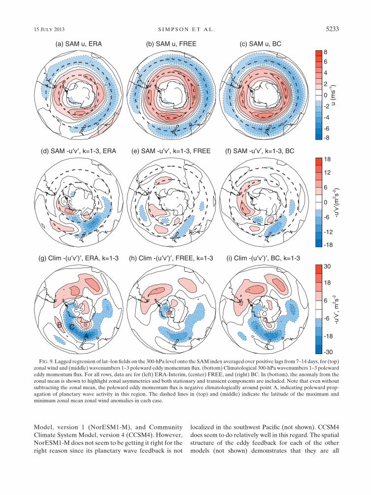
Further insight can be gained by examination of the

latitude–longitude structure of this momentum flux feed-

back. In Fig. 9 the zonal wind and k 5 1–3 momentum

flux anomalies on the 300-hPa level regressed onto the

SAM index and averaged over positive lags of 7–14 days

are shown. For ERA-Interim (Figs. 9a,d), this reveals

that accompanying a fairly zonally symmetric poleward

shift in the jet is a very zonally localized planetary wave

poleward momentum flux anomaly. In particular, the de-

creased poleward u0y0 seen in the zonal mean in Fig. 8b

is localized to the western South Pacific, southwest of

New Zealand. In FREE and BC, a localized momentum

flux anomaly occurs in the same region but it is much

weaker than the reanalysis, although slightly larger in

BC compared to FREE. Therefore, it appears that, in

order to understand the eddy feedback bias in CMAM

that is contributing to the SAM time scale bias, it will be

necessary to understand this localized planetary wave

feedback to the southwest of New Zealand and deter-

mine why it is deficient in the model.

6. CMIP5 analysis

Having identified this deficiency in planetary wave

feedbacks in CMAM it is important to determine whether

the same deficiency is exhibited by other models. The

CMIP5 archive allows this question to be addressed.

Here, the eddy feedback strengths are quantified for

theDJF season in the historical simulation for 20models

(those for which 6-hourly u and y were available at the

time of writing).

The feedback strengths are calculated for the period

1950–2005 using the methods outlined in section 3 and

the appendix. However, for CMIP5, the 6-hourly data

are only available on three pressure levels: 850, 500, and

250 hPa. The pressure-weighted vertical average over

the depth of the troposphere is performed from the cli-

matological surface pressure to 100 hPa using only these

three levels (i.e., a much coarser resolution than used in

the previous sections). There may be some quantitative

differences between results obtained using only these

three levels and those obtained with a higher vertical

resolution, but our aim here is to compare the models

with the reanalysis and CMAM and so this can be ach-

ieved by treating each model and the reanalysis in the

same way. Therefore, in the following, the CMAM and

ERA-Interim analysis has been redone using only these

three vertical levels.

The eddy feedback strengths are compared with the

SAM time scale that is obtained here using the daily

mean zonal mean zonal wind for each model. The method

of time scale calculation is the same as that used in Part I

and other studies (e.g., Gerber et al. 2010) but daily

mean zonal wind rather than geopotential height is used

as it is available for more models. The autocorrelation

function of the principal component time series PC(t) of

the first EOF of vertically averaged (using the 850-, 500-,

and 250-hPa levels) zonal wind is obtained as a function

of day of the year and lag. This is then smoothed over

a 181-day window using a Gaussian filter with a full

width at half maximum of around 42 days (standard

deviation s5 18 days). The e-folding time scale t of this

smoothed autocorrelation function is then calculated

using a least squares fit to an exponential up to a lag of

50 days. The average time scale over the DJF season is

then obtained.

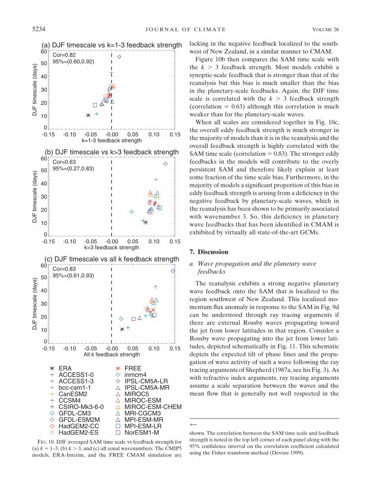
Figure 10 shows the DJF time scale versus eddy feed-

back strength divided into (a) k 5 1–3, (b) k . 3, and

(c) all k for each of the CMIP5 models. ERA-Interim

and the FREE CMAM simulation are also shown for

comparison. A first point to note is that comparison of

the ERA-Interim and FREE feedback strengths with

those in Fig. 5g shows some minor quantitative differ-

ences associated with the coarser vertical resolution

used, particularly for the synoptic scales, but these are

small and the same conclusions can be drawn as with the

full vertical resolution.

Figure 10a shows that all models exhibit a planetary-

scale feedback that is too weak compared to ERA-

Interim. The majority of the models are clustered just on

the negative side of zero, much likeCMAM. Furthermore,

the DJF SAM time scale is highly correlated with the

strength of the planetary wave feedback (correlation50.82). A fewmodels do appear to do better at exhibiting

this negative planetary wave feedback, in particular

the intermediate resolution Norwegian Earth System


Model, version 1 (NorESM1-M), and Community

Climate System Model, version 4 (CCSM4). However,

NorESM1-M does not seem to be getting it right for the

right reason since its planetary wave feedback is not

localized in the southwest Pacific (not shown). CCSM4

does seem to do relatively well in this regard. The spatial

structure of the eddy feedback for each of the other

models (not shown) demonstrates that they are all

FIG. 9. Lagged regression of lat–lon fields on the 300-hPa level onto the SAM index averaged over positive lags from 7–14 days, for (top)

zonal wind and (middle) wavenumbers 1–3 poleward eddymomentum flux. (bottom) Climatological 300-hPa wavenumbers 1–3 poleward

eddy momentum flux. For all rows, data are for (left) ERA-Interim, (center) FREE, and (right) BC. In (bottom), the anomaly from the

zonal mean is shown to highlight zonal asymmetries and both stationary and transient components are included. Note that even without

subtracting the zonal mean, the poleward eddy momentum flux is negative climatologically around point A, indicating poleward prop-

agation of planetary wave activity in this region. The dashed lines in (top) and (middle) indicate the latitude of the maximum and

minimum zonal mean zonal wind anomalies in each case.


lacking in the negative feedback localized to the south-

west of New Zealand, in a similar manner to CMAM.

Figure 10b then compares the SAM time scale with

the k . 3 feedback strength. Most models exhibit a

synoptic-scale feedback that is stronger than that of the

reanalysis but this bias is much smaller than the bias

in the planetary-scale feedbacks. Again, the DJF time

scale is correlated with the k . 3 feedback strength

(correlation 5 0.63) although this correlation is much

weaker than for the planetary-scale waves.

When all scales are considered together in Fig. 10c,

the overall eddy feedback strength is much stronger in

the majority of models than it is in the reanalysis and the

overall feedback strength is highly correlated with the

SAM time scale (correlation5 0.83). The stronger eddy

feedbacks in the models will contribute to the overly

persistent SAM and therefore likely explain at least

some fraction of the time scale bias. Furthermore, in the

majority of models a significant proportion of this bias in

eddy feedback strength is arising from a deficiency in the

negative feedback by planetary-scale waves, which in

the reanalysis has been shown to be primarily associated

with wavenumber 3. So, this deficiency in planetary

wave feedbacks that has been identified in CMAM is

exhibited by virtually all state-of-the-art GCMs.

7. Discussion

a. Wave propagation and the planetary wavefeedbacks

The reanalysis exhibits a strong negative planetary

wave feedback onto the SAM that is localized to the

region southwest of New Zealand. This localized mo-

mentum flux anomaly in response to the SAM in Fig. 9d

can be understood through ray tracing arguments if

there are external Rossby waves propagating toward

the jet from lower latitudes in that region. Consider a

Rossby wave propagating into the jet from lower lati-

tudes, depicted schematically in Fig. 11. This schematic

depicts the expected tilt of phase lines and the propa-

gation of wave activity of such a wave following the ray

tracing arguments of Shepherd (1987a, see his Fig. 3). As

with refractive index arguments, ray tracing arguments

assume a scale separation between the waves and the

mean flow that is generally not well respected in the

FIG. 10. DJF averaged SAM time scale vs feedback strength for

(a) k5 1–3, (b) k. 3, and (c) all zonal wavenumbers. The CMIP5

models, ERA-Interim, and the FREE CMAM simulation are

shown. The correlation between the SAM time scale and feedback

strength is noted in the top left corner of each panel along with the

95% confidence interval on the correlation coefficient calculated

using the Fisher transform method (Devore 1999).


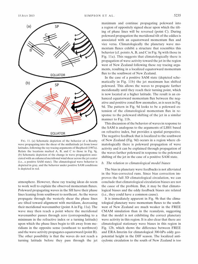
atmosphere. However, these ray tracing ideas do seem

to work well to explain the observed momentum fluxes.

Poleward propagating waves in the SH have their phase

lines leaning from southwest to northeast. As the waves

propagate through the westerly shear the phase lines

are tilted toward alignment with meridians, decreasing

their meridional wavenumber (point A in Fig. 11a). The

wave may then reach a point where the meridional

wavenumber passes through zero (corresponding to a

minimum in the refractive index or a turning latitude)

upon which the phase lines begin to tilt away from me-

ridians in the opposite sense (southeast to northwest)

and the wave activity propagates equatorward (point B).

The other possibility is that the waves do not reach a

turning latitude before they pass through the jet

maximum and continue propagating poleward into

a region of oppositely signed shear upon which the tilt-

ing of phase lines will be reversed (point C). During

poleward propagation the meridional tilt of the eddies is

associated with an equatorward momentum flux and

vice versa. Climatologically the planetary wave mo-

mentum fluxes exhibit a structure that resembles this

behavior (cf. points A, B, and C in Fig. 9g with those in

Fig. 11a). This suggests that climatologically there is

propagation of wave activity toward the jet in the region

west of New Zealand following these ray tracing argu-

ments, resulting in a localized equatorward momentum

flux to the southwest of New Zealand.

In the case of a positive SAM state (depicted sche-

matically in Fig. 11b) the jet maximum has shifted

poleward. This allows the waves to propagate farther

meridionally until they reach their turning point, which

is now located at a higher latitude. The result is an en-

hanced equatorward momentum flux between the neg-

ative and positive zonal flow anomalies, as is seen in Fig.

9d. The pattern in Fig. 9d looks to be a poleward ex-

tension of the climatological momentum flux in re-

sponse to the poleward shifting of the jet in a similar

manner to Fig. 11b.

This discussion of the behavior of waves in response to

the SAM is analogous to the arguments of LH01 based

on refractive index, but provides a spatial perspective.

The negative feedback that is localized to the southwest

of New Zealand (Fig. 9d) occurs in a region where cli-

matologically there is poleward propagation of wave

activity and it can be explained through propagation of

the waves farther poleward in response to the poleward

shifting of the jet in the case of a positive SAM state.

b. The relation to climatological model biases

The bias in planetary wave feedbacks is not alleviated

in the bias-corrected runs. Since bias correction im-

proves the full 3D climatological circulation, we can

conclude that climatological circulation biases are not

the cause of the problem. But, it may be that climato-

logical biases and the eddy feedback biases are related

(i.e., they could have a common cause).

It is immediately apparent in Fig. 9h that the clima-

tological planetary wave momentum fluxes to the south-

west of New Zealand are much weaker in the FREE

CMAM simulation than in the reanalysis, suggesting

that the model is not exhibiting the correct planetary

wave activity in this region. It is also clear that there are

climatological stationary wave biases in this region in

Fig. 12b, which shows the difference between FREE

and ERA-Interim for climatological 300-hPa eddy geo-

potential height in the DJF season. The localized anti-

cyclonic circulation to the south of New Zealand is too

FIG. 11. (a) Schematic depiction of the behavior of a Rossby

wave propagating into the shear of the midlatitude jet from lower

latitudes, following the ray tracing arguments of Shepherd (1987a).

Relate the locations marked A, B, and C to those in Fig. 9g.

(b) Schematic depiction of the change in wave propagation asso-

ciatedwith an enhancedmeridional wind shear across the jet center

(i.e., a positive SAM state). The climatological wave behavior is

depicted in gray, and the behavior under positive SAM conditions

is depicted in red.


FIG. 12. DJF climatological 300-hPa geopotential height (anomaly from the zonal mean) for (a)

ERA-Interim, (b) FREE 2 ERA-Interim, (c) BC 2 ERA-Interim, (d) the CMIP5 multimodel

mean 2 ERA-Interim, and (e) the consensus among the CMIP5 models on the sign of the geo-

potential height bias relative to ERA-Interim. The white regions in (e) indicate where less than

85%of themodels agree on the sign, blue indicates wheremore than 85%agree on a negative bias,

and red indicates where more than 85% agree on a positive bias.


weak in CMAM. Furthermore, the CMIP5 multimodel

mean exhibits a bias in this region that is strikingly

similar to CMAM (Fig. 12d), and indeed all the CMIP5

models exhibit an anticyclonic circulation that is too

weak to the south of New Zealand (Fig. 12e). How-

ever, both the climatological wave field (Fig. 12c) and

the climatological momentum flux (Fig. 9i) are sub-

stantially improved in this region by the bias correc-

tion in CMAM.

If the feedback bias is related to these climatological

biases, then the explanation must account for the fact

that bias correcting the climatology does not improve

the feedbacks. One possibility is that transience is some-

how important. Bias correction improves the climatolog-

ical wave field but it does not necessarily mean that the

transient waves that sum up to that climatology are

improved. Indeed, less than 30% of the planetary wave

feedback in ERA-Interim is associated with the sta-

tionary wave component and it can be seen in Fig. 9i

that, while the climatological circulation has been im-

proved in BC, there is still some bias in u0y0. This is nottoo surprising since climatologically u0y0 consists of bothstationary and transient components and bias correction

does not guarantee an improvement in the transient com-

ponent. For example, one possibility is that the models

are not representing the generation of transient plane-

tary waves from the tropical western Pacific correctly.

Such waves, as they follow great circle paths, would reach

the midlatitudes in this region to the southwest of New

Zealand. The study of Ding et al. (2012) has identified

wave structures in this region in the reanalysis that ap-

pear to be related to tropical processes and so the tropics

is one location in which to search for an underlying cause

of biases in planetary wave structures and feedbacks in

this region.

Another possibility is that the discussion above on the

altered propagation of planetary waves in response to

the SAM is incomplete and that, as well as changing the

eddy propagation, the SAM alters the source of Rossby

waves. For example, the climatological biases in Fig. 12

may be indicative of some deficiency in Rossby wave

generation around the New Zealand region. The SAM

may alter the generation of Rossby waves in this region

in the real atmosphere but, in the models, if this gener-

ation process is deficient then this will not happen, even

in the case where we artificially improve the climatology

by bias correction.

c. Comparison of the seasonal cycle in eddyfeedbacks with previous studies

Aside from improving our understanding of the cause

of the SAM time scale bias in CMAM, this analysis has

also provided insights into certain aspects of the

dynamics of SAM variability in the observed atmo-

sphere. Figure 7 has revealed a seasonality in the

strength of the zonal mean eddy feedbacks on the SAM

in the reanalysis with the strength of the feedback being

much reduced in the summer season from around De-

cember to March. This can be attributed to an en-

hancement of the negative feedback by planetary waves

(in particular planetary wave 3) in the summer season,

which largely offsets the positive feedback from synop-

tic-scale eddies. In a recent study, Barnes and Hartmann

(2010) examined the dynamics of SAM variability in the

summer and winter seasons. Rather than using a zonal

mean framework, they examined the 3D vorticity bud-

get and demonstrated that the winter SAM is much less

zonally symmetric: the eddy-driven jet is weak in the

Pacific sector and the circulation is dominated by the

subtropical jet there. Consequently the dominant mode

of variability in the Pacific in winter was found to be

a pulsing of the jet, rather than a latitudinal shifting.

They demonstrated that this pulsing does not invoke the

same eddy feedbacks as a latitudinal shifting does.

Based on this, they hypothesized that the SAM is more

persistent in the summer season than in the winter be-

cause in the summer the overall eddy feedbacks are

stronger (i.e., the opposite of what is found here). Their

reasoning was that in the summer the SAM represents

a zonally symmetric latitudinal shifting of the jet that

invokes a positive eddy feedback, whereas in the winter

the latitudinal shifting and the positive eddy feedbacks

are localized to the Indian Ocean sector.

Here, we find that if the eddy feedbacks on the zonal

mean SAM as a whole are considered, the total eddy

feedback on SAM zonal mean zonal wind anomalies

is actually stronger in the winter than in the summer.

Rather than being due to differences in the dynamics of

the SAM between the seasons, the present work sug-

gests that the SAM is more persistent in the SH summer

than the winter because of the presence of stratospheric

variability that occurs in the late spring/early summer

and acts to force persistent SAM anomalies in the early

part of the summer season. This influence of strato-

spheric variability is confirmed by the difference be-

tween our nudged and free-running simulations (see

Part I). That is not to say that the SAM dynamics

identified by Barnes and Hartmann (2010) are not an

important aspect of its seasonal variation, but rather we

propose that it is not the governing factor when con-

sidering the SAM time scales.

The reason for this discrepancy requires further in-

vestigation since the use of different diagnostics makes

a direct comparison between the two studies diffi-

cult. However, we can propose a couple of possibilities.

First, Barnes and Hartmann (2010) presented lagged


correlations to infer feedback strength and in the ap-

pendix we demonstrate that this may not be sufficient

to infer differences in feedback strength between sea-

sons where the intraseasonal forcing of the SAM may

differ. Second, and perhapsmore importantly, Barnes and

Hartmann (2010) focused on the upper troposphere (a

mass weighted layer between 150 and 300 hPa). The

planetary wave feedback identified here, in Fig. 8b, has

a large barotropic component. If only the upper tro-

posphere is considered, the planetary wave feedback

would appear relatively less important when com-

pared with the positive synoptic-scale eddy feedback

that is more localized to the upper troposphere. Fur-

thermore, in the transient picture, it would be expected

that eddy forcing in the middle/lower troposphere

would induce a circulation anomaly above as the at-

mosphere adjusts. It is possible that the planetary wave

forcing observed here in the vertical integral is actually

showing up in the stretching term in the upper tropo-

sphere in Barnes and Hartmann (2010). There is some

suggestion that this is the case in their Fig. 4a where a

relatively large negative forcing of the SAM by the

stretching term can be seen that is quite localized to

the southwest of New Zealand—that is, the region

where the planetary wave feedbacks identified in the

present study are strongest.

8. Conclusions

The enhanced persistence of SAM variability in the

summer season in GCMs relative to observations is a

common problem. The comparison of eddy feedbacks

on the SAM between the reanalysis and the CMAM

experiments and the CMIP5 multimodel ensemble re-

veals a commonmodel bias in the feedback by planetary

waves, in particular zonal wavenumber 3, onto the SAM

in the summertime. In the SH summer season, in the

reanalysis, the planetary waves provide a strong nega-

tive feedback onto the SAM in a localized region to the

southwest of New Zealand. The models do not seem

to capture this correctly, which likely accounts for the

greater persistence of the simulated SAM in the sum-

mertime when compared with observations.

The fact that the time scale bias can be related to a

deficiency in eddy feedbacks on the SAM is of concern

for our ability to predict future changes in the SH since

this bias in eddy feedbacks on the SAM will also likely

act on SAM-like zonal wind anomalies produced by

climate forcings such as ozone depletion or increased

greenhouse gas concentrations. All else being equal, one

might expect the models to produce SAM-like anoma-

lies in response to forcings that are too large in the DJF

season. But, GCMs [including CMAM; see McLandress

et al. (2011)] have managed to simulate trends in the

recent past in the SH midlatitude circulation reasonably

well (Son et al. 2010). This bias in eddy feedbacks then

raises this question: Are the models able to simulate

recent trends for the correct reason?

However, the main outstanding question arising from

this study is this: Why do the models not capture the

planetary wave feedbacks in the SH summer correctly?

The answer to this question will also have to explain

the seasonality in planetary wave feedbacks and its

biases. There are common biases among the models in

the climatological circulation in the southwest Pacific

in the summer season that are likely related to the

eddy feedback problem, but the CMAM bias-corrected

runs suggest that they are not the underlying cause of

it. Those simulations demonstrate that a model can

have the correctly climatology but still have the wrong

eddy feedbacks, suggesting that getting the climatology

correct for the correct reasonsmay be the key.We can put

forward a couple of hypotheses; for instance, the models

may not correctly capture the forcing of transient plane-

tary waves from the tropics correctly or may not correctly

simulate the generation of planetary waves in the vicinity

of New Zealand. Work is ongoing to investigate each of

these possibilities. Overall, the results suggest that an

improvement in our understanding of the planetary

wave feedback on the SAM and the reasons for its de-

ficiency in GCMs is necessary to improve the fidelity of

simulated SH midlatitude variability and change.

Acknowledgments. This work was funded by the

Natural Sciences and Engineering Research Council of

Canada, Environment Canada and a Lamont-Doherty

Earth Observatory postdoc fellowship. Computing re-

sources were provided by Environment Canada. We

are grateful to Michael Sigmond for making his data

for the BC simulation available, Slava Kharin for pro-

viding technical assistance in the setup of the bias cor-

rection, and Haibo Liu for aid in downloading/storage

of CMIP5 data. We also thank John Fyfe, Charles

McLandress, Richard Seager, and Bel-Helen Burgess

for helpful comments/discussion and Walt Robinson,

Dennis Hartmann, Ed Gerber, and an anonymous re-

viewer for helpful reviews.

We acknowledge the World Climate Research

Programme’s Working Group on Coupled Modelling,

which is responsible for CMIP, and we thank the climate

modeling groups for producing and making available

their model output. For CMIP the U.S. Department of

Energy’s Program for Climate Model Diagnosis and In-

tercomparison provides coordinating support and led de-

velopment of software infrastructure in partnership with

theGlobalOrganization for Earth SystemScience Portals.


APPENDIX

The Feedback Calculation and Its Uncertainties

The method used here to calculate the feedback

strength differs from that used in other studies (Lorenz

andHartmann 2001, 2003). We are motivated to use this

different method by the fact that forcing on intra-

seasonal time scales can have an important influence on

the SAM. The presence of intraseasonal forcing differs

substantially between the seasons resulting from, for

example, the presence of stratospheric variability in the

SH spring (Simpson et al. 2011) and ENSO variability

in the SH summer (L’Heureux and Thompson 2006). It

also differs substantially between the model simulations

with and without stratospheric variability. In the pres-

ence of intraseasonal forcing, the assumptions used in

the method outlined in Lorenz and Hartmann (2001)

break down. It is therefore important in our situation,

where we are comparing seasons and simulations with

different levels of intraseasonal forcing, that this be

taken into account in the feedback strength methodol-

ogy. This will be demonstrated in the following using

a synthetically generated time series of SAM zonal wind

anomalies [u]s and eddy forcing of the SAM m.

We begin by generating a synthetic time series of the

random component of the eddy forcing of the SAM ~m

using a second-order autoregressive (AR2) noise pro-

cess according to

~mt 5 0:6 ~mt212 0:3 ~mt221 �t , (A1)

where subscript t denotes day t and � is white noise dis-

tributed uniformly between21 and11. A section of this

synthetic ~m time series is shown in Fig. A1a along with

its autocorrelation function in Fig. A1c. The coefficients

of the AR2 process were chosen to give an autocorrela-

tion function that resembles that of the atmosphere (cf.

Figs. 4 and A1c). Assuming a linear model of the feed-

back, the SAM zonal wind anomalies evolve according to

›[u]s›t

5m2F[u]s, m5 ~m1b[u]s , (A2)

where F represents a frictional drag coefficient and the

eddy forcing is divided into the random component ~m

and a feedback component that is linearly related to

the SAM zonal wind anomalies b[u]s. A synthetic time

series for [u]s and m can therefore be obtained by in-

tegrating (A2) forward in time using theAR2 time series

for ~m described above. For example, the characteris-

tics of the synthetic SAM generated with F 5 0.1 and

b 5 0.04 are shown by the solid lines in Figs. A1d–f.

These parameters were chosen to provide an auto-

correlation function of [u]s and a cross correlation

between [u]s and m that resembles that of the real at-

mosphere as demonstrated by comparison of Figs. A1d,f

with Figs. 2, 5.

Now consider a situation where there is some form

of slowly varying intraseasonal forcing acting on the

SAM denoted by S. The evolution of SAM zonal wind

anomalies is now governed by

›[u]s›t

5m2F[u]s 1 S , m5 ~m1 b[u]s . (A3)

Keeping the frictional and feedback parameters exactly

the same, we now apply a small amplitude sinusoidally

varying forcing to the SAM given by S 5 0.15 sin(2pt/

200), a section of which is shown in Fig. A1b. This is not

intended to mimic a particular forcing but simply to

demonstrate what such a relatively small amplitude but

long time scale forcing does to the SAM characteristics.

The autocorrelation of [u]s and the cross correlation

between m and [u]s in the presence of S are shown by

the dashed lines in Figs. A1d and A1f. The presence of

this relatively small-amplitude intraseasonal forcing has

substantially decreased the decay rate of the [u]s auto-

correlation function (Fig. A1d). The rate of change of

the autocorrelation function as a function of lag in

Fig. A1e demonstrates that this is primarily occurring

through a difference in the rate of decay at small lags,

leaving the autocorrelation of [u]s to be larger out at

large positive lags. This is similar to what was found in

the comparison of simulations with and without strato-

spheric variability in Fig. 2 and results from the fact that

in the presence of longer time scale forcing, the shorter

time scale SAM anomalies driven by the random eddy

forcing ~m play a relatively less important role in the

autocorrelation of [u]s.

Turning to the cross correlation betweenm and [u]s in

Fig. A1f, it can be seen that the presence of this intra-

seasonal forcing substantially increases the cross corre-

lation at positive lags. Our feedback parameter b has not

changed, but the presence of the intraseasonal forcing

results in a slower decay of [u]s and as a result the cross

correlation between [u]s and m (which depends linearly

on [u]s) necessarily is larger at positive lags. This dem-

onstrates the danger of inferring the feedback strength

from the cross correlation of m and [u]s alone, in the

presence of intraseasonal forcings. The method outlined

in Lorenz and Hartmann (2001) assumes that the SAM

zonal wind anomalies obey (A2) without any form of

externally forced SAM variability. If the eddy feedback

b were to be calculated using that method, in the case


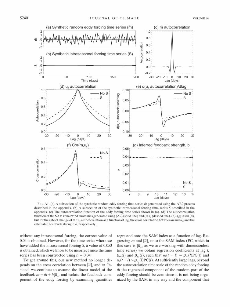
without any intraseasonal forcing, the correct value of

0.04 is obtained. However, for the time series where we

have added the intraseasonal forcing S, a value of 0.053

is obtained, whichwe know to be incorrect since the time

series has been constructed using b 5 0.04.

To get around this, our new method no longer de-

pends on the cross correlation between [u]s and m. In-

stead, we continue to assume the linear model of the

feedback m5 ~m1 b[u]s and isolate the feedback com-

ponent of the eddy forcing by examining quantities

regressed onto the SAM index as a function of lag. Re-

gressing m and [u]s onto the SAM index (PC, which in

this case is [u]s as we are working with dimensionless

time series) we obtain regression coefficients at lag l,

bm(l) and bus(l), such that m(t 1 l) ’ bm(l)PC(t) and

us(t1 l)’bus(l)PC(t). At sufficiently large lags, beyond

the autocorrelation time scale of the random eddy forcing

~m the regressed component of the random part of the

eddy forcing should be zero since it is not being orga-

nized by the SAM in any way and the component that

FIG. A1. (a) A subsection of the synthetic random eddy forcing time series ~m generated using the AR2 process

described in the appendix. (b) A subsection of the synthetic intraseasonal forcing time series S described in the

appendix. (c) The autocorrelation function of the eddy forcing time series shown in (a). (d) The autocorrelation

function of the SAMzonal wind anomalies generated using (A2) (solid line) and (A3) (dashed line). (e)–(g)As in (d),

but for the rate of change of the us autocorrelation as a function of lag, the cross correlation betweenm and us, and the

calculated feedback strength b, respectively.


shows up in them regression is solely the eddy feedback

component [i.e., bus(t1 l)’ bm(l)PC(t)]. Therefore, we

have bus(t1 l)’ bm(l)PC(t) and us(t1 l)’bus(l)PC(t).

The feedback strength can therefore be obtained by

b5bm

bus

. (A4)

This ratio is shown for both synthetic time series in

Fig. A1g between lags of17 and114 days and it can be

seen that for both time series, the feedback estimate is

b’ 0.04, as desired.The 95% confidence intervals on the

feedback strength were obtained using a bootstrapping

with replacement resampling technique. When con-

sidering a season of length nd days with ny years of

simulation/reanalysis, there are n 5 nd 3 ny days of

PC(t). To obtain an uncertainty estimate on b, PC(t) is

resampled randomly with replacement from the sample

of length n to obtain a new time series of PC of length n.

The corresponding [u]s andm data at lag l from the new

PC points are used to obtain regression coefficients bus(l)

and bm(l) for this new time series. This was done 1000

times to obtain 1000 estimates of bus(l) and bm(l). The

minimum and maximum estimates of these regression

coefficients at 95% confidence were then obtained from

this bootstrapping sample and the minimum and maxi-

mum estimates of b that these gave are taken to be the

95% confidence interval on b.

REFERENCES

Arakelian, A., and F. Codron, 2012: Southern Hemisphere jet

variability in the IPSLGCM at varying resolutions. J. Climate,

69, 3788–3799.

Baldwin, M. P., D. B. Stephenson, D. W. J. Thompson, T. J.

Dunkerton, A. J. Charlton, and A. O’Neill, 2003: Strato-

sphericmemory and skill of extended-rangeweather forecasts.

Science, 301, 636–640, doi:10.1126/science.1087143.

——, ——, and I. T. Jolliffe, 2009: Spatial weighting and iterative

projection methods for EOFs. J. Climate, 22, 234–243.

Barnes, E. A., and D. L. Hartmann, 2010: Dynamical feedbacks of

the southern annular mode in winter and summer. J. Atmos.

Sci., 67, 2320–2330.

——, ——, D. M. W. Frierson, and J. Kidston, 2010: Effect of lat-

itude on the persistence of eddy-driven jets. Geophys. Res.

Lett., 37, L11804, doi:10.1029/2010GL043199.

Dee, D. P., and Coauthors, 2011: The ERA-Interim reanalysis:

Configuration and performance of the data assimilation system.

Quart. J. Roy. Meteor. Soc., 137, 553–597, doi:10.1002/qj.828.

Devore, J. L., 1999: Probability and Statistics for Engineering and

the Sciences. 5th ed. Brooks/Cole, 535–536.

Ding, Q., E. L. Steig, D. S. Battisti, and J. M. Wallace, 2012: In-

fluence of the tropics on the southern annular mode. J. Cli-

mate, 25, 6330–6348.

Feldstein, S., and S. Lee, 1998: Is the atmospheric zonal index

driven by an eddy feedback? J. Atmos. Sci., 55, 3077–3086.Gerber, E. P., L. M. Polvani, and D. Ancukiewicz, 2008: Annular

mode time scales in the Intergovernmental Panel on Climate

Change Fourth Assessment Report models. Geophys. Res.

Lett., 35, L22707, doi:10.1029/2008GL035712.

——, and Coauthors, 2010: Stratosphere–troposphere coupling

and annular mode variability in chemistry–climate models.

J. Geophys. Res., 115, D00M06, doi:10.1029/2009JD013770.

Kidson, J. W., 1988: Indices of the Southern Hemisphere zonal

wind. J. Climate, 1, 183–194.

Kidston, J., and E. P. Gerber, 2010: Intermodel variability of the

poleward shift of the austral jet stream in the CMIP3 in-

tegrations linked to biases in 20th century climatology. Geo-

phys. Res. Lett., 37, L09708, doi:10.1029/2010GL042873.

——, D. M. W. Frierson, J. A. Renwick, and G. J. Vallis, 2010:

Observations, simulations, and dynamics of jet stream vari-

ability and annular modes. J. Climate, 23, 6186–6199.

Kuroda, Y., and H. Mukougawa, 2011: Role of medium-scale

waves on the southern annular mode. J. Geophys. Res., 116,

D22107, doi:10.1029/2011JD016293.

Leith, C. E., 1975: Climate response and fluctuation dissipation.

J. Atmos. Sci., 32, 2022–2026.

L’Heureux, L. M., and D. W. J. Thompson, 2006: Observed re-

lationships between the El Ni~no–Southern Oscillation and the

extratropical zonal-mean circulation. J. Climate, 19, 276–287.

Lorenz, D. J., andD. L. Hartmann, 2001: Eddy–zonal flow feedback

in the Southern Hemisphere. J. Atmos. Sci., 58, 3312–3327.

——, and ——, 2003: Eddy–zonal flow feedback in the Northern

Hemisphere winter. J. Climate, 16, 1212–1227.

McLandress, C., T. G. Shepherd, J. F. Scinocca, D. A. Plummer,

M. Sigmond, A. I. Jonsson, and M. C. Reader, 2011: Sepa-

rating the dynamical effects of climate change and ozone de-

pletion. Part II: SouthernHemisphere troposphere. J. Climate,

24, 1850–1868.

Robinson,W.A., 1991: The dynamics of the zonal index in a simple

model of the atmosphere. Tellus, 43A, 295–305.

——, 1996: Does eddy feedback sustain variability in the zonal

index? J. Atmos. Sci., 53, 3556–3569.

——, 2000: A baroclinic mechanism for the eddy feedback on the

zonal index. J. Atmos. Sci., 57, 415–422.Scinocca, J. F., N. A.McFarlane,M. Lazare, J. Li, andD. Plummer,

2008: Technical note: The CCCma third generation AGCM

and its extension into the middle atmosphere. Atmos. Chem.

Phys., 8, 7055–7074.

Shepherd, T. G., 1987a: Rossby waves and two-dimensional tur-

bulence in a large-scale zonal jet. J. FluidMech., 183, 467–509.——, 1987b: A spectral view of nonlinear fluxes and stationary-

transient interaction in the atmosphere. J. Atmos. Sci., 44,

1168–1178.

Simpson, I. R., P. Hitchcock, T. G. Shepherd, and J. F. Scinocca,

2011: Stratospheric variability and tropospheric annular mode

timescales. Geophys. Res. Lett., 38, L20806, doi:10.1029/

2011GL049304.

——, M. Blackburn, and J. D. Haigh, 2012: A mechanism for the

effect of tropospheric jet structure on the annular mode–like

response to stratospheric forcing. J. Atmos. Sci., 69, 2152–2170.

——, P. Hitchcock, T. G. Shepherd, and J. F. Scinocca, 2013:

Southern annular mode dynamics in observations and models.

Part I: The influence of climatological zonal wind biases in a

comprehensive GCM. J. Climate, 26, 3953–3967.

Son, S., and Coauthors, 2010: The impact of stratospheric ozone on the

Southern Hemisphere circulation changes: A multimodel assess-

ment. J. Geophys. Res., 115,D00M07, doi:10.1029/2010JD014271.

Thompson,D.W. J., and J.M.Wallace, 2000:Annularmodes in the

extratropical circulation. Part I: Month-to-month variability.

J. Climate, 13, 1000–1016.


Documents

Southern Annular Mode Dynamics in Observations and Models ... · Southern Annular Mode Dynamics in Observations and Models. Part II: Eddy Feedbacks ISLA R. SIMPSON Department of Physics,