Sources of Time Variation in the CovarianceMatrix of Interest Rates∗

Christophe Pérignon Christophe Villa

This draft: August 15, 2003

∗Christophe Pérignon is Assistant Professor at Simon Fraser University, Canada, andChristophe Villa is Assistant Professor at ENSAI (Ecole Nationale de la Statistique et del’Analyse de l’Information), CREST - LSM and CREREG - University of Rennes 1, France.We are indebted to Richard Roll for his support and helpful suggestions. We also thankMichael Brennan, Eric de Bodt, Thomas Gilbert, Amit Goyal, Rob Grauer, Bing Han,Peter Klein, Francis Longstaff, Eric Matzner-Lober, Monika Piazzesi, Michael Rockinger,Daniel Smith, Walter Torous, an anonymous referee, seminar participants at ENSAI, ES-SEC and CREREG, and participants at the Econometric Society 2003 European Meeting,Inquire UK - Inquire Europe 2003 Joint Seminar, FMA 2003 European Meeting, and AFFI2003 International Conference for their comments. This draft has been prepared for theNFA 2003 Meeting. A preliminary version of this paper was entitled ”Permanent FactorsAffecting the Dynamics of the Term Structure of Interest Rates”. Part of this research hasbeen done while Pérignon was Postdoctoral Fellow at the Anderson School at UCLA. He isgrateful for financial support from the Swiss National Science Foundation and thanks theAnderson School and UCLA for their hospitality. Emails: christophe_perignon@sfu.ca;villa@ensai.fr.

1

Sources of Time Variation in the CovarianceMatrix of Interest Rates

Abstract

In this paper, we develop a formal testing procedure, based on an innova-

tive decomposition of the covariance matrix of interest rates, to identify the

sources of time variation in the covariance among interest rates. We empir-

ically show that common factors driving U.S. interest rates display a clear

time-varying volatility. This conclusion remains valid whether or not we in-

clude in the sample the most volatile episodes in the U.S. monetary history

or when we consider recent periods. Furthermore, we conclude that loadings

on the common factors exhibit a consistent pattern across time. We report

strong empirical support for the constant factor loading assumption when

considering recent time periods and when controlling for events of extreme

volatility.

Keywords. Term Structure of Interest Rates; Time-Varying Covariance;

Principal Component Analysis

JEL Classification Codes: C13, C49, G13

2

Introduction

To the extent that economic and political conditions do change over time,

one would expect the volatility of interest rates to change as well. Indeed,

changes in business cycle conditions and monetary policy may affect real

rates and expected inflation and cause interest rates to behave quite differ-

ently in various time periods. For instance, a large number of papers (see

among others Ang and Bekaert, 2002 and Smith, 2002) have found several

episodes of large fluctuations in the volatility of the U.S. short-term interest

rates such as the 1979-1982 period, corresponding to the monetary experi-

ment, and the oil price shock in 1974. Moreover, over different time periods,

the term structure of the volatility of interest rates, the so-called volatility-

curve, looks different. Indeed, while recently the volatility-curve appears to

be hump-shaped, Dai and Singleton (2003) show that it was less humped

over the 1954-1978 period and Piazzesi (2003) attests that the hump disap-

peared during the monetary experiment. Moreover, besides volatilities, one

would except that the whole covariance matrix of interest rates to change as

well. Indeed, time variation in the covariance matrix may arise from several

sources, i.e., changing volatilities and/or changing correlations (see among

others Christiansen, 2000). In the present paper, we introduce an alternative

suitable decomposition of the covariance matrix of interest rates.

The covariance matrix of bond yield changes is often used as an input for prin-

cipal component analysis where the loadings (eigenvectors) and the volatility

(eigenvalue) of the common factors are jointly estimated (see Litterman and

Scheinkman, 1991). Empirical analysis generally determines that three fac-

tors, called the level, slope, and curvature, explain most of the movements in

interest rates. These labels have turned out to be extremely useful in think-

ing about the driving forces of the yield curve since the latent factors implied

by estimated affine models typically behave like principal components (see

Piazzesi, 2003). Such a decomposition allows one to disentangle the sources

3

of time variation in the covariance matrix of interest rates which is crucial for

managing interest-rate risk exposure and pricing interest-rate derivatives.1

Without any testing procedure, several authors have studied the evolution

through time of this decomposition of the covariance matrix of interest rates.

For instance, Bliss (1997) breaks down his 1970-1995 sample period into three

subperiods and notices that the factor loadings exhibit a consistent pattern

across the different subperiods (see also Chapman and Pearson, 2001). How-

ever, Phoa (2001) reports evidence that results on the curvature may be less

robust than those on the level and slope. On the other hand, there is evi-

dence of increased volatility of the factors during particular periods, such as

restrictive monetary policy ones (see among others Bliss, 1997 and Piazzesi,

2003). While the above studies are mainly exploratory in nature, the goal

of the current paper is to propose appropriate tests to formally identify the

sources of time variation in the covariance of interest rates.

The first step in comparing two or more covariance matrices is creating a

metric or statistic by which the comparison can be evaluated. A solution

based on maximum likelihood methods has been known for some time for

the case of covariance matrix equality (see Anderson, 1958). Basically, in

this case, each separate covariance matrix is compared to the average of all

the covariance matrices. The more different each covariance matrix is from

the average, the less likely it is that the covariance matrices are equal to

one another. In this paper, we expand on this approach by adding other

levels of similarity to the comparison, although the overall approach remains

the same. This approach is based on the Common Principal Component

1Principal component analysis is used in risk management for immunization strategies(Barber and Copper, 1996), durations (Litterman and Scheinkman, 1991), Value-at-Riskcomputations (Singh, 1997), and reduction in dimension for scenario simulation (Jamshid-ian and Zhu, 1996). This technique is also useful to price and hedge caps and swap-tions (Driessen, Klaassen and Melenberg, 2002 and Longstaff, Santa-Clara and Schwartz,2001a), or to quantify the cost of using a mispecified term structure model to price Amer-ican swaptions (Longstaff, Santa-Clara and Schwartz, 2001b).

4

(CPC) analysis and its offspring, the partial CPC analyses, which extend

the classical principal component analysis in the case of several populations

(see Flury, 1984, 1987, 1988). For each hypothesis (matrix equality, CPC,

etc), a new set of matrices is constructed by maximum likelihood methods,

and is constrained so that the hypothesis in question is true. The likelihood

that a particular hypothesis is true is determined by the relative degree of

difference between the original and constrained matrices. The difference

between the likelihood function values is distributed as a chi-square and

therefore a standard χ2 test is used to detect significant differences in matrix

structure.

Moreover, since each hypothesis may be considered as a particular model of

the term structure of interest rates, we complement the classical likelihood

ratio study by using a model building approach based on alternative infor-

mation criteria. Following this second approach, we will be able to identify

the overall best fitting model, i.e., the one with the smallest value of the

information criterion.

We apply our methodology to the U.S. term structure of interest rates over

the period January 1960 - December 1999. By initially running separate prin-

cipal component analyses in four successive subperiods, we observe that the

factor loadings remain fairly constant across subperiods whereas the volatil-

ity of the factors fluctuates substantially through time. Based on our for-

mal testing procedure, several conclusions can be drawn. We unsurprisingly

show that the assumption of a constant covariance matrix is systematically

rejected for U.S. interest rates over the last four decades. We also show that

common factors driving interest rates display a clear time-varying volatility.

This conclusion remains valid whether or not we include in the sample the

most volatile episodes in the U.S. monetary history, such as the first oil price

shock, the 1979-1982 monetary experiment, and the 1987 October stock mar-

ket crash, or when we consider more recent periods, such as the Greenspan

5

era. Furthermore, we conclude that loadings on the common factors exhibit

a consistent pattern across time. We report strong empirical support for

the constant factor loading assumption when considering recent time periods

and when controlling for events of extreme volatility. Our findings are consis-

tent with the stylized facts of U.S. term structure data and strongly support

multi-factor models allowing for time-variation in the covariance matrix of

bond yields.

The remainder of the paper is organized as follows. Section I describes the

estimation, testing, and model selection procedures. Section II presents an

empirical analysis based on the U.S. term structure of interest rates over the

last four decades. Section III concludes the paper.

6

I Understanding Similarities among Time-VaryingCovariance Matrices of Bond Yields

A The General Framework

The approach taken in this paper is to break down the covariance matrix of

bond yields at any point in time through principal component analysis. The

term structure is defined as Xt = (X1t, X2t, ..., XMt)0, whereM is the number

of maturities, and its associated covariance matrix is denoted Σt, t = 1, ..., T .

We consider three cases of interest:

• First, Σt may be assumed constant and equal to Σ for all t. In this

case, both the eigenvectors and eigenvalues are required to be constant

through time:

Σ = AΛA0 (1)

where Λ = diag(λ1, ..., λM). The jth column of A gives the eigenvectors

associated with the jth factor, and the diagonal elements of Λ give the

eigenvalues, i.e., the variances of the factors.

• Second, Σt may have constant eigenvectors but time-varying eigenval-

ues. This idea is formally expressed by the assumption that there exists

a constant orthogonal matrix A of dimension M ×M which jointly di-

agonalizes all covariance matrices Σt:

Σt = AΛtA0 (2)

where Λt = diag(λ1t, ..., λMt). In the case of several groups of data,

Flury (1984) calls this assumption the Common Principal Component

(CPC) analysis.

7

• Finally, we may assume that all the eigenvectors and eigenvalues aretime-varying. In this last case, covariance matrices at different points

in time are assumed to be totally unrelated.

Graphically, the difference between the above assumptions can easily be pre-

sented in a two-dimensional example. Consider two subperiods and two vari-

ables, x1 and x2, in each subperiod. Panel A in Figure 1 shows the two axes

or principal components, z1 and z2, obtained from a standard principal com-

ponent analysis run in each subperiod separately. We observe that the first

principal components are not the same in the two subperiods and then, by

orthogonality, the second components differ too. This situation corresponds

to the third assumption above. In each graph, the ellipse indicates the vari-

ability - the eigenvalue - associated with each principal component. Panel B

in Figure 1 presents the two principal components estimated by running a

joint analysis in both subperiods. We observe that, by construction, the two

axes are the same in both subperiods but, according to the ellipse shapes,

the variability of each principal component appears not to be the same. This

case conforms with the second assumption above. Note that if the variabil-

ity of each principal component were equal, i.e., if the ellipse shapes were

identical, then the first case would be encountered.

< insert Figure 1 >

According to factor analysis theory, three sources of time variation may be

considered for covariance matrices: the factor loadings, the factor variances,

and the residual covariance. When a covariance matrix of bond yield inno-

vations is broken down through principal component analysis, the first two

sources are overwhelmingly dominant. Indeed, Piazzesi (2003, Table 1, p.

45) shows that for the postwar period, the first three principal components

already capture over 96% of the total variation in U.S. bond yield changes.

8

In the case of bond yield levels, the proportion is even higher (over 99.5%).

Consequently, the residual covariance is a minor source of time variation in

the covariance matrix of interest rates. In this particular case, factor analysis

and principal component analysis lead to very similar results. In the follow-

ing, we therefore only consider factor loadings and factor variances, and focus

our attention on their temporal properties.

B MaximumLikelihood Estimation and Likelihood Ra-tio Tests

B.1 Maximum Likelihood Estimation

Suppose that the whole time period is divided into N consecutive subpe-

riods of size l1, ..., lN of multivariate observations X, with covariance ma-

trix Σn in the nth subperiod. Each random vector is now denoted Xn =

(X1n,X2n, ...,XMn)0, with mean zero. When Xn is a sample from the M-

variate normal distribution, Xn ∼ N(0,Σn), the joint log-likelihood function

of Σ1,..., ΣN given the sample covariance matrices S1,..., SN is given by:

lnL(Σ1, ...,ΣN) = C − 12

NXn=1

ln[ln (detΣn) + tr(Σ−1n Sn)] (3)

where C is a constant term and tr denotes the trace operator (see Anderson,

1958). The maximum likelihood estimate of Σ under:

HEquality : Σn = Σ for all n = 1, ..., N

is given by theM ×M pooled sample covariance matrix, S = l−1PN

n=1 lnSn,

where l is the total number of observations in the N subperiods.

A CPC analysis assumes that the sources of variation are constant through

time, but their magnitude may differ across subperiods. This is formally

expressed by the assumption that there exists a unique orthogonal matrix A,

which jointly diagonalizes the N covariance matrices Σn:

HCPC : A0ΣnA = Λn, n = 1, ..., N (4)

9

where A is the M ×M matrix of the eigenvectors and Λn is the diagonal

matrix of eigenvalues (λ1n, ..., λMn) in the nth subperiod.

Here, the challenge is to estimate the A and Λn matrices from the sample

covariance matrices Sn, n = 1, ..., N . If we assume that the CPC framework

is valid, Σn can be written as AΛnA0, and the joint log-likelihood function

given in Eq. (3) can be rewritten as:

lnL(Σ1, ...,ΣN) = C − 12

NXn=1

ln[ln det (AΛnA0) + tr((AΛnA

0)−1Sn)]. (5)

Flury (1984) shows that the maximum likelihood estimate of Eq. (4) can be

obtained by minimizing the following expression with respect to A:

NXn=1

ln[ln detdiag (A0SnA)− ln det (A0SnA)]. (6)

This equation is precisely a measure of the global deviation from diagonality

of the matrices A0SnA thanks to the Hadamard inequality. This inequality

states that for any positive definite symmetric matrixH, one has detH ≥ detdiag(H), with equality if and only if H is diagonal.2 Minimizing this function

can be viewed as trying to find a matrix A, which diagonalizes jointly the

matrices Sn, n = 1, ..., N, ”as much as it can”. A numerical algorithm can

be found in Flury (1988, Appendix C).

B.2 Likelihood Ratio Tests

The main advantage of the normality assumption is that likelihood-ratio tests

can be derived. For instance, Anderson (1958) shows that a test of the null

hypothesis:

HEquality : Σn = Σ for all n = 1, ..., N

2The fact that Eq. (6) can be obtained equivalently either by maximum likelihoodestimation or directly using the Hadamard inequality, which is by definition distribution-free, serves as a justification for applying the normal maximum likelihood estimation ofCPCs to nonnormal data.

10

against the general alternative one:

HUnrelated : at least one Σn differs from the others

can be conducted using a likelihood ratio-test. The statistic for testing the

hypothesis of equality versus the hypothesis of unrelated covariance matrices

is:

TEquality versus Unrelated = −2 ln L(S, ..., S)

L(S1, ..., SN)

= l ln detS −NXn=1

ln ln detSn (7)

where L(S1, ..., SN), respectively L(S, ..., S), is the unrestricted, respectively

restricted to matrix equality, maximum of the likelihood function. The sta-

tistic is asymptotically χ2 with (N−1)(M(M−1)/2+M) degrees of freedom.

A CPC analysis relies on the assumption that the matrix of eigenvectors

is constant, while the eigenvalues are allowed to vary. In this case, two

likelihood-ratio tests can be derived:3

• The first test examines whether the eigenvectors are constant throughtime. Such a test can be achieved by contrasting the CPC hypothesis

(HCPC ) with the unrelated covariance matrice hypothesis (HUnrelated ) as

follows:

TCPC versus Unrelated =NXn=1

ln ln det Σ̂n −NXn=1

ln ln detSn. (8)

Since the number of parameters estimated in a CPC analysis isM(M−1)/2 for the orthogonal matrix A, plus NM for the eigenvalues Λn, and

the number of parameters in the unrelated case is given by NM(M −1)/2+NM , then the statistic is asymptotically χ2 with (N−1)M(M−1)/2 degrees of freedom.

3We thank the referee for having suggested these two tests.

11

• The second test studies whether the eigenvalues are constant throughtime. Such a test can be achieved by contrasting the equality hypothesis

(HEquality ) with the CPC hypothesis (HCPC ) as follows:

TEquality versus CPC = TEquality versus Unrelated − TCPC versus Unrelated

= l ln detS −NXn=1

ln ln det Σ̂n (9)

where S is the pooled sample covariance matrix and Σ̂n is the covariance

matrix when the CPC hypothesis is assumed to be true. Since the

number of parameters estimated in a CPC analysis is M(M − 1)/2for the orthogonal matrix A, plus NM for the eigenvalues Λn, and the

number of parameters in the equality case is given by M(M − 1)/2 +M , then the statistic is asymptotically χ2 with (N − 1)M degrees of

freedom.

C Model Building Approach

In this section, we turn to consider each assumption given in Section I-A as

a particular model of the term structure of interest rates among which the

best model will be found. The constant covariance assumption is directly

related to the traditional principal component model. The second assumption

corresponds to the CPC model and the unrelated covariance assumption

matches the period-by-period principal component model.

We have shown that likelihood ratio tests can be constructed to discriminate

among the candidate models. However, it is well known that the chi-square

test is not always a very accurate fit index in practice since it is affected

by both the sample and model size. Indeed, larger samples produce larger

chi-squares that are more likely to be significant (type I error) and small sam-

ples may be too likely to accept poor models (type II error). Moreover, more

complicated models with many parameters tend to have larger chi-squares.

12

Instead of successively testing for the fit, or lack of fit, of each model, the

overall best fitting model should be chosen. As models with more parameters

tend to fit better out of necessity, the best model in this scheme is chosen

using a ”penalized log-likelihood”, which is a simple difference between the

log-likelihood and the number of parameters. The best model can be eval-

uated using an appropriate information criterion. The Akaike Information

Criterion (AIC) balances the goodness of fit of a particular model against

the number of parameters used to fit the model and is defined as:

AIC = −2 (maximum of log-likelihood) + 2 (number of parameters) .

Alternatively, the best fitting model can be evaluated using a Bayesian Infor-

mation Criterion (BIC), such as the one proposed by Schwarz (1978). The

BIC controls for the sample size and gives a more severe complexity penalty

than the AIC. The BIC is defined as:

BIC = −2 (maximum of log-likelihood) + ln (l) (number of parameters)

where l denotes the total number of observations in the N subperiods. For

each information criterion, the model with the lowest value is the best fitting

one.

D Generalization of the Covariance Matrix Decompo-sition

A straightforward generalization of our covariance matrix decomposition can

be proposed. Indeed, the CPC assumption can be partially relaxed by as-

suming that the Σt have some constant eigenvectors while allowing others

to be time-varying. This assumption allows a subset of m (< M) factors to

have constant loadings and a subset of M −m factors to have time-varying

loadings. This can formally be expressed by the hypothesis that the matrix

A is partitioned into eigenvectors which are constant and others that are

13

time-varying:

HpCPC : Σt = AmΛmt (A

m)0 +AM−mt ΛM−m

t

¡AM−mt

¢0(10)

where Am, of dimension M ×m, denotes the constant eigenvectors with Λmt

containing the associated eigenvalues, and AM−mt , of dimensionM×(M−m),

denotes the time-varying eigenvectors with ΛM−mt containing the associated

eigenvalues. Flury (1987) calls these assumptions the partial Common Prin-

cipal Component (pCPC) analysis.

Establishing the maximum likelihood function essentially follows the same

lines as for the CPC assumption, aside from respecting additional orthog-

onality constraints for the time-varying eigenvectors. The same system of

equations as in the CPC analysis is obtained, but a more intricate second

equation links constant and time-varying eigenvectors, making a solution la-

borious to find. Luckily, an approximate solution is available, which is based

on the insight that them common components are estimated accurately by an

ordinary CPC analysis (see Flury, 1987, Lemma 1).4 In this case, likelihood

ratio tests can be straightforwardly constructed following the same approach

as before and the associated information criteria directly computed.

4(Flury, 1987, Lemma 1): Assume that the positive definite symmetric matrices Σn ofdimension (M ×M) have m (< M) common characteristic vectors. Let these be denotedby a1, ..., am. Then the orthogonal matrix A of dimension (M ×M) that minimizes theexpression given in Eq. (6), has a1, ..., am as columns.

14

II Empirical Analysis

A Data and Preliminary Results

We now apply the methodology presented in the previous section to the U.S.

term structure of interest rates over the last four decades. The data used in

this empirical analysis are the zero-coupon bond yields from January 1960

to December 1999. According to the NBER, this sample period contains

six major recessions and six major expansions.5 Several major historical and

economic events occurred during our period of analysis (e.g. the Vietnam

war, the oil price shocks, the monetary experiment, the 1987 crash, the Gulf

war), among which some strongly impacted U.S. interest rates. The bond

yields are from the Fama Treasury Bill Term Structure CRSP file (1, 2, 3,

4, 5, 6 months) and the Fama-Bliss Discount Bonds CRSP file (1, 2, 3, 4, 5

years). The eleven bond yield time-series are continuously compounded and

available with a monthly frequency.6

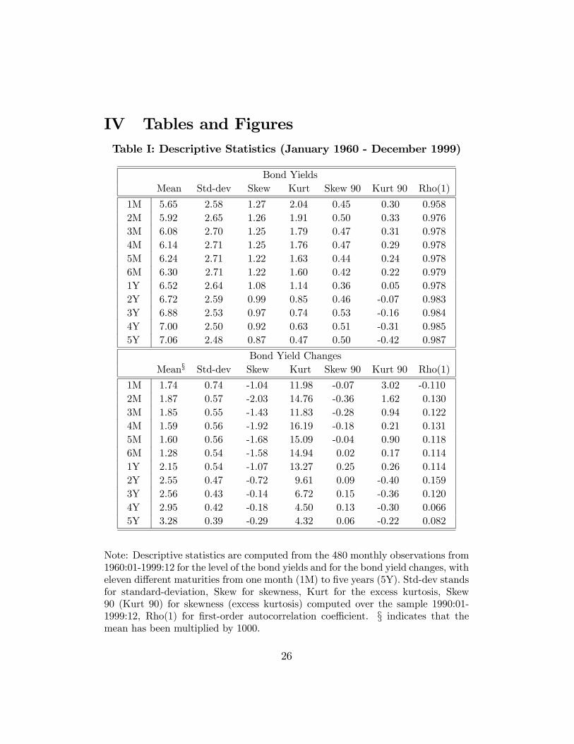
We report in Table 1 that, over the last four decades, the bond yields in-

crease on average with the maturity: the term structure is upward sloping.

The volatility of bond yield is globally decreasing with a hump at 5-6 months.

Bond yields are highly autocorrelated (around 0.980), and their distribution

appears to be slightly leptokurtic. On the other hand, bond yield changes

are far less persistent (around 0.100), but their distribution appears to be

more leptokurtic. Although the excess kurtosis does not affect the estimates

of (partial) CPCs, time dependence affects both the estimation and the test-

ing procedure.7 Furthermore, in the most recent decade, the excess kurtosis

decreases and the bond yield changes become almost Gaussian. For all these

5The NBER peaks are 1960, 1969, 1973, 1980, 1981, 1990, and 2001, and the NBERtroughs are 1961, 1970, 1975, 1980, 1982, and 1991.

6This database is a refinement of the one used by Fama and Bliss (1987), and is con-tinuously updated by the Center for Research in Security Prices (CRSP).

7We thank Michael Rockinger for pointing out the significant effect of strong temporaldependence on our testing procedure.

15

reasons, we use the demeaned bond yield changes in the following empirical

analysis.

< insert Table 1 >

In order to get a feel for the time evolution of the volatility of interest rates,

we report in Figure 2 the volatility of bond yield changes for different sample

periods. This illustrates the fact that the volatility curve may look really

different in successive time periods. Additionally, we run the Jennrich test

for the intertemporal stability of the correlation matrices by considering an

extensive number of partitions of the original sample. The values of the

statistics indicate that the assumption of stability of the correlation matrix

is systematically rejected at the 1% significance level, and this, regardless of

the compared time periods.8 We then conclude that both the variance and

the correlation of interest rate changes are definitely time-varying.

< insert Figure 2 >

As a first exploratory attempt, we run four separate principal component

analyses using 10-year non-overlapping subperiods covering respectively the

sixties, the seventies, the eighties, and the nineties. We observe in Figure

3 that the eigenvalues fluctuate substantially through time whereas the fac-

tor loadings do not seem to change appreciably across subperiods. In order

to get additional insight into the factor loading properties, we run a sim-

ple experiment with the following idea in mind: if the factor loadings were

constant through time then their estimation should not be affected by any

given partition of the total sample. To this end, we run several CPC analyses

by considering different sample breakdowns, i.e., two, three, four, and eight

8Detailed statistics on these tests are available from the authors upon request.

16

subperiods. Figure 4 shows that the estimated factor loadings on the first

three CPCs are not substantially affected by the number of subperiods con-

sidered. This last argument provides preliminary support for the constant

factor loading assumption.

< insert Figures 3 and 4>

Figure 5 plots the values of the standard-deviations of the first three fac-

tors, computed using a 12-month moving window. The value of each factor

is obtained by computing a linear combination of the original time series

of bond yield changes, where the weights are given by the factor loadings

obtained from a single principal component analysis run over the 1960-1999

sample period. We note that time-varying volatility is really about three

episodes: the oil price shock in 1974, the 1979-1982 monetary experiment,

and the 1987 stock market crash. The monetary experiment corresponds to

the period during which the Federal Reserve focused primarily on reducing

the rate of growth of monetary aggregates, rather than targeting interest

rates, in an effort to reduce inflation. We then partition our total sample

into three subperiods in order to embrace the monetary experiment and run

a separate principal component analysis in each subperiod (see Figure 6).

The first period is from January 1960 through September 1979, the second

one from October 1979 through October 1982, and the third one from No-

vember 1982 through December 1999. In Figure 6, what stands out is the

consistent pattern of the factor loadings and the really high variability of the

eigenvalues.

< insert Figures 5 and 6>

Piazzesi (2003) recognizes that any volatility study therefore has to decide

first on how to treat such volatile episodes. In order to control for the most

17

highly volatile events, we divide the total sample into four subperiods and

successively exclude the year 1974, the monetary experiment, and the Octo-

ber 1987 month. More precisely, the first period is from January 1960 through

December 1973, the second one from January 1975 through September 1979,

the third one from November 1982 through September 1987, and the last one

from November 1987 through December 1999. This alternative breakdown

of the sample will make possible to assess the impact on our conclusions of

the presence of episodes of extreme volatility.

B Empirical Results

B.1 Likelihood Ratio Tests

In order to disentangle the sources of time-varying covariance structure of

interest rates, we compare the following alternative assumptions, i.e., matrix

equality, CPC, pCPC(m), and matrix unrelatedness, using likelihood ratio

tests. Our tests are run successively with four subperiods of equal size (see

Panel A of Table 2), with the three subperiods suggested by the evolution of

interest rates (see Panel B of Table 2), and with respectively four, three, and

two subperiods excluding the highly volatile periods (see Panels C, D, E of

Table 2).

Based on the value of the likelihood ratio test presented in Eq. (7), we

can clearly reject the constant covariance assumption when testing it against

the unrelated covariance assumption, and this, whatever the sample parti-

tion considered (see Panels A-E of Table 2). For instance with the three

subperiods considered in Panel B, i.e., before the monetary experiment, the

monetary experiment, and after the monetary experiment, the T statistic is

equal to 1750.87 which is significant at the 1% confidence level.

The constant eigenvalue assumption is also strongly rejected when tested

against the CPC assumption (see Panel H of Table 2). Indeed, the likelihood

ratio test presented in Eq. (9) allows one to conclude that, whatever the time

18

period and the number of subperiods considered, the constant eigenvalue

assumption appears to be excessively restrictive for U.S. interest rates.

Similarly, according to the values taken by the likelihood ratio test presented

in Eq. (8), we can reject the constant factor loading assumption when testing

it against the unrelated covariance assumption (see Panels A-E of Table 2).

With the notable exception presented in Panel E, the CPC assumption can

indeed be rejected at the 1% confidence level. Note that the partial CPC

assumptions are also successively rejected using the different breakdowns

considered.

It appears from this battery of statistical tests that the two main components

of the covariance matrix, i.e., the eigenvalues and the factor loadings, seem to

be time-varying. The likelihood ratio approach allows one to conclude that

the most general assumption, and then the least parsimonious one, should be

preferred for modeling the dynamics of the covariance structure of interest

rates. In the following, we are going to see how this conclusion may be

affected when controlling for potential biases known to impact likelihood

ratio tests.

< insert Table 2 >

B.2 Model Building Approach

Following a model building approach, we now turn to analyzing the Akaike

and the Bayesian Information Criteria (AIC and BIC) associated with each

model: the traditional principal component model, the CPC model, the

partial CPC models, and finally, the period-by-period principal component

model. In order to clarify the presentation, we report in Table 2 the chosen

model according to each criterion using an asterisk.

Regardless of the time period and the number of subperiods considered, both

criteria clearly reject the constant covariance assumption. This fundamental

19

result implies that the traditional principal component model may turn out

to be inaccurate. Moreover, whatever the chosen criterion, the assumption of

a constant variance per factor is clearly rejected. Indeed, both information

criteria choose models with time-varying eigenvalues. It is important to point

out that, while unsurprisingly these results arise when exceptionally volatile

episodes are present in the sample, they remain valid when one considers the

1960-1999 period after having dropped the first oil price shock, the monetary

experiment, and the 1987 stock market crash (see Panel C of Table 2) or

when one considers more recent periods (see Panels D and E of Table 2).

This result shows that our conclusion on the time-varying pattern of the

covariance matrix and factor variances is not only due to the presence in the

sample of well-known highly volatile episodes.

Furthermore, we study the evolution through time of the factor structure

within a given chairman era, such as the Greenspan one. The justification of

this partition traces back to the fact that U.S. monetary policy regimes are

usually associated with Fed chairmen. Indeed, Piazzesi (2003) claims that

the different look of the volatility curves over different subperiods may be

explained by the varying degree of policy inertia under different Fed chair-

men. This argument may plead in favor of both constant covariance matrix

and constant factor variance within a given chairman term. We then divide

the Greenspan era into two equal subperiods: the first one covering August

1987 - October 1993, and the second one covering November 1993 - December

1999. In this case too, the constant covariance matrix and the constant factor

volatility hypotheses are clearly rejected since both the BIC and AIC choose

the CPC model (see Panel F of Table 2). Since the previous result may be

influenced by the 1987 stock market crash, we also consider the nineties only.

Let us recall that over this decade, bond yield changes are almost Gaussian

(see Table 1). In this case too, both the AIC and BIC conclude that the

CPC model appears to be the best model (see Panel G of Table 2).

20

According to the BIC, whatever the sample partition, the best fitting model

appears to be the CPC one, attesting that the factor loadings have not

changed appreciably in the successive time periods. Nevertheless, on panels

A to C, the AIC attests that the loadings on the factors may be time-varying.

Since the BIC gives a more severe complexity penalty than the AIC, the dif-

ferent conclusions highlight the fact that the number of parameters to be

estimated is much larger in the presence of time-varying factor loadings.9

According to the principle of parsimony, as long as the competing models

provide almost similar in-sample empirical performance, the simplest model

should always be chosen, i.e., the CPC model, as indicated by the BIC. Addi-

tional partitions also plead in favor of the constant factor loading assumption.

In particular, we report strong empirical support for the constant factor load-

ing assumption when considering recent time periods, i.e., the post-first oil

crisis era, and when controlling for the monetary experiment and the 1987

stock market crash (see Panels D and E of Table 2). These results tend to

show that rejection of the constant loading assumption is mainly driven by

the inclusion in the sample of a limited number of events of extreme volatility.

9For instance, with four subperiods, 264 parameters have to be estimated for the period-by-period principal component model versus 99 parameters for the CPC model.

21

III Concluding Remarks and Discussion

In this paper, we show that understanding the sources of time variation in the

covariance matrix of interest rates within the context of a principal compo-

nent analysis greatly expands the set of questions that can be addressed in the

study of the dynamics of interest rates. Using a formal testing procedure, we

show that the assumption of a constant covariance matrix is systematically

rejected for U.S. interest rates over the last four decades. We also show that

common factors driving interest rates display a clear time-varying volatility.

This conclusion remains valid whether or not we include in the sample the

most volatile episodes in the U.S. monetary history, such as the first oil price

shock, the 1979-1982 monetary experiment, and the 1987 stock market crash,

or when we consider more recent periods, such as the Greenspan era. Using

a model building approach, the CPC model has been shown to be the most

appropriate and parsimonious specification for U.S. interest rates. Specifi-

cally, we conclude that the best fitting model for interest rates is a model

with, on one hand, a time-varying variance per factor and on the other hand,

constant factor loadings.

Recent developments in interest rate forecasting and option pricing also plead

in favour of a CPC-type model. Indeed, Diebold and Li (2002) provide a new

interpretation of the Nelson and Siegel (1987) yield curve as a three-factor

model - where factors correspond to the level, slope, and curvature - and show

that allowing for time-varying factor loadings improves the in-sample fit by

only a few basis points. Moreover, they conclude that a forecasting model

with constant factor loadings not only fit well in-sample, but also provides

outperforming out-of-sample predictions at both short and long horizons.

Furthermore, Han (2002) develops a string market model for discount bonds

that incorporates both stochastic volatilities and correlations of the bond

yields. Under the assumption that, as in the CPC model, the instantaneous

covariance matrices at any time are diagonalized by the same matrix, the

22

covariance of bond yields is determined by the instantaneous variances of

the level, slope, and curvature factors. His model leads to smaller pricing

errors for swaptions and eliminate the large relative pricing errors between

swaptions and caps.

While our results suggest that factor loadings should be considered as con-

stant, and that even when the covariance matrix of interest rates is time-

varying, a practical question remains still open: Should we use a traditional

principal component analysis or a common principal component analysis to

estimate common factors? We do think that the common principal compo-

nent analysis approach has a manifest advantage over the standard principal

component analysis for the following reasons. First, a traditional princi-

pal component analysis does not estimate risk factors that are orthogonal

in each subperiod while a common principal component analysis systemati-

cally finds the most orthogonal ones by applying a real joint-diagonalization

criterion. Moreover, unlike traditional principal components, the common

principal components are maximum likelihood estimates and then can be

used to construct likelihood ratio tests. An even more relevant shortcoming

concerns the fact that applying a traditional principal component analysis

to the whole sample period is equivalent to estimating the factors from a

weighted sum of subperiod covariance matrices. However, it is well known

that pooling covariance matrices is not appropriate unless all subperiods are

assumed to have identical variability - a clearly rejected hypothesis for U.S.

interest rates. If the direction of the factors substantially differs from one

subperiod to another, the period with the highest variability will largely de-

termine the direction of the extracted components.

23

References[1] Anderson T. W., 1958, Introduction to Multivariate Analysis (Wiley,

New York).

[2] Ang A., Bekaert G., 2002, Short Rate Non-Linearities and RegimeSwitches, Journal of Economic Dynamics and Control 26, 1243-1274.

[3] Barber J., Copper M. L., 1996, Immunization using Principal Compo-nent Analysis, Journal of Portfolio Management Fall, 99-105.

[4] Bliss R. R., 1997, Movements in the Term Structure of Interest Rates,Federal Reserve Bank of Atlanta Economic Review 82, 16-33.

[5] Chapman D. A., Pearson N. D., 2001, Recent Advances in EstimatingTerm-Structure Models, Financial Analysts Journal 57, 77-95.

[6] Christiansen, C., 2000, Macroeconomic Announcement Effects on theCovariance Structure of Government Bond Returns, Journal of Empir-ical Finance 7, 479-507.

[7] Dai Q., Singleton K., 2003, Term Structure Modeling in Theory andReality, Review of Financial Studies 16, 631-678.

[8] Diebold F. X, Li C., 2002, Forecasting the Term Structure of Govern-ment Bond Yields, Working Paper, University of Pennsylvania (availableat http://www.ssc.upenn.edu/~fdiebold/papers/papers.html).

[9] Driessen J., Klaassen P., Melenberg B., 2002, The Performance of Multi-Factor Term Structure Models for Pricing and Hedging Caps and Swap-tions, forthcoming in Journal of Financial and Quantitative Analysis.

[10] Fama E. F., Bliss R. R., 1987, The Information in Long-Maturity For-ward Rates, American Economic Review 77, 680-692.

[11] Flury B., 1984, Common Principal Components in k Groups, Journalof the American Statistical Association 79, 892-898.

[12] Flury B., 1987, Two Generalizations of the Common Principal Compo-nent Model, Biometrika 74, 59-69.

[13] Flury B., 1988, Common Principal Components and Related Multivari-ate Models. Wiley, New York.

24

[14] Han B., 2002, Stochastic Volatilities and Correlations of BondYields, Working Paper, Ohio State University (available athttp://fisher.osu.edu/fin/faculty/han/workingpapers.htm).

[15] Jamshidian F., Zhu Y., 1996, Scenario Simulation: Theory and Method-ology, Finance and Stochastics 1, 43-67.

[16] Litterman R., Scheinkman J., 1991, Common Factors Affecting BondReturns, Journal of Fixed Income 1, 54-61.

[17] Longstaff F., Santa-Clara P., Schwartz E., 2001a, The Relative Valuationof Interest Rate Caps and Swaption: Theory and Empirical Evidence,Journal of Finance 56, 2067-2109.

[18] Longstaff F., Santa-Clara P., Schwartz E., 2001b, Throwing Away a Bil-lion Dollars: The Cost of Suboptimal Exercise Strategies in the Swap-tions Market, Journal of Financial Economics 62, 39-66.

[19] Nelson C. R., Siegel A. F., 1987, Parsimonious Modeling of Yield Curves,Journal of Business 60, 473-489.

[20] Phoa W., 2000, Yield Curve Risk Factors: Domestic and Global Con-texts, In: L. Borodovsky and M. Lore, Eds., The Practitioner’s Hand-book of Financial Risk Management (Butterworth-Heinemann, Woburn,Ma.).

[21] Piazzesi M., 2003, Affine Term Structure Models, Working Paper, UCLA(available at http://home.uchicago.edu/~piazzesi).

[22] Singh M. K., 1997, Value at Risk Using Principal Component Analysis,The Journal of Portfolio Management Fall, 101-112.

[23] Schwarz G., 1978, Estimating the Dimension of a Model, Annals ofStatistics 6, 461-464.

[24] Smith D. R., 2002, Markov-Switching and Stochastic Volatility DiffusionModels of Short-Term Interest Rates, Journal of Business and EconomicStatistics 20, 183-197.

25

IV Tables and FiguresTable I: Descriptive Statistics (January 1960 - December 1999)

Bond YieldsMean Std-dev Skew Kurt Skew 90 Kurt 90 Rho(1)

1M 5.65 2.58 1.27 2.04 0.45 0.30 0.9582M 5.92 2.65 1.26 1.91 0.50 0.33 0.9763M 6.08 2.70 1.25 1.79 0.47 0.31 0.9784M 6.14 2.71 1.25 1.76 0.47 0.29 0.9785M 6.24 2.71 1.22 1.63 0.44 0.24 0.9786M 6.30 2.71 1.22 1.60 0.42 0.22 0.9791Y 6.52 2.64 1.08 1.14 0.36 0.05 0.9782Y 6.72 2.59 0.99 0.85 0.46 -0.07 0.9833Y 6.88 2.53 0.97 0.74 0.53 -0.16 0.9844Y 7.00 2.50 0.92 0.63 0.51 -0.31 0.9855Y 7.06 2.48 0.87 0.47 0.50 -0.42 0.987

Bond Yield ChangesMean§ Std-dev Skew Kurt Skew 90 Kurt 90 Rho(1)

1M 1.74 0.74 -1.04 11.98 -0.07 3.02 -0.1102M 1.87 0.57 -2.03 14.76 -0.36 1.62 0.1303M 1.85 0.55 -1.43 11.83 -0.28 0.94 0.1224M 1.59 0.56 -1.92 16.19 -0.18 0.21 0.1315M 1.60 0.56 -1.68 15.09 -0.04 0.90 0.1186M 1.28 0.54 -1.58 14.94 0.02 0.17 0.1141Y 2.15 0.54 -1.07 13.27 0.25 0.26 0.1142Y 2.55 0.47 -0.72 9.61 0.09 -0.40 0.1593Y 2.56 0.43 -0.14 6.72 0.15 -0.36 0.1204Y 2.95 0.42 -0.18 4.50 0.13 -0.30 0.0665Y 3.28 0.39 -0.29 4.32 0.06 -0.22 0.082

Note: Descriptive statistics are computed from the 480 monthly observations from1960:01-1999:12 for the level of the bond yields and for the bond yield changes, witheleven different maturities from one month (1M) to five years (5Y). Std-dev standsfor standard-deviation, Skew for skewness, Kurt for the excess kurtosis, Skew90 (Kurt 90) for skewness (excess kurtosis) computed over the sample 1990:01-1999:12, Rho(1) for first-order autocorrelation coefficient. § indicates that themean has been multiplied by 1000.

26

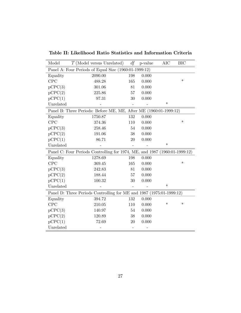
Table II: Likelihood Ratio Statistics and Information Criteria

Model T (Model versus Unrelated) df p-value AIC BIC

Panel A: Four Periods of Equal Size (1960:01-1999:12)Equality 2090.00 198 0.000CPC 488.28 165 0.000 *pCPC(3) 301.06 81 0.000pCPC(2) 225.86 57 0.000pCPC(1) 97.31 30 0.000Unrelated - - - *

Panel B: Three Periods: Before ME, ME, After ME (1960:01-1999:12)Equality 1750.87 132 0.000CPC 374.36 110 0.000 *pCPC(3) 258.46 54 0.000pCPC(2) 191.06 38 0.000pCPC(1) 86.71 20 0.000Unrelated - - - *

Panel C: Four Periods Controlling for 1974, ME, and 1987 (1960:01-1999:12)Equality 1278.69 198 0.000CPC 369.45 165 0.000 *pCPC(3) 242.83 81 0.000pCPC(2) 188.44 57 0.000pCPC(1) 100.32 30 0.000Unrelated - - - *

Panel D: Three Periods Controlling for ME and 1987 (1975:01-1999:12)Equality 394.72 132 0.000CPC 210.05 110 0.000 * *pCPC(3) 140.97 54 0.000pCPC(2) 120.89 38 0.000pCPC(1) 72.69 20 0.000Unrelated - - -

27

Table II: Likelihood Ratio Statistics and Information Criteria(continued)

Model T (Model versus Unrelated) df p-value AIC BIC

Panel E: Two Periods Controlling for 1987 (1982:11-1999:12)Equality 200.89 66 0.000CPC 75.46 55 0.035 * *pCPC(3) 43.79 27 0.022pCPC(2) 39.24 19 0.005pCPC(1) 20.05 10 0.029Unrelated - - -

Panel F: Two Periods Covering the Greenspan Era (1987:08-1999:12)Equality 183.30 66 0.000CPC 101.61 55 0.000 * *pCPC(3) 75.85 27 0.000pCPC(2) 43.25 19 0.001pCPC(1) 31.70 10 0.001Unrelated - - -

Panel G: Two Periods Covering the Nineties (1990:01-1999:12)Equality 172.09 66 0.000CPC 93.77 55 0.001 * *pCPC(3) 64.15 27 0.000pCPC(2) 54.92 19 0.000pCPC(1) 44.16 10 0.000Unrelated - - -

Panel H: Testing Equality versus CPC

Panel T (Equality versus CPC) df p-valueA 1601.72 33 0.000B 1376.51 22 0.000C 909.25 33 0.000D 184.67 22 0.000E 125.42 11 0.000F 81.69 11 0.000G 78.32 11 0.000

28

Note: In Panels A to G, alternative assumptions are tested, starting from Equalityof the covariance matrices, then common principal component (CPC), partial com-mon principal component of order three (pCPC(3)), of order two (pCPC(2)), andof order one (pCPC(1)), and ending with Unrelated covariance matrices. T (Modelversus Unrelated) denotes the likelihood ratio statistic where Model refers to, re-spectively, Equality, CPC, pCPC(3), pCPC(2), and pCPC(1). df indicates thedegree of freedom, AIC the Akaike information criterion, and BIC the Schwarzinformation criterion. * denotes the chosen model according to the AIC or BIC.ME stands for the 1979-1982 monetary experiment. The expression "controlling for1974" means that the 1974:01-1974:12 period has been removed from the sample,and similarly for the expressions "controlling for ME" and "controlling for 1987"for which the discarded periods are 1979:10-1982:10 and 1987:10, respectively. InPanel H, a likelihood ratio test contrasting the covariance equality assumptionwith the CPC assumption is presented with seven alternative sample partitions.

29

Figure Captions

Note Figure 1: In this figure, we consider two variables, x1 and x2, in two subpe-riods. Panel A shows the two axes or principal components, z1 and z2, obtainedfrom a standard principal component analysis run in each subperiod separately.We observe that the first principal components are not the same in the two subpe-riods and then, by orthogonality, the second components differ too. In each graph,the ellipse indicates the variability (the eigenvalue) associated with each principalcomponent. Panel B presents the two principal components estimated by runninga CPC analysis jointly over both subperiods. We observe that, by construction,the two axes are the same in both graphs but, according to the ellipse shapes, thevariability of each principal component appears not to be the same.

Note Figure 2: This figure presents the value of the standard-deviations of bondyield changes, for maturities ranging from 1 month to 5 years, in different timeperiods. The 1979:10-1982:10 period corresponds to the monetary experiment andthe 1987:08-1999:12 period covers the Greenspan era.

Note Figure 3: The left panels diplay the factor loadings on the first three principalcomponents in four 10-year subperiods: 1960:01-1969:12, 1970:01-1979:12, 1980:01-1989:12, and 1990:01-1999:12. The right panels display the eigenvalues of the firstthree principal components in the same four subperiods.

Note Figure 4: The panels diplay the factor loadings on the first three commonprincipal components in two 20-year subperiods, four 10-year subperiods, eight 5-year subperiods, and three unequal subperiods covering 1960:01-1979:09, 1979:10-1982:10, and 1982:11-1999:12.

Note Figure 5: This figure presents the values of the standard-deviations of thefirst three factors, computed using a 12-month moving window, over the 1961:01-1999:12 period.

Note Figure 6: The left panels diplay the factor loadings on the first three prin-cipal components in three unequal subperiods covering 1960:01-1979:09, 1979:10-1982:10, and 1982:11-1999:12. The right panels display the eigenvalues of the firstthree principal components in the three subperiods.

30

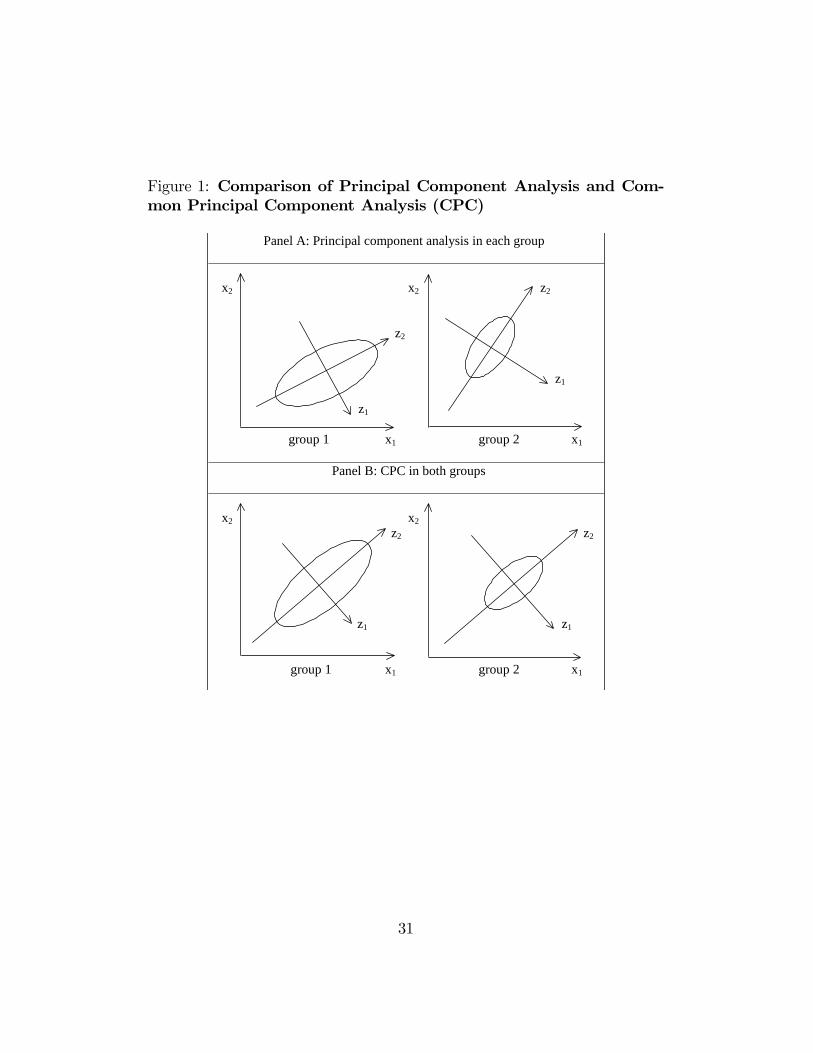
Figure 1: Comparison of Principal Component Analysis and Com-mon Principal Component Analysis (CPC)

Panel A: Principal component analysis in each group

x2 x2 z2 z2 z1 z1 group 1 x1 group 2 x1

Panel B: CPC in both groups

x2 x2

z2 z2

z1 z1 group 1 x1 group 2 x1

31

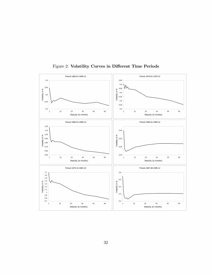
Figure 2: Volatility Curves in Different Time Periods

Period 1960:01-1969:12

0.2

0.25

0.3

0.35

0.4

1 12 23 34 45 56

Maturity (in months)

Vol

atili

ty in

%

Period 1970:01-1979:12

0.3

0.35

0.4

0.45

0.5

0.55

0.6

0.65

1 12 23 34 45 56

Maturity (in months)V

olat

ility

in %

Period 1980:01-1989:12

0.55

0.65

0.75

0.85

0.95

1.05

1.15

1.25

1 12 23 34 45 56

Maturity (in months)

Vol

atili

ty in

%

Period 1990:01-1999:12

0.15

0.25

0.35

0.45

1 12 23 34 45 56

Maturity (in months)

Vol

atili

ty in

%

Period 1979:10-1982:10

0.7

0.8

0.9

1

1.1

1.2

1.3

1.4

1.5

1.6

1.7

1 12 23 34 45 56

Maturity (in months)

Vol

atili

ty in

%

Period 1987:08-1999:12

0.2

0.3

0.4

0.5

0.6

1 12 23 34 45 56

Maturity (in months)

Vol

atili

ty in

%

32

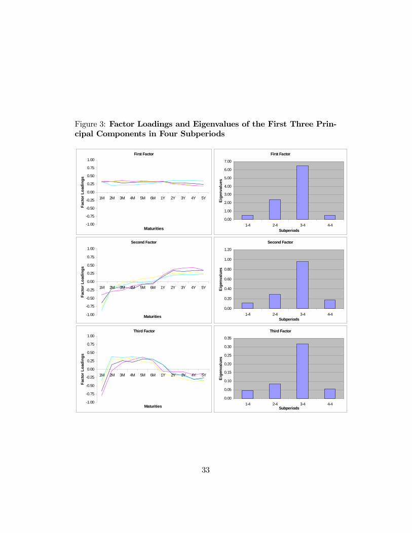
Figure 3: Factor Loadings and Eigenvalues of the First Three Prin-cipal Components in Four Subperiods

First Factor

0.00

1.00

2.00

3.00

4.00

5.00

6.00

7.00

1-4 2-4 3-4 4-4Subperiods

Eig

enva

lues

Second Factor

0.00

0.20

0.40

0.60

0.80

1.00

1.20

1-4 2-4 3-4 4-4Subperiods

Eig

enva

lues

Third Factor

0.00

0.05

0.10

0.15

0.20

0.25

0.30

0.35

1-4 2-4 3-4 4-4Subperiods

Eig

enva

lues

Second Factor

-1.00

-0.75

-0.50

-0.25

0.00

0.25

0.50

0.75

1.00

1M 2M 3M 4M 5M 6M 1Y 2Y 3Y 4Y 5Y

Maturities

Fact

or L

oadi

ngs

Third Factor

-1.00

-0.75

-0.50

-0.25

0.00

0.25

0.50

0.75

1.00

1M 2M 3M 4M 5M 6M 1Y 2Y 3Y 4Y 5Y

Maturities

Fact

or L

oadi

ngs

First Factor

-1.00

-0.75

-0.50

-0.25

0.00

0.25

0.50

0.75

1.00

1M 2M 3M 4M 5M 6M 1Y 2Y 3Y 4Y 5Y

Maturities

Fact

or L

oadi

ngs

33

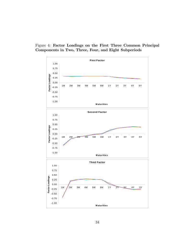
Figure 4: Factor Loadings on the First Three Common PrincipalComponents in Two, Three, Four, and Eight Subperiods

First Factor

-1.00

-0.75

-0.50

-0.25

0.00

0.25

0.50

0.75

1.00

1M 2M 3M 4M 5M 6M 1Y 2Y 3Y 4Y 5Y

M aturitie s

Fact

or L

oadi

ngs

Second Factor

-1.00

-0.75

-0.50

-0.25

0.00

0.25

0.50

0.75

1.00

1M 2M 3M 4M 5M 6M 1Y 2Y 3Y 4Y 5Y

M aturitie s

Fact

or L

oadi

ngs

Third Factor

-1.00

-0.75

-0.50

-0.25

0.00

0.25

0.50

0.75

1.00

1M 2M 3M 4M 5M 6M 1Y 2Y 3Y 4Y 5Y

M aturitie s

Fact

or L

oadi

ngs

34

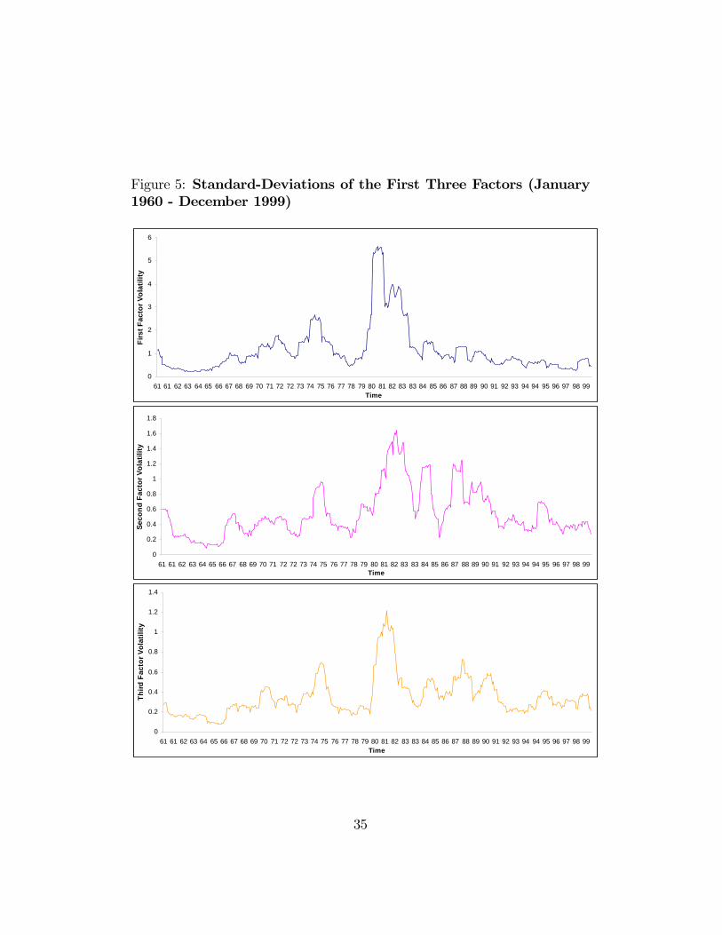
Figure 5: Standard-Deviations of the First Three Factors (January1960 - December 1999)

0

1

2

3

4

5

6

61 61 62 63 64 65 66 67 68 69 70 71 72 72 73 74 75 76 77 78 79 80 81 82 83 83 84 85 86 87 88 89 90 91 92 93 94 94 95 96 97 98 99Time

Firs

t Fac

tor V

olat

ility

0

0.2

0.4

0.6

0.8

1

1.2

1.4

1.6

1.8

61 61 62 63 64 65 66 67 68 69 70 71 72 72 73 74 75 76 77 78 79 80 81 82 83 83 84 85 86 87 88 89 90 91 92 93 94 94 95 96 97 98 99Time

Seco

nd F

acto

r Vol

atili

ty

0

0.2

0.4

0.6

0.8

1

1.2

1.4

61 61 62 63 64 65 66 67 68 69 70 71 72 72 73 74 75 76 77 78 79 80 81 82 83 83 84 85 86 87 88 89 90 91 92 93 94 94 95 96 97 98 99Time

Third

Fac

tor V

olat

ility

35

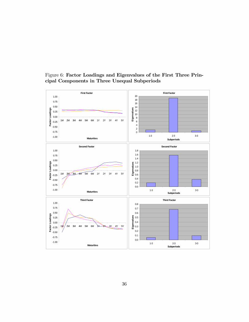
Figure 6: Factor Loadings and Eigenvalues of the First Three Prin-cipal Components in Three Unequal Subperiods

First Factor

02468

101214161820

1-3 2-3 3-3Subperiods

Eige

nval

ues

Second Factor

0.0

0.20.4

0.6

0.81.0

1.2

1.41.6

1.8

1-3 2-3 3-3Subperiods

Eige

nval

ues

Third Factor

0.0

0.1

0.2

0.3

0.4

0.5

0.6

0.7

0.8

1-3 2-3 3-3Subperiods

Eige

nval

ues

First Factor

-1.00

-0.75

-0.50

-0.25

0.00

0.25

0.50

0.75

1.00

1M 2M 3M 4M 5M 6M 1Y 2Y 3Y 4Y 5Y

Maturities

Fact

or L

oadi

ngs

Second Factor

-1.00

-0.75

-0.50

-0.25

0.00

0.25

0.50

0.75

1.00

1M 2M 3M 4M 5M 6M 1Y 2Y 3Y 4Y 5Y

Maturities

Fact

or L

oadi

ngs

Third Factor

-1.00

-0.75

-0.50

-0.25

0.00

0.25

0.50

0.75

1.00

1M 2M 3M 4M 5M 6M 1Y 2Y 3Y 4Y 5Y

Maturities

Fact

or L

oadi

ngs

36