Sources of Productivity Growth Duringthe Transition to AlternativeCropping Systems

Edward C. Jaenicke and Laurie E. Drinkwater

Traditional measures of productivity growth may not fully account for all sources of growth

during the transition from conventional to alternative cropping systems. This paper treats soil

quality as part of the production process and incorporates it directly into rotational measures

of productivity growth. An application to data from an experimental cropping system in

Pennsylvania suggests that both experimental learning and soil-qtrrdity improvements were

important sources of growth during the system’s transition.

Concern over the environmental consequences ofconventional agricultural practices has led re-searchers to develop alternative practices and crop-ping systems that are designed to be both profitableand environmentally benign. Economic compari-sons of alternative and conventional systems gen-erally show that alternative practices can be com-petitive if there is a substantial input-cost savings,an output price premium, a reduction in revenuerisk through output diversification, or an account-ing of the social costs associated with agriculturalpollution (Hanson et al.; Hanson, Lichtenberg, andPeters; Lee; Smolik, Dobbs, and Rickerl; Faeth etal.; Sahs and Lesoing; Ikerd, Monson, and VanDyke; National Research Council 1989).

Data from on-farm research suggest that thesoil-plant environment undergoes a biological tran-sition upon conversion from conventional to alter-native practices. Several analysts and practitionershave identified transitional costs associated withthe conversion period (Dabbert and Madden; Mac-Rae et al.; Bender) and other researchers have sug-gested that economic comparisons may favor con-ventional practices over alternative practices dur-ing this period (Hanson et al.; Andrews et al.;Culik; Janke et al.). Not always mentioned in thesestudies is the growth in managerial expertise andknowledge that may be required to successfullysurvive the transition period. Both types of transi-tional costs—--le,, the investment in both human

Edward C. Jaenicke is an assistant prnfessor in the Department of Ag-ricultural Econurrrics and Rural Sociology at The University of Tennes-see. Laurie Drinkwater is with the Rodale Institute in Pennsylvania.

We would like to thank Bnb Chambers and Rolf Ftie fnr commentingon earlier versions of this paper.

capital and soil capital—may present barriers tothe general adoption of alternative agriculturalpractices (Batie and Swinton; Lockeretz).

Traditional measures of productivity growthmay not completely account for all sources ofgrowth during the transition period. In particular,productivity measures may not reflect the invest-ment in soil quality. For example, just as Grilichesand later Jorgenson and Griliches showed that ob-served aggregate total-factor productivity growthcould be mistaken labor- and capital-quality im-provements, productivity growth in an alternativecropping system could be mistaken for soil-qualityimprovements. Accounting for soil-qualitychanges may be particularly important when inves-tigating alternative cropping practices, which aredesigned to increase soil quality through diversecrop rotations and green manures. Excluding thiscomponent from productivity calculations duringthe transition period may entangle growth due tolearnin with growth due to soil-quality improve-ments. F The implication is that successful eco-nomic implementation of alternative cropping sys-tems may require both soil-quality improvementsand learning by doing.

This paper treats soil quality as part of the pro-

1To see the consequences from ignoring soil-quality changes in simi-lar settings, one could turn to (i) soil productivity studies that investigatethe affect erosion has on crop productivity (Crosson; Pierce et al.; Put-nam, Williams, and Sawyev Walker and Yorrn& Xu and Prato) or (ii)recent developing country studies that have attempted to explain thenbserved inverse relationship between farm size and farm productivityby presenting evidence that smaller farms have higher land quality(Bhalkv Bhalla and Roy; Benjamin; Sampath).

170 October 1999 Agricultural and Resource Economics Review

duction process and incorporates it directly into aMalmquist-type productivity index (see Caves,Christensen, and Diewert; Fare et al.; Fare,Grosskopf, and Lovell). For example, when Fiire,Grosskopf, and Roos compute productivity growthin Swedish pharmacies, they simply incorporateservice-quality indicators (such as customer wait-ing time, promptness of service, and hours of op-eration) into the Malmquist index as separate out-puts. When no service-quality outputs are includedin their Malmquist index, productivity measure-ments from one year to the next show a 2.4?Z0im-provement. When service-quality outputs are in-cluded, however, the productivity increase drops to1.8% due to a slight deterioration, on average, ofsame-day service and average waiting time.

The same type of direct adjustment is used hereto incorporate soil quality into Malmquist produc-tivity indexes. This adjustment requires soil-testdata matched to production data, a rare combina-tion. Fortunately data from farming-system experi-ments conducted at the Rodale Institute ResearchCenter (Rodale) in Kutztown, Pennsylvania, pro-vide a unique opportunity to construct soil-quality-adjusted Malmquist indexes of on-farm productiv-ity. This opportunity is not without limitations andseveral characteristics of the data will complicatethe construction and interpretation of the Malm-quist indexes.

First, total organic matter is the only soil param-eter that Rodale has consistently measured at theplot level and, hence, it must serve as the soleindicator of soil quality. While current researchsuggests that soil quality is best characterized by abroad array of soil parameters-a so-called mini-mum data set for soil quality (Kennedy and Pap-endick; Doran and Parkin; Larson and Pierce;Karlen and Stott), several studies suggest that totalorganic matter is one of the most important singleindicators of soil quality (National Research Coun-cil 1993; Arshad and Coen; Romig et al.).

Second, it is important for productivity measuresand the underlying representation of the productiontechnology to reflect Rodale’s rotational croppingsystems. One method for modeling rotational pro-duction is to treat each sequential crop rotation asa single multi-year process that includes all theinputs and outputs over the entire multi-year rota-tion. This method, however, can lead to degrees-of-freedom problems for estimating econometricmodels of rotational production. One solution tothis empirical problem is the use of data envelop-ment analysis (DEA) methods to construct a non-parametric model of the multi-year productionprocess using mathematical programming tech-

niques.2 Strengths of DEA methods include: (i) theability to estimate models using data with insuffi-cient degrees of freedom for traditional economet-ric techniques such as ordinary least squares ormaximum likelihood estimation, (ii) the ability toovercome extreme invariability in the data, (iii) theability to calculate productivity measures basedonly on quantity data, (iv) the ability to modelproduction without imposing a functional form,and (v) the ability to accommodate inefficiency.One weakness of DEA is a susceptibility to dataoutliers (Burgess and Wilson); another is a dimen-sionality problem where a large number of inputsand outputs relative to the number of observationscan lead most or even all plots to lie on the pro-duction frontier (Leibenstein and Maital; Tauerand Hanchar). A third weakness is the general per-ception that there can be no statistical inferencebecause of the deterministic nature of DEA meth-ods (Grosskopf). Rotational crop data may lead toa dimensionality problem because of the poten-tially large number of crop inputs and outputsthroughout a rotation. Moreover, weather data maypose a particular problem for DEA methods be-cause abnormal, stochastic weather events can leadto data outliers. Fortunately, recent work byBanker (1996 and 1993) has explored the statisticalproperties of DEA estimators and can be used totest statistical hypotheses.

Third, Rodale has incorporated technologicalimprovements into its cropping systems, particu-larly in its alternative (organic) systems. This prac-tice is common to most long-term field experi-ments to keep cropping systems relevant (Steiner;Frye and Thomas). Because Rodale’s alternativesystem was not well established, however, experi-mental learning may be the biggest source for tech-nological improvements. For example, after evalu-ating early outcomes from its alternative system,Rodale switched from a short-season com varietyto the same long-season variety used in its conven-tional system. The Malmquist index results, how-ever, will not distinguish experimental learningand the improvements it has generated as separatesources of growth.

Fourth, Rodale has staggered the rotation’s entrypoint on separate fields so experimental learningpotentially may be applied across fields as well asacross rotations. The production model to followdoes not distinguish between these two applica-tions of experimental learning, but their implica-

2 Lovell provides a good introduction to productivity measurementusing DEA methods.

Jaenicke and Drinkwater Sources of Productivity Growth 171

tions will be discussed along with the Malmquistindex results.

And fifth, the Rodale data, like data from otherexperimental trials, may differ from data generatedfrom “real-world” farming situations. However,because Rodale’s systems were managed for per-formance and altered to incorporate new technolo-gies—both learned and acquired, they should moreclosely reflect the practices of real-world farmersthan more rigid agronomic trials.

With these five limitations in mind, the objec-tives of this paper are to develop a method forinvestigating the sources of growth in an alterna-tive cropping system and apply it to Rodale’s ex-perimental data to draw inferences about thesources of productivity growth. Particular empha-sis is given to the transition period, interpreted hereas ending around the alternative system’s fifthyear. Specifically, this paper attempts to: (i)present and apply a rotational model of crop pro-duction, (ii) use DEA techniques to calculate twosets of farm-level productivity measures forRodale, one that is adjusted to reflect soil-qualitychanges brought on by cropping-practice choiceand one that ignores soil-quality changes, (iii) testthe importance of including soil quality in themodel using the hypothesis tests developed byBanker (1993 and 1996), and (iv) compare the ad-justed and unadjusted measures to examine thesources of growth in Rodale’s alternative croppingsystem.

A Model of Rotational Production andProductivity Change

The model presented here, which takes theoreticaland empirical research by Chambers and Lichten-berg as a starting point, differs from traditionalproduction models in two important ways: First, itassumes that production occurs on a rotational ba-sis so that the technology set includes all time-dated inputs and outputs over the entire crop rota-tion. Second, it treats soil quality as a capital goodand includes it in the technology set. Without thesetwo important deviations from traditional models,one would be unable to attribute productivitygrowth to soil-quality improvements or the experi-mental learning that occurs after each completedcrop rotation.

Following Chambers and Lichtenberg, define acrop rotation as a recurring multiyear croppingcycle, during which a sequence of crops is pro-duced with a sequence of inputs. Let T be the num-ber of years in a complete crop rotation. Let M andN be the maximum number of outputs and inputsfor any year within a complete rotation. Let y, e

‘x+M,t= 1, ..., T, be the vector of all cropoutputs produced in year t of the T-year rotationand let Y = [y,, y2, . . . . y~] be the vector of alltime-dated outputs produced over the entire rota-tion. Similarly, let xt ● 93+~, t=l, . . .. T. be thevector of all crop inputs applied in year t of aT-year rotation and let X = [xl, x2, . . . . XT]be thevector of all time-dated inputs applied over theentire rotation.

Suppose that soil quality is measured at the endof the year (or growing season) and that the end-of-year soil-quality indicators in one year areequivalent to the beginning-of-year indicators inthe next year. Let Q equal the number of soil-quality indicators measured during each period andstE!R+Q,t= o,..., T, represent the vector of allend-of-year soil-quality indicators in year t.Thenlet S_~ = [s., . . . . s~_ll represent the vector of allthe beginning-of-year indicators over the entire T-year rotation, and let S_O= [s,, . . . . s~] representthe vector of all the end-of-year indicators over theentire rotation.

Because productivity change may occur fromone completed rotation to the next, it is necessaryto date a particular rotation and the underlying in-puts, outputs, and soil-quality indicators. There-fore, assume one can observe R temporally-sequenced, T-year rotations and can index each byre [l,..., R]. The index, r, dates each completerotation. It will sometimes be useful to index out-puts, inputs, and soil-quality variables by the rota-tion number. For example, in rotation r, Y’ = [yrl,Y’29...7 yrT], x’ = [Xrl , X’2, . . . . X’T], s_Tr=[sr~, . . . . SrT_l], and S_Or = [S’l, . . . . S“T]. Con-sider a three-crop, three-year rotation where oats,corn, and soybeans are produced in years one, two,and three. In this rotation, the vector Y = [oats~,com2, soybeans~] reflects the quantity of outputproduced in each year of the rotation. (Conceiv-ably, double cropping or intercropping could leadto more than one crop output in each year.) Each

!?re eated rotation is indexed by the superscript r: soY describes the oatslcornlsoybean output foryears one to three; Y2 describes the output foryears four to six.

For rotation number r, assume the process thattransforms all crop inputs and beginning-of-seasonsoil-quality indicators throughout the rotation intocrop outputs and end-of-season soil-quality indica-tors can be modeled by the rotational output setY’S(X, S.~), where

Y“~(X,S-T) = {(Y, S_O):(X, S_T) can produce(Y, S_O)at rotation r}.

Y’s(X, S_~) allows inputs in year t to affect cropproduction directly in subsequent years. It treats all

172 October 1999 Agricultural and Resource Economics Review

outputs over the entire cycle as joint outputs,thereby implicitly capturing all the biological,chemical, and physical soil processes throughoutthe rotation. To be useful in modeling production,output sets like Y“~(X,S_~) are assumed to satisfya number of axiomatic properties such as convex-ity, disposability, closeness, and boundedness,3

The rotational output set can be approximatedfor empirical purposes by constructing a referencetechnology, equivalent to the free-disposal, convexhull of the data, using mathematical programmingtechniques common to DEA (see Ftire, Grosskopf,and Lovell). Let K denote the number of observa-tions in each completed rotation and define the setof data as

T(K,R) = {(Yr)k, S’Ik_o, X“k, Sr’k_~): k = 1, ., , ,K,r=l, . . .. R).

For each rotation r, let the set of indexes be de-noted as

I(K,r) = {1’, . . . . K},

The approximation to the general output set, la-beled as Yr~(X, S_T), is constructed according toFare, Grosskopf, and Lovell’s general method,where

(1)

~~(xr, S!T) = {(Y’, S!j): Y’ ~ ~ Yr’kZr’k, (i)ke Z(K,r)

(iv)

Zr’kG m+, (v)

The variable Z’)k, “indexed by r and k, is an intensityvariable indicating the role each kth production ob-servation plays in determining the frontier withinrotation r. In essence, the vector Zrallows for con-vex combinations of the data. The constraints (1.i)through (1vi) require the reference technology

3 Fare and Chamhers each discuss axiomatic properties of generaloutput sets, The production technology could also be modeled with aninput set or a feasible-production set, Chambers and Lichtenberg presentother variations of the rotational production model that assume produc-tion within the rotation can be septwated in annual production processes,

Yr~~(X, S_~) to be the piecewise linear, convexFull’of the data that exhibits non-increasing returnsto scale and free disposability of inputs and out-puts. Specifically, constraints (1.i) and (1ii) im-pose free disposability on all crop outputs and soil-quality outputs throughout the entire rotation.4Constraints (1iii) and (1iv) impose free dispos-ability on all crop inputs and soil-quality inputsthroughout the entire rotation. Finally, constraint(1.vi), together with constraint (1.v), imposes non-increasing returns to scale, which allows all radialcontractions of the observed data, but not radialexpansions, to belong to the reference technology.5For the case of a single crop output and a singlesoil-quality output, the reference technology maybe depicted as all points on or inside OABCD infigure 1.

The reference technology is next used to esti-mate a distance function (Shephard), a generaliza-tion of production function that represents the larg-est feasible radial expansion of crop outputs andsoil-quality outputs. For the reference technologyspecified in (1), define the rotational output dis-tance function as

(2)D’s(Y, S.., X, S_~) = [max {0 >0: (OY, W-O)

e ~’~(x, s_~) }]-1,

For a point like E in figure 1, the value of thedistance function is given by OE/OB.All points likeE that are elements of ~~(X, S_T)have a distancefunction value of less than or equal to one; allpoints that are not elements, like F, have a distancefunction value greater than one.

The rotational model allows for a well-knownsynergistic rotation effect, where yields from cropsgrown in rotations are higher than yields fromcrops grown in isolated monoculture (Cook;Magdoffi Power; National Research Council1989). The rotational model accounts for this effectdirectly by allowing for complementary joint pro-duction throughout the entire rotation and indi-rectly by allowing soil-quality investment to returnhigher yields in later periods.

A reference technology that excludes soil qual-ity can be derived from the reference technology in

4 Chambers and L1chtenberg suggest that free output dkposabilitymay rule out some forms nf complementarily amnng outputs that couldbe essential in modeling some cropping systems, Free nutput disposabil-ity, however, is imposed here to rule out programming infeasibMies.

5 The non-increasing retrims constraint (1 ,vi), which proves useful inruling out prograrnrrdng infeasibilities, is a natural consequence if at leastone element of X is constant across all K observations. In the applicationthat follows, land area (or in this case plot size) is identical for all K, afact that transforms constraint (1.iii) into constraint ( I.vi),

Jaenicke and Drinkwater Sources of Productivity Growth 173

‘i.

)

yt

Figure 1. The Reference Technology and Dis-tance Function

(1). Let the approximation to the rotationalset that excludes soil quality be given by

(3)~_~(X7 = {W (I,i), (1.iii), (1.v),

and (1vi) hold].

output

The set Y’_~(X) says all outputs throughout theentire ro~tion are produced jointly in the sameproduction process. While it ignores contributionsfrom soil quality, this set still accounts for a rota-tion effect because it, like Y“~(X,S_T), allows forcomplementary production:

As before, the approximation can be used toestimate distance functions. Define the rotationaloutput distance function without soil quality as

(4)fY_~(Y, X) = [max {El>0: (8Y) E Yr_#i’)}]-l.

Following Fare, Grosskopf, and Lovell’smethod, define the rotational Malmquist output in-dexes—with and without soil quality—of rota-tional productivity change as6

6 The Malmquist index is directly related to other indexes of produc-tivity change. Caves, Christensen, and Diewert shuw that if the technol-

ogy Of two firms can be represented by translog distance functions (withidentical second-order coefficients), then the geometric mean of theirMalmquist indexes evaluated for the two profit-maximizing firms underconstant returns to scale is identical to the Tornqvist index of produc-tivity change, an exact and superlative index measure,

[

m+l(yN’,sg ;x’+’,Sy )(5) Ms(r,r+l) =

D: (Yr, S1.; X’, SIT) 1

and

D: (Yr, S~; X’, S&)

(6)

[

D~l (Ywl; Xtil)lk.~(r,r+l) =

DI~ (Yr; X’) 1

[ 1D[~ (Y’; X’) Dc~ (YH1; X’+l) 1’2

D[~l (Yr; X’) Dfl~l (Yfi’ ; X’+l) ‘

Productivity is progressive from one rotation toanother if (5) and (6) are greater than one, andregressive if they are less than one. F&-eet al. showthat the first bracketed term in (5) and (6) is anefficiency-change index and the second term is atechnical-change index.

Comparisons between (5) and (6) will addressthe role soil quality plays in productivity growth.In particular, Banker (1996 and 1993) suggeststhree hypothesis tests that can be used to determinewhether two technologies are statistically differ-ent.7 In essence, there are two separate questions toask of the two technologies, namely (i) are thereference technologies specified by (2) and (4) sta-tistically different, and (ii) are the productivity-,technical-, and efficiency-change index measuresspecified in (5) and (6) themselves statistically dif-ferent. Banker’s tests can be applied, in some fash-ion, to answer both questions.

Banker’s (1996) first two tests are based on theassumptions that the reciprocals of the distancefunction values (often called Farrell efficiencymeasures) follow the exponential or half-normaldistribution, Banker’s (1996) third test, a Kolmog-orov-Smirrtov test, is useful when no particular as-sumptions can be maintained about the probabilitydistribution of distance function values. The distri-bution-free test, therefore, is especially useful fordirectly comparing the Malmquist index results.Because each index calculation in (5) and (6) is afunction of four distance functions, two standarddistance functions and two intertemporal distancefunctions, it would be awkward to assume that the

7 Grosskopf discusses recent research by S,A.C. Kittelsen that pro-vides evidence of the small-sample properties of Banker’s tests.

174 October 1999 Agricultural and Resource Economics Review

Year

19831984198519861987198819891990199119921993

Field 1 Field 2 Field 3

ISmallgrains corn

corn Smallgrains ISmallgrains*

cornSoybeans

SmallgrainsCorn

SoybeansCorn

SoybeansSmallgrains

* Soil organic mattermeasurementsare unavailable for this year.

Figure 2. Rodale’s Alternative Cropping System Outputs by Year

results follow the exponential, half-normal, or anyother particular distribution.

Rodale’s Experiments and Data

In 1981, Rodale initiated its Farming Systems Tri-als, a long-term study to examine the process ofconverting from a conventional to an alternativecropping system. Because the goal of Farming Sys-tem Trials was to compare two or more systems,variation within each system was kept to a mini-mum. Rodale kept input application rates for fieldlabor and seed, among other inputs, relatively con-stant; however, it has tinkered with its alternativesystem to improve performance. Productivity mea-surements will pick up this tinkering as improve-ments in technology or efficiency due to experi-mental learning, Two potential sources of variationreflected in the data are year-to-year differences inweather, and plot-to-plot differences in the soil.

Malmquist indexes are crdculated for Rodale’salternative system, which is based on a diversecrop rotation that relies on a green manure andmechanical cultivation for the system’s fertilityand pest control, The alternative system is a three-year rotation that produces a crop of small grainslike oats or barley in the first year, a legume covercrop (like red clover) followed by com in the sec-

ond year, and a spring barley crop, if possible,followed by soybeans in the third year. The alter-native system was started at three different pointsin the rotation and replicated eight times in a split-plot, randomized complete block design (Janke etal.). Each of the replications was grown on 20 by300 foot plots. The rotation was designed as a re-curring cycle so that, in the empirical analysis, itsstarting point can be treated as arbitrary and pickedto maximize the number of usable data observa-tions.

Figure 2 summarizes the field replications forthe alternative system. Data from the replicationsare considered usable if rotational inputs and out-puts are comparable from one rotation to the next.The figure indicates that Rodale has tinkered withthe alternative system, interrupting the three-yearrotation in several places. It also indicates that, inone year, soil-quality data are unavailable for oneof the fields. Hence, there are only 16 usable ob-servations (two fields times eight replicated plots)over three complete rotations for the alternativesystem. The clear boxes in figure 2 correspond todata observations in the first (r = 1) rotation; thelight shaded boxes and the dark shaded boxes cor-respond to observations in the second (r = 2) andthird (r = 3) rotations.

The reference technologies presented above re-quire three types of data-crop yields, levels or

Jaenicke and Drinkrvater Sources of Productivity Growth 175

rates of cropping inputs (including weather inputs),and soil-quality measurements—that correspond tothe Y, X, and S vectors. Plot-level crop yields thatcomprise the Yvector were measured after harvest-ing the entire plot, excluding output from the plotborders (about 33% of the plot area), and reportedon a per-hectare basis. The actual elements of Yarelisted in figure 2 and in table 1. Inputs to the al-ternative system (elements of X) included yearlylabor, yearly rainfall, and the nitrogen equivalentfound in the green manure that precedes corn, Thesole soil-quality indicators (elements of S) avail-able were yearly measures of soil organic matter.Table 1 presents the mean values for all elementsof the Y, X, and S vectors for both cropping sys-tems. (A detailed description of the rotational datacan be found in Hanson, Lichtenberg, and Peters,or Chambers and Lichtenberg. ) In general, cornyields in the alternative system were lower thanconventional corn yields at the start, but increasedto near comparable levels by the end of the period.Soybean yields in the alternative system sufferedtowards the end of the period, possibly due to in-creased weed pressure. Soil organic matter in-creased substantially throughout the period. For themost part, average rainfall decreased in most yearsfrom one rotation to the next, The nitrogen equiva-lent of the alternative system’s green manure var-ied widely from year to year: on average, it

Table 1. Average Values for RotationalOutputs, Inputs, and Soil-Quality Measuresfor Rodale’s Alternative Svstem

).=1 f.=z r=3

YSmall grain, 2532.4Corng 8240.1Soybeans? 4160.2xLaborl 2.14Precipl 52.3Labor2 2.19N2 129.5Precip2 47.3Laborq 1.97Precips 46.0sOrg. Matter. 1.82Org. Matterl 2.26Org. Matter2 2.32Org. Matters 2.42

Units:Yields = kg/traLabor = hours/acreNitrogen equivalent (N = lbs/acre)Precipitation = inches per yearOrganic matter = %

2711,1 3580.37938.3 9005.82560.3 3051.2

1.47 1,90

46.1 42,81,69 2.11

76.0 95,042.5 42,5

1.51 1,8345.4 46.6

2.42 2,892.63 2.712.32 3.792,66 3.51

dropped from nearly 130 pounds per acre in thefirst rotation cycle to 76 and 95 pounds per acre,respectively, in the second and third cycles.

Rodale’s scientists generally estimate that thetransition period for the alternative system endedin 1985 or 1986, approximately five years after theexperiment’s 1981 start date (Andrews et al.). Ifthis is true, then productivity-growth measures thatcompare the first two completed rotations shouldreflect what happened as the alternative systemcame out of transition. Comparison between thesecond and third completed rotation should reflecta post-transition period.

Results

Table 2 presents the Malmquist productivity indexand its technical-change and efficiency-changecomponents from (5) and (6), calculated forRodale’s alternative cropping system, The tablepresents a side-by-side comparison of plot-levelindex calculations for the reference technology thataccounts for soil quality along with the corre-sponding reference technology that excludes soilquality. Notice that table 2 contains two sets ofcalculations, one indexing the shift between thefirst and second rotations, and another indexing theshift between the second and third rotations.

Plot-level index calculations represent thechange from one completed rotation to the next.For example, column 1 of table 2 shows that theproductivity change for plot number 1 of the alter-native system is 1.38600 for the rotational modelwith soil quality. In this case, one could say thatthe productivity increased 38.6% on this plot fromthe first to second rotations. At the bottom of thetable are two rows of summary statistics: the geo-metric average and the variance of the sampleplots. For example, table 2 shows that productivityincreased, on average, 14.9470when soil quality isincluded in the alternative system’s model.

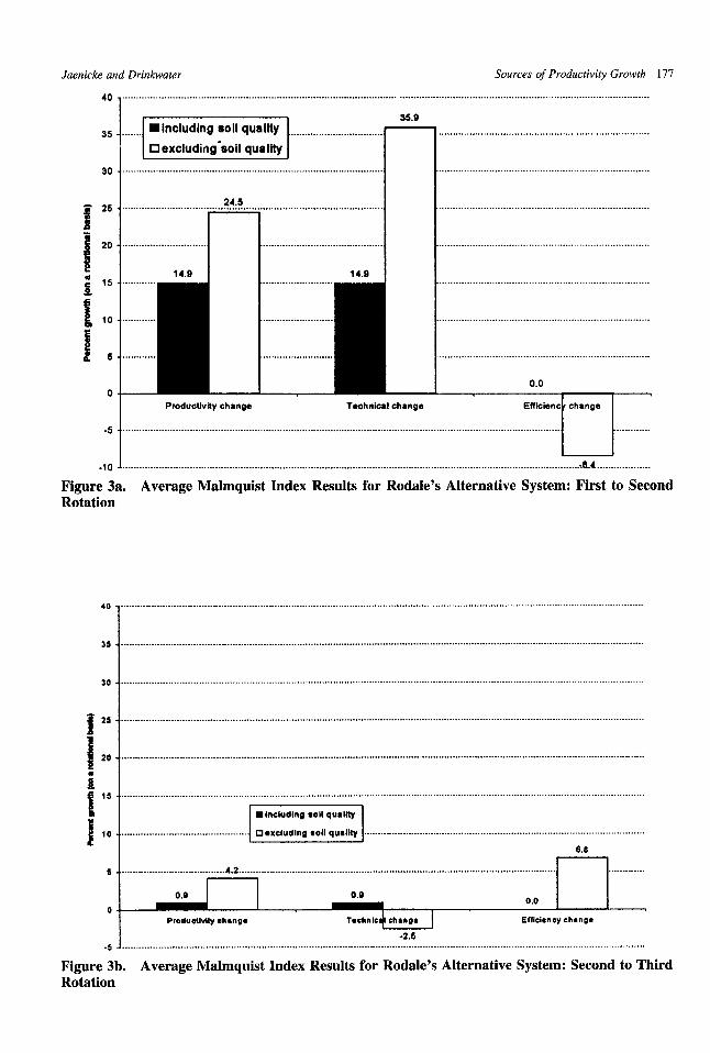
Figures 3a and 3b present graphical summariesof the average productivity-, technical-, and effi-ciency-change results for Rodale’s alternative sys-tem. For example, figure 3a shows that productiv-ity increased, on average, 14.9% from the first tosecond alternative rotation when soil quality wasincluded. However, figure 3b shows that this cal-culation dropped to 0,9% when measured from thesecond to the third rotation,

Table 3a presents the results of Banker’s threetests. Here, the null hypothesis is that within eachcompleted rotation the distance-function values(actually, the Farrell efficiency measures) have the

176 October 1999 Agricultural and Resource Economics Review

Table 2. Technical and Efficiency Change On Rodale’s Alternative System Using RotationalModels that Account for Soil Quality (S) or Exclude Soil Quality (-S)

(a) First to Second RotationProductivity Change Technicat Change Efficiency Change

Plot No. s -s s -s s -s

123456789

101112

13

141516

Gee. Avg.var.

(b) Second to Third Rotation

Plot No.

(1)1.386001,549511.287681.295461,603141,276041.261261.487220.890791,057680.954000.997481.149800.804910.842720.964901.149360.06516

(2)1.524111.707801.681841.673721.695771.488131.472851.704060.982660.983031.048320.868021.038220,965850.868690,940671,245240.12214

Productivity Change

s –s

(3) (4)1,38600 1.868051.54951 1.824371.28768 1.698211.29546 1.650221.60314 1.695771.27604 1.599361.26126 1.710451.48722 1.807600.89079 1.135761.05768 1.085530,95400 1,048320.99748 1,072311.14980 1,038220.80491 1.041330.84272 1.100920.96490 1.024411.14936 1.358980.06516 0.12202

Technical Change

s -s

(5) (6)1.0000Q 0.815881.00000 0.936101.Oootxl 0.990361.00000 1.014241.00000 1.000001.00000 0.930451.00000 0.861091.00000 0.942721.00000 0.865211.00000 0.905581.00000 1.000001.00000 0.809491.00000 1.000001.00000 0,927521.00000 0.789061.00000 0.918261.00000 0,916130,00000 0.00539

Efficiency Change

s -s

123456789

10111213

14

15

16Gee, Avg.Var.

(1)0.868670.946230.829340.834800.878120.926930.926580.828081.178201.269551.045871.343411.190431.225711,048931.006331.008800.02922

(2)0.773460.806140.812820.798850.808450.854531.023950.763741.251801.355011.056991.540491.24230

1.352281.543961.236601.042210.08033

(3)0.868670.946230.829340.834800.878120.926930.926580.828081.178201.26955

1.045871.343411.190431.225711.048931.006331.008800.02922

(4)0.783240.779330.818000.798850.808450.795100.823100.770231.178101.218801.110511.209691.242301.214641.178681.204130.975420.04306

(5)1.000001.000001.000001.000001.000001.000001.000001.000001.000001.000001.000001.000001.000001.000001.000001.000001.000000.00000

(6)0.815880.936100.990361.014241.000000.930450.861090.942720.865210.905581.000000.809491.000000.927520.789060.918260.916130.00539

same distribution, no matter whether soil qualitywas accounted for or excluded. Table 3a suggeststhat the null hypothesis can be widely rejected.Simply stated, the exponential, half-normal, andKolmogorov-Smirnov tests all show that the twomodels, one with soil quality and one without it,are statistically different. These results add weightto assertions that soil quality can be isolated as asubstantial source of growth in the alternative sys-tem.

Table 3b presents the results from Banker’s thirdtest on the productivity-, technical-, and efficiency-change calculations themselves. Formally, the Kol-

mogorov-Smirnov test is applied to the null hy-pothesis that the two distributions of index calcu-lations, one with soil quality and one without, areidentical. All but one of the individual tests inTable 3b show that there are significant differencesbetween the two types of results; a productivityindex result from the first to second rotation provesto be an exception,

The results in tables 2 and 3 and the summariesin figures 3a and 3b provide the basis for threebroad conclusions: (1) a large portion of Rodale’salternative system’s substantial growth was due tosoil-quality improvements; (2) the large productiv-

Jaenicke and Drin.kwater Sources of Productive@Growth 177

40

35

30

- 25

~

I

20

; ‘5

f!~ 10

! 5

0

-5

.10

‘“””””=■ includlng soil quality ...............................

... ..... .. . ... .. .. ......... ........ ...... ....... .......... .. .............

24.5.. ... ....... ........ .. .... ... .... ...... ...

............. ..... .. .... .. .

14.9. ... .

...... ....

.... .......

Productivity change

............. ..........................

14.9.. .. . . .. . . . .. . . . .. .. . . .. .

4

.. . . . .. . . . . . . . . . . .. .

... . . . . . . . . . . . . .. . .. . .. ..

35.9

Technical change

0.0

Effkienc TA

............. ..-.&4 . . . . . .. . . . . . . . . . .. .

Figure 3a. Average Malmquist Index Results for Rodale’s Alternative System: First to SecondRotation

40

35

30

i2s

120

i

!15

I10

5

0

-s

6.8I

Produclivlty changeu

Tochnlc chmga Efflclmcy change

...........

Figure 3b. Average Malmquist Index Results for Rodale’s Alternative System: Second to ThirdRotation

178 October 1999 Agricultural and Resource Economics Review

Table 3. Are the Rotational Models With and Without Soil Quality Statistically Different?*

(a) Results from Banker’s ~hree hypothesis tests based on the calculated value of the distance functions

Exponential Hatf-Normal Komorgorov-Test Test Smirnov Test

Fkst rotation yes yes yesSecond rotation yes yes yesThird rotation yes yes yes

(b) Results from Banker’s nonparametric Kolmorgorov-Smirnov test based on the index calculations

Productivity Change Technicat Change Efficiency Change

First to second rotation no yes yesSecond to third rotation yes~ yes yes

*One-tailed tests at the %’.SZO confidence level, unless otherwise noted.tSignificantly different using a one-tailed test at the 95% confidence level

ity-growth residual that remained after soil qualityis accounted for can be attributed to experimentallearning; and (3) these two sources of growth,learning and soil-quality improvements, were es-pecially important as the alternative systememerged from the transition period.

Soil-quality improvements

The Malmquist index calculations, on average,show that soil quality was an important source ofthe alternative system’s overall growth because,when soil quality was unaccounted for, productiv-ity growth and technical change were substantiallyoverestimated. For example, figures 3a and 3bshow that average productivity growth is overesti-mated by 9.6$Z0(24.5Y0 versus 14.9Yo) from thefirst to second rotation and by 3.3% (4.2Y0versus0.9%) from the second to the third rotation. Thefigures show the same pattern for technical change,although the technical-change measurement fromthe second to the third alternative rotation providesan exception to this pattern. To the extent that qual-ity improvements explain a large portion of pro-ductivity growth and technical change, these re-sults are reminiscent of Jorgenson and Griliches’sresults. Here the results suggest that soil qualityexplains a large part of the supposedly unexplainedproductivity-growth and technical-change residualobserved in Rodale’s alternative system, especiallyduring the first two completed rotations.

Productivity results for some individual plotscontradict the average results. For example, table 2shows productivity growth from the first to secondrotation is underestimated on four individual plotswhen soil quality is omitted; and from the secondto third rotation, productivity growth is underesti-mated on seven individual plots when soil qualityis omitted. This apparent contradiction (with indi-vidual results contradicting the average results)

provides a lesson on interpreting the results. Whenexamining productivity growth, one considers rela-tive, not absolute, growth in inputs and outputs.Because the rotational model treats soil quality asboth an input and an output, a soil quality improve-ment has implications on both soil-quality inputgrowth and soil-quality output growth. Whengrowth in the soil-quality output is greater thangrowth in the soil-quality input, one might under-state productivity growth when soil quality isomitted (even if absolute levels of soil quality areincreasing). Put another way, positive levels ofsoil-quality growth are consistent with higher pro-ductivity growth measures after accounting for soilquality.

Experimental learning

Figures 3a and 3b (along with table 2) provideevidence that substantial learning occurred in thealternative system, even after accounting for soilquality. For example, productivity in the alterna-tive system improved 14.9% over the first two ro-tations, a six-year period. Because the rotationalmodel accounts for labor, nutrients, weather, andsoil quality, these factors are unlikely to be thesource of productivity growth or technical changeunless the available data are misrepresentative.sHowever, information on at least one major factoris missing in the production model: managerial ex-pertise. Experimental learning is the likely sourceof the managerial improvements and, therefore, theproductivity-growth and technical-change residual.As mentioned above, Rodale has acted on this ex-perimental learning by tinkering with the alterna-

8 According to Rodale, monthly rainfall may better characterizeweather differences than annual rainfall, which is used in this study.Furthermore, because a single soil parameter may inadequately reflectsoil quality, soil quality may be misrepresented,

Jaenicke and DrinkWater Sources of Productivi~ Growth 179

tive system. Unfortunately, experimental learningand the tinkering it has generated cannot be distin-guished as separate sources of Rodale’s technicalprogress. In this case, the high rates of technicalprogress may be documentation of the tinkeringitself,

As mentioned in the introduction, the staggerednature of Rodale’s experimental design may fur-ther complicate the issue of experimental learning.The staggering in figure 2 suggests that learningfrom field one could be applied to field two, re-sulting in higher initial performance in field twobut lower initial productivity growth. Indeed theindexes for individual plots in table 2 reflect thepossibility of across-field learning from the first tosecond rotation: plots 1–8 (field one) have higherproductivity growth than plots 9–16 (field two).gThis scenario is reversed, however, when resultsfrom the second to third rotations are examined.Hence, across-field learning, if it is occurring, islimited to the early part of the experiment. Thereversal in field-to-field differences in productiv-ity-growth results may be explained, at least inpart, by the cyclic nature of productivity measures.For example, low productivity in rotation r canlead to negative productivity-growth measure-ments from r – 1 to r but positive measurementsfrom rto r+ l.]O

Transition period

If Rodale’s transition period lasted five years or so,then the productivity results that compare the firsttwo alternative rotations roughly demonstrate whathappened when the system emerged from the tran-sition period. Figures 3a and 3b show that produc-tivity and technical change improved substantiallyfrom the first to the second rotation but onlyslightly from the second to the third. These obser-vations are just what one would expect when theemergence occurs during the first measurement pe-riod but not the second,

Conclusion

Results show that the rotation-based productivitymeasures that ignore soil quality, on average, over-

9 Banker’s Kolmorgorov-Smimov test confirms that productivityy re-sults from plots 1-8 are significantly different than results from plots9–16. (Banker’s two parametric tests cannot he applied because a di-mensionality problem, which causes all plots to have a distaace functionvalue equal to one, necessitates division by zero. ) Thanks to aa anony-mous reviewer for suggesting both that across-field learning may explainthe results and that Banker’s test may be useful.

IO For ~omp~~on, ~ ~~e, annual productivity-growth reversals we

fairly common in Ball et al.’s total factor productivity results over asimilar 15-year period for the aggregate agricultural sector.

state productivity growth for Rodale’s alternativecropping system, which features a nitrogen-richgreen manure, Results also show that the alterna-tive system’s high initial rates of productivitygrowth drop after two complete rotations. Takentogether, these results suggest that the high growthrate observed as Rodale’s alternative systememerged from the transition period can be directlyattributed to two sources: returns on soil capitalinvestment and/or gains from experimental learn-ing.

These results are in several ways intuitive oranticipated. For example, it makes sense that pro-ductivity growth was overstated when soil qualitywas excluded because the alternative system wasdesigned to achieve high crop yields by buildingup soil capital. If the investment in soil quality wasunaccounted for, the growth in yields as the systememerged from transition would appear to be unex-plained and therefore may have been assigned totechnical progress. By comparing productivityymeasures with and without soil quality, one clearlysees that the investment in soil quality was a majorsource of growth.

It is also intuitive that the technical progress, orlearning, associated with Rodale’s alternative sys-tem would grow at a high pace, especially as thealternative system emerged from the transition pe-riod. At the start of the experiment, Rodale’s al-ternative rotation was new, untested, and unsup-ported by a fully developed network of alternativeagricultural practitioners and researchers. For ex-ample, Rodale’s experiments were already at leastfive-years old when research on alternative agri-cultural practices entered federal agriculturalpolicy (in the form of the Low-Input SustainableAgriculture research and education program,which saw authorization in the 1985 Farm Bill andappropriations in 1988). In other words, Rodalepractitioners could expect to face a steep learningcurve on their alternative system. This paper’s con-tribution is the confirmation of these expectationsby documenting the sources of growth during thetransition period through the application of re-cently proposed theoretical models and hypothesistests.

By documenting these two sources of growth,the paper also exposes an issue underlying thecritical economic question of whether alternativesystems can be economically competitive withconventional systems. The productivityy results,while not designed to evaluate economic competi-tiveness, do suggest that to be practitioners of al-ternative systems must overcome two transitionalcosts—investments in soil capital and managementcapital—to survive the transition period.

180 October 1999 Agriculwral and Resource Economics Review

References Diewert, WE. 1976. “Exact and Superlative Index Numbers.”

J. of Econometrics4:115-145.

Andrews, R.W., S.E. Peters, R.R. Janke, and W.W. Sahs. 1990.

“Converting to Sustainable Farming Systems.” In C.A.

Francis, C.B. Flora, and L.D. King, eds. WtaitzableAg-riculture in Temperate Zones. New York: John Wiley &

Sons.

Arshad, M. A., and G. M. Coen. 1992. ’<Characterization of Soil

Quality: Physical and Chemical Criteria.” Amer. J. of Al-

temative Agriculture ‘7:25-31.

Ball, V. E., J.-C. Btrreau, R. Nehring, and A. Somwam. 1997.“Agricultural Productivity Revisited.” Amer. J. Agr. Econ.

79:1045-1063.

Banker, R.D. 1996. ’’Hypothesis Tests Using Data Envelopment

Analysis.” Journal of Productivity Analysis 7:139-159.

Banker, R.D. 1993. “Maximum Likelihood, Consistency and

Data Envelopment Analysis: A Statistical Foundation.”

Management Science 39:1265-1273.

Batie, S, B., smd S.M. Swinton. 1994. “InstitutionalI ssuesand

Strategies for Sustainable Agriculture: View from Within

the Land-Grant University.” Am. J. of Ahernative Agricul-

ture9(Nos. 1 and2):23–27.

Bender, J, 1994. Future Harvest: Pesticide- free Farming. Lin-

coln, NE: Univ. of Nebraska Press.

Benjamin, D. 1995. ’’Can Unobserved Land Quality Explain the

Inverse Productivity Relationship?” Journal of Develop-

ment Economics 46:5 1–84.

Bhalla, S.S. 1988. “Does Land Quality Matter?” Journal of

Development Economics 29:45-62.

Bhalla, S. S., and P. Roy, 1988. “Mis-Specification in Famr

Productivity Analysis: The Role of Land Quality.” Oxford

Economic Papers 40:55-73.

Burgess, J. F., and P.W. Wilson. 1993. ’’Technical Efficiency in

Veterans Administration Hospitals.” In H.O. Fried, C.A.K.

Lovell, and S.S. Schmidt, eds, The Measurement of Pro-

ductive E~iciency. New York: Oxford University Press.

Caves, D. W., L. R. Christensen, and W. E. Diewert. 1982. ’’The

Economic Theory of Index Numbers and the Measurement

of Input, Output, and Productivity.” Econometrics 50:

1393–1414.

Chambers, R.G. 1988. Applied Production Analysis: A Dual

Approach. New York: Cambridge University Press.

Chambers, R. G., and E. Lichtenberg. 1995. ’’Economics of Sus-

tainable Farming in the Mid-Atlantic.” Department of Ag-

ricultural and Resource Economics, University of Mary-

land, Final Report tothe USDA/EPA ACE Program.

Cook, R.J. 1991. ’’Challenges and Rewards of Sustainable Ag-riculture Research and Education.” In Sustainable Agricul-

ture Research and Education in the Field:A Proceedings,

Board on Agriculture, National Research Council. Wash-

ington, DC: National Academy Press.

Crosson, P,R. 1983. Productivity Effects of Cropland Erosion in

the United States. Washington, DC: Resources For the

Future.

Culik, MN. 1983. “The Conversion Experiment: Reducing

Farm Costs.”J. of Soil and Water Conservation 38:333-

335.

Dabbert, S., and P. Madden. 1986. ’’The Transition to Organic

Agriculture: A Multi-year Simulation Model of a Pennsyl-

vania Farm.’’ Am. J. of Alternative Agriculture 1:99–107.

Doran, J.W., and T.B. Parkin. 1994. “Defininga ndAssessing

Soil Quality.” In J.W. Doran, D.C. Coleman, D.F.

Bezdicek, and B.A. Stewart. Madison, eds, Defining Soil

QualicY for a Sustainable Environment: SSSA Special Pub-

lication Number 35. WI: Soil Science Society of America.

Faeth, P., R. Repetto, K. Kroll, Q. Dai, and G. Helmers. 1991.

Paying the Farm Bill: US. Agricultural Policy and the

Transition to Sustainable Agriculture. Washington, D.C.:

World Resources Institute.

Fare, R. 1988. Fundamentals of Production Theory. New York:

Springer-Verlag.

Ftie, R., S. Grosskopf, B. Lindgren, and P. Roos. 1994. ’’Pro-

ductivity Developments in Swedish Hospitals: A Malm-

quist Output Index Approach.” In A. Charnes, W.W. Coo-

per, A.Y. Lewin, and L.M. Seiford, eds, Data Envelopment

Analysis: Theory, Methodology, and Applications. Boston:

Kluwer Academic Publishers.

Fare, R., S. Grosskopf, and C.A.K. Lovell. 1994. Production

Frontiers. New York: Cambridge Univ. Press.

Ftie, R., S. Grosskopf, and P. Roos. 1995. “Productivity and

Quality Changes in Swedish Pharmacies.” Int ‘1,Journal of

Production Economics 39:137-147.

Frye, W. W., and G. W. Thomas. 1991. ’’Management of Long-

Term Field Experiments.’’ Agronomy J. 83:38-44.

Griliches, Z. 1963. “The Sources of Measured Productivity

Growth: U.S. Agriculture, 1940-1960.”J. Pol. Econ. 71:

331-346.

Grosskopf, S. 1996. “Statistical Inference and Nonparametric

Efficiency. A Selective Survey.’’ Journal of Productivity

Analysis 7:161-176.

Hanson, J.C., E. Lichtenberg, and S.E. Peters. 1997. “Organic

Versus Conventional Grain Production in the Mid-

Atlantic: An Economic and Farming Systems Overview.”

Am, JoumalofAlternative Agriculture 12:2–9.

Hanson, J. C,, D. M. Johnson, S.E. Peters, and R. Janke. 1990.

“TheProfitability of Sustainable Agriculture ona Repre-

sentative Grain Famr in the Mid-Atlantic Region, 1981–

89,’’ Northeastern J. of Ag. and Res. Econ. 19:90-98.

Ikerd, J., S. Monson, and D. Van Dyke. 1993. “Alternative

Farming Systems for U.S. Agriculture New Estimates of

Profhand Environmental Effects.” Choices (Third Quar-

ter):37–38.

Janke, R. R., J. Mt. Pleasant, S.E. Peters, and M. Bohlke. 1991.

“Long-Term, Low-Input Cropping Systems Research.” In

Sustainable Agriculture Research and Education in the

Field: A Proceedings, National Research Council. Wash-

ington, D. C.: National Academy Press.

Jorgenson, D. W., and Z. Griliches. 1967. “TheExplanationofProductivity Change.’’ Rev. Econ. Srudies34:249–283.

Karlen, D. L., and D.E. Stott. 1994. “AFrameworkf orEvalu-

sting Physical and Chemical Indicators of Soil Quality.” In

J.W. Doran, DC. Coleman, D.F, Bezdicek, and B.A. Stew-

art. Madison, eds, Defining Soil Quality for a Sustainable

Environment: SSSASpecial Publication Number 35. WI:

Soil Science Society of America.

Kennedy, A. C., and R. I. Papendick. 1995. “MicrobialCharac-

teristics of Soil Quality .’’Journal of Soil and Water Con-

servation 50:243–248,

Jaenicke and Drirrkwater Sources of Productivity Growth 181

Larson, W. E., and F.J. Pierce. 1994. ‘The Dynamics of Soil

Quality as a Measure of Sustainable Management.” In J.W.

Doran, D.C. Coleman, D.F. Bezdicek, and B.A. Stewart.

Madison, eds, Defining Soil Quality for Sustainable Envi-

ronment: SSSA Special Publication Number 35. WI: Soil

Science Society of America.

Lee, L.K. 1992. “A Perspective on the Economic Impacts of

Reducing Agricultural Chemical Use.’’ Am. Jor Aherrra-

tive Agriculture 7:82–88.

Leibenstein, H,, and S. Maital. 1992. “Empirical Estimation and

Partitioning of X-Inefficiency: A Data-Envelopment Ap-

proach.” Amer. Econ. Rev. 82:428433.

Lockeretz, W. 1991. “Information Requirements of Reduced-

Chemical Production Methods.” Am. J. or Alternative Ag-

riculture 6:97–103.

Lovell, C.A.K. 1993, ’’Production Frontiers and Productive Ef-

ficiency.” In H.O. Fried, C.A.K. Lovell, and S.S. Schmidt,

eds, The Measurement of Productive Efficiency. New

York: Oxford University Press.

MacRae, R.J., S.B. Hill, J. Henning, and A.J. Bentley. 1990.

“Policies Programs, and Regulations to Support the Tran-

sition to Sustainable Agriculture in Canada.” Am. J. of

Alternative Agriculture 5(2):76-92.

Magdoff, F. 1992. Building Soils forgetter Crops: Organic

Matter Management. Lincoln, NE: Univ. of Nebraska

Press.

National Research Council. 1993. Soil and Water Quality:An

Agenda for Agriculture. Washington, D. C,: NationalAcademy Press.

National Research Council. 1989. Alternative Agriculture.

Washington, D.C.: National Academy Press.

Pierce, F.J., R.H. Dowdy, W. E. Larson, and W.A.P. Graham.

1984, “Soil Productivity in the Corn Belt: An Assessment

of Erosion’s Long-Term Effects.” Journal of Soil and Wa-

ter Conservation 39:13 1–143.

Power, J.F. “Legumes: Their Potential Role in Agricultural Pro-ductility.’’ Am. J, of Alternative Agriculture 2:69–73.

Putman, J., J. Williams, and D. Sawyer. 1988, ’’Using the Ero-

sion-Productivity Impact Calculator (EPIC) Model to Es-

timatethe Impact of Soil Erosion for the 1985 RCA Ap-

praisaL” Journal of Soil and Water Conservation 43:321-

326.

Romig, D. E., M.J. Garlynd, R.F. Harris, and K. McSweerrey.

1995. “How Farmers Assess Soil Health and Quality.”

Journal of Soil and Water Conservation 50:229-236.

Sahs, W.W., and G. Lesoing. 1985. ’’Crop Rotations and Ma-

nure Versus Agricultural Chemicals in Dryland Grain Pro-

duction.” Journal of Soil and Water Conservation 40:511-

515.

Sampatb, R.K. 1992. “Farm Size and Land Use Intensity inIndian Agriculture.” Oxford Economic Papers 44:494-

501.

Shephard, R.W. 1970. Theory of Cost and Production Func-

tions, Princeton, NJ: Princeton Univ. Press.

Smolik, J. D., T.L. Dobbs, and D. H. Rickerl. 1995. <’Theresa-

tive Sustainability of Alternative, Conventional, and Re-

duced-Till Fmming Systems.’’ Am. Jor Alternative Agri-

culture 10:25–35.

Steiner, R.A. 1995. ’’LonTerrnEx perimentsan dTheirChoicece

forthe Research Study .’’In V. Barnett, R. Payne, and R.

Steiner, eds, Agricultural Sustainability: Economic, Envi-

ronmental and Statistical Considerations, New York John

Wiley and Sons.

Tauer, L.W., and J.J. Hanchar. 1995. “Nonparametric Technical

Efficiency with K Firms, N Inputs, and M Outputs: ASimulation.” Agricultural and Resource Economics Re-

view 24:185–189.

Walker, D.J., and D. L. Young. 1986. ’’The Effect of Technical

Progress on Erosion Damage and Economic Incentives for

Soil Conservation.” Land Economics 62:83-93.

Xu, F., and T. Prato. 1995. “OnsiteE rosionD amagesinM is-

souri Corn Production.” J. of Soil and Water Conservation

50:213-316.