Embed Size (px)
Citation preview
1
Sources of Inflation Dynamics in Japan: AS-AD and Monetary Policy Effectiveness
Seiji Komine, University of Wisconsin-Madison
Department of Economics
Abstract
Using a simple macroeconomic model, this paper inspects the driving factors of deflation long
observed in Japan, and accordingly, it assesses the effectiveness of monetary policy, including the
very recent policy instruments the BOJ has employed, such as Quantitative Easing (QE), Yield-Curve-
Control, and negative interest rates.
More specifically, I decompose the historical inflation dynamics into four components by sources,
using identified structural residuals from a SVAR model of AS-AD framework with two monetary
policy benchmarks: Taylor rule and Fisher’s equation of exchange. Then, I discuss lessons for
monetary policy, looking at the coordination of the impulse responses and structural shocks folded
inside the historical decomposition.
The empirical results suggest the following inferences. 1) Long-run inflation dynamics is pushed by
AS shocks, while short-run fluctuations are motivated by other structural deviations. 2) QE is now
possibly getting excessive and losing its efficiency, while monetary easing by interest rates performs
relatively well. This claim is reasoned from those observations: 2-a) It is likely there exist effective
channels (significant impulse responses), respectively for both of the policy instruments. When
sizes of impulses in each type of policy are sufficient to stimulate the system or enough large
according to the market surroundings, the inflation rates response significantly; 2-b) However, that
does not necessarily mean all the recent BOJ’s trials are effective. The variances in structural money
supply shocks are decreasing in these years, reflecting that the BOJ is losing control on money
supply in the saturated monetary environment.
* This paper is written for the semester work for Econ706, Fall 2017 at UW-Madison.
I would like to thank Professor Bruce Hansen at UW-Madison for helpful comments.
All analysis is made with the software EViews 10.
2
1. Introduction
1.1. Background story
“Japanese economy is kind of mystery.”
Deflation, for a long time beyond the last couple of decades (“Lost Decades”), Japanese economy
has experienced. I do not know how many discussions on this topic were made by outstanding
economists in and outside the country. Still it does not seem that we have achieved consensus on
several related questions.
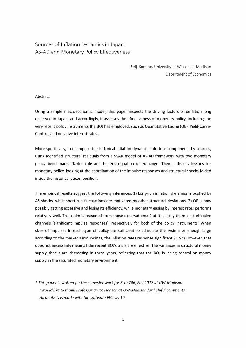
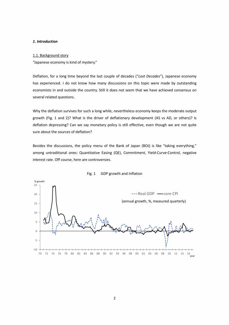
Why the deflation survives for such a long while, nevertheless economy keeps the moderate output
growth (Fig. 1 and 2)? What is the driver of deflationary development (AS vs AD, or others)? Is
deflation depressing? Can we say monetary policy is still effective, even though we are not quite
sure about the sources of deflation?
Besides the discussions, the policy menu of the Bank of Japan (BOJ) is like “taking everything,”
among untraditional ones: Quantitative Easing (QE), Commitment, Yield-Curve-Control, negative
interest rate. Off course, here are controversies.
Fig. 1 GDP growth and Inflation
-10
-5
0
5
10
15
20
25
70 72 74 76 78 80 82 84 86 88 90 92 94 96 98 00 02 04 06 08 10 12 14 16
Real GDP core CPI
(annual growth, %, measured quarterly)
year
% growth
3
Fig. 2 Inflation vs GDP growth, by periods (quarterly % chg.)
1.2. Purpose of research
This paper aims to answer two questions: 1) What is the driving factor of Japanese deflation? 2)
Was monetary policy effective so far, and is it even now? In the way I try to sublate the polarizing
views from supply-side school (or hawks in monetary policy) and demand-side school (doves, or
reflationists). Using a simple macroeconomic model, this paper inspects the driving factors of
deflation long observed in Japan, and accordingly, it assesses the effectiveness of monetary policy,
including the very recent policy instruments BOJ has employed, such as Quantitative Easing, Yield-
Curve-Control, and negative interest rates.
More specifically, I decompose the historical inflation dynamics into four components by sources [:
AS shocks, AD shocks, MD shocks, and MS shocks1], using identified structural residuals from a
SVAR model (system of four endogenous [y, p, r, m]) of AS-AD framework with two monetary policy
benchmarks: Taylor rule and Fisher’s equation of exchange. Then, I discuss lessons for monetary
policy, looking at the coordination of the impulse responses and structural shocks folded inside the
historical decomposition.
1.3. Literature
There are numbers of studies on this topic and approach. Gali (1992) was a pathfinder of this
literature. He empirically analyzed the four variables VAR model ―that is [y, p, r, m], as well as me―
for the U.S. data with monetary policy assessments. Gerlach and Smets (1995) investigated three
variables VAR (excepting for money supply), to see the effects of interest rate shocks in G-7
countries during the period 1979-1993. They observed inflation rate in Japan dropped in the late
80’s due to AD shocks, and then bounced up as the results of monetary easing. Mio (2003), focusing
on a simple AS-AD with a two variables system for Japan up to 1999, reported both of AS and AD
1 Respectively, aggregate demand, aggregate supply, money demand, and money supply.
-5
0
5
10
15
20
25
30
-4 -2 0 2 4 6 8 10 12
Inflation vs GDP growth (1971Q1-1994Q4)% chg.
% chg.-3
-2
-1
0
1
2
3
4
5
-10 -8 -6 -4 -2 0 2 4 6 8
Inflation vs GDP growth (1995Q1-2017Q2)% chg.
% chg.
4
disturbances played non-negligible roles on disinflation in the 90’s. Monetary policy was not
assessed there.
1.4. Merits of this paper
A virtue of the approach in this series of studies is that we can have a single analytical platform
which synthesizes causal inductions of inflation dynamics and assessments of policy effects.
In addition, let me point out, compared with those predecessors, my research has the following
advantages:
1) Analyze both of two types of monetary policy: interest rate and quantity.
2) Use of long-term interest rate to capture the current policy trials on yield curves (The papers
above used short-term interbank rates).
3) Including recent data, the periods of unconventional policy.
4) Also, rather older data. In many studies with standard 10-year JGB yields for Japan, the sample
starts from the late 80’s, due to data availability2. I pick 9-year JGB as interest rate which is
obtained from 1973. For my historical decomposition analysis, it is essential to big have episodes
such as oil-shock and financial bubble during the 70-80’s.
2 I mean here that 10-year compound index obtained from Bloomberg starts from the mid 80’s.
5
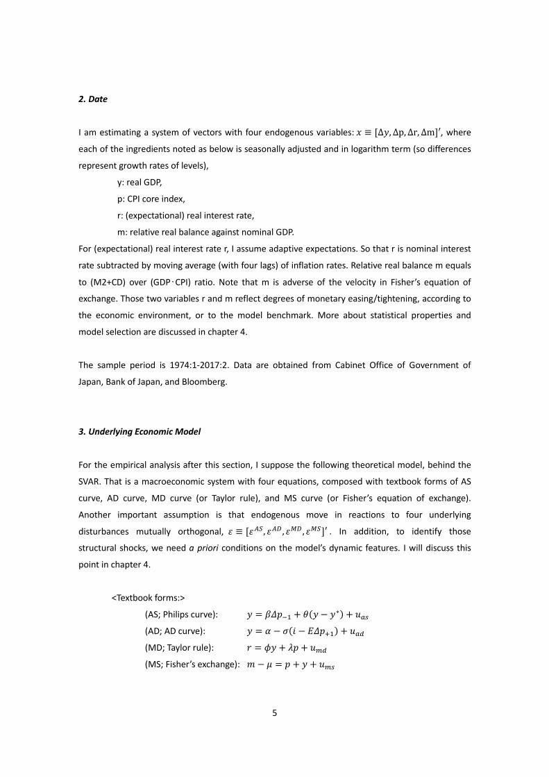
2. Date
I am estimating a system of vectors with four endogenous variables: 𝑥𝑥 ≡ [∆𝑦𝑦,∆p,∆r,∆m]′, where
each of the ingredients noted as below is seasonally adjusted and in logarithm term (so differences
represent growth rates of levels),
y: real GDP,
p: CPI core index,
r: (expectational) real interest rate,
m: relative real balance against nominal GDP.
For (expectational) real interest rate r, I assume adaptive expectations. So that r is nominal interest
rate subtracted by moving average (with four lags) of inflation rates. Relative real balance m equals
to (M2+CD) over (GDP∙CPI) ratio. Note that m is adverse of the velocity in Fisher’s equation of
exchange. Those two variables r and m reflect degrees of monetary easing/tightening, according to
the economic environment, or to the model benchmark. More about statistical properties and
model selection are discussed in chapter 4.
The sample period is 1974:1-2017:2. Data are obtained from Cabinet Office of Government of
Japan, Bank of Japan, and Bloomberg.
3. Underlying Economic Model
For the empirical analysis after this section, I suppose the following theoretical model, behind the
SVAR. That is a macroeconomic system with four equations, composed with textbook forms of AS
curve, AD curve, MD curve (or Taylor rule), and MS curve (or Fisher’s equation of exchange).
Another important assumption is that endogenous move in reactions to four underlying
disturbances mutually orthogonal, 𝜀𝜀 ≡ [𝜀𝜀𝐴𝐴𝐴𝐴, 𝜀𝜀𝐴𝐴𝐴𝐴 , 𝜀𝜀𝑀𝑀𝐴𝐴 , 𝜀𝜀𝑀𝑀𝐴𝐴]′ . In addition, to identify those
structural shocks, we need a priori conditions on the model’s dynamic features. I will discuss this
point in chapter 4.
<Textbook forms:>
(AS; Philips curve): 𝑦𝑦 = 𝛽𝛽𝛽𝛽𝑝𝑝−1 + 𝜃𝜃(𝑦𝑦 − 𝑦𝑦∗) + 𝑢𝑢𝑎𝑎𝑎𝑎
(AD; AD curve): 𝑦𝑦 = 𝛼𝛼 − 𝜎𝜎(𝑖𝑖 − 𝐸𝐸𝛽𝛽𝑝𝑝+1) + 𝑢𝑢𝑎𝑎𝑎𝑎
(MD; Taylor rule): 𝑟𝑟 = 𝜙𝜙𝑦𝑦 + 𝜆𝜆𝑝𝑝 + 𝑢𝑢𝑚𝑚𝑎𝑎
(MS; Fisher’s exchange): 𝑚𝑚− 𝜇𝜇 = 𝑝𝑝 + 𝑦𝑦 + 𝑢𝑢𝑚𝑚𝑎𝑎

6
4. Empirical Method
Before estimating a system, to certify I have a covariance stationary vector process, I investigate the
time-series properties of each variables. As a result, I will take first differential formation
𝑥𝑥 ≡ [∆𝑦𝑦,∆p,∆r,∆m]′ in the SVAR estimation.
4.1. Unit root and cointegration tests
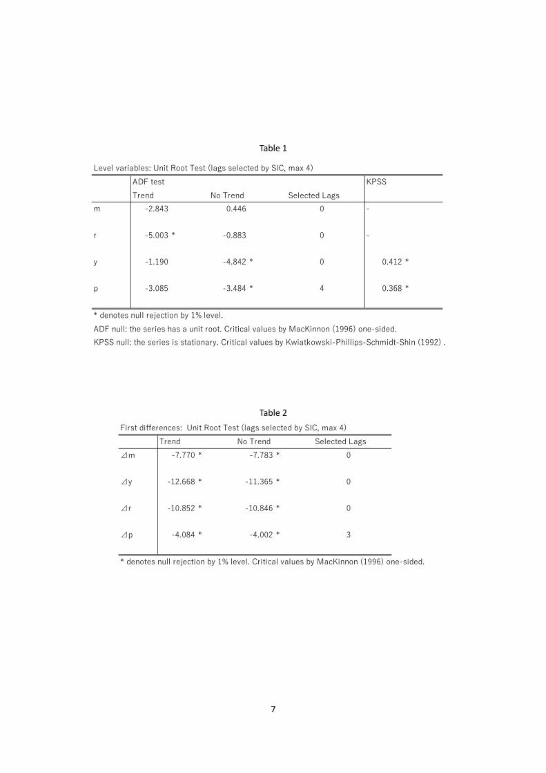
Table 1 summarizes the outcomes of unit root tests for level variables. At first, I examine unit root
of each level variable by Augmented Dickey-Fuller test (1979). In the table, there are shown both
results from tests with trend and without trend. Shortly, we can say m is nonstationary. On the
other hand, hypothesis of r’s unit root is rejected when a time trend is included. I interpret r is
trend-stationary process (TSP), supported by that the coefficient on the trend term was significant.
Anyway, I use Δr in SVAR analysis to eliminate the linear trend. Series y and p need an additional
step. ADF tests with trend did not reject unit roots, while those with trend did, suggesting
possibilities of non-stationarity. The powers of those tests, however, are presumably low, because
estimators on lagged terms were very close to 1 (0.99 for y, 0.96 for p). Thereat, I employ
Kwiatkowski-Phillips-Schmidt-Shin (1992) (KPSS) tests for y and p in a supplemental way, resulting in
rejections null hypothesis that they are stationary3. Thus, a plausible view is that the two series are
family of random walk. Also, it is confirmed there are no unit roots in first differences of all variables
by ADF tests (Table 2).
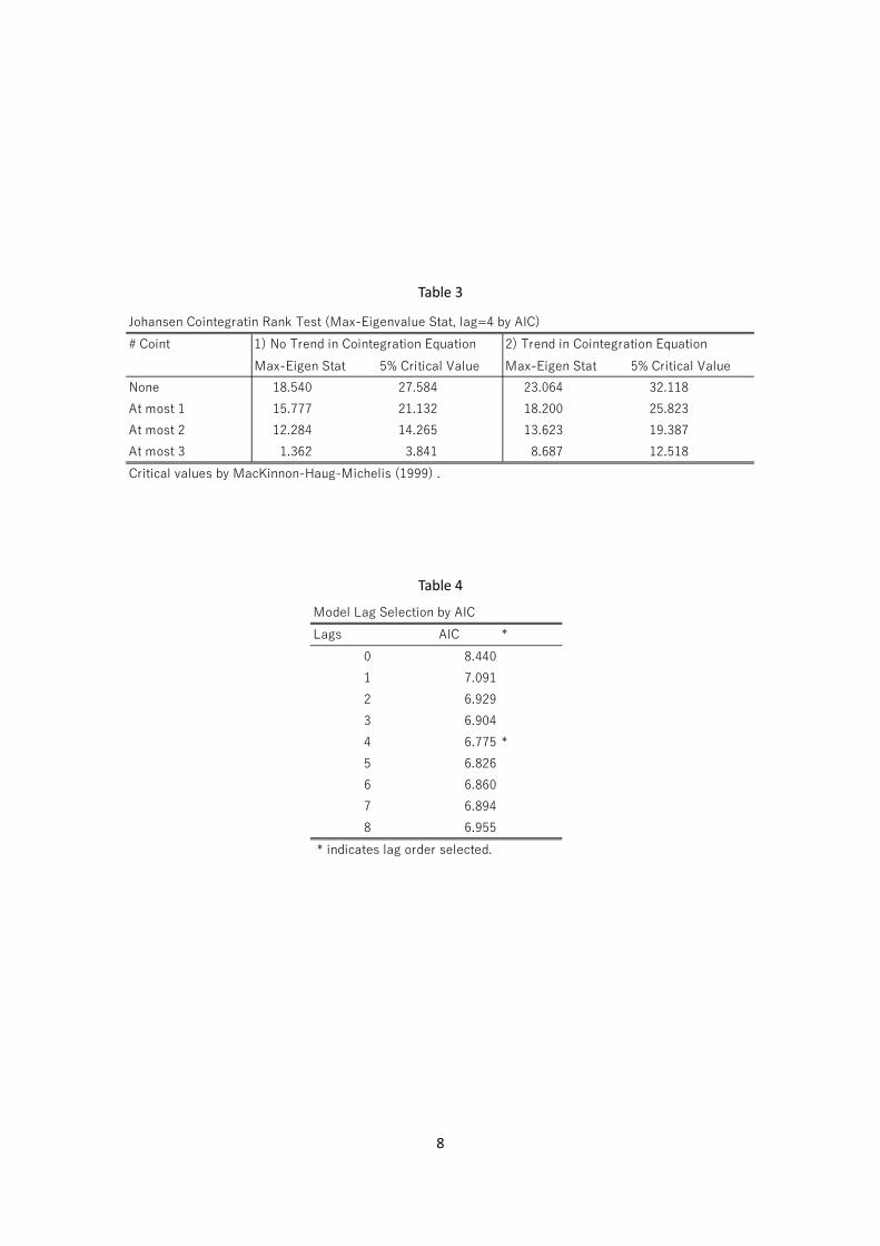
After checking unit roots, possibilities of cointegrations are tested, with Johansen and Juselius’s
(1990) maximum eigenvalue statistics. As reported in Table 3, the system is not likely a cointegrated
process. In this test, four lags are chosen by AIC, also in the forthcoming SVAR estimation (Table 4).
So, again, the system to estimate below is of 𝑥𝑥 ≡ [∆𝑦𝑦,∆p,∆r,∆m]′ with four lags.
3 Note that the design of null and counter hypothesis in KPSS test is reversed to Dickey-Fuller.
7
Table 1
Table 2
Level variables: Unit Root Test (lags selected by SIC, max 4)ADF test KPSSTrend No Trend Selected Lags
m -2.843 0.446 0 -
r -5.003 * -0.883 0 -
y -1.190 -4.842 * 0 0.412 *
p -3.085 -3.484 * 4 0.368 *
* denotes null rejection by 1% level.ADF null: the series has a unit root. Critical values by MacKinnon (1996) one-sided.KPSS null: the series is stationary. Critical values by Kwiatkowski-Phillips-Schmidt-Shin (1992) .
First differences: Unit Root Test (lags selected by SIC, max 4)Trend No Trend Selected Lags
⊿m -7.770 * -7.783 * 0
⊿y -12.668 * -11.365 * 0
⊿r -10.852 * -10.846 * 0
⊿p -4.084 * -4.002 * 3
* denotes null rejection by 1% level. Critical values by MacKinnon (1996) one-sided.
8
Table 3
Table 4
Johansen Cointegratin Rank Test (Max-Eigenvalue Stat, lag=4 by AIC)# Coint 1) No Trend in Cointegration Equation 2) Trend in Cointegration Equation
Max-Eigen Stat 5% Critical Value Max-Eigen Stat 5% Critical ValueNone 18.540 27.584 23.064 32.118At most 1 15.777 21.132 18.200 25.823At most 2 12.284 14.265 13.623 19.387At most 3 1.362 3.841 8.687 12.518Critical values by MacKinnon-Haug-Michelis (1999) .
Model Lag Selection by AICLags AIC *
0 8.4401 7.0912 6.9293 6.9044 6.775 *5 6.8266 6.8607 6.8948 6.955
* indicates lag order selected.
9
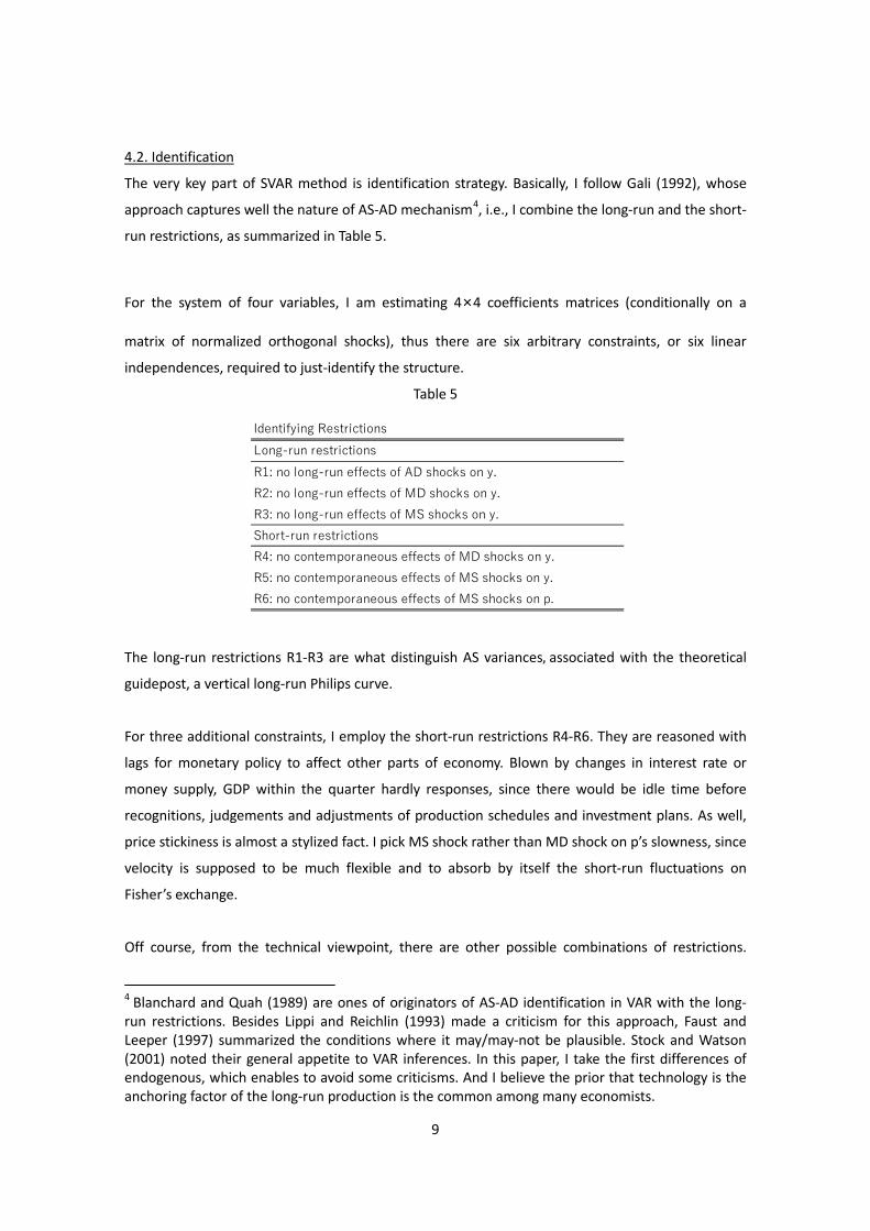
4.2. Identification
The very key part of SVAR method is identification strategy. Basically, I follow Gali (1992), whose
approach captures well the nature of AS-AD mechanism4, i.e., I combine the long-run and the short-
run restrictions, as summarized in Table 5.
For the system of four variables, I am estimating 4×4 coefficients matrices (conditionally on a
matrix of normalized orthogonal shocks), thus there are six arbitrary constraints, or six linear
independences, required to just-identify the structure.
Table 5
The long-run restrictions R1-R3 are what distinguish AS variances, associated with the theoretical
guidepost, a vertical long-run Philips curve.
For three additional constraints, I employ the short-run restrictions R4-R6. They are reasoned with
lags for monetary policy to affect other parts of economy. Blown by changes in interest rate or
money supply, GDP within the quarter hardly responses, since there would be idle time before
recognitions, judgements and adjustments of production schedules and investment plans. As well,
price stickiness is almost a stylized fact. I pick MS shock rather than MD shock on p’s slowness, since
velocity is supposed to be much flexible and to absorb by itself the short-run fluctuations on
Fisher’s exchange.
Off course, from the technical viewpoint, there are other possible combinations of restrictions.
4 Blanchard and Quah (1989) are ones of originators of AS-AD identification in VAR with the long-run restrictions. Besides Lippi and Reichlin (1993) made a criticism for this approach, Faust and Leeper (1997) summarized the conditions where it may/may-not be plausible. Stock and Watson (2001) noted their general appetite to VAR inferences. In this paper, I take the first differences of endogenous, which enables to avoid some criticisms. And I believe the prior that technology is the anchoring factor of the long-run production is the common among many economists.
Identifying RestrictionsLong-run restrictionsR1: no long-run effects of AD shocks on y.R2: no long-run effects of MD shocks on y.R3: no long-run effects of MS shocks on y.Short-run restrictionsR4: no contemporaneous effects of MD shocks on y.R5: no contemporaneous effects of MS shocks on y.R6: no contemporaneous effects of MS shocks on p.
10
However, from qualitative priors, it is not so plausible to have constraints on reactions of r and m,
since the financial market adapts very quickly to surprises.
4.3. Econometrical expressions
The VAR system has several formularizations. As noted, our system is of 𝑥𝑥 ≡ [∆𝑦𝑦,∆p,∆r,∆m]′,
whose dynamics are driven by structural disturbances 𝜀𝜀 ≡ [𝜀𝜀𝐴𝐴𝐴𝐴, 𝜀𝜀𝐴𝐴𝐴𝐴, 𝜀𝜀𝑀𝑀𝐴𝐴, 𝜀𝜀𝑀𝑀𝐴𝐴]′, which are mutually
orthogonal.
The MA representation of the structural form is,
𝑥𝑥 = 𝐶𝐶(𝐿𝐿)𝜀𝜀,
where 𝐶𝐶(𝐿𝐿) ≡ �𝐶𝐶(𝐿𝐿)𝑖𝑖𝑖𝑖�,𝑓𝑓𝑓𝑓𝑟𝑟 𝑖𝑖, 𝑗𝑗 = 1, 2, 3, 4.
We can also write Wold MA reduced form,
𝑥𝑥 = 𝐸𝐸(𝐿𝐿)𝑣𝑣,
where 𝐸𝐸(𝐿𝐿) ≡ �𝐸𝐸(𝐿𝐿)𝑖𝑖𝑖𝑖�,𝑓𝑓𝑓𝑓𝑟𝑟 𝑖𝑖, 𝑗𝑗 = 1, 2, 3, 4, 𝐸𝐸(0) = 𝐼𝐼, 𝑎𝑎𝑎𝑎𝑎𝑎 𝐸𝐸(𝐿𝐿) 𝑖𝑖𝑖𝑖 𝑖𝑖𝑎𝑎𝑣𝑣𝑖𝑖𝑟𝑟𝑖𝑖𝑖𝑖𝑖𝑖𝑖𝑖𝑖𝑖. Innovations are
defined by 𝑣𝑣 ≡ 𝑥𝑥 − 𝑃𝑃[𝑥𝑥|𝑥𝑥(−1),𝑥𝑥(−2), … ], where P is the orthogonal projection operator, with the
variance-covariance matrix Σ ≡ 𝐸𝐸𝑣𝑣𝑣𝑣′.
Then we have an AR expression of the reduced form,
𝐵𝐵(𝐿𝐿) 𝑥𝑥 = 𝑣𝑣,
where 𝐵𝐵(𝐿𝐿) ≡ �𝐵𝐵(𝐿𝐿)𝑖𝑖𝑖𝑖�,𝑓𝑓𝑓𝑓𝑟𝑟 𝑖𝑖, 𝑗𝑗 = 1, 2, 3, 4,𝐸𝐸(0) = 𝐼𝐼,𝑎𝑎𝑎𝑎𝑎𝑎 𝐵𝐵(𝐿𝐿) = 𝐸𝐸(𝐿𝐿)−1.
By finding a 4×4 matrix S such that 𝑣𝑣 = 𝑆𝑆𝜀𝜀 and thus 𝑃𝑃[𝜀𝜀|𝑥𝑥(−1),𝑥𝑥(−2), … ] = 0, 𝑗𝑗 ≥ 1, and
𝐶𝐶(𝐿𝐿) = 𝐸𝐸(𝐿𝐿)𝑆𝑆, we acquire AR form of the structure,
𝐴𝐴(𝐿𝐿) 𝑥𝑥 = 𝜀𝜀,
where 𝐴𝐴(𝐿𝐿) ≡ �𝐴𝐴(𝐿𝐿)𝑖𝑖𝑖𝑖�,𝑓𝑓𝑓𝑓𝑟𝑟 𝑖𝑖, 𝑗𝑗 = 1, 2, 3, 4,𝑎𝑎𝑎𝑎𝑎𝑎 𝐴𝐴(0) ≡ 𝑆𝑆−1.
In a normalized version of shocks, 𝐸𝐸𝜀𝜀𝜀𝜀′ = I, so SS′ = Σ, accompanied by ten conditions.
To just-identify the structure, my six restrictions are imposed in the following ways.
The long-run constraints R1, R2 and R3 correspond to:
𝐶𝐶12(1) = 𝐶𝐶13(1) = 𝐶𝐶14(1) = 0.
Or equivalently,
𝐸𝐸11(1)𝑆𝑆12 + 𝐸𝐸12(1)𝑆𝑆22 + 𝐸𝐸13(1)𝑆𝑆32 + 𝐸𝐸14(1)𝑆𝑆42 = 0,
𝐸𝐸11(1)𝑆𝑆13 + 𝐸𝐸12(1)𝑆𝑆23 + 𝐸𝐸13(1)𝑆𝑆33 + 𝐸𝐸14(1)𝑆𝑆43 = 0,
𝐸𝐸11(1)𝑆𝑆14 + 𝐸𝐸12(1)𝑆𝑆24 + 𝐸𝐸13(1)𝑆𝑆34 + 𝐸𝐸14(1)𝑆𝑆44 = 0.
11
Also, the short-run restrictions R4-R6 require:
𝑆𝑆13 = 𝑆𝑆14 = 𝑆𝑆24 = 0.
5. Results
5.1. Guideline of chapter 5
In this chapter, I introduce the results of empirical analysis, along the following outline. Section 5.2
focuses on identified structural shocks. I check they are reasonably decomposed into economic
factors, as well as I brief how they have moved according to the history. Impulse responses are
inspected in the following section 5.3, depicting the way Japanese economy behaves in reactions to
the certain variances, on average within the sample periods. Then, section 5.4 is about the results
of historical decompositions, which reveals how the shocks were propagated thorough the impulse
responses into chronological developments of macro variables. Robustness of the results are
checked in Appendix.
Going through the stroke, a set of possible answers will be suggested for the questions I set in the
beginning. Again, those are questions of: 1) the driving factor of Japanese deflation; 2) monetary
policy effectiveness (in the past and current).
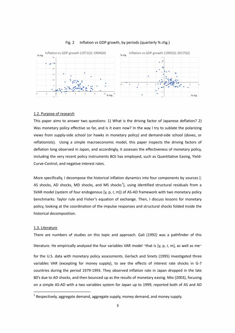
I believe it is helpful for further discussions to notice here this paper’s strategy of assessment on
policy effectiveness. That can be evaluated by three stages, as Fig. 3 illustrates. 1) At first, we should
examine if enough stimulus―sufficient according to the economic environment― were made on
policy instruments. This point includes the authority’s ability to control policy tools as intended. 2)
Second, we need to know there exist channels which transmit the policy effects into the system. 3)
Finally, both information is folded in one place, the total effectiveness. In the empirics, those three
stages correspond respectively to 1) structural deviations, 2) impulse responses, and 3) historical
decompositions.
Fig. 3
12
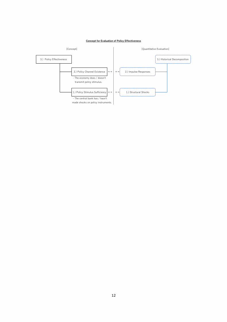
- The economy does / doesn't transmit policy stimulus.
- The central bank has / hasn't made shocks on policy instruments.
Concept for Evaluation of Policy Effectiveness
[Concept] [Quantitative Evaluation]
⇒⇒ ⇒⇒
3.) Historical Decomposition 3.)Policy Effectiveness
2.) Policy Channel Existence
1.) Policy Stimulus Sufficiency
2.) Impulse Responses
1.) Structural Shocks
⇒⇒ ⇒⇒
13
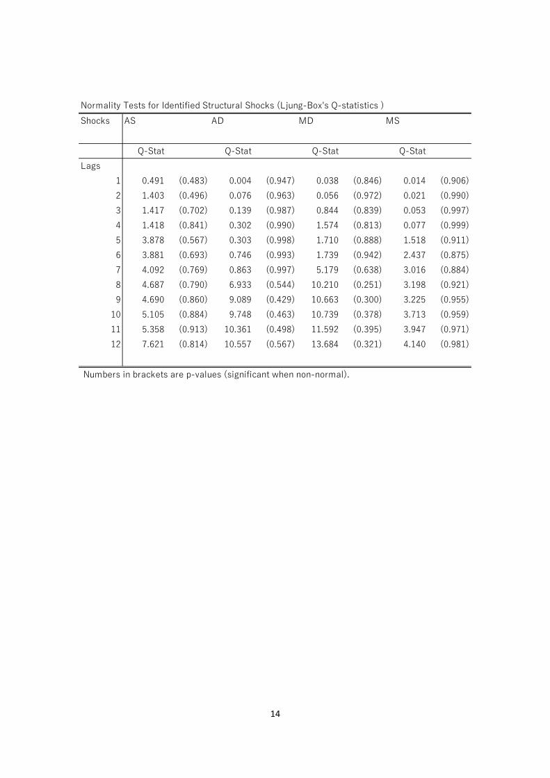
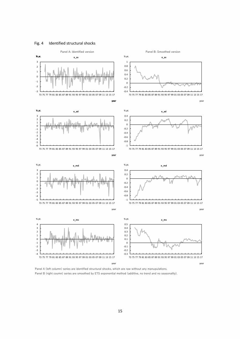
5.2. Identified structural shocks
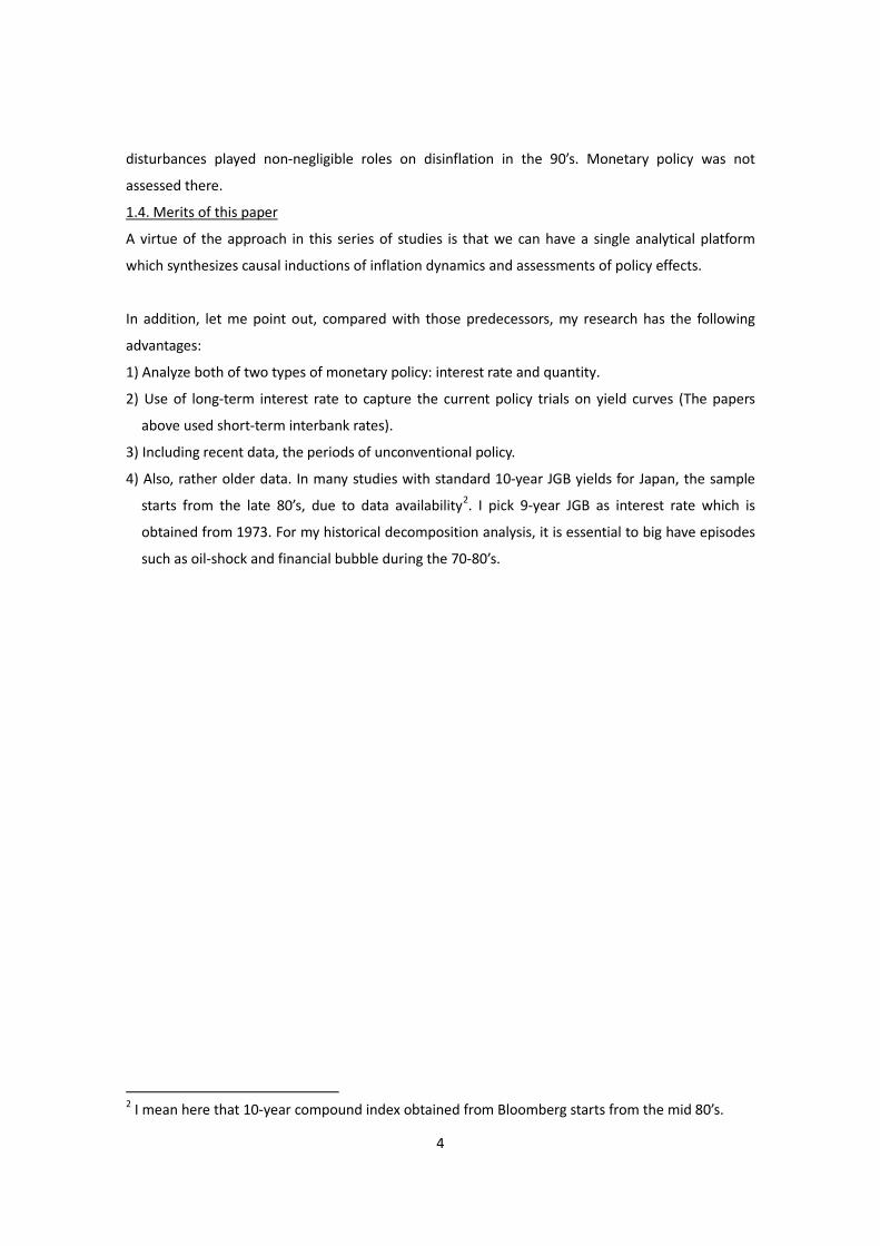
The SVAR with the noted specifications reports the structural shocks as in Fig. 4-Panel A (left
column). It is seen that this stochastics is zero-mean, stable variance process, as tested by Ljung-
Box’s Q-stats as in Table 6. Fig. 4-Panel B (right column) plots the smoothed version by ETS
exponential smoothing (Hyndman, et al., 2002)5, which is for a supplemental reference to grab their
historical characteristics (Note that their appearances are relying upon transitions of the mid-term
mean, so just focus the big picture of momentum6). AS deviation dropped sharply at two oil-shocks
in the 70’s and the credit crisis in 1991-1993. AD shock grew rapidly in the 70’s, but it slowed down
in the late 80’s, corresponding to the end of the financial boom, and stagnated during the Lost
Decades. We can also find the collapses in 2001 and 2009. MS showed similar movement as AD, but
it became flatter after declining by the 90’s credit crunch. Meanwhile, MS behaved somehow
oppositely to MS, losing its initial height through the bubble economy.
Table 6
5 Spec: additive, no trend and no seasonality. 6 It is understandable if it is thought the appearances of Panel B invokes they would have a sort of
mid-term trends. Technologically speaking, however, it does not necessarily imply that (by the nature of ETS smoothing method). Even if it does, the normality of residuals holds at least in the long horizon, as tested in Table 6. Anyhow, I use this here for a brief characterization, as mentioned.
14
Normality Tests for Identified Structural Shocks (Ljung-Box's Q-statistics )Shocks AS AD MD MS
Q-Stat Q-Stat Q-Stat Q-StatLags
1 0.491 (0.483) 0.004 (0.947) 0.038 (0.846) 0.014 (0.906)2 1.403 (0.496) 0.076 (0.963) 0.056 (0.972) 0.021 (0.990)3 1.417 (0.702) 0.139 (0.987) 0.844 (0.839) 0.053 (0.997)4 1.418 (0.841) 0.302 (0.990) 1.574 (0.813) 0.077 (0.999)5 3.878 (0.567) 0.303 (0.998) 1.710 (0.888) 1.518 (0.911)6 3.881 (0.693) 0.746 (0.993) 1.739 (0.942) 2.437 (0.875)7 4.092 (0.769) 0.863 (0.997) 5.179 (0.638) 3.016 (0.884)8 4.687 (0.790) 6.933 (0.544) 10.210 (0.251) 3.198 (0.921)9 4.690 (0.860) 9.089 (0.429) 10.663 (0.300) 3.225 (0.955)
10 5.105 (0.884) 9.748 (0.463) 10.739 (0.378) 3.713 (0.959)11 5.358 (0.913) 10.361 (0.498) 11.592 (0.395) 3.947 (0.971)12 7.621 (0.814) 10.557 (0.567) 13.684 (0.321) 4.140 (0.981)
Numbers in brackets are p-values (significant when non-normal).
15
Fig. 4 Identified structural shocks
Panel A: Identified version Panel B: Smoothed version
Panel A (left column) series are identified structural shocks, which are raw without any manupulations. Panel B (right coumn) series are smoothed by ETS exponential method (additive, no trend and no seasonality).
-3
-2
-1
0
1
2
3
73 75 77 79 81 83 85 87 89 91 93 95 97 99 01 03 05 07 09 11 13 15 17
e_as% pt.
year
% pt.
year
% pt.
year
% pt.
year
-1
-0.8
-0.6
-0.4
-0.2
0
0.2
0.4
73 75 77 79 81 83 85 87 89 91 93 95 97 99 01 03 05 07 09 11 13 15 17
e_md% pt.
year
-0.3-0.2-0.1
00.10.20.30.40.5
73 75 77 79 81 83 85 87 89 91 93 95 97 99 01 03 05 07 09 11 13 15 17
e_ms% pt.
year
-1
-0.8
-0.6
-0.4
-0.2
0
0.2
0.4
73 75 77 79 81 83 85 87 89 91 93 95 97 99 01 03 05 07 09 11 13 15 17
e_ad% pt.
year
-6-5-4-3-2-10123
73 75 77 79 81 83 85 87 89 91 93 95 97 99 01 03 05 07 09 11 13 15 17
e_ad% pt.
year
% pt.
year
-5-4-3-2-10123
73 75 77 79 81 83 85 87 89 91 93 95 97 99 01 03 05 07 09 11 13 15 17
e_md% pt.
year
-4-3-2-101234
73 75 77 79 81 83 85 87 89 91 93 95 97 99 01 03 05 07 09 11 13 15 17
e_ms% pt.
year
-0.4
-0.2
0
0.2
0.4
0.6
0.8
1
73 75 77 79 81 83 85 87 89 91 93 95 97 99 01 03 05 07 09 11 13 15 17
e_as% pt.
year
16
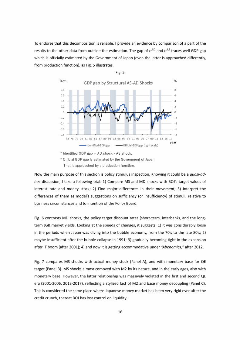
To endorse that this decomposition is reliable, I provide an evidence by comparison of a part of the
results to the other data from outside the estimation. The gap of 𝜀𝜀𝐴𝐴𝐴𝐴 and 𝜀𝜀𝐴𝐴𝐴𝐴 traces well GDP gap
which is officially estimated by the Government of Japan (even the latter is approached differently,
from production function), as Fig. 5 illustrates.
Fig. 5
Now the main purpose of this section is policy stimulus inspection. Knowing it could be a quasi-ad-
hoc discussion, I take a following trial: 1) Compare MS and MD shocks with BOJ’s target values of
interest rate and money stock; 2) Find major differences in their movement; 3) Interpret the
differences of them as model’s suggestions on sufficiency (or insufficiency) of stimuli, relative to
business circumstances and to intention of the Policy Board.
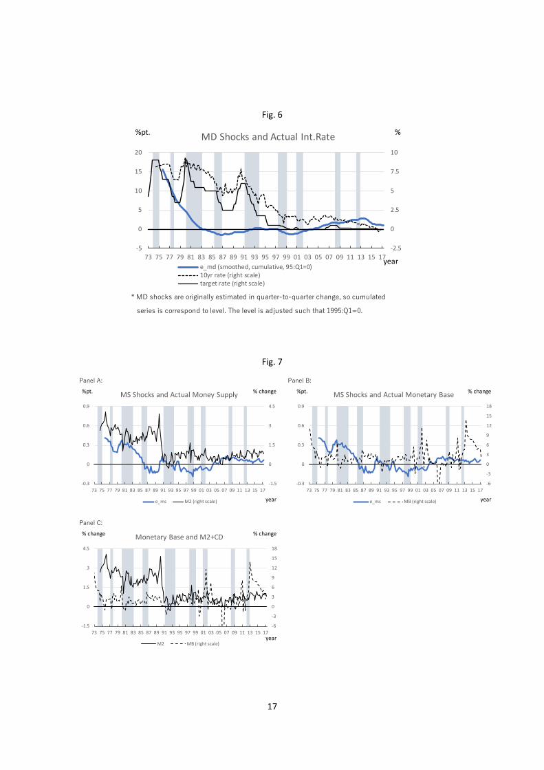
Fig. 6 contrasts MD shocks, the policy target discount rates (short-term, interbank), and the long-
term JGB market yields. Looking at the speeds of changes, it suggests: 1) it was considerably loose
in the periods when Japan was diving into the bubble economy, from the 70’s to the late 80’s; 2)
maybe insufficient after the bubble collapse in 1991; 3) gradually becoming tight in the expansion
after IT boom (after 2001); 4) and now it is getting accommodative under “Abenomics,” after 2012.
Fig. 7 compares MS shocks with actual money stock (Panel A), and with monetary base for QE
target (Panel B). MS shocks almost comoved with M2 by its nature, and in the early ages, also with
monetary base. However, the latter relationship was massively violated in the first and second QE
era (2001-2006, 2013-2017), reflecting a stylized fact of M2 and base money decoupling (Panel C).
This is considered the same place where Japanese money market has been very rigid ever after the
credit crunch, thereat BOJ has lost control on liquidity.
* Identified GDP gap = AD shock - AS shock. * Official GDP gap is estimated by the Government of Japan. That is approached by a production function.
-8
-6
-4
-2
0
2
4
6
8
-0.8
-0.6
-0.4
-0.2
0
0.2
0.4
0.6
0.8
73 75 77 79 81 83 85 87 89 91 93 95 97 99 01 03 05 07 09 11 13 15 17
GDP gap by Structural AS-AD Shocks
Identified GDP gap Official GDP gap (right scale)
%pt. %
year
17
Fig. 6
Fig. 7
* MD shocks are originally estimated in quarter-to-quarter change, so cumulated
series is correspond to level. The level is adjusted such that 1995:Q1=0.
-2.5
0
2.5
5
7.5
10
-5
0
5
10
15
20
73 75 77 79 81 83 85 87 89 91 93 95 97 99 01 03 05 07 09 11 13 15 17
MD Shocks and Actual Int.Rate
e_md (smoothed, cumulative, 95:Q1=0)10yr rate (right scale)target rate (right scale)
%pt. %
year
Panel A: Panel B:
Panel C:
-6
-3
0
3
6
9
12
15
18
-1.5
0
1.5
3
4.5
73 75 77 79 81 83 85 87 89 91 93 95 97 99 01 03 05 07 09 11 13 15 17
Monetary Base and M2+CD
M2 MB (right scale)
% change % change
year
-6
-3
0
3
6
9
12
15
18
-0.3
0
0.3
0.6
0.9
73 75 77 79 81 83 85 87 89 91 93 95 97 99 01 03 05 07 09 11 13 15 17
MS Shocks and Actual Monetary Base
e_ms MB (right scale)
%pt. % change
year
-1.5
0
1.5
3
4.5
-0.3
0
0.3
0.6
0.9
73 75 77 79 81 83 85 87 89 91 93 95 97 99 01 03 05 07 09 11 13 15 17
MS Shocks and Actual Money Supply
e_ms M2 (right scale)
%pt. % change
year
18
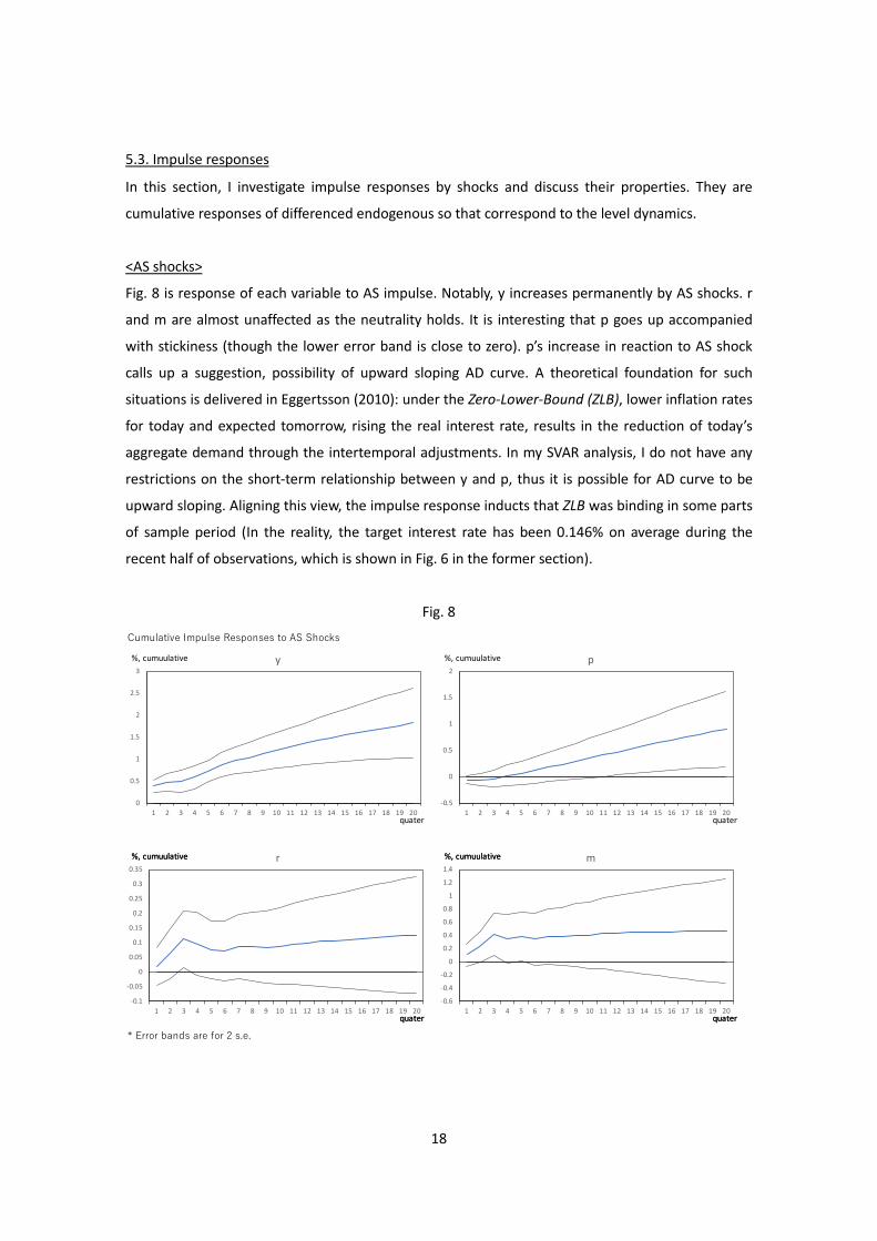
5.3. Impulse responses
In this section, I investigate impulse responses by shocks and discuss their properties. They are
cumulative responses of differenced endogenous so that correspond to the level dynamics.
<AS shocks>
Fig. 8 is response of each variable to AS impulse. Notably, y increases permanently by AS shocks. r
and m are almost unaffected as the neutrality holds. It is interesting that p goes up accompanied
with stickiness (though the lower error band is close to zero). p’s increase in reaction to AS shock
calls up a suggestion, possibility of upward sloping AD curve. A theoretical foundation for such
situations is delivered in Eggertsson (2010): under the Zero-Lower-Bound (ZLB), lower inflation rates
for today and expected tomorrow, rising the real interest rate, results in the reduction of today’s
aggregate demand through the intertemporal adjustments. In my SVAR analysis, I do not have any
restrictions on the short-term relationship between y and p, thus it is possible for AD curve to be
upward sloping. Aligning this view, the impulse response inducts that ZLB was binding in some parts
of sample period (In the reality, the target interest rate has been 0.146% on average during the
recent half of observations, which is shown in Fig. 6 in the former section).
Fig. 8
Cumulative Impulse Responses to AS Shocks
* Error bands are for 2 s.e.
0
0.5
1
1.5
2
2.5
3
1 2 3 4 5 6 7 8 9 10 11 12 13 14 15 16 17 18 19 20
y%, cumuulative
quater
-0.5
0
0.5
1
1.5
2
1 2 3 4 5 6 7 8 9 10 11 12 13 14 15 16 17 18 19 20
p%, cumuulative
quater
-0.1
-0.05
0
0.05
0.1
0.15
0.2
0.25
0.3
0.35
1 2 3 4 5 6 7 8 9 10 11 12 13 14 15 16 17 18 19 20
r%, cumuulative
quater
%, cumuulative
quater
-0.6
-0.4
-0.2
0
0.2
0.4
0.6
0.8
1
1.2
1.4
1 2 3 4 5 6 7 8 9 10 11 12 13 14 15 16 17 18 19 20
m%, cumuulative
quater
%, cumuulative
quater
19
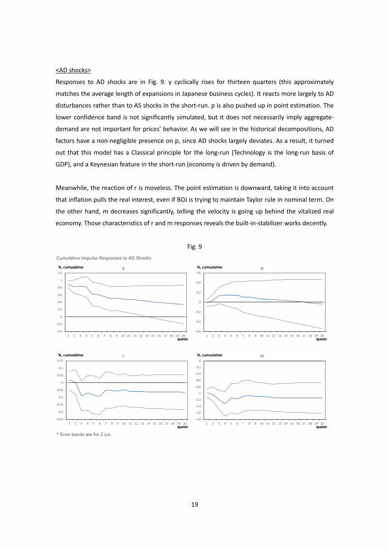
<AD shocks>
Responses to AD shocks are in Fig. 9. y cyclically rises for thirteen quarters (this approximately
matches the average length of expansions in Japanese business cycles). It reacts more largely to AD
disturbances rather than to AS shocks in the short-run. p is also pushed up in point estimation. The
lower confidence band is not significantly simulated, but it does not necessarily imply aggregate-
demand are not important for prices’ behavior. As we will see in the historical decompositions, AD
factors have a non-negligible presence on p, since AD shocks largely deviates. As a result, it turned
out that this model has a Classical principle for the long-run (Technology is the long-run basis of
GDP), and a Keynesian feature in the short-run (economy is driven by demand).
Meanwhile, the reaction of r is moveless. The point estimation is downward, taking it into account
that inflation pulls the real interest, even if BOJ is trying to maintain Taylor rule in nominal term. On
the other hand, m decreases significantly, telling the velocity is going up behind the vitalized real
economy. Those characteristics of r and m responses reveals the built-in-stabilizer works decently.
Fig. 9
Cumulative Impulse Responses to AD Shocks
* Error bands are for 2 s.e.
-0.4
-0.2
0
0.2
0.4
0.6
0.8
1
1.2
1 2 3 4 5 6 7 8 9 10 11 12 13 14 15 16 17 18 19 20
y%, cumuulative
quater
%, cumuulative
quater
-0.6
-0.4
-0.2
0
0.2
0.4
0.6
1 2 3 4 5 6 7 8 9 10 11 12 13 14 15 16 17 18 19 20
p%, cumuulative
quater
%, cumuulative
quater
-0.25
-0.2
-0.15
-0.1
-0.05
0
0.05
0.1
0.15
1 2 3 4 5 6 7 8 9 10 11 12 13 14 15 16 17 18 19 20
r%, cumuulative
quater
%, cumuulative
quater
-1.8
-1.6
-1.4
-1.2
-1
-0.8
-0.6
-0.4
-0.2
0
1 2 3 4 5 6 7 8 9 10 11 12 13 14 15 16 17 18 19 20
m%, cumuulative
quater
%, cumuulative
quater
20
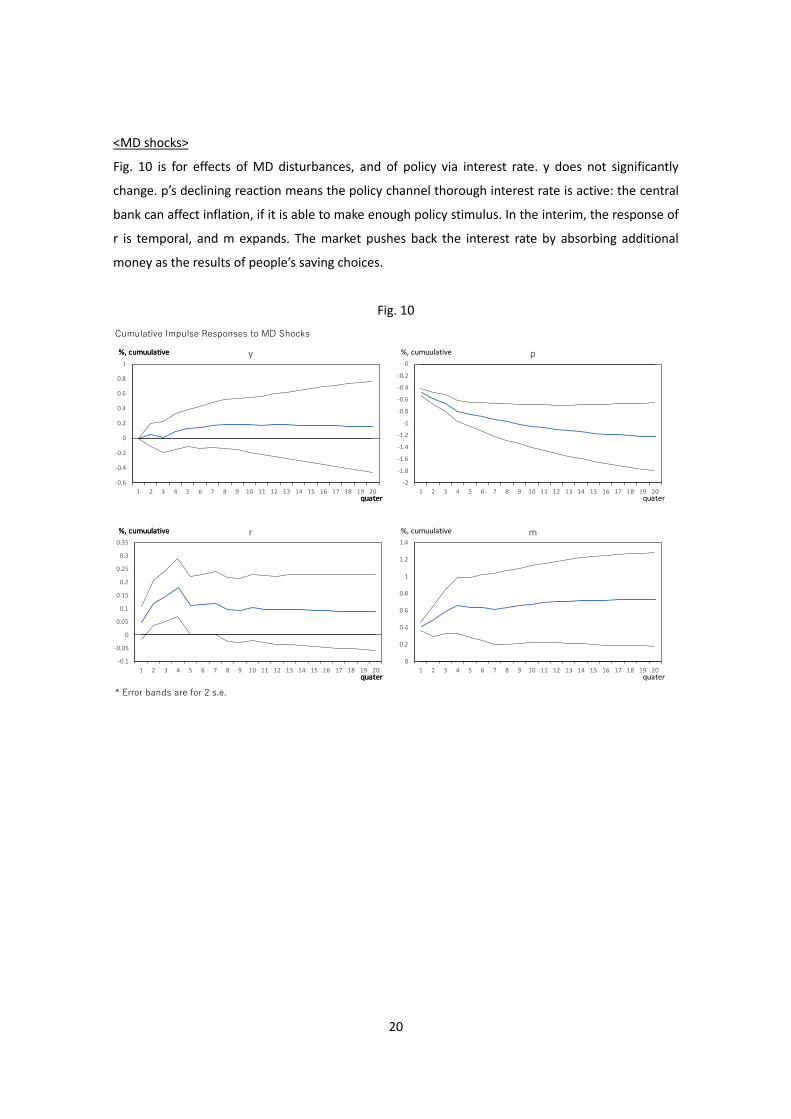
<MD shocks>
Fig. 10 is for effects of MD disturbances, and of policy via interest rate. y does not significantly
change. p’s declining reaction means the policy channel thorough interest rate is active: the central
bank can affect inflation, if it is able to make enough policy stimulus. In the interim, the response of
r is temporal, and m expands. The market pushes back the interest rate by absorbing additional
money as the results of people’s saving choices.
Fig. 10
Cumulative Impulse Responses to MD Shocks
* Error bands are for 2 s.e.
-0.6
-0.4
-0.2
0
0.2
0.4
0.6
0.8
1
1 2 3 4 5 6 7 8 9 10 11 12 13 14 15 16 17 18 19 20
y%, cumuulative
quater
%, cumuulative
quater
-0.1
-0.05
0
0.05
0.1
0.15
0.2
0.25
0.3
0.35
1 2 3 4 5 6 7 8 9 10 11 12 13 14 15 16 17 18 19 20
r%, cumuulative
quater
%, cumuulative
quater
0
0.2
0.4
0.6
0.8
1
1.2
1.4
1 2 3 4 5 6 7 8 9 10 11 12 13 14 15 16 17 18 19 20
m%, cumuulative
quater
-2
-1.8
-1.6
-1.4
-1.2
-1
-0.8
-0.6
-0.4
-0.2
0
1 2 3 4 5 6 7 8 9 10 11 12 13 14 15 16 17 18 19 20
p%, cumuulative
quater
21
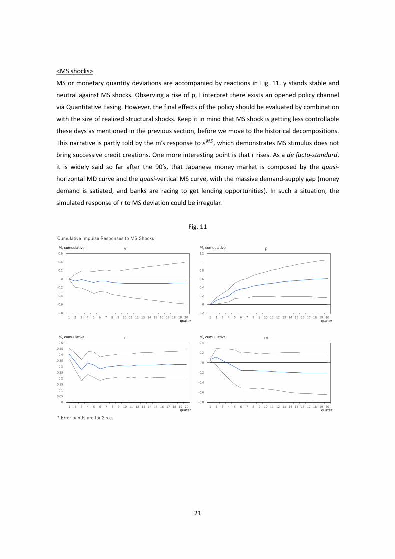
<MS shocks>
MS or monetary quantity deviations are accompanied by reactions in Fig. 11. y stands stable and
neutral against MS shocks. Observing a rise of p, I interpret there exists an opened policy channel
via Quantitative Easing. However, the final effects of the policy should be evaluated by combination
with the size of realized structural shocks. Keep it in mind that MS shock is getting less controllable
these days as mentioned in the previous section, before we move to the historical decompositions.
This narrative is partly told by the m’s response to 𝜀𝜀𝑀𝑀𝐴𝐴, which demonstrates MS stimulus does not
bring successive credit creations. One more interesting point is that r rises. As a de facto-standard,
it is widely said so far after the 90’s, that Japanese money market is composed by the quasi-
horizontal MD curve and the quasi-vertical MS curve, with the massive demand-supply gap (money
demand is satiated, and banks are racing to get lending opportunities). In such a situation, the
simulated response of r to MS deviation could be irregular.
Fig. 11
Cumulative Impulse Responses to MS Shocks
* Error bands are for 2 s.e.
-0.8
-0.6
-0.4
-0.2
0
0.2
0.4
0.6
1 2 3 4 5 6 7 8 9 10 11 12 13 14 15 16 17 18 19 20
y%, cumuulative
quater
0
0.05
0.1
0.15
0.2
0.25
0.3
0.35
0.4
0.45
0.5
1 2 3 4 5 6 7 8 9 10 11 12 13 14 15 16 17 18 19 20
r%, cumuulative
quater
-0.8
-0.6
-0.4
-0.2
0
0.2
0.4
1 2 3 4 5 6 7 8 9 10 11 12 13 14 15 16 17 18 19 20
m%, cumuulative
quater
-0.2
0
0.2
0.4
0.6
0.8
1
1.2
1 2 3 4 5 6 7 8 9 10 11 12 13 14 15 16 17 18 19 20
p%, cumuulative
quater
22
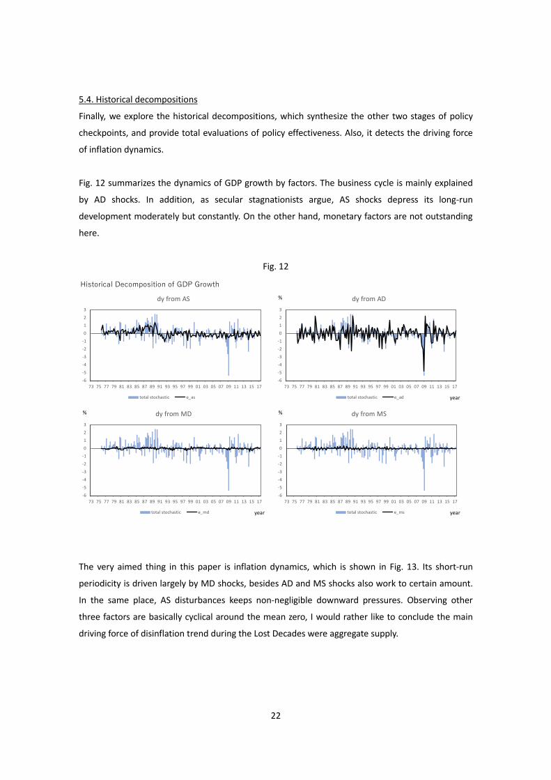
5.4. Historical decompositions
Finally, we explore the historical decompositions, which synthesize the other two stages of policy
checkpoints, and provide total evaluations of policy effectiveness. Also, it detects the driving force
of inflation dynamics.
Fig. 12 summarizes the dynamics of GDP growth by factors. The business cycle is mainly explained
by AD shocks. In addition, as secular stagnationists argue, AS shocks depress its long-run
development moderately but constantly. On the other hand, monetary factors are not outstanding
here.
Fig. 12
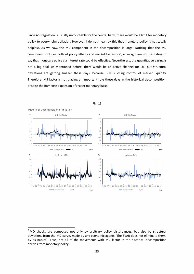
The very aimed thing in this paper is inflation dynamics, which is shown in Fig. 13. Its short-run
periodicity is driven largely by MD shocks, besides AD and MS shocks also work to certain amount.
In the same place, AS disturbances keeps non-negligible downward pressures. Observing other
three factors are basically cyclical around the mean zero, I would rather like to conclude the main
driving force of disinflation trend during the Lost Decades were aggregate supply.
Historical Decomposition of GDP Growth
-6
-5
-4
-3
-2
-1
0
1
2
3
73 75 77 79 81 83 85 87 89 91 93 95 97 99 01 03 05 07 09 11 13 15 17
dy from AS
total stochastic e_as zero
-6
-5
-4
-3
-2
-1
0
1
2
3
73 75 77 79 81 83 85 87 89 91 93 95 97 99 01 03 05 07 09 11 13 15 17
dy from AD
total stochastic e_ad
%
year
-6
-5
-4
-3
-2
-1
0
1
2
3
73 75 77 79 81 83 85 87 89 91 93 95 97 99 01 03 05 07 09 11 13 15 17
dy from MD
total stochastic e_md
%
year
-6
-5
-4
-3
-2
-1
0
1
2
3
73 75 77 79 81 83 85 87 89 91 93 95 97 99 01 03 05 07 09 11 13 15 17
dy from MS
total stochastic e_ms
%
year
23
Since AS stagnation is usually untouchable for the central bank, there would be a limit for monetary
policy to overwhelm deflation. However, I do not mean by this that monetary policy is not totally
helpless. As we saw, the MD component in the decomposition is large. Noticing that the MD
component includes both of policy effects and market behaviors7, anyway, I am not hesitating to
say that monetary policy via interest rate could be effective. Nevertheless, the quantitative easing is
not a big deal. As mentioned before, there would be an active channel for QE, but structural
deviations are getting smaller these days, because BOJ is losing control of market liquidity.
Therefore, MS factor is not playing an important role these days in the historical decomposition,
despite the immense expansion of recent monetary base.
Fig. 13
7 MD shocks are composed not only by arbitrary policy disturbances, but also by structural deviations from the MD curve, made by any economic agents (The SVAR does not eliminate them, by its nature). Thus, not all of the movements with MD factor in the historical decomposition derives from monetary policy.
Historical Decomposition of Inflation
-1.5
-1
-0.5
0
0.5
1
1.5
2
2.5
73 75 77 79 81 83 85 87 89 91 93 95 97 99 01 03 05 07 09 11 13 15 17
dp from AS
total stochastic e_as
%
year
-1.5
-1
-0.5
0
0.5
1
1.5
2
2.5
73 75 77 79 81 83 85 87 89 91 93 95 97 99 01 03 05 07 09 11 13 15 17
dp from AD
total stochastic e_ad
%
year
-1.5
-1
-0.5
0
0.5
1
1.5
2
2.5
73 75 77 79 81 83 85 87 89 91 93 95 97 99 01 03 05 07 09 11 13 15 17
dp from MD
total stochastic e_md
%
year
-1.5
-1
-0.5
0
0.5
1
1.5
2
2.5
73 75 77 79 81 83 85 87 89 91 93 95 97 99 01 03 05 07 09 11 13 15 17
dp from MS
total stochastic e_ms
%
year

24
6. Concluding Remark
In conclusion, to answer the two initial questions, 1) Japanese long-run deflation is mainly driven by
AS factor, and 2) Quantitative Easing is losing its effectiveness, whereas BOJ could still fight against
through via interest rate.
Note that the results above are from the mean estimation with long sample, so it should be
discounted that they are not specific results to the recent situations. Then, future effectiveness of
interest rate policy depends on conditions such as how strongly the ZLB will be bounding the
market. In addition, there would be side effects with today’s aggressive policy (for instance,
excessive low interest rate would distort the market functions), which I am not taking in the scope
here. Anyhow, after taking these into account, it would be better to reconsider the explosive
Quantitative Easing.
25
Appendix: Robustness Check
In this appendix, I check robustness of the results, by the following two alternative estimations. For
each trial, there are shown the figures for historical decompositions of inflation (because the
essence of the conclusions is summarized there). In each result, I can say that the qualitative
implications on inflation dynamics and policy effectiveness are unchanged.
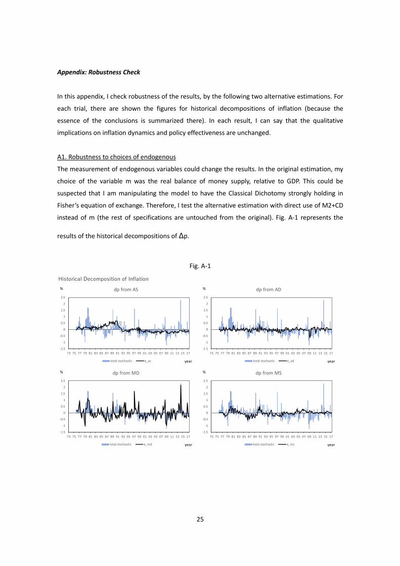
A1. Robustness to choices of endogenous
The measurement of endogenous variables could change the results. In the original estimation, my
choice of the variable m was the real balance of money supply, relative to GDP. This could be
suspected that I am manipulating the model to have the Classical Dichotomy strongly holding in
Fisher’s equation of exchange. Therefore, I test the alternative estimation with direct use of M2+CD
instead of m (the rest of specifications are untouched from the original). Fig. A-1 represents the
results of the historical decompositions of Δp.
Fig. A-1
Historical Decomposition of Inflation
-1.5
-1
-0.5
0
0.5
1
1.5
2
2.5
73 75 77 79 81 83 85 87 89 91 93 95 97 99 01 03 05 07 09 11 13 15 17
dp from AS
total stochastic e_as
%
year
-1.5
-1
-0.5
0
0.5
1
1.5
2
2.5
73 75 77 79 81 83 85 87 89 91 93 95 97 99 01 03 05 07 09 11 13 15 17
dp from AD
total stochastic e_ad
%
year
-1.5
-1
-0.5
0
0.5
1
1.5
2
2.5
73 75 77 79 81 83 85 87 89 91 93 95 97 99 01 03 05 07 09 11 13 15 17
dp from MD
total stochastic e_md
%
year
-1.5
-1
-0.5
0
0.5
1
1.5
2
2.5
73 75 77 79 81 83 85 87 89 91 93 95 97 99 01 03 05 07 09 11 13 15 17
dp from MS
total stochastic e_ms
%
year
26
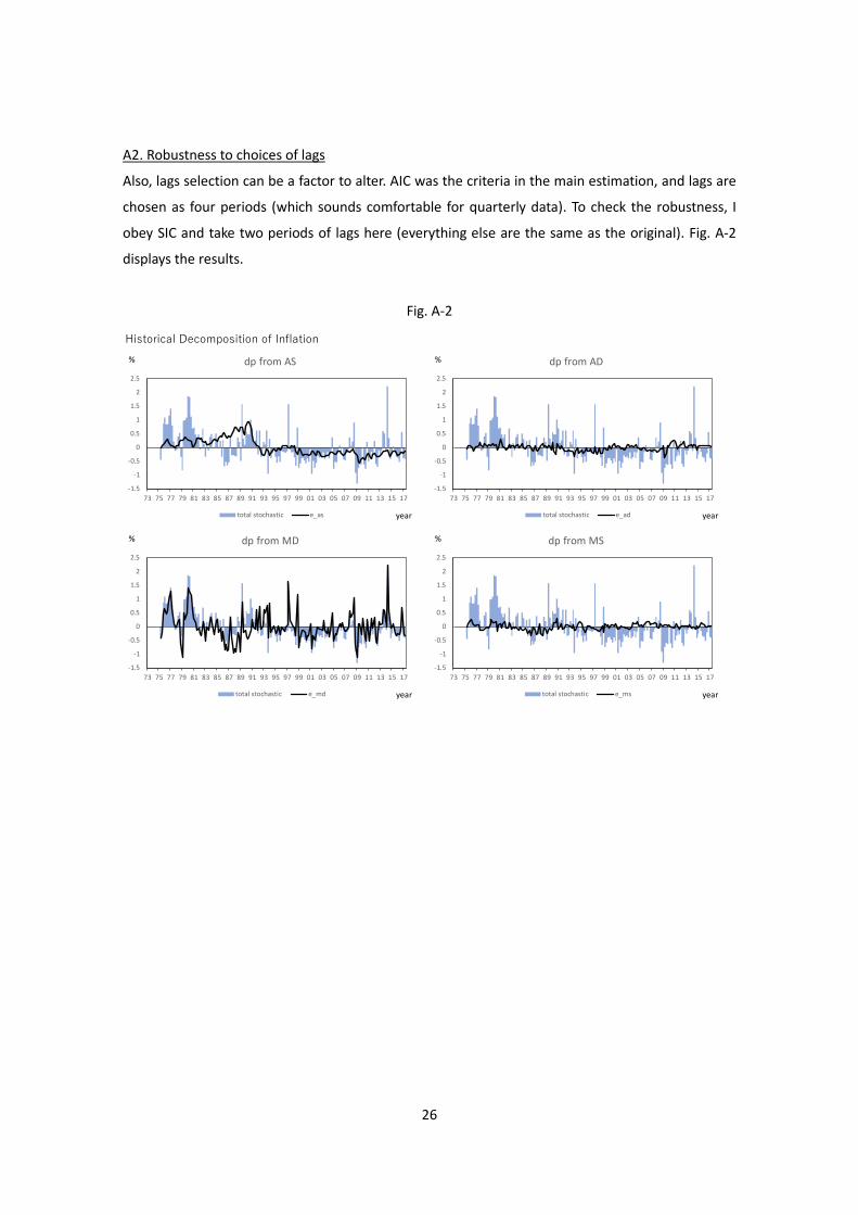
A2. Robustness to choices of lags
Also, lags selection can be a factor to alter. AIC was the criteria in the main estimation, and lags are
chosen as four periods (which sounds comfortable for quarterly data). To check the robustness, I
obey SIC and take two periods of lags here (everything else are the same as the original). Fig. A-2
displays the results.
Fig. A-2
Historical Decomposition of Inflation
-1.5
-1
-0.5
0
0.5
1
1.5
2
2.5
73 75 77 79 81 83 85 87 89 91 93 95 97 99 01 03 05 07 09 11 13 15 17
dp from AS
total stochastic e_as
%
year
-1.5
-1
-0.5
0
0.5
1
1.5
2
2.5
73 75 77 79 81 83 85 87 89 91 93 95 97 99 01 03 05 07 09 11 13 15 17
dp from AD
total stochastic e_ad
%
year
-1.5
-1
-0.5
0
0.5
1
1.5
2
2.5
73 75 77 79 81 83 85 87 89 91 93 95 97 99 01 03 05 07 09 11 13 15 17
dp from MD
total stochastic e_md
%
year
-1.5
-1
-0.5
0
0.5
1
1.5
2
2.5
73 75 77 79 81 83 85 87 89 91 93 95 97 99 01 03 05 07 09 11 13 15 17
dp from MS
total stochastic e_ms
%
year
27
References
Blanchard, O. J. and D. Quah (1989), “The dynamic effects of aggregate demand and supply
disturbances”, The American Economic Review, 82(4), 901-921.
―――― (1993), “The Dynamic effects of aggregate demand and supply disturbances: Reply”, The
American Economic Review, 83(3), 653-658.
Dickey, D. A. and W. A. Fuller (1979), “Distribution of the estimators for autoregressive time series
with a unit root”, Journal of the American Statistical Association, 74, 427-431.
Eggertsson, G. B. (2010), “What fiscal policy is effective at zero interest rates?”, NBER
Macroeconomics Annual, University of Chicago Press, 25, 59-112.
Faust, J. and M. Leeper (1997), “When do long-run identification restrictions give reliable results?”,
Journal of Business & Economic Statistics, 15(3), 345-353.
Gali, J. (1992), “How well does the IS-LM model fit postwar U.S. data?”, Quarterly Journal of
Economics, May., 709-738.
Gerlach, S. and F. Smets (1995), “The monetary transmission mechanism: Evidence from the G-7
countries”, BIS working paper, No. 26.
Hyndman, R. J., A. B. Koehler, R. D. Snyder, and S. Grose (2002), “A state space framework for
automatic forecasting using exponential smoothing methods,” International Journal of Forecasting,
18, 439-454.
Johansen, S. and K. Juselius (1990), “Maximum likelihood estimation and inferences on
cointegration —with applications to the demand for money”, Oxford Bulletin of Economics and
Statistics, 52, 169-210.
Kwiatkowski, D., P. C. B. Phillips, P. Schmidt and Y. Shin (1992), “Testing the null hypothesis of
stationary against the alternative of a unit root”, Journal of Econometrics, 54, 159-178.
Lippi, M., and L. Reichlin (1993), “The dynamic effects of aggregate demand and supply
28
disturbances: Comment”, The American Economic Review, 83(3), 644-652.
Ljung, G. M. and G. E. P. Box (1978), "On a measure of a lack of fit in time series models",
Biometrika, 65(2), 297-303.
MacKinnon, J. G. (1996), “Numerical distribution functions for unit root and cointegration tests”,
Journal of Applied Econometrics, 11, 601-618.
MacKinnon, J. G., A. A. Haug, and L. Michelis (1999), “Numerical distribution functions of likelihood
ratio tests for cointegration”, Journal of Applied Econometrics, 14, 563-577.
Mio, H. (2002), “Identifying aggregate demand and aggregate supply components of inflation rate:
A structural vector autoregression analysis for Japan”, Monetary and Economic Studies, 20(1), 33-
56.
Schenkelberg, H. and S. Watzka (2013), “Real effects of quantitative easing at the zero lower bound:
Structural VAR-based evidence from Japan”, Journal of International Money and Finance, 33, 327-
357.
Shapiro, M. D., and M. W. Watson (1988), “Sources of business cycle fluctuations”, NBER
Macroeconomic Annual, MIT Press, 3, 111-156.
Stock, J. H., and M. W. Watson (2001), “Vector autoregressions”, The Journal of Economic
Perspectives, 15(4), 101-115.