Sources of Comparative Advantage in Polluting Industries∗

Fernando Broner Paula Bustos Vasco M. Carvalho†

February 2012

Abstract

We study the determinants of comparative advantage in polluting industries by analyz-

ing how country and industry characteristics interact to determine trade flows. We find that

countries with weaker environmental regulation export relatively more in polluting industries,

consistent with a pollution haven effect. Furthermore, this effect is quantitatively important

and comparable in magnitude to traditional sources of comparative advantage such as skill and

capital abundance. However, these estimates cannot be interpreted as causal: countries with a

comparative advantage in polluting industries could have stronger lobbies against environmental

regulation. Thus we propose an instrument for environmental regulation based on exogenous

meteorological determinants of pollution dispersion identified by the atmospheric pollution sci-

ence literature. We find that the pollution heaven effect is indeed causal and stronger than

suggested by OLS estimates.

∗We thank Bruno Caprettini for superb research assistance. We received valuable comments from David Atkin,

Gene Grossman, Elhanan Helpman, Wolfgang Keller, Giacomo Ponzetto, Daniel Sturm and participants at pre-

sentations held at Central European University, CREI, UPF, ERWIT, and Princeton IES Summer Workshop. We

acknowledge financial support from the Fundación Ramón Areces.†CREI, Universitat Pompeu Fabra and Barcelona GSE (www.crei.cat).

1 Introduction

What are the sources of comparative advantage in polluting industries? This is an old question

in the literature on international trade and the environment. Theory provides a straightforward

answer. Everything else equal, countries with lax environmental regulation should have a compar-

ative advantage in polluting industries. This result is known as the pollution haven effect. Despite

its theoretical appeal, there is still no consensus in the empirical literature about its economic

relevance.

To address this question, we analyze how country and industry characteristics interact to deter-

mine comparative advantage in polluting industries. We find that countries with laxer environmen-

tal regulation export relatively more in polluting industries. This effect is quantitatively important

and comparable in magnitude to traditional sources of comparative advantage such as skill and

capital abundance. However, these estimates cannot be interpreted as causal: countries with a

comparative advantage in polluting industries could have stronger lobbies against environmental

regulation. Thus we propose an instrument for environmental regulation based on exogenous me-

teorological determinants of pollution dispersion identified by the atmospheric pollution science

literature. We find that the pollution heaven effect is indeed causal and stronger than suggested

by OLS estimates.

To guide the empirical work, we begin by presenting a simple model that analyzes the effects

of environmental policy on the patterns of international trade. As is standard in the literature

on trade and the environment [Copeland and Taylor (2003)], we treat pollution as another factor

of production, whose relative supply is determined by environmental policy. We illustrate how

countries with lax environmental regulation tend to have a comparative advantage in polluting

industries. The model emphasizes the endogenous determination of environmental regulation. In

particular, environmental policy depends on technology and income and also on how costly pollution

is in each country. The model shows that countries in which pollution is less costly in welfare terms

will tend to adopt laxer environmental policy. This result is crucial to motivate our choice of

instrument for environmental policy.

Turning to our empirical strategy, we extend the standard cross-country, cross-industry method-

ology to study the determinants of comparative advantage proposed by Romalis (2004).1 Specif-

ically, we treat pollution intensity as a technological characteristic of industries, like capital and

skill intensity. At the same time, we treat environmental regulation as a characteristic of countries,

like capital and skill abundance. We ask whether countries with laxer environmental regulation

1This approach has been used to study a variety of sources of comparative advantage. See, for example, Levchenko

(2007), Nunn (2007), Manova (2008), Costinot (2009), Chor (2010), and Cuñat and Melitz (forthcoming).

1

have a comparative advantage in polluting industries, while controlling for other determinants of

comparative advantage. An advantage of this procedure is that it allows us to study the sources

of comparative advantage in polluting industries more broadly than existing studies, as we do not

focus on particular industries or trading partners.

We find evidence consistent with the pollution haven effect. That is, we show that countries

with laxer environmental regulation tend to export relatively more in polluting industries. Further-

more, we find that these effects are quantitatively important. As an example, consider the following

thought experiment. Take South Africa, a country with average air pollution regulation stringency

in our sample. Now consider the effects of South Africa adopting a more stringent environmental

policy, say to the level of France which is one standard deviation above the mean of cross-country

regulatory stringency. We find that South Africa’s exports to the U.S. in pollution-intensive indus-

tries would decrease significantly. For example, relative to South Africa’s average market share in

the U.S., the share of its exports in steel products manufacturing, which is one standard deviation

more pollution intensive than the typical industry, would decrease by 10 percent. Moreover, this

effect is comparable in magnitude to more traditional determinants of comparative advantage. In

particular, in an analogous experiment, increasing skill (capital) abundance would yield an increase

in the relative shares of skill (capital) intensive industries of 7 percent (3 percent).

An important concern regarding the interpretation of the results outlined above is the direction

of causality. For example, in countries in which polluting industries are more important they might

lobby more successfully to prevent the enactment of strong environmental regulations. This would

imply that comparative advantage in polluting industries causes laxer environmental policy, leading

to a positive bias. On the other hand, reverse causality could lead to a negative bias if in the face

of a heavily polluted environment citizens successfully push for stricter regulation.2 To address

this concern we need an instrument for environmental regulation. That is, a source of variation in

environmental regulation that is not determined by comparative advantage in polluting industries

(exogenous) and does not affect comparative advantage through other channels (exclusion restric-

tion). To find such an instrument we turn to the large and established literature on the determinants

of atmospheric pollution. This literature has identified a number of meteorological variables that

determine the speed of dispersion of pollutants. As suggested by the model, our hypothesis is that

meteorological conditions that facilitate the dispersion of pollutants in the atmosphere are likely

to lead to a lower marginal cost of emissions for a given level of pollution and thus to laxer air

pollution regulation.

2For a more thorough discussion of potential problems of reverse causality see Ederington and Minier (2003) and

Levinson and Taylor (2008).

2

Our measure of the speed of air pollution dispersion is the "ventilation coefficient." This coef-

ficient is the product of two exogenous meteorological determinants of pollution dispersion in the

atmosphere: wind speed, which determines horizontal dispersion of pollution, and mixing height,

which determines the height within which pollutants disperse in the atmosphere. The ventilation

coefficient is the main determinant of pollution dispersion according to the standard Box model of

atmospheric pollution. This model thus provides us with a simple metric to assess and compare

the potential for pollution dispersion across countries: given two countries with the same level of

emissions the country with the higher ventilation coefficient will have lower pollution concentration.

The instrumental variable estimates of the effect of environmental regulation on comparative

advantage in polluting industries are around 80% higher than OLS estimates. This finding points

towards two sources of bias in the OLS estimates. First, OLS estimates can be biased downwards

if countries with a comparative advantage in polluting industries face stronger demand from their

citizens to address air pollution problems and thus enact stricter regulation. Second, our measure

of environmental regulation captures a single dimension of policy, thus OLS estimates might be

downward biased due to measurement error.

We contribute to a rich literature studying the role of environmental regulation on comparative

advantage. Early studies focused on establishing cross-country trends. Between 1960 and the

early 1990’s pollution-intensive output as a percentage of total manufacturing fell in the OECD

and increased in the developing world. In addition, those periods of rapid increase in net exports

of pollution-intensive products from developing countries coincided with periods of rapid increase

in the cost of pollution abatement in OECD countries.3 Although consistent with the pollution

haven effect, these trends could also be accounted for by other mechanisms. For example, capital

accumulation in developing countries could lead to an increasing comparative advantage in capital-

intensive goods, which only happen to be polluting.

More recent studies have sought to establish a direct link between environmental regulation,

the location of polluting industries, and the resulting pattern of trade. These papers emphasize the

cross-industry variation in U.S. environmental regulation and use pollution abatement costs as a

proxy for regulation at the industry level. The first studies did not find strong effects of abatement

costs on trade flows [Grossman and Krueger (1993)].4 In contrast, Levinson and Taylor (2008) find

that industries whose abatement costs increased more experienced larger increases in imports when

3See Jaffe et al. (1995), and Mani and Wheeler (1999). These trends have accelerated since the early 1990s. For

example, sulfur dioxide emissions have been reduced by half in both the US and Europe since the early 1990s (see

United States Environmental Protection Agency Clearinghouse for Inventories and Emissions Factors and European

Environmental Agency). On the other hand, sulfur dioxide emissions in China are estimated to have increased by

50% between 2000 and 2006 (see Lu et al., 2010).4For a survey of the literature, see Copeland and Taylor (2004).

3

instrumenting for pollution abatement costs.5 However Ederington, Levinson and Minier (2005)

find that increases in abatement costs increase imports only in footloose industries, which happen

to be the least polluting ones. In contrast, we find that differences in environmental regulation

across countries have strong effects on exports of polluting industries.

Finally, let us note that we find that countries weak environmental regulation have a compar-

ative advantage in polluting industries even without controlling for other sources of comparative

advantage. This result, referred to in the literature as the pollution haven hypothesis, is usually

considered to be stronger than the pollution haven effect.6 As countries with weak environmental

regulation are usually capital scarce and capital intensive sectors tend to be polluting, there is

potentially an effect going in the opposite direction: capital abundant countries could specialize

in polluting industries. Our evidence suggests that the magnitude of the pollution heaven effect

is large enough to dominate this potentially countervailing effect.7 The evidence in this paper

also helps reconcile the effects of environmental regulation on international trade flows, tradition-

ally viewed as weak, with a large body of evidence documenting a strong effect of environmental

regulation on plant location and FDI flows.8

The paper is organized as follows. Section 2 presents the theoretical model. Section 3 describes

the data. Section 4 presents our OLS empirical results. Section 5 describes our meteorological

instrument. Section 6 presents the instrumental variable results. Section 7 concludes.

2 Pollution and environmental regulation in a standard model of

trade

In this section we present a simple model that illustrates how environmental policy and income

affects comparative advantage in polluting industries. It also shows how ventilation potential and

income, in turn, affect environmental policy.

5As Levinson and Taylor (2008) point out, the use of pollution abatement costs presents a number problems. In

particular, compositional effects within industries might make pollution abatement costs a poor proxy for policy.

Also, environmental regulation at the industry level may be endogenous due to political economy factors. These

problems can result in a variety of biases that may explain the negative results. Indeed, when Levinson and Taylor

(2008) account for the endogeneity of environmental regulation they find a positive effect of changes in pollution

abatement costs between 1977 and 1986 on changes in U.S. imports from Mexico and Canada. See also Ederington

and Minier (2003).6For a more detailed discussion of the pollution haven hypothesis and the pollution haven effect see Copeland and

Taylor (2004).7Still, it is important to emphasize that even the pollution haven hypothesis does not imply that international trade

with countries with weak environmental regulation should increase global pollution. In particular, several papers have

argued that trade liberalization can lead to growth which in turn might induce countries to enact more stringent

environmental regulation or adopt cleaner technologies [Grossman and Krueger (1993), Antweiler, Copeland, and

Taylor (2001), and Levinson (2009)].8See for example Becker and Henderson (2000), Greenstone (2002), Keller and Levinson (2002) and List et al.

(2003).

4

2.1 Setup

There are many small countries, indexed by ∈ . Labor is the only factor of production. There is

a mass one of residents in every country, each endowed with units of labor. There are two goods,

one clean and one dirty, both of which are tradable. Production of the clean good requires labor

and does not pollute. Labor productivity in country is , so that

= · ,

where is production of the clean good and is labor allocated to the clean industry. Produc-

tion of the dirty good does not require labor but is polluting. In particular, each unit of the dirty

good produces − units of pollution, so that

= · ,

where is production of the dirty good and is pollution produced in the dirty industry.

The parameter ∈ [0 1] captures the extent to which countries with higher productivity also haveaccess to better abatement technologies. Factor market clearing implies that

= · = · and = · =

· ,

where is total pollution produced in country .9

Utility is increasing in consumption of the clean and dirty goods and decreasing in pollution.

We assume that pollution only affects utility in the country where it is produced. In particular,

utility in country is

³ ·

´−

¡ ·

¢, (1)

where + = 1, 0 0, 00 0, 0 0, 00 0, and measures how costly in utility

terms is pollution in country . The parameter is inversely related to the ventilation potential

of country . In particular, meteorological conditions that facilitate the dispersal of pollutants will

be associated with a low .

Producing the dirty good is associated with a negative local externality. Countries address

this externality by imposing pollution limits.10 In particular, in each country there is a cap on

9Our treatment of pollution as another factor in the production process is standard in the literature on trade and

the environment. See Copeland and Taylor (2003) for a textbook analysis.10 In the literature environmental policy is often modeled as a pollution tax. In this model pollution taxes would

have effects that are too extreme. The reason is that countries would produce either zero or an infinite amount of

the dirty good depending on whether · is lower or higher than the tax. In reality, environmental policy often

5

pollution,

≤ , (2)

that is implemented by distributing pollution rights to each resident of . Each country chooses

its optimal pollution limit taking those of the other countries as given.11

2.2 Equilibrium

To obtain the equilibrium we proceed in two steps going backwards. First, we solve the model for

a given pattern of pollution limits for ∈ . Second, we find the equilibrium pollution limits,

which are chosen optimally by each country.

The first step is very simple. Given pollution limits, the model is isomorphic to a two-good,

two-factor model in which pollution is a second factor of production as opposed to a by-product.12

Since the price of the dirty good is positive, Constraint (2) is binding and production is given by

= · and = · for ∈ . (3)

Let and be the prices of the clean and dirty goods respectively. For any and , country

produces · units of the clean good and · units of the dirty good. Given Cobb-Douglas

preferences, consumption is given by

= ·

³ · · + ·

·

´

for ∈ { } . (4)

Integrating this equation over all countries for the clean good and imposing the market clearing

conditionR∈ =

R∈ · , we obtain the relative price of the dirty good

=

·R∈ ·

·R∈

·

. (5)

Normalizing prices so that the price of the “composite good” ·

is one, we obtain

= ·ÃR

∈ · R

∈ ·

!

and = ·Ã R

∈ · R∈

·

!

. (6)

takes the form of quantity limits as countries impose restrictions on the location and size of different industries. Also,

policy often responds more strongly when the concentration of pollutants in the air reaches certain limits.11The equilibrium in this model is efficient even though countries are small because the externalities are local. This

would not be the case for pollutants associated with global externalities, most notably green house gases.12The second term in Equation (1) can be disregarded in this step as, given pollution limits, it is equal to the

constant ·

.

6

With this normalization, welfare is given by

¡¡

¢¢− ¡ ·

¢for ∈ , (7)

where ¡

¢ ≡ · · + · · is income. Equations (3), (4), (6), and (7) describe the

equilibrium for a given pattern of pollution limits for ∈ .

Since countries are small, we can analyze the effects of changes in country characteristics taking

as given goods prices. In particular, consider an increase in pollution limits . Equations (3) and

(4) show that is unaffected and , , and increase. As a result, exports of the clean

good, − , decrease and exports of the dirty good, − , increase. The following result

follows.

Result 1. An increase in pollution limits leads to more comparative advantage in the dirty good.

We now turn to the determination of pollution limits for ∈ . Country chooses to

maximize its welfare in Equation (7), taking as given goods prices and . The optimum ∗ is

determined implicitly by the first order condition

0 = · · 0

¡¡∗¢¢− · 0

¡ · ∗

¢. (8)

This conditions shows that countries trade off the increase in income associated with an additional

unit of pollution with the utility cost of the additional pollution.

How does ∗ depend on pollution cost ? Once again, since countries are small we can analyze

the effect of taking as given goods prices. Take the total derivative of Equation (8) with respect

to and rearrange to obtain

∗

=− 0

³ · ∗

´− · ∗ · 00

³ · ∗

´2 · 00

³ · ∗

´− 2 ·2· · 00

³

³∗´´ .

Given the properties of (·) and (·), it is clear that the numerator is negative and the denominatoris positive. The following result follows.

Result 2. An increase in pollution cost leads to lower pollution limits ,

∗

0. (9)

The intuition is straightforward. A higher means that the country is willing to accept less

7

consumption of goods in exchange for lower pollution levels, leading to more stringent environmental

standards.

How does ∗ depend on productivity ? In principle, this effect is ambiguous because there

are two opposing effects. On the one hand, a higher has an income effect that leads to lower

pollution limits, as the country wants to increase its consumption of “clean air.” On the other hand,

a higher has a substitution effect that leads to higher pollution limits since producing the dirty

good becomes less polluting. The latter effect, of course, depends on . In the appendix we show

the following result.

Result 3. An increase in productivity has an ambiguous effect on pollution limits . However,

the effect is unambiguously negative,∗

0, (10)

if either (i) = 0, or (ii) the coefficient of relative risk aversion − · 00 ()/ 0 () 1.

The first condition is due to the fact that the substitution effect disappears if = 0. The second

condition is due to the fact that, even if = 1, the income effect dominates the substitution effect

when the coefficient of relative risk aversion is greater than 1.

The analysis in this section has clear empirical predictions. First, conditional on other country

characteristics, countries with less stringent environmental policy have a comparative advantage in

polluting industries. Second, environmental policy is less stringent in countries with high ventilation

potential. In addition, environmental policy is likely to be more stringent in richer countries.

3 Data

In this section we introduce measures of an industry’s air pollution intensity and the strictness of

a country’s air pollution regulations. We describe each of these measures in detail below and then

combine them with U.S. bilateral trade flows to take a first look at the evidence: is cross-country

variation in the strictness of air pollution regulations an important determinant of comparative

advantage in polluting industries?

The remaining sources of data used in the paper are standard in the literature. The data on

bilateral trade flows with the U.S. is from Feenstra, Romalis and Schott (2002), updated till 2006.

We source data on cross-country stocks of human capital and physical capital from Hall and Jones

(1998). Data on skill and capital intensity at the industry level is available for the manufacturing

sector only and is sourced from Bartelsman and Gray’s (1996) NBER-CES manufacturing data,

updated to 2005.

8

3.1 A measure of air pollution intensity

Our measure of air pollution intensity at the industry level is drawn from data compiled by the U.S.

Environmental Protection Agency’s (EPA) in their Trade and Environmental Assessment Model

(TEAM).13 TEAM’s air emissions baseline data is based on the EPA’s 2002 National Emissions

Inventory.14 From this data set, we obtain - for a host of air pollutants - the total amount of

air pollution emitted by 4-digit NAICS industries in the US in 2002. Throughout, we focus our

analysis on industry level emissions data of three common air pollutants: Carbon Monoxide (CO),

Nitrogen Oxides (NOx) and Sulfur Dioxide (SO2).

Given information on the value of sales in each industry we can then compute the corresponding

pollution emission intensity (per dollar of sales in a given industry). In total, we have pollution

intensity data for 86 manufacturing industries.15 Within manufacturing, metal manufacturing,

mineral (non-metallic) products manufacturing, paper manufacturing, chemical manufacturing and

petroleum and coal products make it to the top of the list in every pollutant ranking displayed in

Table 1.

Our list of most pollution intensive manufacturing industries is broadly consistent with the

ranking "dirty industries" in Mani and Wheeler (1999) which uses an alternative indicator of

pollution intensity based on the Industrial Pollution Projection System (IPSS) data set assembled

by the World Bank.16 17 More generally, as Hettige et al (1995) had noted for IPSS data, there is

extreme sectorial variation in emission factors, the distribution being very fat tailed. As an example,

the least pollution intensive manufacturing sector in Carbon Monoxide - Tobacco manufacturing-

is 24 times less polluting than the most CO intensive industry within manufacturing, Alumina and

aluminum production. The upshot of this is that the ten most pollution intensive manufacturing

sectors account for a significant amount of total manufacturing air pollution emissions in every

13This data is assembled by the EPA and Abt Associates. See Abt Associates (2009) for a complete description.14Specifically, for each pollutant, we sum across point (i.e. those deriving from large polluting facilities), area and

mobile source measurements at the national level.15Given our focus on manufacturing industries we do not exploit information on 180 service sector industries and

28 agriculture and mining industries.16The IPPS data also gives pollution intensity per sector across a range of pollutants. However this data refers to

1987 measurements. Thus our EPA-TEAM data is based on a newer vintage data. Furthermore, as Abt Associates

(2009) note, the data used in developing the IPPS pollutant output intensity coefficient, and the 1987 Toxic Release

Inventory (TRI) database in particular, "have been the subject of substantial concerns regarding their reliability.

This [1987] was the first year the TRI data were self-reported by facility. A 1990 EPA report found that 16 percent

of releases reported in the 1987 database were off by more than a factor of ten, and 23 percent were off by a factor

of two."17At this degree of sectoral disaggregation, it is difficult to find comparable data for other countries. Still, Cole et al

(2004) and Dean and Lovely (2008), when reporting 3-digit ISIC manufacturing pollution intensities for, respectively,

the UK during the 1990s and China in 1995 and 2004, single out the same highly polluting industries as we do here:

metal manufacturing, non-metallic mineral products, coke and petroleum and paper manufacturing. Reliable data at

this more aggregated level is available for at least a handful more of European countries and Canada. In the future

we plan to conduct a more systematic cross-country comparison of pollution intensity measures at the industry level.

9

pollutant, ranging from 38% for CO to 66% in SO2. Further, despite differences in the exact

ordering of sectors across pollutant categories, computing a rank correlation reveals a high average

correlation: highly pollution intensive industries in a given pollutant tend to be pollution intensive

in all pollutants (see Table 2). Table 3 reports the correlation of our measures of pollution intensity

and industry level factor intensities of production (skill and capital intensity). Across all pollutants,

pollution intensive industries tend to be capital intensive and unskilled intensive18.

3.2 A measure of air pollution regulation

Our measure of air pollution regulation is grams of lead content per liter of gasoline, a standard

measure of environmental stringency and previously used by, for example, Hilton and Levinson

(1998), Damania, List and Frederiksson (2003) and Cole, Elliot and Fredriksson (2006).

As Hilton and Levinson (1998) and Lovei (1998) discuss, lead emissions are one of the most

toxic substances to which populations around the world have been exposed to, posing severe health

problems ranging from cardiovascular diseases to significant reductions in the I.Q. of children ex-

posed to it. As a result, both national environmental agencies and international organizations have

targeted reduction in lead emissions. Lead is defined by the E.P.A. as a criteria air pollutant (since

1976) and both the World Bank and the United Nations Environment Program have been actively

involved in supporting national environmental policies that address lead pollution.

The largest source of lead exposure has traditionally been tail-pipe emissions from vehicles

fueled by leaded fuel. As a result, policies targeting lead pollution in the atmosphere have taken

the form of legislation on the lead content of gasoline. Thus, we source cross-country data on the

average lead content (in grams) per liter of gasoline from the World Bank (Lovei, 1998) which in

turn collects data from industry and consulting sources, World Bank reports and through direct

contact of government officials.19 From this, we obtain lead content data for 101 countries in 1996.

Our policy measure ranges from 0 - reflecting a ban on leaded gasoline in countries like Sweden or

Denmark - to 0.85 grams per liter of gasoline in Venezuela. A list of the ten least and ten most

stringent regulation countries according to this measure is provided in Table 4.

While admittedly narrow and applying primarily to the transportation sector, lead content per

gallon of gasoline is, to the best of our knowledge, the only actual air pollution regulation measure

18The positive correlation between pollution intensive and capital intensive industries is again in accordance with

the discussion of Mani and Wheeler (1999) for the IPSS dataset. See also Antweiler et al (2001).19While the extant literature as extensively used the lead content policy measure, the source of our lead content

data is novel. The literature has traditionally sourced the data from Associated Octel Ltd., the main commercial

producer of ethyl lead compounds up until recently. The World Bank technical report from which we source our data

(Lovei, 1998) cross-checks and supplements Octel’s data with a number of industry publications, World Bank sources

and through contacts with government officials.

10

available for a broad cross-section of countries. Further, as Damania et al (2003) discuss, this

variable correlates well with other proxies for the environmental stance of a country such as the

environmental stringency index put forth by Dasgupta et al (2001), public expenditure on environ-

mental R&D as a proportion of GDP or per capita membership of environmental organizations.

Our lead content measure is also negatively correlated with other traditional determinants of com-

parative advantage like capital and skill abundance20. This is as expected and reflects the fact

that richer countries have tended to spearhead efforts in addressing atmospheric lead pollution.

Thus, the correlation of grams of lead per liter of gasoline with log income per capita is −063 andsignificant at the 1% level. Still, as Lovei (1998) notes, governmental policies in several middle

and low income countries have also contributed to stringent policy being enacted in parts of the

developing world. This is the case of Bolivia or Thailand for example. This suggests that our

measure captures actual policy stringency and not simply the income of a country.

4 Determinants of Comparative Advantage in Polluting Goods

In this section we investigate whether lax environmental regulation can be a source of comparative

advantage in polluting goods. Anticipating the more detailed empirical analysis below, and as a

first look at the raw data, we ask whether the share of exports in pollution intensive industries is

larger for countries with weak air pollution regulations. To do this, we divide the sample into weak

versus strict air pollution regulation countries, defined as those with a measure of lead content

of gasoline, respectively, above and below the sample median. Similarly, we group industries into

those that are pollution intensive and those that are not. We define an industry to be pollution

intensive in a given pollutant if the corresponding if is in the top quartile of the distribution of total

pollution intensities for that pollutant. We find that, for weak regulation countries, 51 percent of

their manufacturing exports to the US are in NOx intensive industries while for strict air pollution

regulation counties only 28 percent of exports are in NOx intensive industries. The pattern repeats

itself for SO2 (48 versus 29 percent respectively) and CO (51 versus 31 percent respectively). Thus,

countries with weak air pollution regulations tend to export relatively more in pollution intensive

industries to the US.

Next, we conduct a more systematic analysis of the effects of environmental regulation on

exports of polluting goods. For this purpose, we incorporate environmental regulation as a country

characteristic and pollution intensity as an industry characteristic in a standard cross-country

cross-industry trade equation. In our model, regulation is implemented as a quantity restriction

20The correlation is −064 for capital abundance and −069 for skill abundance. Both are significant at the 1%level.

11

and it thus immediately admits a factor abundance interpretation. We thus treat environmental

regulation in the same way that we treat capital and skill abundance. The model also illustrates

how pollution can be interpreted as another input in production. We thus treat pollution intensity

in the same way that we treat capital and skill intensity.21

Our empirical specification takes the form

= 1 × + 2 × + 3 × + + + , (11)

where are country ´s relative import shares into the U.S. in industry , described in further

detail below; is a measure of the laxity of air pollution regulation in country ; is a measure

of the pollution intensity of industry ; and denote country ´s endowments of capital and

human capital; and are industry ´s capital and skill intensity; and are country and

industry fixed effects.22 Result (1) in Section 2, namely that a country with laxer environmental

regulation should export relatively more in polluting industries, would correspond to finding 1 1.

Our dependent variable, country ´s relative import shares () into the U.S., is defined as

country ´s trade share in sector divided by the average share of country in U.S. imports. This

normalization, suggested by Levchenko (2007), aims at making trade shares comparable across

countries by accounting for heterogeneity in country size and the closeness of the trade relationship

with the U.S. Alternatively, we could use a log-transformation of imports but this has the disad-

vantage of dropping the observations with zero trade, around one third of the total. We thus prefer

the specification in shares. Still, we obtain similar coefficient estimates both in terms of magnitude

and statistical significance when using the log of imports as our dependent variable, as we report

in Appendix 3.

For industry factor intensities, we use U.S. factor shares in value added. Since there is no com-

parable measure of pollution share in value added, we use the quantity of pollution emitted by each

industry divided by the value added of that industry in the U.S., i.e. =

±¡ ·

¢.

Under the assumption that all industries face the same effective price of pollution , this proce-

dure does not lead to biases in the estimation of Equation (11) because the use of amounts to

dividing the pollution share by a constant. Overall, this specification is correct if, as we assumed

in the model, differences across countries in technology and environmental policy do not affect the

relative pollution intensities of industries.

21Under some conditions, these interpretations are also appropriate in models in which regulation is implemented

as a pollution tax. See Copeland and Taylor (2003) for details.22This specification is an extension of the one used by Romalis (2004). Similar extensions have been used to explore

a variety of sources of comparative advantage by Levchenko (2007), Nunn (2007), Manova (2008), Costinot (2009),

Chor (2010), and Cuñat and Melitz (forthcoming).

12

4.1 Baseline Results

As measures of pollution intensity we use the simple average of pollution emitted per unit of output

for three air pollutants sulfur dioxide (SO2 ), nitrogen oxides (NOx ) and carbon monoxide (CO).

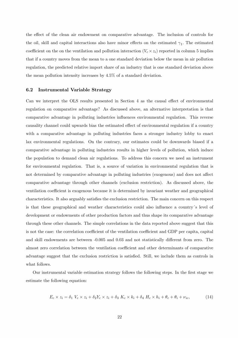
Table 5 reports estimation of Equation (11) for the average pollution intensity measure and also for

each of the three air pollutants separately, without controlling for capital and skill interactions. The

first row reports the estimate of 1 for the interaction of pollution intensity of the industry with

the lax air pollution regulation measure. The remaining columns report the analogous estimation

for the rest of the pollutants. The estimated 1 coefficient on the air pollution regulation and

air pollution intensity interaction ( × ) are positive and statistically significant at 1 percent

for each pollutant and the pollution intensity index. The estimated coefficient on the pollution

interaction ( × ) reported in column 1 implies that if a country moves from the mean to a

one standard deviation below the mean in air pollution regulation, the predicted relative import

share of an industry that is one standard deviation above the mean pollution intensity increases

by 6.24% of a standard deviation. In addition, their effects are of a similar magnitude.23 Thus,

to simplify the exposition, in what follows we only report estimates for the air pollution intensity

index. Like Table 5, all subsequent tables report robust standard errors below coefficient estimates.

To address potential correlation in errors across industries or countries, we show in Appendix 3, that

the estimated coefficients are also statistically significant when clustering errors across countries,

industries and both countries and industries.

Estimation of Equation (11) with controls for factor endowments and other determinants of

comparative advantage is reported in Table 6. Note that as measures of capital and skill endowments

are only available for a subset of countries, the sample is smaller than in Table 5. Columns 1 and

2 show that adding controls for capital and skill interactions ( × and × ) does not

significantly affect the estimated coefficients, which suggests that the environmental regulation and

pollution intensity interaction (×) is not capturing other classical determinants of comparative

advantage. In addition, the magnitude of the effect of the pollution intensity interaction is similar

to the factor intensity interactions. The estimated coefficient on the on the pollution interaction

( × ) reported in column 2 implies that if a country moves from the mean to a one standard

deviation below the mean in air pollution regulation, the predicted relative import share of an

industry that is one standard deviation above the mean pollution intensity increases by 8.3% of a

standard deviation. The equivalent estimates for the capital intensity and skill intensity interactions

are 5.15% and 6.6%.

23Note that we report beta coefficients, thus estimates for different pollutants are directly comparable.

13

4.2 Robustness

A potential problem in the estimation of Equation (11) is that environmental regulation is partially

determined by other country characteristics. In particular, it is possible that richer citizens demand

more stringent environmental regulation [Grossman and Krueger (1993), Copeland and Taylor

(1994)]. Alternatively, it is possible that countries with better legal institutions are more efficient

at enforcing environmental regulation. This leads to a positive correlation between environmental

regulation and those country characteristics. If pollution intensity is also correlated with other

industry characteristics, the omission of these other determinants of comparative advantage can

bias the estimated effect of environmental regulation on comparative advantage.

We follow two different strategies to address these concerns. First, we estimate Equation (11)

including controls for other sources of comparative advantage. For example, if developed coun-

tries tend to have more stringent environmental regulation and polluting industries tend not to

be the most technologically advanced, we need to control for the possibility that more technolog-

ically advanced countries specialize in R&D intensive industries. Thus, we include an interaction

between GDP per capita and industry-level TFP growth. This does not significantly affect the

estimated coefficient on the pollution interaction, as reported in Columns 2, 3 and 4 of Table 6.

Another important concern is that the environmental interaction could be capturing the effect of

oil abundance on exports of oil-intensive goods: polluting industries might also be oil-intensive and

oil-abundant countries might implement lax environmental regulation. Column 5 shows that our

coefficient estimate is robust to including a control for an interaction of country´s oil abundance

and industry´s oil-intensity.24 Finally, we also control for institutional determinants of comparative

advantage. In particular, the recent trade literature (Antras, 2003, Nunn, 2007, Levchenko, 2007,

Costinot, 2009) has highlighted the role of contracting institutions for the production and trade of

products for which relationship-specific investments are important. Columns 6 and 7 show that the

estimated coefficient on the pollution interaction remains stable statistically significant at 1% after

the inclusion of an interaction of the efficiency of legal institutions and the measure of contracting

intensity of the industry developed by Nunn (2007).25

A potential problem with the first strategy to deal with omitted sources of comparative advan-

tage discussed above is that we do not have precise measures for all the industry characteristics

that might be correlated with pollution intensity. Thus, the interaction of environmental regulation

24We compute oil-intensity at the industry-level using data on the value share of crude oil as an input in production

from the U.S. input-output matrix. We measure oil abundance as oil reserves per capita.25As a measure of the efficiency of legal institutions we use the total number of procedures mandated by law or

court regulation that demand interaction between the parties or between them and the judge or court officer from

World Bank (2004).

14

with pollution intensity might still capture the effects of other country-level variables on compar-

ative advantage. We follow a second strategy to address this concern. Table 7 shows that the

estimated coefficient on the interaction of environmental regulation and pollution intensity remains

positive, stable and statistically significant at 1% after the inclusion of controls for interactions of

pollution intensity with the following country-level variables: income per capita, fertile land per

capita, capital abundance, skill abundance, oil abundance and the efficiency of legal institutions.

These results suggest that environmental regulation is not capturing the effect of other country

characteristic that influences comparative advantage in polluting industries.

5 An Instrument for Environmental Policy

In the previous section, we showed that countries with laxer environmental regulation have a com-

parative advantage in polluting industries. However, this does not necessarily mean that causality

runs from regulation to comparative advantage. For example, in countries in which polluting indus-

tries are more important these industries might lobby more successfully to prevent the enactment

of strong environmental regulations. This would imply that comparative advantage in polluting

industries causes laxer environmental policy, leading to a positive bias. On the other hand, reverse

causality could even lead to a negative bias if in the face of a heavily polluted environment citizens

successfully push for stricter regulation.26 Moreover, our measure of environmental regulation is

potentially an imperfect proxy since it only measures one dimension of the regulatory spectrum.

This can result in measurement error, which would also lead to a negative bias.

To address this problem, in this section we propose an instrument for environmental regulation.

To do so, we turn to the large and established literature on the determinants of atmospheric

pollution. This literature has identified a number of meteorological variables that determine the

speed of dispersion of pollutants. Our hypothesis is that meteorological conditions that slow the

dispersion of pollutants are likely to lead to the adoption of stricter environmental regulation. We

next describe briefly the science behind our choice of meteorological variables. We then describe in

detail the data sources and provide some broad stylized facts about these variables.

5.1 Meteorological determinants of pollution

It has long been recognized that meteorological conditions affect air pollution transport and its

dispersion in the atmosphere. For a given amount of emissions at a location, the resulting con-

26For a more thorough discussion of potential problems of reverse causality see Ederington and Minier (2003) and

Levinson and Taylor (2008).

15

centration of pollutants is determined by winds, temperature profiles, cloud cover, and relative

humidity, which in turn depend on both small- and large-scale weather systems. (See Jacobson,

2002, for a textbook treatment). Further, when meteorological conditions are such that pollution

dispersion is limited, acute air pollution episodes are likely to occur posing significant risks to

human health.27

As a result, air pollution meteorology is an integral part of environmental policy and monitoring.

In the U.S., for example, the E.P.A. routinely resorts to meteorological models both to monitor air

quality and to predict the impact of regulation and new sources of air pollution.28 State-of-the-art

atmospheric dispersion models typically combine a sophisticated treatment of physical and chemical

processes with background environmental characteristics, detailed inventories on source pollutants,

and the geology and geography of the terrain. For the purposes of this paper, we focus on a small

set of exogenous variables identified by this literature as the main meteorological determinants of

air pollution concentration.29

To this effect we resort to an elementary urban air quality model, widely studied in the literature,

the so-called Box model. This model takes into account the two main forces acting on pollutant

dispersion. First, pollution disperses horizontally as a result of wind. Higher wind speed leads

to faster dispersion of pollutants emitted in urban areas to areas away from it. Second, pollution

disperses vertically as a result of vertical movements of air, which result from temperature and

density vertical gradients. In a nutshell, if a parcel of air is warmer than the air surrounding it, the

warmer air will tend to rise as a result of its lower density. This continues until the parcel of air

rises to a height where its temperature coincides with that of the surrounding air. The height at

which this happens is known as the mixing height.30 This process results in air being continuously

mixed in the vertical space between ground level and the mixing height. As a result, the higher

the mixing height the greater the volume of air above an urban area into which pollutants are

dispersed.

27A textbook example is that of the steel town of Donora, Pennsylvania where in 1948 a week-long period of

adverse meteorological conditions prevented the air from moving either horizontally or vertically. As local steel

factories continued to operate and release pollutants into the atmosphere 20 people died. (EPA 2005, p.3).28Meteorological models are inputs into air quality models. Under the Clean Air Act, the "EPA uses air quality

models to facilitate the regulatory permitting of industrial facilities, demonstrate the adequacy of emission limits,

and project conditions into future years" (EPA (2004, pp. 9-1). Further, air quality models "can be used as part of

risk assessments that may lead to the development and implementation of regulations." (2004, pp. 9-1).29 Including more information - as prescribed by these sophisticated air pollution dispersion models - would not

necessarily be of help for the purposes of this paper. First, the demand on data inputs alone would preclude cross-

country comparisons as many developing countries simply do not have such detailed information. Second, and more

importantly these detailed models include variables that are clearly endogenous from our perspective such as the

current flow of pollution and the array of environmental policies in place.30To be precise, the warm parcel of air cools as it ascends since it expands due to the drop in atmospheric pressure.

If the rate at which the rising air parcel cools —known as the adiabatic lapse rate— is faster than the rate at which the

surrounding air cools —the environmental lapse rate— there exists a height at which their temperature will coincide

and the parcel will stop rising. This is the mixing height. (See E.P.A., 2005, or Jacobson, 2002, pp. 157-165.)

16

In its simplest form, the model predicts pollution concentration levels inside a three-dimensional

box. The base of the box is given by a square urban land area of edge length , which emits

units of pollution per unit area. The height of the box is the mixing height . Pollutants enter the

box as a result of local emissions and pollutants are assumed to disperse vertically instantaneously.

Wind is perpendicular to one of the sides of the box and its speed is . Pollutants leave the box as

part of dirty air through its downwind side. It is assumed that the air entering the box through its

upwind side is clean. As explained in the appendix, this means that the total amount of pollution

within the box follows a simple differential equation. In steady state, the average concentration of

pollution in the urban area is given by

=

2·

· . (12)

The product of wind speed and mixing height, ·, is known in the literature as the "ventilationcoefficient".31 The average concentration of pollution in the urban area is inversely proportional to

its ventilation coefficient.32 The Box model thus provides a simple metric to assess and compare

the potential for pollution episodes across urban areas: given two areas that differ in their ability to

disperse pollution in the atmosphere, the same amount of pollution emissions can have differential

effects on pollution concentration. Further, this source of variation is exogenous as it is determined

to a large extent by large scale weather systems.

The box model has been successfully used in a variety of air quality applications. Up until

recently, both the US National Weather Service and the UK Meteorological Office used the box

model for operational air quality forecasting. (See Middleton, 1998 and Munn, 1976.) Given the

relatively low demand that it imposes on data, the model has also been used to compare the air

pollution ventilation potential of various areas and to assess the influence of meteorology on urban

pollutant concentrations, both in developed and developing countries. (See, for example, De Leeuw

et al., 2002 for Europe, Vittal Murty et al., 1980 for India, and Gassmann and Mazzeo, 2000 for

Argentina).

5.2 Data

Despite its routine application to many countries, to the best of our knowledge, there is no readily

available data set on the distribution of ventilation coefficients worldwide. Thus, to construct

31This measure is also known in the atmospheric pollution literature as the ventilation factor or air pollution

potential.32This result is true regardless of the size and shape of the city and the distribution of emissions within the city.

More generally, the concentration of pollutants is decreasing in the ventilation coefficient for a large variety of models.

17

this data, we source the necessary data on meteorological outcomes - wind and mixing height -

from the European Centre for Medium-Term Weather Forecasting (ECMWF) ERA-Interim data

set. This data set is the latest iteration of the ECMWF’s long-standing "meteorological reanalysis"

efforts, whereby historical observational data is combined with the ECMWF’s global meteorological

forecasting model to produce a set of high quality, daily, weather outcomes on a global grid of

075× 075 cells, or roughly 83 squared kilometers. Importantly for our purposes here, is the factthat the ERA-Interim source data relies overwhelmingly on satellite observations (Dee et al 2011),

thus ensuring global coverage of comparable quality across locations and time.33,34

Thus, to construct our measure the ventilation factor we obtain, for each of the ERA-Interim

cells, monthly, 12 p.m. means of wind speed at 10 meters and mixing height35 and multiply them

to obtain a monthly ventilation coefficient. Since our focus is on long term meteorological char-

acteristics that influence average pollution concentration for a given amount of emissions we have

averaged the monthly ventilation coefficient over the period spanning January 1980 to December

2010.36,37 Figure 1 below maps the log of the resulting average ventilation coefficient.

33As Dee et al (2011) detail these satellite observations are supplemented with data from other sources, specifi-

cally: radiosondes, pilot balloons, aircrafts, wind profilers as well as ships, drifting buoys and land weather stations’

measurements.34Kudamatsu et al (2011) use a previous vintage of this dataset - ERA 40 - to look at the impact of weather

fluctuations on infant mortality in Africa.35ERA-interim refers to mixing height as "boundary layer height"36To check for the stability of our measure over this period we have also computed decade averages. The correlation

of our measure across decades is close to one.37As an alternative we have also considered taking averages over the worst monthly realizations in each year. The

correlation with our baseline measure is high and all results below go through.

18

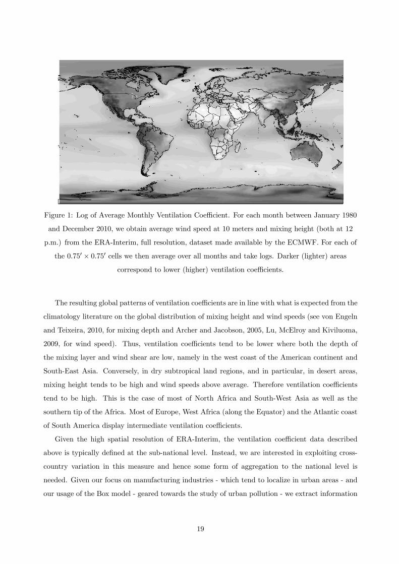
Figure 1: Log of Average Monthly Ventilation Coefficient. For each month between January 1980

and December 2010, we obtain average wind speed at 10 meters and mixing height (both at 12

p.m.) from the ERA-Interim, full resolution, dataset made available by the ECMWF. For each of

the 0750 × 0750 cells we then average over all months and take logs. Darker (lighter) areascorrespond to lower (higher) ventilation coefficients.

The resulting global patterns of ventilation coefficients are in line with what is expected from the

climatology literature on the global distribution of mixing height and wind speeds (see von Engeln

and Teixeira, 2010, for mixing depth and Archer and Jacobson, 2005, Lu, McElroy and Kiviluoma,

2009, for wind speed). Thus, ventilation coefficients tend to be lower where both the depth of

the mixing layer and wind shear are low, namely in the west coast of the American continent and

South-East Asia. Conversely, in dry subtropical land regions, and in particular, in desert areas,

mixing height tends to be high and wind speeds above average. Therefore ventilation coefficients

tend to be high. This is the case of most of North Africa and South-West Asia as well as the

southern tip of the Africa. Most of Europe, West Africa (along the Equator) and the Atlantic coast

of South America display intermediate ventilation coefficients.

Given the high spatial resolution of ERA-Interim, the ventilation coefficient data described

above is typically defined at the sub-national level. Instead, we are interested in exploiting cross-

country variation in this measure and hence some form of aggregation to the national level is

needed. Given our focus on manufacturing industries - which tend to localize in urban areas - and

our usage of the Box model - geared towards the study of urban pollution - we extract information

19

on the ventilation coefficient of each country’s capital city.38 To do this, we select the grid-cell that is

nearest to the capital city and assign to the latter the average ventilation coefficient of the former.39

We then take the ventilation coefficient of a country to be given by that of its capital. Figure 2

below presents the resulting country map. Given the high spatial correlation of our source measure

across grid-cells it is not surprising that the cross-country distribution of ventilation coefficients

obtained in this fashion largely mirrors the one discussed above.40

Figure 2: Log of Average Monthly Ventilation Coefficient in each country’s capital. For each

month between January 1980 and December 2010, we obtain average wind speed at 10 meters and

mixing height (both at 12 p.m.) from the ERA-Interim, full resolution, dataset made available by

the ECMWF. For each of the 0750 × 0750 cells we compute its distance to the nearest capitalcity. The ventilation coefficient in each capital is then given by the value of the nearest cell. As

before we average over all months and take logs. Darker (lighter) areas correspond to lower

(higher) ventilation coefficients in a country’s capital

Finally, and looking ahead to the next section, it is important to assess whether our ventila-

tion coefficient measure correlates with other traditional country-level determinants of comparative

advantage such as capital or skill abundance. We find that in our sample of countries there is

38As an alternative we have considered taking the ventilation coefficient corresponding to the largest city in each

country. The correlation between the largest city and the capital city measure is high and all of our results below are

robust to considering this alternative measure. We prefer to use the capital city ventilation coefficient as our baseline

measure since, for historical reasons, the location of a country’s capital is unlikely to reflect concerns on whether its

atmospheric conditions lead to more or less pollution dispersion.39We compute this distance based on the coordinates at the center of each grid-cell in the ERA-Interim dataset

and the coordinates of the capital city for each country.40For that reason, if we take as an alternative country measure the simple average over the ventilation coefficients

of all cells corresponding to each country we obtain a very similar distribution. The cross-country correlation between

this alternative measure and our baseline, capital city, measure is 0.88 and significant at the 1% level.

20

no significant correlation: the correlation with capital abundance, skill abundance and GDP per

capita is, respectively −003, −001 and −0005. Further, none of these correlations are statisticallysignificant at the 10% level. Further, our measure is only weakly correlated with oil reserves per

capita (014, p-value of 0.09) and fertile land per capita (−015, p-value of 0.07).

6 Instrumental Variables

6.1 Reduced Form Results

In this section we study the effects of clean air endowments on comparative advantage in polluting

industries. Thus, we analyze the direct effect of the ventilation coefficient on exports in polluting

industries. As argued above, as clean air is a public good, country-level endowments affect com-

parative advantage in polluting goods only through their influence in environmental regulation.

Thus, in the following section we use the ventilation coefficient as an instrument for environmental

regulation. In this section we perform a simpler exercise: we estimate reduced form effect of clean

air endowments on comparative advantage in polluting industries. This estimate is interesting in

its own right because it is independent from the particular measure of air pollution regulation used

and from the argument that clean air endowments only affects comparative advantage only through

regulation. We thus estimate the following specification:

= 1 × + 2 × + 3 × + 4 × + 5 × + + + , (13)

where is the ventilation coefficient in the capital of country , is GDP per capita,

is oil reserves per capita and is oil intensity for industry . Estimation results are reported in

Table 8. Column 1 estimates 1 without including any control, and the remaining columns add

controls sequentially. The first important result is that the effect of the ventilation coefficient on

comparative advantage in polluting industries (1) is always positive, stable across specifications

and significant at 1%. The main concern to interpret the estimates of 1 as the effect of the clean

air endowment on comparative advantage in polluting industries is that the ventilation coefficient

in the capital is determined by geographical and weather characteristics that could in principle

also influence a country´s level of development and thus its comparative advantage. In this case,

1 could be capturing the effect of a country´s level of development on exports of polluting goods

instead of the effect of the clean air endowment. The results reported in columns 1 and 2 indicate

that this is not the case: the estimated 1 is virtually unaffected by the inclusion of a control for

the interaction of GDP per capita and pollution intensity, suggesting that 1 is indeed capturing

21

the effect of the clean air endowment on comparative advantage. The inclusion of controls for

the oil, skill and capital interactions also have minor effects on the estimated 1 The estimated

coefficient on the on the ventilation and pollution interaction (×) reported in column 5 implies

that if a country moves from the mean to a one standard deviation below the mean in air pollution

regulation, the predicted relative import share of an industry that is one standard deviation above

the mean pollution intensity increases by 4.5% of a standard deviation.

6.2 Instrumental Variable Strategy

Can we interpret the OLS results presented in Section 4 as the causal effect of environmental

regulation on comparative advantage? As discussed above, an alternative interpretation is that

comparative advantage in polluting industries influences environmental regulation. This reverse

causality channel could upwards bias the estimated effect of environmental regulation if a country

with a comparative advantage in polluting industries faces a stronger industry lobby to enact

lax environmental regulations. On the contrary, our estimates could be downwards biased if a

comparative advantage in polluting industries results in higher levels of pollution, which induce

the population to demand clean air regulations. To address this concern we need an instrument

for environmental regulation. That is, a source of variation in environmental regulation that is

not determined by comparative advantage in polluting industries (exogenous) and does not affect

comparative advantage through other channels (exclusion restriction). As discussed above, the

ventilation coefficient is exogenous because it is determined by invariant weather and geographical

characteristics. It also arguably satisfies the exclusion restriction. The main concern on this respect

is that these geographical and weather characteristics could also influence a country´s level of

development or endowments of other production factors and thus shape its comparative advantage

through these other channels. The simple correlations in the data reported above suggest that this

is not the case: the correlation coefficient of the ventilation coefficient and GDP per capita, capital

and skill endowments are between -0.005 and 0.03 and not statistically different from zero. The

almost zero correlation between the ventilation coefficient and other determinants of comparative

advantage suggest that the exclusion restriction is satisfied. Still, we include them as controls in

what follows.

Our instrumental variable estimation strategy follows the following steps. In the first stage we

estimate the following equation:

× = 1 × + 2 × + 3 × + 4 × + + + , (14)

22

where the dependent variable is the interaction of environmental regulation in country and

pollution intensity in industry ( × ) and our excluded instrument is the interaction of the

ventilation coefficient in country and pollution intensity in industry ( × ). In the second

stage we estimate the following equation:

= 1 \ × + 2 × + 3 × + 4 × + + + (15)

where \ × = b1 × + b2 × + b3 × + b4 × + b + b and bb are coefficientestimates of equation 14.

6.2.1 First Stage Results

Note that the only term of the pollution interaction that we instrument is environmental regulation

(), not pollution intensity () as it is measured using lagged U.S. industry characteristics thus

it is arguably exogenous to a particular country´s exports. Thus, before turning to the discussion

of the first stage results, we report the effect of the ventilation box coefficient on country-level

environmental regulation. Table 9 reports coefficient estimates of a regression of lax environmental

regulation () on the ventilation coefficient (). The estimated coefficient reported in column

1 indicates that a one standard deviation increase in the ventilation coefficient induces a 22% of

a standard deviation decrease in the stringency of environmental regulation. Subsequent columns

show that this estimate is robust to the inclusion of other country characteristics like per capita

GDP, fertile land per capita, oil reserves per capita, capital and skill endowments and the efficiency

of legal institutions. Note in particular that the inclusion for a control for GDP per capita in

column 2 does not significantly affect the estimated effect of the ventilation coefficient on envi-

ronmental regulation. This evidence supports the exclusion restriction: the ventilation coefficient

has a direct effect on environmental regulation and is not capturing the effect of geographical or

weather characteristics on the level of income. This is crucial because income per capita can affect

the demand for environmental regulation and shape comparative advantage. Similarly, the sta-

bility of the coefficient when controls for other country characteristics are included suggests that

the exclusion restriction is satisfied. The relationship between environmental regulation () on

the ventilation coefficient () is illustrated in Figure 3, where country names are included. Fitted

values correspond to the regression reported in column 2, where GDP per capita is included as a

control.

Next, we turn to the estimation of the first stage regression described in equation 14, reported in

Table 10. The first column includes only the interaction of the ventilation coefficient and pollution

23

intensity (×) and the rest of the columns add the remaining controls sequentially. The estimatedcoefficient on × is positive, stable and statistically significant at 1% in all specifications. The

F-test on the excluded instrument ( × ) varies between a value of 152 in column 1 where no

controls are included and 125.56 in the last column where all controls are included.

6.2.2 Second Stage Results

Panel A in Table 11 reports estimation of the second stage regression described in equation 15.

The first column includes only the (instrumented) interaction between environmental regulation

and pollution intensity ( \ × ) and the rest of the columns add the remaining controls sequen-

tially. The estimated coefficient on \ × (1) is positive, stable and statistically significant at

1% in all specifications. The stability of the estimated coefficient when controls for other country

characteristics are included suggests that the exclusion restriction is satisfied: the ventilation coeffi-

cient affects comparative advantage through its effect on environmental regulation, not because it is

correlated with other sources of comparative advantage. The estimated coefficient on the pollution

interaction ( × ) reported in column 3, where controls for the capital and skill interactions are

included, implies that if a country moves from the mean to a one standard deviation below the

mean in air pollution regulation, the predicted relative import share of an industry that is one

standard deviation above the mean pollution intensity increases by 18,6% of a standard deviation.

Panel B in Table 11 reports OLS estimation of an equation equivalent to 15. The OLS baseline

estimate of 1 is 10,8%, as reported in column 3. Then, our baseline instrumental variable estimates

of the effect of environmental regulation on comparative advantage in polluting industries are

around 80% higher than OLS estimates. This finding has two possible interpretations. First, OLS

estimates could be biased if comparative advantage in polluting industries influences environmental

regulation. Second, our measure of environmental regulation is at best partial, thus OLS estimates

might be downward biased due to measurement error. The first interpretation is related to our

discussion of reverse causality at the beginning if this section. Reverse causality could upwards

bias the estimated effect of environmental regulation if a country with a comparative advantage

in polluting industries faces a stronger industry lobby to enact lax environmental regulations. On

the contrary, our estimates could be downwards biased if a comparative advantage in polluting

industries results in higher levels of pollution, which induce the population to demand clean air

regulations. Our instrumental variables results suggest that this second channel could be operative.

In particular, some advanced countries that industrialized earlier might have faced stronger demand

from their citizens to address air pollution problems. Thus, if these countries tend to export more

in polluting industries but also have more stringent environmental regulation OLS estimates of

24

1 can be downwards biased. The second interpretation is highly plausible, as our measure of

environmental regulation only captures one dimension of air pollution regulation that is easily

comparable across countries, thus it is subject to measurement error. Thus, the results suggest

that our instrument captures the variation in the environmental regulation measure that is directly

driven by the broader effect of meteorological conditions on the demand for cleaner air and air

pollution policy.

7 Final Remarks

TO BE WRITTEN

References

[1] Abt Associates Inc., (2009). “Trade and Environmental Assessment Model: Model Descrip-

tion,” prepared for the U.S. Environmental Protection Agency National Center for Environ-

mental Economics/Climate Economics Branch, Cambridge MA: Abt Associates.

[2] Antras, P., (2003). “Firms, Contracts, and Trade Structure,” Quarterly Journal of Economics

118, 1375-418.

[3] Antweiler, W., B. Copeland, and S. Taylor, (2001). “Is Free Trade Good for the Environment?”

American Economic Review 91, 877-908.

[4] Archer, C., and M. Jacobson, (2005). “Evaluation of Global Wind Power,” Journal of Geo-

physical Research - Atmospheres 110, D12110.

[5] Associated Octel, (1996). “Worldwide Gasoline and Diesel Fuel Survey,” London: Associated

Octel Ltd.

[6] Beck, T., (2003). “Financial Dependence and International Trade,” Review of International

Economics 11, 296-316.

[7] Becker, R., and J. Henderson, (2000). “Effects of Air Quality Regulations on Polluting Indus-

tries,” Journal of Political Economy 108, 379-421.

[8] Besley, T., and T. Persson, (forthcoming). “The Origins of State Capacity: Property Rights,

Taxation and Politics,” American Economic Review.

25

[9] Brunnermeier, S., and A. Levinson, (2004). “Examining the Evidence on Environmental Reg-

ulations and Industry Location,” Journal of the Environment and Development 13, 6-41.

[10] Chichilnisky, G., (1994). “North-South Trade and the Global Environment,” American Eco-

nomic Review 84, 851-74.

[11] Chor, D., (2010). “Unpacking Sources of Comparative Advantage: A Quantitative Approach,”

Journal of International Economics 82, 152-67.

[12] Cole, M., R. Elliott, and P. Fredriksson, (2006). “Endogenous Pollution Havens: Does FDI

Influence Environmental Regulations?” Scandinavian Journal of Economics 108, 157-78.

[13] Cole M., R. Elliott, and K. Shimamoto, (2005). “Industrial Characteristics, Environmental

Regulations and Air Pollution: An Analysis of the U.K. Manufacturing Sector,” Journal of

Environmental Economics and Management 50, 121-43.

[14] Copeland, B., (1994). “International Trade and the Environment: Policy Reform in a Polluted

Small Open Economy,” Journal of Environmental Economics and Management 26, 44-65.

[15] Copeland, B., and M. Taylor, (1994). “North-South Trade and the Environment,” Quarterly

Journal of Economics 109, 755-87.

[16] Copeland, B., and M. Taylor, (1995). “Trade and Transboundary Pollution,” American Eco-

nomic Review 85, 716-37.

[17] Copeland, B., and M. Taylor, (2003). Trade and the Environment: Theory and Evidence,

Princeton University Press.

[18] Copeland, B., and M. Taylor, (2004). “Trade, Growth, and the Environment,” Journal of

Economic Literature 42, 7-71.

[19] Costinot, A., (2009). “On the Origins of Comparative Advantage,” Journal of International

Economics 77, 255-64.

[20] Cuñat, A., and M. Melitz, (forthcoming). “Volatility, Labor Market Flexibility, and the Pattern

of Comparative Advantage,” Journal of the European Economic Association.

[21] Damania, R., P. Fredriksson, and J. List, (2003). “Trade Liberalization, Corruption, and

Environmental Policy Formation: Theory and Evidence,” Journal of Environmental Economics

and Management 46, 490-512.

26

[22] Dasgupta, S., A. Mody, D. Roy, and D. Wheeler, (2001). “Environmental Regulation and

Development: A Cross-country Empirical Analysis,” Oxford Development Studies, Taylor and

Francis Journals, 29, 173-87.

[23] De Leeuw, F., E. van Zantvoort, R. Sluyter, and W. van Pul, (2002). “Urban Air Quality

Assessment Model: UAQAM,” Environmental Modeling & Assessment 7, 243-58.

[24] Dee, D.P. et al (2011), The ERA-Interim Reanalysis: Configuration and Performance of the

Data Assimilation System, Quarterly Journal of the Royal Meteorological Society, 137, pp.

553-597, April.

[25] Eaton, J., and S. Kortum, (2002). “Technology, Geography, and Trade,” Econometrica 70,

1741-79.

[26] Ederington, J., A. Levinson, and J. Minier, (2005). “Footloose and Pollution-free,” Review of

Economics and Statistics 87, 92-9.

[27] Ederington, J., and J. Minier, (2003). “Is Environmental Policy a Secondary Trade Barrier?

An Empirical Analysis,” Canadian Journal of Economics 36, 137-54.

[28] Environmental Protection Agency (2005), Basic Air Pollution Meteorology, E.P.A., Air Pollu-

tion Training Institute. Research Triangle Park, NC.

[29] Environmental Protection Agency (2004), Risk Assessment and Modeling - Air Toxics Risk

Assessment, Volume 1 - Technical Resource Manual. E.P.A., Office of Air Quality Planning

and Standards, Emissions Standards Division, Research Triangle Park, NC.

[30] Esty, D., M. Levy, T. Srebotnjak, and A. Sherbinin, (2005). 2005 Environmental Sustainabil-

ity Index: Benchmarking National Environmental Stewardship. New Haven: Yale Center for

Environmental Law & Policy.

[31] Feenstra, R., J. Romalis, and P. Schott, (2002). “U.S. Imports, Exports and Tariff Data,

1989-2001,” NBER Working Paper 9387.

[32] Greenstone, M., (2002). “The Impacts of Environmental Regulations on Industrial Activity:

Evidence from the 1970 and 1977 Clean Air Acts and the Census of Manufactures,” Journal

of Political Economy 110, 1175-219.

[33] Grossman, G., and A. Krueger, (1993). “Environmental Impacts of a North American Free

Trade Agreement,” in The U.S.-Mexico Free Trade Agreement, P. Garber ed., MIT Press,

13-56.

27

[34] Grossman, G., and A. Krueger, (1995). “Economic Growth and the Environment,” Quarterly

Journal of Economics 110, 353-77.

[35] Hall, R., and C. Jones, (1999). “Why Do Some Countries Produce So Much More Output per

Worker than Others?” Quarterly Journal of Economics, 14, 83-116.

[36] Hettige, H., P. Martin, M. Singh, and D. Wheeler (1995). “The Industrial Pollution Projection

System,” World Bank Policy Research Working Paper 1431.

[37] Hilton, F. G. H. and Levinson, A. M., 1998. Factoring the environmental Kuznets curve: evi-

dence from automotive lead emissions, Journal of Environmental Economics and Management,

35: 126-41.

[38] Jacobson, Marc Z. (2002), Atmospheric Pollution. History, Science and Regulation, Cambridge

University Press

[39] Middleton, D.R. (1998), A New Box Model to Forecast Urban Air Quality: BOXURB, Envi-

ronmental Monitoring and Assessment, Vol 52, 1-2, pp 315-335.

[40] Munn, R.E. (1976), Air Pollution Metereology, in Urban Air Quality Management, M.J. Suess

and S.R. Craxford (eds.), WHO Regional Publications, European Series N. 1, World Health

Organization, Copenhagen.

[41] Jaffe, A., S. Peterson, P. Portney, and R. Stavins, (1995). “Environmental Regulations and

the Competitiveness of U.S. Manufacturing: What Does the Evidence Tell Us?” Journal of

Economic Literature 33, 132-63.

[42] Keller, W., and A. Levinson, (2002). “Pollution Abatement Costs and Foreign Direct Invest-

ment Inflows to U.S. States,” Review of Economics and Statistics 84, 691-703.

[43] Kudamatsu, M., T. Persson and D. Stromber (2011), Weather and Infant Mortality in Africa",

mimeo IIES, Stockholm University.

[44] Leontief, W., (1970) “Environmental Repercussions and the Economic Structure: An Input-

Output Approach.” Review of Economics and Statistics, 52(3): 262—71.

[45] Levchenko, A., (2007). “Institutional Quality and International Trade,” Review of Economic

Studies 74, 791-819.

[46] Levinson, A., (2009). “Technology, International Trade, and Pollution from U.S. Manufactur-

ing,” American Economic Review 99, 2177-92.

28

[47] Levinson, A., and S. Taylor, (2008). “Unmasking the Pollution Haven Effect,” International

Economic Review 49, 223-54.

[48] List, J., D. Millimet, P. Fredriksson, and W. McHone, (2003). “Effects of Environmental

Regulations on Manufacturing Plant Births: Evidence From a Propensity Score Matching

Estimator,” Review of Economics and Statistics 85, 944-52.

[49] List, J., and D. Sturm, (2006). “How Elections Matter: Theory and Evidence from Environ-

mental Policy,” Quarterly Journal of Economics 121, 1249-81.

[50] Lovei, M., (1998). “Phasing Out Lead From Gasoline, Worlwide Experience and Policy Impli-

cations,” World Bank Technical Paper 397, Pollution Management Series.

[51] Lu, X. M.B. McElroy and J. Kiviluoma (2009), Global Potential for Wind-Generated Electric-

ity, Proceedings of the National Academies of Sciences, vol 106, n. 27, pp. 10933-10938.

[52] Lu, Z., D. G. Streets, Q. Zhang, S. Wang, G. R. Carmichael, Y. F. Cheng, C. Wei, M. Chin,

T. Diehl, and Q. Tan, (2010). “Sulfur Dioxide Emissions in China and Sulfur Trends in East

Asia,” Atmospheric Chemistry and Physics 10, 6311-31.

[53] Mani, M., and D. Wheeler, (1999). “In Search of Pollution Havens? Dirty Industry Migration

in the World Economy,” in Trade, Global Policy and the Environment, P. Frederiksson ed.,

World Bank Discussion Paper 402.

[54] Manova, K., (2008). “Credit Constraints, Heterogeneous Firms, and International Trade,”

NBER Working Paper 14531.

[55] McGuire, M., (1982). “Regulation, Factor Rewards, and International Trade,” Journal of Pub-

lic Economics 17: 335-54.

[56] Nunn, N., (2007). “Relationship-Specificity, Incomplete Contracts and the Pattern of Trade,”

Quarterly Journal of Economics 122, 569-600.

[57] Pethig, R., (1976). “Pollution, Welfare, and Environmental Policy in the Theory of Compara-

tive Advantage,” Journal of Environmental Economics and Management 2, 160-9.

[58] Rauscher, M., (1997). International Trade, Factor Movements, and the Environment. Oxford

University Press.

[59] Romalis, J., (2004). “Factor Proportions and the Structure of Commodity Trade,” American

Economic Review 94, 67-97.

29

[60] Vittal Murty, K. P. R., D. V. Viswanadham, Y. Sadhuram. (1980) Mixing heights and venti-

lation coefficients for urban centres in India. Boundary-Layer Meteorology 19:4, 441-451.

[61] Von Engeln, A. and J. Teixeira (2010), A Planetary Boundary Layer Height Climatology

derived from ECMWF Re-analysis Data, mimeo. Satellite Atmospheric Science Group, Lulea

University of Technology.

[62] World Bank, (2004). Doing Business in 2004: Understanding Regulation, World Bank and

Oxford University Press.

[63] World Economic Forum, (2004). The Global Competitiveness Report 2003-2004, M. Porter, K.

Schwab, X. Sala-i-Martin, and A. Lopez-Claro eds., Oxford University Press.

8 Appendix 1 Proof of Result 2

Taking the derivative of Equation (8) with respect to and rearranging we obtain

∗

= ·−1 ·

³∗´· 00

³

³∗´´+ · 0

³

³∗´´

2 · 00³ · ∗

´− 2 ·2· · 00

³

³∗´´ .

The denominator is positive because 00 0 and 00 0. If = 0, the numerator is negative

because 00 0 and the second term disappears. This proves the first result. Otherwise, since

1 and 0 0, the numerator is smaller than

¡∗¢ · 00 ¡ ¡∗ ¢¢+ 0

¡¡∗¢¢,

which is negative if − · 00 ()/ 0 () 1. This proves the second result.

9 Appendix 2: The Box model

The model determines the concentration of pollutants within the box {( ) : ∈ [0 ] , ∈ [0 ] , ∈ [0 ]}.The concentration of pollutants does not depend on height since vertical dispersion is instanta-

neous. Thus, let ( ) denote pollution at ( ) at time for all ∈ [0 ]. Wind blows inthe ascending direction.

30

Consider the sub-box {(0 0 0) : 0 ∈ [0 ] , 0 ∈ [0 ] , 0 ∈ [0 ]}. The change in total pollu-tion within the sub-box is given by

Z

0

Z

0

¡0 0

¢ · · 0 · 0 = · ·−Z

0

¡0

¢ · · · 0, (16)

where is mixing height, is wind speed, and is emissions per unit area. The first term on the

right hand side is the pollution emmitted within the sub-box and the second term is the pollution

that leaves the sub-box. The latter depends on the concentration of pollution at the downwind side

and the speed at which dirty air leaves the sub-box.

In steady state, the total pollution within the sub-box is constant and, thus, we have

Z

0

¡0

¢ · 0 = · ·

· , (17)

where we have ommited the time dependence. Taking the derivative of Equation (17) with respect

to we find

( ) = ·

· . (18)

Note that the concentration of pollutants is not constant within the urban area. It is zero at the

upwind edge of the urban area and increases linearly with distance from this edge.

The average concentration of pollution in the urban area is

=1

2·Z

0

Z

0

( ) · · . (19)

Given Equation (18), this implies

=

2·

· . (20)

31

Table 1: Ten most pollution intensive manufacturing industries for each pollutant.

Emission Factors are in Tons per million of dollars shipped.

NOx S02 CO

Rank Industry EF %Total Industry EF %Total Industry EF %Total

1 Lime and gypsum 6.68 1 Pulp/paper/paperboard mills 5.17 14 Alumina and aluminum 14.2 7

2 Cement and concrete 5.42 10 Lime and gypsum 4.85 1 Iron/Steel Mills and Ferroalloy 7.94 7

3 Glass and glass products 3.8 3 Nonferrous Metal(not Aluminum) 4.67 4 Lime and Gypsum 7.08 1

4 Pulp/paper/paperboard mills 3.67 10 Cement and concrete 4.22 7 Pulp/paper/paperboard mills 5.56 7

5 Pesticide & fertilizer 2.22 2 Alumina and Aluminum 4.19 4 Other Nonmetallic Mineral 4.81 1

6 Basic Chemicals 1.96 8 Pesticide & fertilizer 3.18 2 Steel Products 4.62 1

7 Petroleum and Coal Products 1.42 12 Basic Chemicals 2.69 11 Cement and Concrete 4.44 3

8 Veneer/Plywood/Eng. Wood 1.19 1 Petroleum and Coal Products 2.30 18 Basic Chemicals 4.36 8

9 Iron/Steel Mills and Ferroalloy 1.14 2 Other Chemical Products 1.89 3 Veneer/Plywood/Eng.Wood 3.29 1

10 Clay Product and Refractory 1.08 1 Veneer/Plywood/Eng. Wood 1.72 3 Nonferrous Metal(not Alum.) 3.24 1

% of Total Accounted by top 10 50 % of Total Accounted by top 10 66 % of Total Accounted by top 10 38

Emission Factors are in Tons per million of dollars shipped. "% Total" gives the industry’s share of total

emissions in manufacturing.

Table 2: Rank correlation of pollution intensity ranking of industries.

NOx SO2 CO

NOx 1 - -

SO2 0.58∗∗∗ 1 -

CO 0.90∗∗∗ 0.44∗∗∗ 1∗∗∗ indicates significance at the 1 percent level.

Table 3: Correlation between Pollution, Skill and Capital Intensities.

NOx SO2 CO

1 - -

Skill Intensity -0.24∗∗ -0.19∗ -0.25∗∗

Capital Intensity 0.33∗∗∗ 0.52∗∗∗ 0.53∗∗∗∗ indicates significance at the 10 percent level,∗∗ indicates significance at the 5 percent level, ∗∗∗ at 1

per cent level.

33

Table 4: Grams of Lead per Liter of Gasoline: the ten least and ten most stringent

countries

Rank Most Stringent Regulation Value Least Stringent Regulation Value

1 Sweden 0 Venezuela 0.85

2 Denmark 0 Burkina Faso 0.84

3 Finland 0 Burundi 0.84

4 Japan 0 Cameroon 0.84

5 Canada 0 Chad 0.84

6 Austria 0 Cuba 0.84

7 Bolivia 0 Lebanon 0.84

8 Guatemala 0 Uganda 0.84

9 Brazil 0 Zimbabwe 0.84

10 Thailand 0 Benin 0.84

Median is 0.38, mean is 0.36. South Africa is the country closes to the global mean.

Source: Lovei (1998)

34

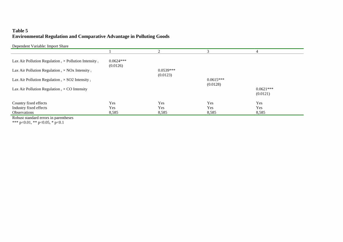
Table 5 Environmental Regulation and Comparative Advantage in Polluting Goods Dependent Variable: Import Share 1 2 3 4 Lax Air Pollution Regulation c × Pollution Intensity i 0.0624*** (0.0126) Lax Air Pollution Regulation c × NOx Intensity i 0.0539*** (0.0123) Lax Air Pollution Regulation c × SO2 Intensity i 0.0615*** (0.0128) Lax Air Pollution Regulation c × CO Intensity 0.0621*** (0.0121) Country fixed effects Yes Yes Yes Yes Industry fixed effects Yes Yes Yes Yes Observations 8,585 8,585 8,585 8,585 Robust standard errors in parentheses *** p<0.01, ** p<0.05, * p<0.1

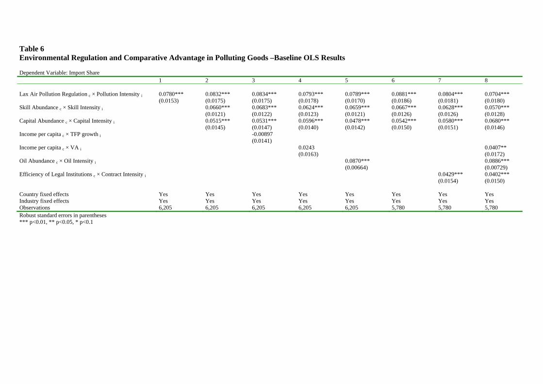
Table 6 Environmental Regulation and Comparative Advantage in Polluting Goods –Baseline OLS Results Dependent Variable: Import Share 1 2 3 4 5 6 7 8 Lax Air Pollution Regulation c × Pollution Intensity i 0.0780*** 0.0832*** 0.0834*** 0.0793*** 0.0789*** 0.0881*** 0.0804*** 0.0704*** (0.0153) (0.0175) (0.0175) (0.0178) (0.0170) (0.0186) (0.0181) (0.0180) Skill Abundance c × Skill Intensity i 0.0660*** 0.0683*** 0.0624*** 0.0659*** 0.0667*** 0.0628*** 0.0570*** (0.0121) (0.0122) (0.0123) (0.0121) (0.0126) (0.0126) (0.0128) Capital Abundance c × Capital Intensity i 0.0515*** 0.0531*** 0.0596*** 0.0478*** 0.0542*** 0.0580*** 0.0680*** (0.0145) (0.0147) (0.0140) (0.0142) (0.0150) (0.0151) (0.0146) Income per capita c × TFP growth i -0.00897 (0.0141) Income per capita c × VA i 0.0243 0.0407** (0.0163) (0.0172) Oil Abundance c × Oil Intensity i 0.0870*** 0.0886*** (0.00664) (0.00729) Efficiency of Legal Institutions c × Contract Intensity i 0.0429*** 0.0402*** (0.0154) (0.0150) Country fixed effects Yes Yes Yes Yes Yes Yes Yes Yes Industry fixed effects Yes Yes Yes Yes Yes Yes Yes Yes Observations 6,205 6,205 6,205 6,205 6,205 5,780 5,780 5,780 Robust standard errors in parentheses *** p<0.01, ** p<0.05, * p<0.1

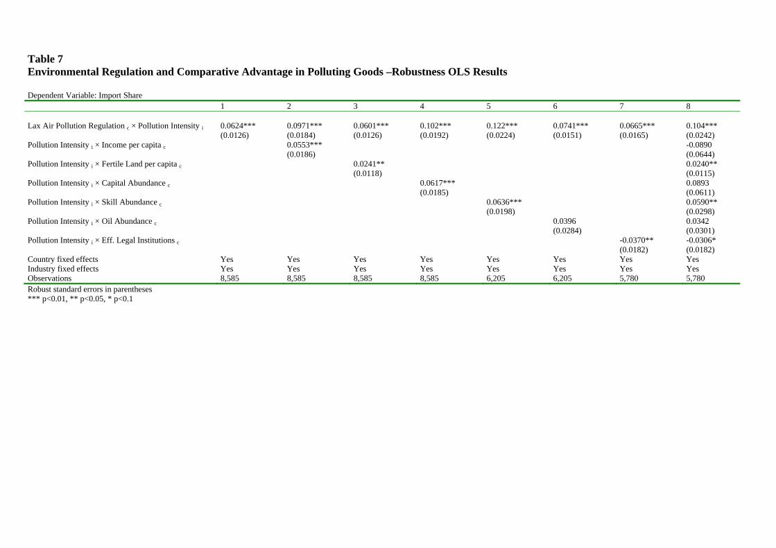
Table 7 Environmental Regulation and Comparative Advantage in Polluting Goods –Robustness OLS Results Dependent Variable: Import Share 1 2 3 4 5 6 7 8 Lax Air Pollution Regulation c × Pollution Intensity i 0.0624*** 0.0971*** 0.0601*** 0.102*** 0.122*** 0.0741*** 0.0665*** 0.104*** (0.0126) (0.0184) (0.0126) (0.0192) (0.0224) (0.0151) (0.0165) (0.0242) Pollution Intensity i × Income per capita c 0.0553*** -0.0890 (0.0186) (0.0644) Pollution Intensity i × Fertile Land per capita c 0.0241** 0.0240** (0.0118) (0.0115) Pollution Intensity i × Capital Abundance c 0.0617*** 0.0893 (0.0185) (0.0611) Pollution Intensity i × Skill Abundance c 0.0636*** 0.0590** (0.0198) (0.0298) Pollution Intensity i × Oil Abundance c 0.0396 0.0342 (0.0284) (0.0301) Pollution Intensity i × Eff. Legal Institutions c -0.0370** -0.0306* (0.0182) (0.0182) Country fixed effects Yes Yes Yes Yes Yes Yes Yes Yes Industry fixed effects Yes Yes Yes Yes Yes Yes Yes Yes Observations 8,585 8,585 8,585 8,585 6,205 6,205 5,780 5,780 Robust standard errors in parentheses *** p<0.01, ** p<0.05, * p<0.1

Table 8 Ventilation Potential and Comparative Advantage in Polluting Goods –Reduced Form Results Dependent Variable: Import Share 1 2 3 4 5 6 7 Ventilation Potential c × Pollution Intensity i 0.0569*** 0.0570*** 0.0545*** 0.0454*** 0.0450*** 0.0455*** 0.0408*** (0.00978) (0.00977) (0.00949) (0.0119) (0.0119) (0.0119) (0.0113) Pollution Intensity i × Income per capita c 0.0167* 0.0128 -0.0148 -0.0184 (0.00995) (0.00970) (0.0139) (0.0136) Oil Abundance c × Oil Intensity i 0.0566*** 0.0792*** (0.0204) (0.00698) Skill Abundance c × Skill Intensity i 0.0578*** 0.0556*** 0.0545*** (0.0108) (0.0112) (0.0111) Capital Abundance c × Capital Intensity i 0.0231** 0.0314*** 0.0314*** (0.0113) (0.0121) (0.0121) Country fixed effects Yes Yes Yes Yes Yes Yes Yes Industry fixed effects Yes Yes Yes Yes Yes Yes Yes Observations 12,750 12,750 12,580 8,075 8,075 8,075 8,075 Robust standard errors in parentheses *** p<0.01, ** p<0.05, * p<0.1

Table 9 Ventilation Potential and Environmental Regulation Dependent Variable: Lax Environmental Regulation

1 2 3 4 5 6 7 8 9

Ventilation Potential c 0.219*** 0.211*** 0.220*** 0.218*** 0.184*** 0.218** 0.188** 0.217*** 0.230*** [0.0815] [0.0690] [0.0686] [0.0693] [0.0691] [0.0841] [0.0918] [0.0743] [0.0739]

Income per capita c -0.624*** -0.617*** -0.628*** -0.680*** -0.680*** -0.202 -0.659*** -0.564*** [0.0584] [0.0589] [0.0582] [0.0536] [0.0681] [0.305] [0.0610] [0.0723]

Fertile Land per capita c 0.0627 [0.0808]

Oil Abundance c 0.216*** [0.0584]

Skill Abundance c -0.351** [0.153]

Capital Abundance c -0.183 [0.281]

Efficiency Legal Institutions c -0.246*** [0.0848]

Observations 101 101 101 99 99 73 73 89 89 Robust standard errors in brackets *** p<0.01, ** p<0.05, * p<0.1

Table 10 Ventilation Potential and Environmental Regulation- First Stage Results Dependent Variable: Environmental Regulation c × Pollution Intensity i 1 2 3 4 5 6 7 8 9 10 11 Ventilation Potential c × Pollution Intensity i 0.219*** 0.211*** 0.218*** 0.217*** 0.191*** 0.186*** 0.186*** 0.201*** 0.206*** 0.203*** 0.213*** [0.0177] [0.0149] [0.0181] [0.0181] [0.0198] [0.0218] [0.0227] [0.0190] [0.0189] [0.0189] [0.0190] Pollution Intensity i × Income per capita c -0.624*** -0.680*** -0.656*** -0.671*** -0.632*** -0.635*** -0.632*** [0.0126] [0.0147] [0.0174] [0.0159] [0.0195] [0.0194] [0.0194] Skill Abundance c × Skill Intensity i 0.0353*** 0.135*** 0.0232*** 0.0228*** 0.0248*** [0.00676] [0.0112] [0.00735] [0.00734] [0.00723] Capital Abundance c × Capital Intensity i -0.0217** -0.387*** -0.0146 -0.0145 -0.0129 [0.0109] [0.0161] [0.0116] [0.0116] [0.0117] Eff. of Legal Institutions c × Contract Intensity i 0.0880*** 0.0850*** 0.0836*** [0.0152] [0.0151] [0.0151] Oil Abundance c × Oil Intensity i 0.0423*** 0.0424*** [0.00705] [0.00667] Pollution Intensity i × Fertile Land per capita c 0.0627*** [0.0223] Country fixed effects Yes Yes Yes Yes Yes Yes Yes Yes Yes Yes Yes Industry fixed effects Yes Yes Yes Yes Yes Yes Yes Yes Yes Yes Yes Observations 8,585 8,585 6,205 6,205 6,205 6,205 5,780 5,780 5,780 5,780 5,780 Robust standard errors in brackets *** p<0.01, ** p<0.05, * p<0.1

Table 11 Environmental Regulation and Comparative Advantage in Polluting Goods. Panel A: Instrumental Variables Results Dependent Variable: Import Share 1 2 3 4 5 6 7 8 9 10 11 Lax Air Pollution Regulation c × Pollution Intensity i 0.237*** 0.246*** 0.193*** 0.186*** 0.207*** 0.219*** 0.246*** 0.231*** 0.238*** 0.213*** 0.232*** [0.0570] [0.0584] [0.0624] [0.0628] [0.0715] [0.0739] [0.0792] [0.0720] [0.0715] [0.0687] [0.0663] Pollution Intensity i × Income per capita c 0.149*** 0.105** 0.100** 0.123** 0.129*** 0.108** 0.122*** [0.0386] [0.0437] [0.0430] [0.0499] [0.0482] [0.0451] [0.0433] Skill Abundance c × Skill Intensity i 0.0668*** 0.0489*** 0.0625*** 0.0624*** 0.0628*** [0.0126] [0.0154] [0.0130] [0.0130] [0.0131] Capital Abundance c × Capital Intensity i 0.0350** 0.0988*** 0.0443*** 0.0442*** 0.0451*** [0.0142] [0.0304] [0.0149] [0.0148] [0.0148] Eff. of Legal Institutions c × Contract Intensity i 0.0349** 0.0315** 0.0292* [0.0153] [0.0149] [0.0149] Oil Abundance c × Oil Intensity i 0.0784*** 0.0776*** [0.00832] [0.00808] Pollution Intensity i × Fertile Land per capita c 0.0254** [0.0125] Country fixed effects Yes Yes Yes Yes Yes Yes Yes Yes Yes Yes Yes Industry fixed effects Yes Yes Yes Yes Yes Yes Yes Yes Yes Yes Yes Observations 8,585 8,585 6,205 6,205 6,205 6,205 5,780 5,780 5,780 5,780 5,780 Robust standard errors in brackets *** p<0.01, ** p<0.05, * p<0.1

Table 12 Environmental Regulation and Comparative Advantage in Polluting Goods. Panel B: OLS Results Dependent Variable: Import Share 1 2 3 4 5 6 7 8 9 10 11 Lax Air Pollution Regulation c × Pollution Intensity i 0.0624*** 0.0971*** 0.112*** 0.108*** 0.0832*** 0.0780*** 0.0815*** 0.110*** 0.101*** 0.0925*** 0.0910*** [0.0124] [0.0182] [0.0227] [0.0227] [0.0172] [0.0151] [0.0161] [0.0233] [0.0228] [0.0215] [0.0217] Pollution Intensity i × Income per capita c 0.0553*** 0.0501** 0.0497** 0.0425* 0.0438* 0.0325 0.0329 [0.0184] [0.0213] [0.0228] [0.0217] [0.0234] [0.0215] [0.0215] Skill Abundance c × Skill Intensity i 0.0701*** 0.0660*** 0.0664*** 0.0658*** 0.0669*** [0.0122] [0.0119] [0.0127] [0.0127] [0.0128] Capital Abundance c × Capital Intensity i 0.0331** 0.0515*** 0.0416*** 0.0418*** 0.0424*** [0.0140] [0.0143] [0.0147] [0.0147] [0.0147] Efficiency of Legal Institutions c × Contract Intensity i 0.0452*** 0.0400*** 0.0391*** [0.0153] [0.0147] [0.0147] Oil Abundance c × Oil Intensity i 0.0851*** 0.0856*** [0.00699] [0.00689] Pollution Intensity i × Fertile Land per capita c 0.0295*** [0.0112] Country fixed effects Yes Yes Yes Yes Yes Yes Yes Yes Yes Yes Yes Industry fixed effects Yes Yes Yes Yes Yes Yes Yes Yes Yes Yes Yes Observations 8,585 8,585 6,205 6,205 6,205 6,205 5,780 5,780 5,780 5,780 5,780 Robust standard errors in brackets *** p<0.01, ** p<0.05, * p<0.1