Source Identification and Apportionment of Atmospheric ...ijesd.org/papers/152-D579.pdf · Paul Chiou, Wei Tang, Jalpa Shah, Rafael Tadmor, and T.C. Ho International Journal of Environmental

Abstract—Ambient air samples of PM2.5 were collected at a

monitoring site in Port Arthur of Texas by US EPA (Environ- mental Protection Agency) from September of 2005 to June of 2009. A total of 343 samples with 53 species were measured and the data were analyzed by positive matrix factorization (PMF) to infer the sources of PM observed at the site. The analysis identified eleven source-related factors: sulfate-rich secondary aerosol (31.9%), motor vehicle (22.3%), aged sea-salt (11.1%), cement/carbon-rich (8.3%), airborne soil (7.4%), railroad traffic (5.7%), metal processing (3.1%), sea salt (3.0%), marine aerosol (2.8%), wood smoke (2.4%), and nitrate-rich secondary aerosol (1.9%). Basically, the factors of sulfate, airborne soil, and nitrate were likely to be regionally related sources. Motor vehicle, cement/carbon-rich, railroad traffic, metal processing, marine aerosol, and wood smoke factors were likely to be the local sources.

Index Terms—Airborne particulate matter, conditional probability function, positive matrix factorization, receptor modeling.

I. INTRODUCTION Port Arthur, Texas (29°53'06"N, 93°56'24"W) located on

the western bank of Sabine Lake, 130 km east of Houston and 25 km north of the Gulf of Mexico, is a medium size urban area in Southeast Texas. With two neighboring cities, Beaumont and Orange, it constitutes the so-called Golden Triangle in Texas, a major industrial area on the Texas Gulf Coast. Several major chemical plants, petrochemical plants, refineries, and waste management sites are located in Port Arthur. The Port Arthur monitoring site operated by US EPA is located at 2200 Jefferson Drive of Port Arthur. In an effort to better characterize the ambient air quality in Port Arthur of Texas, it is important to identify the possible sources of PM2.5 in the region. To understand the source/receptor relationship, multivariate receptor models have been applied to the observed speciated PM over the years. The multivariate approach is based on the fundamental principle that mass conservation can be assumed, and a mass balance analysis can be used to identify and apportion sources of airborne

Manuscript received June 20, 2011, revised September 30, 2011. This

work was supported in part by the US EPA through project R-07-0159. P. Chiou is with the Department of Mathematics, Lamar University, Box

10047, Beaumont, TX 77710, USA (e-mail: [email protected]). W. Tang was with Lamar University, Beaumont, TX 77710, USA. He is

now with the Department of Civil and Environmental Engineering, Rice University, Houston, TX 77005, USA (e-mail: [email protected]).

J. Shah was with the Department of Chemical Engineering, Lamar University, Beaumont, TX 77710, USA (e-mail: [email protected]).

R. Tadmor and T.C. Ho are with the Department of Chemical Engi- neering, Lamar University, Box 10053, Beaumont, TX 77710, USA (e-mail: [email protected] and [email protected]).

particulate matter in the atmosphere [1], [2]. Among the multivariate receptor models, positive matrix factorization (PMF) is a relatively new technique developed by [3]-[5]. It has been successfully applied to several source attribution studies [6]-[17].

The objectives of this study are to (i) identify the sources of particulate pollutants at the site, (ii) estimate the source contributions as well as source composition of each possible source [18]-[26], and (iii) investigate the regional-local source contrast using estimated source contributions and seasonal variations of each factor at the site. Such a study in this region of Texas has not been reported in earlier literature.

II. MATERIALS AND METHODS

A. Sampling and Measurements The PM2.5 composition sample data analyzed in this study

was downloaded from the US EPA website at http://www. epa.gov/ttn/airs/airsaqs/, and processed to conform to the PMF data format. The original 24-h integrated samples were collected at the Port Arthur monitoring site (29°55'22"N, 93°54'32"W) using a fine particle sequential sampler. The Port Arthur site, 4 km off the intersection between highway 69 and 73, is located 30 km southeast of Beaumont (Fig. 1). The sequential sampler used at the site was Partisol-Plus Model 2025 Sequential Air Sampler (Rupprecht/Patashnick Co. Inc.) with very sharp cut cyclone fractionators. Ambient air samples are drawn at a constant flow rate into a specially shaped inlet that removes particles with aerodynamic diameters greater than 2.5 μm, and the remaining particles are passed through a filter. Integrated 24-h PM2.5 particle samples were collected on Teflon filters. Total mass was then determined gravimetrically from the filters. Most of PM samples were collected every third day and some were collected every sixth day during the time period between September 2005 and June 2009. A total of 343 samples were obtained at the site. Both mass concentration and elemental chemical speciation were determined using an energy dis- persive X-ray fluorescence (XRF). An ion chromatography (IC) was used to analyze sulfate (SO 2

4− ), ammonium (NH 4

+ ), and nitrate (NO 3

− ) concentrations. The thermal optical trans- mission technique was used to measure both organic carbon (OC) and elemental carbon (EC). Each sample was characterized by 53 species, including: Ag, Al, As, Au, Ba, Br, Ca, Cd, Ce, Cl, Co, Cr, Cs, Cu, Eu, Fe, Ga, Hf, Hg, In, Ir, K, La, Mg, Mn, Mo, Na, Nb, Ni, P, Pb, Rb, S, Sb, Sc, Se, Si, Sm, Sn, Sr, Ta, Tb, Ti, V, Y, Zn, Zr, W, OC, EC, SO 2

4− , NH 4

+ , NO 3− .

In the data, the concentration of XRF S and SO 24

− were highly correlated (slope = 2.72, 2r = 0.94), thus it is reasonable to exclude XRF S from the analysis [10]. The

Source Identification and Apportionment of Atmospheric Aerosol over Port Arthur of Texas

Paul Chiou, Wei Tang, Jalpa Shah, Rafael Tadmor, and T.C. Ho

International Journal of Environmental Science and Development, Vol. 2, No. 5, October 2011

362

XRF analysis of PM2.5 speciation filters at sites in Texas was previously conducted by the Research Triangle Institute [19]. After October 31st, 2004, the XRF analysis of filters from all except three of Texas PM2.5 speciation sites was switched to the Desert Research Institute laboratory. It was found that about 90% of phosphorous concentrations at Texas sites were below detection limits prior to November 1st of 2004, while the phosphorous levels were suddenly above the detection limits after the laboratory change possibly due to analytical artifacts in the data [19]. The site used in this PMF analysis is among those switched to. Furthermore, there was a high correlation of 2r = 0.84 between phosphorous and sulfur at the Port Arthur site. On the other hand, 18 out of the 53 chemical species have a lower signal-to-noise ratio (S/N less than 0.4). As a result, these 18 species and phosphorous were also excluded in the PMF analysis. In the data matrix, there were missing values as well as below-detection-limit values. The comparison of measured PM mass to the sum of PM compositional data indicates that some of the measured PM mass concentrations were less than the sum of species concentrations. The analytical uncertainty estimates associated with each measured concentration and the detection limits for instruments were also reported. The possible source of measurement errors which can be considered as the uncertainty include the collection of over- and under- sized particles, the mass gain or loss of the collected PM mass, and the analytical sensitivity. Table I summarizes the PM2.5 speciation data used in this study.

Fig. 1. Location of Port Arthur monitoring site.

B. PMF and Data Handling In this study, PMF was used with the data collected at the

Port Arthur site as discussed previously. PMF is an approach of factor analysis, and it is described in detail by [3]. Only a brief description of this approach is provided here. PMF uses the method of weighted least-squares to solve a general receptor modeling problem. The general model assumes there are p sources, source types or source regions (termed factors) impacting a receptor and the observed concentrations of various species at the receptor are linear combinations of the impacts from the p factors. The factor analysis model (PMF) can be written as

1

1, ..., 1, ..., ,, ;p

ij ij ij ik kj ijk

n mx y e g f e i j=

= == + = +∑ (1)

where ijx is the jth species concentration measured in the ith sample, ikg is the particulate mass concentration from the kth source (or factor) contributing to the ith sample, kjf is the jth species mass fraction from the kth source (or factor),

ije is the residual associated with the jth species concentration measured in the ith sample, and p is the total number of sources (or factors).

The objective of PMF is to estimate the mass contributions ikg and the mass fractions (or profiles) kjf in (1) by the

weighted least-squares. The estimates of source contributions and source profiles are obtained by a unique algorithm in which both matrices G = [ ikg ] and F = [ kjf ] are adjusted in each iteration step. The process continues until convergence occurs [3], [14]. The application of PMF requires the estimated uncertainty ijs for each data value ijx to be carefully selected so that it reflects the quality and reliability of each data point. This important feature of PMF enables us to properly handle any below detection limit and missing data values. The uncertainty estimate provides a useful tool to decrease the weight of any below detection limit and missing data values when searching for the best estimates. In this study, the procedure of [14] was adopted as follows: (i) the concentration value ijx was the actually measured concentration, and the sum of the analytical uncertainty and one third of the detection limit value was used as the estimated uncertainty ijs if ijx was a determined value; (ii) the concentration value ijx was replaced by half of the detection limit value, and five sixths of the detection limit value was used as the estimated uncertainty ijs if ijx was below detection limit; (iii) the concentration value ijx was set equal to the geometric mean of all the measured values of ijx for element j, and its corresponding uncertainty ijs was set equal to four times of this geometric mean value if

ijx was a missing data value. Half of the average detection limits were used for below detection limits values in the calculation of the geometric means. Furthermore, the estimated uncertainties of OC and SO 2

4− were increased by a

factor of three because of its magnitude compared to the lower concentration species.

C. Robust Mode It is well-known that extreme data values as well as true

outliers can distort the least-squares estimation profoundly. A delicate handling of these data values is important, and PMF offers a robust mode to properly weigh these data points in the process of searching for the estimates. The robust factorization based on the Huber influence function [27] is a technique of iterative reweighing of the individual data values. The least squares approach with the robust factor analysis now leads to minimize Q

(2) where

and α is the outlier threshold distance. The value of 4.0α = was chosen in this study.

2

1 1

( / ) ,n m

ij ij iji j

Q e h s= =

=∑∑

2,

,

if

otherwise

1 | / || / | /

ij ijij

ij ij

e sh

e sα

α

≤=⎧⎨⎩


363

TABLE I: SUMMARY OF PM2.5 AND 33 SPECIES MASS CONCENTRATIONS USED FOR PMF ANALYSIS

Species Concentration (ngm-3) Number of BDLb values (%)

Number of missing values (%) Geometric meana Arithmetic mean Minimum Maximum

PM2.5 9503 10739 2542 53200 1 (0.3) 14 (4.1) Al 42.6 108.3 4.1 1946 33 (9.6) 4 (1.2) As 0.33 0.43 0 8.8 309 (90) 4 (1.2) Ba 1.6 4.2 0.4 128 301 (87.8) 4 (1.2) Br 2.2 3.1 0.6 30 163 (47.5) 4 (1.2) Ca 51.6 64.5 5.5 497 2 (0.6) 4 (1.2) Ce 1.5 3.7 0.6 35.7 334 (97.3) 4 (1.2) Cl 18.7 142.8 0.7 2547 37 (10.8) 4 (1.2) Co 0.2 0.3 0.1 1.4 335 (97.6) 4 (1.2) Cr 0.8 0.9 0.4 19.7 297 (86.6) 4 (1.2) Cu 1.3 1.8 0.6 34.7 230 (67.1) 4 (1.2) Fe 59.4 96.6 3.9 1262 3 (0.9) 4 (1.2) K 74.2 109.7 17.1 2028 3 (0.9) 4 (1.2) La 1.6 4.7 0.6 54.1 338 (98.5) 4 (1.2) Mg 28.3 46.9 7.8 545 214 (62.4) 4 (1.2) Mn 2.6 3.3 1 28.5 208 (60.6) 4 (1.2) Na 175 281.3 43.6 2327 114 (33.2) 4 (1.2) Ni 1.1 1.4 0.2 8.9 144 (42) 4 (1.2) Pb 2.5 2.9 0.8 17.7 281 (81.9) 4 (1.2) Sc 1.5 1.6 0.6 3.8 334 (97.3) 4 (1.2) Se 1.2 1.3 0 4.9 329 (95.9) 4 (1.2) Sm 2.2 5.7 0.8 42.4 336 (97.9) 4 (1.2) Si 70.6 195.6 2.9 3406 21 (6.1) 4 (1.2) Sr 1.8 2.3 0 36.9 225 (65.6) 4 (1.2) Tb 2.9 7.8 1.1 84.2 335 (97.6) 4 (1.2) Ti 4 8.6 0.6 128.8 78 (22.7) 4 (1.2) V 3.4 5 0.1 64.5 18 (5.2) 4 (1.2) Y 0.8 0.9 0.1 3.6 278 (81) 4 (1.2) Zn 7.8 11 0.4 188.5 13 (3.8) 4 (1.2) OC 2510 2939 1012 23364 9 (2.6) 3 (0.9) EC 286 352 31 1484 14 (4.1) 3 (0.9) SO 2

4− 2814 3326 484 12062 3 (0.9) 4 (1.2)

NH 4+ 918 1126 76 4596 3 (0.9) 4 (1.2)

NO 3− 149.4 256.1 1.1 1569 6 (1.7) 4 (1.2)

aData below the limit of detection were replaced by half of the reported detection limit values for the geometric mean calculations. bBelow detection limit.

D. Mass Apportionment Because of the mass closure violation noted previously,

the measured particle mass concentration was included as an independent variable in the PMF modeling to directly obtain the mass apportionment instead of using a regression analysis [9], [10]. The estimated uncertainties of the PM2.5 mass concentrations were set at four times of their values to reduce their weight in the model fit so that the magnitude of PM mass will not skew the analysis. When the measured particle mass concentration is included as an independent variable, the PMF apportions a mass concentration for each source

based on its temporal variation without using a multiple linear regression. The results of PMF modeling are then normalized by the apportioned particle mass concentrations so that the quantitative source contributions are obtained. Specifically,

1

( )( / ),p

ij k ik kj kk

x c g f c=

=∑ (3)

where kc denotes directly apportioned mass concentration by PMF for the kth factor.


364

E. Conditional Probability Function The conditional probability function (CPF) which calcu-

lates the probability that a source is located within a particular wind direction sector, θΔ , is defined by (4) where m θΔ is the number of occurrences that the source contribution exceeds the threshold criterion while the wind passes through sector θΔ , and n θΔ is the number of occurrences that the wind passes through direction sector

θΔ [9], [10], [28]. The source contribution estimates from PMF, coupled with wind direction values measured on site, were used to calculate the CPF. In order to minimize the effect of atmospheric dilution, however, daily fractional mass contribution from each source relative to the total contribution of all sources rather than the absolute source contribution was used [9], [10]. The same daily fractional mass contribution was assigned to each hour of a given day so that it was coupled with the hourly wind direction. The hourly time periods with wind speed less than 1 m/s were removed from the data set. The angular interval θΔ was set at 11.3 degrees, and the threshold criterion of upper 25% was used to show clear directionality of high conditional probability values.

III. RESULTS AND DISCUSSION An essential step in PMF analysis is to determine the

number of factors (sources) and source apportionment. For determination of the number of factors (sources), the basic consideration is to obtain a good fit of the model to the original data, and the model can well explain the physical meaning of the data. If there is goodness of fit, the theoretical value of Q in (2) should be approximately equal to the number of degrees of freedom or approximately equal to the number of entries in the data array provided that correct values of ijs have been used [29]. In a well-fit model, the residuals ije and the error estimates ijs should not be too much different in size, and the ratio ( / )ij ije s should fluctuate between ±3. Juntto and Paatero [8] recommended values of ±2 for the ratio. Based on the criterion of obtaining the most physically meaningful solution with the calculated Q value of 15,400 close to the theoretical Q value of 11,662, the PMF identified eleven source types by trial and error with different numbers of factors. We termed these factors as sulfate-rich secondary aerosol, motor vehicle, aged sea-salt, cement/carbon-rich, airborne soil, railroad traffic, metal processing, sea salt, marine aerosol, wood smoke, and nitrate-rich secondary aerosol.

Fig. 2 shows a relationship between the reconstructed PM2.5 mass contributions from all sources and the measured PM2.5 mass concentrations. It is clear that the resolved sources effectively reproduce the measured values and account for most of the variation in the PM2.5 mass concentrations (slope = 0.80 and 2r = 0.89). The average contributions (%) of these factors towards the PM mass, i.e.,

kc in (3) divided by the total mass from PMF analysis are summarized in Table II. Fig. 3 displays the identified source profile for each source at the site. Each source profile plot in Fig. 3 displays not only the profile estimate but also the lower

and upper limit of a 90% confidence interval for the mean profiles. These limits were obtained by a bootstrapping technique [30] combined with a method to account for the rotational freedom in the solution. The smaller magnitude the whisker, the more consistent the estimate is and the larger magnitude the whisker, the less consistent the result is. In other words, the smaller magnitude the whisker, the smaller associated error the estimate has and the larger magnitude the whisker, the larger associated error the estimate has. Fig. 4 presents the time series plots of estimated source contributions to PM2.5 mass concentrations for each source. The seasonal variations in the time series plots may be explained by variation in source strength, atmospheric transport, and possible chemical reactions in the atmosphere, or a combination of the three. The conditional probabilities of source direction (4) for each source are plotted in polar coordinates and displayed in Fig. 5. The average source contributions of each source to the PM2.5 concentrations in summer and winter are respectively presented in Fig. 6.

0 10 20 30 400

10

20

30

40

Pre

dict

ed p

artic

le m

ass

conc

. (μ g

/m3 )

Measured particle mass conc. (μg/m3)

R2=0.893

Fig. 2. Measured versus predicted PM mass concentration.

Among the eleven factors identified, the first factor is

sulfate-rich secondary aerosol. Fig. 3 and Fig. 4 respectively show the factor profile and contribution resolved by PMF for this factor at the site. The source has a high concentration of carbon, SO 2

4− , and NH 4

+ . Mg, Na, and EC were associated with this factor. The significant OC association was consistent with several previous studies [10], [23]. The mixed EC concentration probably reflects that the resolved factor by PMF may not merely represent one source. Molar ratio of ammonium to sulfate for this factor was 2.4 (0.86108/18: 1.8835/96) at the site. Because of the possible evaporation of ammonium during sample analysis and/or the uncertainty of the PMF estimate, sulfate is likely present mainly as ammonium sulfate at the receptor site. Carbon and trace elements usually become associated with the secondary sulfate aerosol in the atmosphere [10]. The source shows slightly higher concentrations in spring and early fall when the photo- chemical activity is still high in the region [16], [25]. The CPF plot of this factor at the site in Fig. 5 shows the contributions from northeast and southwest. The contributions from southwest indicate the sulfate aerosol was influenced by the sources along the Gulf Coast under prevailing flow from the south. However, the contributions

mCPFn

θ

θ

Δ

Δ

=


365

from northeast were likely to include eastern U.S. and east Texas sources under less frequently northeasterly wind conditions. The sulfate-rich secondary aerosol source accounts for 31.9% of the PM2.5 mass concentration at the site. This is similar to the study of three northeastern US cities which identified its contributions of 47%, 55%, and 51% to the PM2.5 mass concentration [25]. The top panel in Fig. 4 shows no particular seasonal peaks at the site which may imply that this factor is likely a regionally related factor. Fig. 6 shows higher concentrations in summer than winter.

TABLE II: POSSIBLE SOURCE TYPES AND SOURCE CONTRIBUTIONS (%) OBTAINED BY PMF

Source type Average source contribution (%)

Secondary sulfate 31.9 Motor vehicle 22.3 Aged sea salt 11.1 Cement/carbon rich 8.3 Airborne soil 7.4 Railroad traffic 5.7 Metal processing 3.1 Sea salt 3.0 Marine aerosol 2.8 Wood smoke 2.4 Secondary nitrate 1.9

The second factor was not as readily interpreted as the

other factors; however, it was identified as motor vehicle source characterized by higher concentrations of OC, EC, SO 2

4− along with small amounts of Al, Br, Ca, Cl, Fe, K, and

Si [7]. The top second panel in Fig. 3 shows the factor profile at the site. This factor might be accounted for the mixing of sources such as vehicles on interstate highway I-10, state highway SH 69, 73 and SH 347. The CPF plot in Fig. 5 suggests that this source includes high contributions from northeastern, northwestern, and northern directions which are the directions towards Beaumont, highway I-10, and Orange. It has short-term peaks in June and July (Fig. 4), and shows a summer-high seasonal trend possibly due to the higher concentration of soil and road dust during that period. This source accounts for 22.3% of the PM2.5 mass concentration at the site, and it shows a slightly higher average concentration in winter than summer (Fig. 6).

The third factor was identified as aged sea-salt aerosol that is related to the sea salt factor [11]. It has high concentrations of Na and SO 2

4− (Fig. 3). A small amount of Al, Ca, Fe, K,

Mg, and EC were associated with this factor at the site. It is originated from sea salt aerosol which has undergone the chloride loss reactions through acid substitution and yielded a higher loading of SO 2

4− in the source than sea salt aerosol

[11]. This chemical reaction usually occurs in the coastal areas with high sulfur loading. The composition of aged sea-salt aerosol depends on air quality and meteorological conditions, and therefore it was separately identified from sea salt. The higher sulfate loading in aged sea-salt aerosol has led to almost no chloride associated with this factor identified by PMF (Fig. 3). However, the high chloride loading in sea salt has led to almost no sulfate loading in sea-salt aerosol identified by PMF (Fig. 3). In Fig. 5, there are indications of higher concentrations at the site from the direction of south which is consistent with the source direction of sea salt

aerosol. This suggests that the source is likely influenced by the monitoring site being in the proximity to the Gulf of Mexico (Fig. 1). The aged sea-salt aerosol source has slightly higher concentrations in spring and early summer than winter (Fig. 4 and Fig. 6). This source accounts for 11.1% of the PM2.5 mass concentration at the site.

The fourth factor is related to a cement/carbon-rich source characterized by Ca, Si, OC, and NH 4

+ [10], [31]. The top fourth panel in Fig. 3 shows the factor profile at the site. A small amount of Al, Fe, and Mg were associated with this factor at the site. It contributes 8.3% to the PM2.5 mass concentration at the site, and likely includes contributions from a couple of construction material sites and an unknown carbon-rich source possibly from chemical and refinery plants in Golden Triangle. The high carbon concentration of this source indicates that the cement and a carbon-rich source are co-located and daily emission patterns are similar [10]. The source shows slightly peak concentrations in spring. The top fourth panel in Fig. 4 shows the contribution of this factor at the site. It did not suggest any seasonal dependence and seasonal variations for this factor. This factor was slightly dominated by weekday-weekend local activity such as reduced activity at the construction material sites over weekends (weekday average contribution: 0.884 3/g mμ and weekend average contribution: 0.850 3/g mμ ). In Fig. 5, the slightly higher contributions at the site from the direction of south and north were possibly influenced respectively by the chemical plants and refineries in Port Arthur and Beaumont area. Fig. 6 shows a slightly higher average concentration in summer than winter.

The fifth factor was identified as airborne soil source represented by Al, Ca, Fe, K, Mg, Na, Si, and Ti [10], [32]. It contributes 7.4% to PM2.5 mass concentration at the site. The crustal particles could be contributed by unpaved roads, construction sites, and soil dust. The factor profile and contribution are respectively shown in Fig. 3 and Fig. 4. The airborne soil shows seasonal variation with higher concentrations in summer (Fig. 4), and it results in much higher summer contribution to the PM mass than winter shown in Fig. 6. The short-term peaks in summer likely reflect the intercontinental dust transport as indicated in several analyses across the eastern US [22]. Prospero [33] showed that the summer trade winds carry African dusts into US from the direction of southeast which is consistent with what the CPF plot of this source (Fig. 5) indicates. Sahara dust typically has relatively lower calcium than US or Asian dust. The Al to Ca ratio of 6.6 in this source at the site (about 3.8 ratios in US or Asian dust) suggests that this source might have been influenced by African dusts. The mixed OC, NH 4

+ , and NO 3

− concentrations in this factor (Fig. 3) imply that this source was mixed with some other sources during the long-range transport.

The sixth factor was identified as railroad traffic represented by high Fe, Si, OC, EC, SO 2

4− , and NO 3

− concentrations [20]. The top sixth panel in Fig. 3 shows the factor profile at the site. A small amount of Al, Ca, and Ti were associated with this factor at the site. Fig. 4 shows short-term peaks in summer likely influenced by summer soil. The CPF plot in Fig. 5 suggests that this source includes high contributions from northeast and southwest. It is likely influenced by the railroad located northeast of the monitoring


366

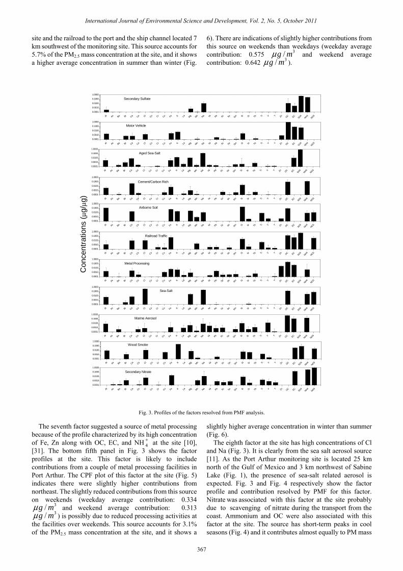
site and the railroad to the port and the ship channel located 7 km southwest of the monitoring site. This source accounts for 5.7% of the PM2.5 mass concentration at the site, and it shows a higher average concentration in summer than winter (Fig.

6). There are indications of slightly higher contributions from this source on weekends than weekdays (weekday average contribution: 0.575 3/g mμ and weekend average contribution: 0.642 3/g mμ ).

Al As Ba Br Ca Ce ClCo Cr Cu Fe K La Mg Mn Na Ni Pb Sc Se Sm Si Sr Tb Ti V Y Zn OC EC

SO4NH4

NO3

0.0001

0.0010

0.0100

0.1000

1.0000

Railroad Traffic


SO4NH4

NO3

0.0001

0.0010

0.0100

0.1000

1.0000

Secondary Nitrate


SO4NH4

NO3

0.0001

0.0010

0.0100

0.1000

1.0000

Sea-Salt

Al As Ba Br Ca Ce ClCo Cr Cu Fe K La Mg Mn Na Ni

Pb Sc Se Sm Si Sr Tb Ti V Y Zn OC ECSO4

NH4NO3

0.0001

0.0010

0.0100

0.1000

1.0000

Motor Vehicle


SO4NH4

NO3

0.0001

0.0010

0.0100

0.1000

1.0000

Marine Aerosol



NH4NO3

0.0001

0.0010

0.0100

0.1000

1.0000

Wood Smoke



NH4NO3

0.0001

0.0010

0.0100

0.1000

1.0000

Cement/Carbon Rich


SO4NH4

NO3

0.0001

0.0010

0.0100

0.1000

1.0000

Metal Processing


SO4NH4

NO3

0.0001

0.0010

0.0100

0.1000

1.0000

Secondary Sulfate



NH4NO3

0.0001

0.0010

0.0100

0.1000

1.0000

Aged Sea-Salt


SO4NH4

NO3

0.0001

0.0010

0.0100

0.1000

1.0000

Airborne Soil

Con

cent

ratio

ns (μ

g/μg

)

Fig. 3. Profiles of the factors resolved from PMF analysis.

The seventh factor suggested a source of metal processing

because of the profile characterized by its high concentration of Fe, Zn along with OC, EC, and NH 4

+ at the site [10], [31]. The bottom fifth panel in Fig. 3 shows the factor profiles at the site. This factor is likely to include contributions from a couple of metal processing facilities in Port Arthur. The CPF plot of this factor at the site (Fig. 5) indicates there were slightly higher contributions from northeast. The slightly reduced contributions from this source on weekends (weekday average contribution: 0.334

3/g mμ and weekend average contribution: 0.313 3/g mμ ) is possibly due to reduced processing activities at

the facilities over weekends. This source accounts for 3.1% of the PM2.5 mass concentration at the site, and it shows a

slightly higher average concentration in winter than summer (Fig. 6).

The eighth factor at the site has high concentrations of Cl and Na (Fig. 3). It is clearly from the sea salt aerosol source [11]. As the Port Arthur monitoring site is located 25 km north of the Gulf of Mexico and 3 km northwest of Sabine Lake (Fig. 1), the presence of sea-salt related aerosol is expected. Fig. 3 and Fig. 4 respectively show the factor profile and contribution resolved by PMF for this factor. Nitrate was associated with this factor at the site probably due to scavenging of nitrate during the transport from the coast. Ammonium and OC were also associated with this factor at the site. The source has short-term peaks in cool seasons (Fig. 4) and it contributes almost equally to PM mass


367

in summer and winter shown in Fig. 6. This source accounts for 3.0% of the PM2.5 mass concentration at the monitoring site. The CPF plot in Fig. 5 clearly shows the relationship of

this factor with wind directions from south. It indicates that this source is highly influenced by the monitoring site being in the proximity to the Gulf of Mexico.

0

6

12

8/30/2005

12/8/2005

3/18/2006

6/26/2006

10/4/2006

1/12/2007

4/22/2007

7/31/2007

11/8/2007

2/16/2008

5/26/20089/3/2008

12/12/2008

3/22/2009

6/30/20090

1

2

0

4

8

05

10152025

0

2

4

6

0

3

6

9

0

2

4

6

0

4

8

0

5

10

15

20

0

4

8

0

5

10

15

20

Railroad Traffic

Mas

s co

ncen

tratio

ns (μ

g/m

3 )

Secondary Nitrate

Sea-Salt

Motor Vehicle

Marine Aerosol

Wood Smoke

Cement/Carbon Rich

Metal Processing

Secondary Sulfate

Aged Sea-Salt

Airborne Soil

Fig. 4. Contributions by the factors resolved from PMF analysis.

The ninth factor was identified as marine aerosol related to the sea salt factor [11]. The bottom third panel in Fig. 3 shows the factor profile at the site. It has high concentration of Na, Si, V, OC, EC, and NH 4

+ . A small amount of Al, Cl, Fe, La, Mg, Ni, Pb, Sc, Sm, Sr, and Tb were also associated with this factor at the site. The content of Al, Cl, Fe, La, Na, Ni, Pb, Si, Sr, V, and high loading of OC, EC, NH 4

+ in the source suggests that this factor might have been influenced by marine shipping emissions along the Gulf Coast. Ship

traffic is increasingly recognized as a significant source for these trace metals in coastal areas. In Fig. 5, there are indications of higher concentrations at the site from the direction of southwest which is the direction towards the port and ship channel from the monitoring site. The source has some large peaks in spring (Fig. 4) and a slightly higher average concentration in winter than summer (Fig. 6). This source accounts for 2.8% of the PM2.5 mass concentration at the site.


368

The tenth factor was identified as wood smoke source which is characterized by Cl, K, EC, SO 2

4− , and NO 3

− [10], [22], [32]. A small amount of Al, Cu, Mg, Si, and Sr were also associated with this factor at the site. It contributes 2.4% to the PM2.5 mass concentration at the site. Fig. 3 shows the profile result and Fig. 4 shows the factor contribution result for this source at the site. The wood smoke probably comes from residential wood burning, local agricultural biomass burning, and occasional forest fires. The short-term peaks in spring and summer (Fig. 4) were probably due to forest fires,

and/or biomass burning from Central America. However, the short-term peaks in winter (Fig. 4) were probably due to residential wood burning. The CPF plot of this factor in Fig. 5 indicates that there were slightly higher contributions from northeast possibly because the business and residential areas in Port Arthur are located northeast of the monitoring site. The contributions from northeast were also likely influenced under less frequently northeasterly wind conditions in winter. This source has a slightly higher average concentration in winter than summer (Fig. 6).

0.5

1.00

30

60

90

120

150

180

210

240

270

300

330

0.5

1.0

0.5

1.00

30

60

90

120

150

180

210

240

270

300

330

0.5

1.0

0.25

0.50

0.75

1.000

30

60

90

120

150

180

210

240

270

300

330

0.25

0.50

0.75

1.00

0.25

0.50

0.75

1.000

30

60

90

120

150

180

210

240

270

300

330

0.25

0.50

0.75

1.00

0.25

0.50

0.75

1.000

30

60

90

120

150

180

210

240

270

300

330

0.25

0.50

0.75

1.00

0.25

0.50

0.75

1.000

30

60

90

120

150

180

210

240

270

300

330

0.25

0.50

0.75

1.00

0.50

0.75

1.000

30

60

90

120

150

180

210

240

270

300

330

0.50

0.75

1.00

0.25

0.50

0.75

1.000

30

60

90

120

150

180

210

240

270

300

330

0.25

0.50

0.75

1.00

0.50

0.75

1.000

30

60

90

120

150

180

210

240

270

300

330

0.50

0.75

1.00

0.25

0.50

0.75

1.000

30

60

90

120

150

180

210

240

270

300

330

0.25

0.50

0.75

1.00

0.50

0.75

1.000

30

60

90

120

150

180

210

240

270

300

330

0.50

0.75

1.00

Railroad Traffic

Secondary Nitrate

Sea Salt

Motor Vehicle

Marine Aerosol

Wood Smoke

Cement/Carbon Rich

Metal Processing

Secondary Sulfate Aged Sea Salt

Airborne Soil

Fig. 5. CPF plots for the highest 25% of the mass contributions.


369

0

1

2

3

4

5

Secondary nitrate

Wood smoke

Marine aerosolSea salt

Metal processing

Railroad tra

ffic

Airborne soil

Cement/carbon rich

Motor vehicle

Aged sea salt

Aver

age

Con

tribu

tions

(μg/

m3 )

Summer Winter

Secondary sulfate

Fig. 6. Comparison of summer (April-September) versus winter

(October-March) contributions for each source. The eleventh factor resolved at the site mainly consists of

ammonium and nitrate. The nitrate-rich secondary aerosol is identified by its high concentrations of NO 3

− and NH 4+ . Fig.

3 shows the profile result and Fig. 4 shows the factor contribution result for this source. EC and a small amount of trace metals were also associated with this factor possibly from the transported metallic aerosol. This source includes NH 4

+ concentration that becomes associated with the secondary nitrate aerosol in the atmosphere. Molar ratio of ammonium to nitrate for this factor was 1.3 (0.07172/18:0.19739/62) at the site. Because of the possible evaporation of ammonium during sample analysis and/or the uncertainty of the PMF estimate, nitrate is probably present mainly as ammonium nitrate at the receptor site. Nitrate is formed in the atmosphere mostly through the oxidation of NOx depending on ambient temperature, relative humidity, and the presence of ammonia [22]. It has short-term peaks and higher trend in cool seasons possibly indicating that low temperature and high humidity foster the formation of nitrate aerosol in the region as discussed in the study for Atlanta [10] and three northeastern US cities [25]. Fig. 6 shows this source contributed more to the PM mass concentration in winter than summer which is consistent with the preceding discussion of nitrate formation likely in cool season. In the CPF plot of this factor at the site (Fig. 5), the higher contributions from southeast indicate that the nitrate aerosol was possibly influenced by the sources along the Gulf Coast under prevailing flow from the south, in particular, the refineries located in south of the monitoring site. The source accounts for 1.9% of the PM2.5 mass concentration at the site.

IV. CONCLUSION An air quality study has been carried out to identify the

sources of particulate pollutants at an EPA monitoring site in Texas, namely, the Port Arthur site located in Golden Triangle of Texas with about 30 km southeast of Interstate Highway 10. This site has average annual PM concentration of 11.28 3/g mμ which is below the National Ambient Air Quality Standards of 15 3/g mμ for PM. In this study, the collected PM2.5 compositional data at the monitoring site were analyzed using PMF for source attribution. The PMF

effectively identified eleven possible source-related factors for PM2.5. The estimated source contributions for the eleven factors at the site were obtained from the PMF analysis.

Sulfate-rich secondary aerosol extracted by PMF had the highest contribution to the PM2.5 mass in the region and accounted for almost 32% of the total concentration at the site. Sulfate and nitrate mainly exist as ammonium sulfate and ammonium nitrate at the receptor site. The airborne soil factor has high source contribution peaks during the summer likely reflecting the intercontinental dust transport. The sea salt factor is clearly seen at the site from the Gulf of Mexico. The aged sea-salt aerosol was originated from sea salt aerosol; however, it was separately identified because of the chloride loss during chemical reactions in the atmosphere. A couple of metal processing facilities in Port Arthur are clearly suggested of being related to the source of metal processing. The marine aerosol is mainly influenced by ship traffic at the ship channel and the port. Sulfate, airborne soil, nitrate are likely to be regional factors; however, motor vehicle, cement/carbon-rich, railroad traffic, metal processing, marine aerosol, and wood smoke are likely to be local factors.

ACKNOWLEDGMENT This study was supported in part by the US EPA through

project R-07-0159. The authors wish to thank Professor P.K. Hopke of Clarkson University for helpful e-mail communica- tions. The result of this research represents only the authors’ assessments and does not reflect the funding agency’s views on the air quality issues in this region.

REFERENCES [1] P. K. Hopke, Receptor Modeling in Environmental Chemistry, New

York: John Wiley & Sons, 1985, ch. 1, 5, and 6. [2] P. K. Hopke, Receptor Modeling for Air Quality Management,

Amsterdam: Elsevier Science, 1991, ch. 1 and 5. [3] P. Paatero, “Least squares formulation of robust, non-negative factor

analysis,” Chemomet. Intell. Lab. Syst., vol. 37, pp. 23-35, 1997. [4] P. Paatero and U. Tapper, “Analysis of different modes of factor

analysis as least squares fit problems,” Chemomet. Intell. Lab. Syst., vol. 18, pp. 183-194, 1993.

[5] P. Paatero and U. Tapper, “Positive matrix factorization: a non-negative factor models with optimal utilization of error estimates of data values,” Environmetrics, vol. 5, pp. 111-126, 1994.

[6] P. Anttila, P. Paatero, U. Tapper, and O. Järvinen, “Source identification of bulk wet deposition in Finland by positive matrix factorization,” Atmos. Environ., vol. 29, pp. 1705-1718, 1995.

[7] W. Chueinta, P. K. Hopke, P. Paatero, “Investigation of sources of atmospheric aerosol at urban and suburban residential areas in Thailand by positive matrix factorization,” Atmos. Environ., vol. 34, pp. 3319-3329, 2000.

[8] S. Juntto and P. Paatero, “Analysis of daily precipitation data by positive matrix factorization,” Environmetrics, vol. 5, pp. 127-144, 1994.

[9] E. Kim, P. K. Hopke, and E. S. Edgerton, “Source identification of Atlanta aerosol by positive matrix factorization,” J. Air Waste Manage. Assoc., vol. 53, pp. 731-739, 2003.

[10] E. Kim, P. K. Hopke, and E. S. Edgerton, “Improving source identification of Atlanta aerosol using temperature resolved carbon fractions in positive matrix factorization,” Atmos. Environ., vol. 38, pp. 3349-3362, 2004.

[11] E. Lee, C. K. Chan, and P. Paatero, “Application of positive matrix factorization in source apportionment of particulate pollutants in Hong Kong,” Atmos. Environ., vol. 33, pp. 3201-3212, 1999.

[12] K. G. Paterson, J. L. Sagady, D. L. Hooper, S. B. Bertman, M. A. Carroll, and P. B. Shepson, “Analysis of air quality data using positive


370

matrix factorization,” Environ. Sci. Technol., vol. 33, pp. 635-641, 1999.

[13] A. V. Polissar, P. K. Hopke, W. C. Malm, and J. F. Sisler, “The ratio of aerosol optical absorption coefficients to sulfur concentrations, as an indicator of smoke from forest fires when sampling in polar regions,” Atmos. Environ., vol. 30, pp. 1147-1157, 1996.

[14] A. V. Polissar, P. K. Hopke, P. Paatero, W. C. Malm, and J. F. Sisler, “Atmospheric aerosol over Alaska: 2. Elemental composition and sources,” J. Geophys. Res., vol. 103, pp. 19045-19057, 1998.

[15] A. V. Polissar, P. K. Hopke, P. Paatero, Y. J. Kaufman, D. K. Hall, B. A. Bodhaine, E. G. Dutton, and J. M. Harris, “The aerosol at Barrow, Alaska: long-term trends and source locations,” Atmos. Environ., vol. 33, pp. 2441-2458, 1999.

[16] A. V. Polissar, P. K. Hopke, and R. L. Poirot, “Atmospheric aerosol over Vermont: chemical composition and sources,” Environ. Sci. Technol., vol. 35, pp. 4604-4621, 2001.

[17] Y. L. Xie, P. K. Hopke, P. Paatero, L. A. Barrie, and S. M. Li, “Identification of source nature and seasonal variations of Arctic aerosol by positive matrix factorization,” J. Atmos. Sci., vol. 56, pp. 249-260, 1999.

[18] P. Chiou, W. Tang, C. J. Lin, H. W. Chu, and T. C. Ho, “Atmospheric aerosol over a southeastern region of Texas: chemical composition and possible sources,” Environ. Model. Assess., vol. 14, pp. 333-350, 2009.

[19] P. Chiou, W. Tang, C. J. Lin, H. W. Chu, R. Tadmor, and T. C. Ho, “Atmospheric aerosol over a southwestern region of Texas,” Environ. Model. Assess., vol. 14, pp. 645-659, 2009.

[20] P. Chiou, J. Shah, C. J. Lin, R. Tadmor, H. W. Chu, and T. C. Ho, “Source identification of Houston aerosol with carbon fractions in positive matrix factorization,” Int. J. Environ. Develop., vol. 7, no. 1, pp. 135-152, 2010.

[21] D. A. Hansen, E. S. Edgerton, B. E. Hartsell, J. J. Jansen, N. Kandasamy, G. M. Hidy, and C. L. Blanchard, “The Southeastern aerosol research and characterization study: Part 1 – overview,” J. Air Waste Manage. Assoc., vol. 53, pp. 1460-1471, 2003.

[22] W. Liu, Y. H. Wang, R. Armistead, and E. S. Edgerton, “Atmospheric aerosol over two urban-rural pairs in the southeastern United States:

chemical composition and possible sources,” Atmos. Environ., vol. 39, pp. 4453-4470, 2005.

[23] Z. Ramadan, X. H. Song, and P. K. Hopke, “Identification of sources of Phoenix aerosol by positive matrix factorization,” J. Air Waste Manage. Assoc., vol. 50, pp. 1308-1320, 2000.

[24] Z. Ramadan, B. Eickhout, X. H. Song, L. M. C. Buydens, and P. K. Hopke, “Comparison of positive matrix factorization and multilinear engine for the source apportionment of particulate pollutants,” Chemomet. Intell. Lab. Syst., vol. 66, pp. 15-28, 2003.

[25] X. H. Song, A. V. Polissar, and P. K. Hopke, “Sources of fine particle composition in the northeastern US,” Atmos. Environ., vol. 35, pp. 5277-5286, 2001.

[26] M. Zheng, G. R. Cass, J. J. Schauer, and E. S. Edgerton, “Source apportionment of PM2.5 in the southeastern United States using solvent-extractable organic compounds as tracers,” Environ. Sci. Technol., vol. 36, pp. 2361-2371, 2002.

[27] P. J. Huber, Robust Statistics, New York: John Wiley, 1981, ch.7, pp. 162-164.

[28] L. L. Ashbaugh, W. C. Malm, and W. Z. Sadeh, “A residence time probability analysis of sulfur concentrations at Grand Canyon National Park,” Atmos. Environ., vol. 19, pp. 1263-1270, 1985.

[29] E. Yakovleva, P. K. Hopke, and L. Wallace, “Receptor modeling assessment of PTEAM data,” Environ. Sci. Technol., vol. 33, pp. 3645-3652, 1999.

[30] B. Efron and R. L. Tibshirani, An Introduction to the Bootstrap. London: Chapman and Hall, 1993, ch. 13, pp. 168-177.

[31] SPECIATE Version 3.2, US Environmental Protection Agency, Research Triangle Park, NC, 2002.

[32] J. G. Watson, J. C. Chow, and J. E. Houck, “PM2.5 chemical source profiles for vehicle exhaust, vegetative burning, geological material, and coal burning in northwestern Colorado during 1995,” Chemosphere, vol. 43, pp. 1141-1151, 2001.

[33] J. M. Prospero, “African dust in America,” Geotimes, pp. 24-27, Nov. 2001.


371

Documents

Source Identification and Apportionment of Atmospheric ...ijesd.org/papers/152-D579.pdf · Paul Chiou, Wei Tang, Jalpa Shah, Rafael Tadmor, and T.C. Ho International Journal of Environmental