Source effects on strong-motion records and resolving …web.gps.caltech.edu/~ampuero/tmp/SrcInv/Iid93_source_inversion.pdf · We find that the physical wave is a key concept for

Tectonophysics, 218 (1993) 179-193 Elsevier Science Publishers B.V., Amsterdam

179

Source effects on strong-motion records and resolving power of strong-motion arrays for source inversion

Masahiro Iida

Earthquake Research Institute, University of Tokyo, Tokyo 113, Japan

(Received June 4,199l; revised version accepted January 10,1992)

ABSTRACT

Iida, M., 1993. Source effects on strong-motion records and resolving power of strong-motion arrays for source inversion. In: F. Lund (Editor), New Horizons in Strong Motion: Seismic Studies and Engineering Practice. ~eefo~~~y~~cs, 218: 179-193.

Source effects are dominant in near-source strong-motion seismograms, even in the high-frequency range, and source inversion is the most powerful tool for investigating source effects. First, source effects that are closely related to damage and intensity patterns are briefly shown. Large inconsistencies have been seen among source inversion results. The cause seems to come mainly from insufficient station distribution for earthquake source studies. However, the deployment strategy of strong-motion seismographs has been only poorly explored.

Secondly, three kinds of simulations conducted for the last several years are shown, in order to indicate the vulnerability of the resolving power of strong-motion arrays to a source inversion. The simulations are: (1) to obtain a relationship between the accuracy of the source inversion and fault-array parameters; (2) to present the optimum array geometry for the source inversion; and (3) to describe the relative significance of various seismic waves in the source inversion.

Thirdly, basic guidelines on strong-motion array layout for source inversion are provided and general comments are given on actual source inversion methods. We find that the physical wave is a key concept for unde~tand~g the optimum array con~guration and for choosing the most pertinent inversion method. Frequency consideration, which is a remaining problem, is required to decide the best inversion method and the best array Iayout. We can design sting-motion array for source inversion on the condition that frequency contents, fault mechanism, the spatial resolution and the inversion accuracy are prescribed.

Introduction

Understanding the nature of high-frequency, strong seismic ground motion is a crucial problem in both seismology and earthquake engineering. Although the local effects of strong-motion have been verified by numerous studies, aImost no study has been made investigating source effects that are closely related to damage and intensity patternsJin the high-frequency range. The most likely reason is a lack of well-instrumented earth- quakes a&lable for detailed source studies.

Correspondence to: M. Iida, Earthquake Research Institute, University of Tokyo, Tokyo 113, Japan.

Source inversion is the most powerful tool for investigating source effects. However, large inconsistencies have been seen among source inversion results. A typical inconsistency was found in the results for the 1979 Imperial Valley earthquake (e.g., Olson and Apsel, 1982; Hartzell and Heaton, 1983; Arch&eta, 1984). The differences in the results seem to come mainly from the differences in the model construction and insufficient station distribution for earthquake source studies. Inversion results should not be affected by the station distribution.

The deployment strategy of strong-motion seismographs has been only poorly explored. We have realized only empirically that source inversion results are strongly influenced by the num-

HO-1951/93/$~.~ 0 1993 - Elsevier Science Publishers B.V. Ah rights reserved

180 M. IIDA

ber of stations and the array configuration. At the International Workshop on Strong-Motion Earth- quake Instrumented Arrays held in Honolulu, Hawaii in 1978 (Iwan, 19781, a preferable array configuration was proposed on the basis of empirical judgement. That was the first proposal of an advantageous distribution of strong-motion array stations.

Three different array networks for source mechanism and wave propagation studies (de- pending on the source type), have been presented

: :: . *.:. . . ..-.‘..... :.*.:.::..-.

LKrn Map View Fault_

Map View I

(Fig. 1). First, a comb-shaped array, comprising approximately 100-200 instruments, is recom- mend for a strike-slip source mechanism, as shown in Figure la. About half of the instruments are aligned at an average spacing of approximately 10 km along a line parallel to the fault strike on one side of the fault (because of the symmetry of the radiation patterns about the fault strike). The instruments contribute to the identification of the relative locations of constituent multiple events during a fault rupture process. The remaining

Intensified Station

Array Station Spacing: 2-10km

(b)

Array Station

Fig. 1. Array configurations for source mechanism and wave propagation studies recommended at the 1978 International Workshop

on Strong-Motion Earthquake Instrument Arrays. (a) Strike-slip. (b) Dip-slip. Cc) Subduction thrust fault (after Iwan, 1978).

STRONG-MOTION: SOURCE EFFECTS AND THE RESOLVING POWER OF ARRAYS 181

instruments are arranged along a few legs extend- ing perpendicular to the fault strike. These legs (which have a length of 40-100 km) extend lin- early and are primarily available for the study of path effects. They also help in aiding in the discrimination of the multiple events.

Secondly, a two-dimensional array configuration, comprising appro~mately 100 instruments with a spacing of 2-10 km, is recommended for a dip-slip source mechanism (Fig. lb). The instrument placement is intended to discover if the

acceleration on the hanging wall is significantly different from that on the foot wall, and if there is signifi~ntly higher acceleration along the direction of strike or along the direction of propagation of the fault rupture. Thirdly, a linear or two-dimensional, narrow-band array, consisting of approximately SO-150 instruments, with an average spacing of 20 km, is recommended for a subduction thrust source mechanism (Fig. 1~). The instrument spacing is determined by the fault depth of the damaging shallow event. However,

Bandpassed North-Soufh Gmpmnf of Peak Vekxity fcmkec) W

/\’ \’ - &PASADENA

Fig. 2. Regional modified Mercalli intensity iso-seismats in the Los Angeles area for the earthquake of October 1, 1987. Circles = the center of the census traces surveyed; circled star = the main shock epicenter (after Leyendecker et al., 1988). Insert: Predicted peak velocities (cm/s) for model (b) of Figure 3 in the bandpass 0.2-3.0 Hz. Values contoured are the peak whole record

velocities for the north-south component of motion; triangles = stations used.

182 M. IIDA

to date, no quantitative analysis has yet been carried out on how the array stations should be deployed, and which types of seismic waves should be analyzed.

Only few attempts have been made to estimate effects of station array. Spudich and Oppen- heimer (1986) measured the resolving power of a hypothetical, differential seismograph array for high-frequency ground motions (> 1 Hz) by per- forming frequency-wavenumber analysis and ray tracing. Olson and Anderson (1988) showed that the assumed solution was not recovered by their frequency-domain inversion method with a minimum norm to obtain a unique solution, and that the quality of recovery was dependent upon the station array. Iida et al. (1988) represented the effects of array configuration by a single parameter on the basis of their method (Miyatake et aI., 1986). Although these studies used Green’s functions that were too simple, the significance of good strong-motion array was undoubtedly demonstrated.

I am developing two sorts of studies using a more realistic Green’s function in order to indicate station-array effects. One is to evaluate the influence of array parameters, such as the number of stations and the azimuthal coverage of the array, and the other is to evaluate the influence of array configuration, which is difficult to pa- rameterize. These studies are also applied to existing arrays. Since the quality of a station array should be associated with seismic waves to be analyzed, the relative significance of various seismic waves in the source inversion is examined. Although some of these studies have been re- cently published separately, the joint interpretation is very important in order to gain a general insight into the effectiveness of strong-motion

arrays. In this article we first summarize a study in

which source effects on strong-motion records were demonstrated, for one of the best instrumented ea~hquakes to date, using a source inversion method. Secondly, three kinds of simulations are described in order to indicate the vulnerability of the resolving power of strong-motion arrays for a source inversion. Finally, a joint interpretation of these studies is made and it is shown that

we can reasonably design a strong-motion array for source inversion under a given condition.

Source effects on strong motion records

Here one example is given which demonstrates the source effects on strong-motion records using one of the best instrumented earthquake to date (Hartzell and Iida, 1990). Seventeen near-source, strong-motion records for the 1987 Whittier Nar- rows, California, earthquake, with a local magni- tude of 5.9, are inverted to obtain the history of slip. The good station pattern, which forms a 360” azimuthal coverage of the source, is expected to give good resolution (Iida et al., 1988; Iida, 1990) (Fig. 2). Band-pass filtered velocity records from 0.2 to 3.0 Hz are used. This frequency range is important in earthquake engineering and is re- sponsible for much of an earthquake’s damage and intensity.

Figure 3 shows the contours of slip (in centimeters) for three inversion models. The similar- ity of the slip distribution in different rupture modes should be noted. The results show a complex rupture process within a small source vol- ume. There is a good fit between the synthetic and recorded waveforms in both shape and amplitude, especially in the earlier parts of the records including the Iarge-amplitude sections. This suggests that the inversion was very success- ful (Fig. 4). The ground motion in the epicentral region is predicted based upon the inferred distribution of slip from our inversion, The results are shown on the same scale in Figure 2, where peak velocities are contoured. This result is helpful in providing a good interpretation of the unusual intensity and damage patterns of this earthquake (Leyendecker et al., 1988). We conclude that the ground motion can be explained by considering the source effects, coupled with the same aver- aged propagation path effects to each strong- motion station.

Resolving power of strong-motion arrays for source inversion

Above we confirmed that strong-motion seismograms were heavily controlled by source ef-

fects. Another fact is that the differences in the model construction did not produce remarkable differences in the results. This means that the inconsistencies recognized among source inversion resuIts are primarily due to the insufficient resolving power of strong-motion arrays. After reviewing our method the dependence of the accuracy (the uncertainty) of an inversion SOIU-

E W

1oiW 1 1 1 1 ' ( ' 123456789

Distance Along Strike (km)

( > a

tion on the array geometry is investigated and the contribution of various seismic waves to the accuracy of the inversion solution is measured.

Methods

Since the method has been explained else- where (e.g., Iida et al., 199Ob), only a brief sum-

L J

Distance Alolg Strike (km)

(b)

Distance Along Strike (km)

( ) C Fig. 3. Contours of slip (in centimeters) for three inversion models. (a) Each subfault ruptures once at a constant rupture velocity of

2.5 km/s. (b) Each subfault is allowed to rupture twice to allow for a more complex source-time function. The rupture velocity is

fixed at 2.5 km/s. (c) Each subfault ruptures once, but the rupture velocity is not fixed, and the rupture times for each subfault are

free to vary.

184 M. IIDA

mary is given here. Wolberg’s (1967) prediction analysis was used to calculate the accuracy of a waveform solution from errors contained in data by using a principle of error propagation. Most of the current source inversion studies deaI with a detailed history of rupturing on a fault. We di- vided the entire fault into many subfaults and used a displacement waveform representation for each subfault. A complete Green’s function in a semi-infinite elastic space was used. A common, simple source-time function was assumed for each subfault. The seismic moment and the rup-

ture onset time for each subfault were chosen as unknown parameters. The unknown parameters were determined using a least-squares criterion. Uncertainties were assumed for several known variables. We estimated the accuracy of the source inversion, u, from the maximum standard deviation of the seismic moments for all subfaults, normalized by the seismic moment.

The theoretical waveform is a function of known and unknown parameters. The known parameters, whose uncertainties are taken into account (the dip angle, the strike direction, the slip

FRS SWA OBP

3* 0 360” 12.7 17.1 17.1 192

+_---_ l5.o -g 12.3

16.5

ECP DOW GVR

Fig. 4. Comparison of the observed velocity records (first trace) with the synthetic records for model in Fig. 3b (model L18, second

trace) and model in Fig. 3c (model NL 22, third trace) for six different stations.


angle, the wave amplitude and the arrival time) are denoted by xP (p = 1,. , . , N,). The unknown parameters, the seismic moment and rupture onset time for each subfault are denoted by a, (i= 1 ,..., NJ. The wave amplitude for the jth time point at the kth station is expressed as

U“(tj) =fjk(Xikj,. . .y “Npkj; al,. . .T a,)* TWO residuals, Rukj and RxPkj are defined as the differences between the observed and calculated values:

Rukj = U“( tj) - u”(t,) (1)

RYpkj = Xpkj - XPkj (2)

where Uk(fj) and Xpkj (p = 1,. . . , ZV,) are the observed wave amplitude and the true value for the known parameter, respectively.

The least-squares method is used to determine the values of the unknown parameters, a, (i = 1 ,..., NJ, which minimize the weighted sum of the squares of the residuals, S:

s = c c WUkjRU;j + c wx,kjfh;kj

k j (

NP

!

(3) P

where wUkj = I/uu:~ and Wxpkj = I/cTx~,~;

auki = the standard deviation of the wave amplitude; and axPkj = the standard deviation of the known parameter.

In general, the solution for the least-squares problem is obtained by solving normal equations in a matrix form. Following Wolberg’s (1967) prediction analysis, however, the uncertainty of the ith unknown parameter, aai can be estimated by calculating the inverse of a matrix. In this case it is unnecessary to solve the actual normal equations. Three sorts of simulations are shown below.

Relationship between the accuracy of source inversion and fault-array parameters (1st simulation)

A systematic analysis was carried out to obtain a relationship between the accuracy of the source inversion and fault-array parameters (Iida et al., 1990b). Strike-slip and dip-slip faults were assumed to be located at the center of a circular array (Fig. 5). Several fault-array parameters were

T Ne=l8 0.5

JL @ = 0.5

+I* Fig. 5. Geometrical arrangement of fault planes and array

stations. Two kinds of faults are located at the center of an

array: a pure strike-slip fault with a dip angle, S = 90” and a

pure dip-slip fault with 6 = 30”. All the distances are normal-

ized by the fault length.

separately varied and their effects on the accuracy of the source inversion were evaluated.

Fault parameters

Five parameters were considered: (1) the number of subfaults, N,; (2) the aspect ratio, @; (3) the dip angle, 6; (4) the fault depth, h; and (5) the rupture mode. We found that the normalized uncertainty, C, was roughly proportional to NC2, independent of the fault mechanism. Depth resolution was worse than the resolution in the horizontal direction. The uncertainty did not depend much on the dip angle, the fault depth and the rupture mode.

Array parameters

Array parameters are important because they can be controlled. Four parameters were exam-

1% M. IIDA

ined: (1) the number of stations, N,; (2) the array radius, R; (3) the azimuthal coverage of the source, 4; and (4) the components of the seismograms. The effects of the array parameters are summarized in Figure 6.

The uncertainty, CT, is found to obey roughly an inverse root dependence on NS (Fig. 6a). To-

gether with the number of subfaults, N,, the relationship, cr CY N,*/N,‘/*, suggests that numerous stations are required to analyze the detailed rupturing process. Figure 6b shows that the inversion uncertainty reaches a minimum when the array radius, R, is around 0.75-2.0 times the fault length. CJ a c#-’ holds approximately in the case

u

‘“1 (a)

I

0.1

0.0 I

l \

Strike Slip Fmlt

Dip Slip Fault

I 5 IO 50

Ns

cl-

5

I

(b)

Strike SIip Fault

l

Components

0 Strike Slip Fault

0 Dip Slip Fault

Fig. 6. Relationship between the inversion uncertainty, (T, and array parameters. (a) The number of the stations, N,. (b) The array

radius, R. (c) The azimuthal coverage, 4, Case A = rupture propagating towards the array; case B = rupture moving away from the

array. (d) The components of the seismograms. 2 = component parallel to the fault strike; 2 = horizontal component perpendicular

to the fault strike; 3 = vertical component.

STRONG-MOTION: SOURCE EFFECTS AND THE RESOLVING’POWER OF ARRAYS 187

Surface station installation zone

I

0 0 0 0

b) Ns=4

0 0 0 0 0 0 0 0

c) Ns=8

Is 8 I 8 8 01 d) Ns=18

I I

\ Fault area

Fig. 7. Geometrical arrangement of fault and array stations for a simulation on an offshore subduction thrust. A pure dip-slip fault

with a dip angle, 6 = 30”, which is the same as that in Fig. 5, is assumed. The numbers of surface stations and ocean bottom

stations, N, and N, are varied separately to estimate their influence. The distribution in the surface stations is fixed, based upon

the number of surface stations, N,. and forms a line or a rectangular grid. Several patterns of ocean bottom stations are tested for

each pair of N, and N,,.

where N, is kept proportional to C#J (Fig. 6~). Note that u a NSP1/* holds when the azimuthal coverage is unchanged. Thus, the relationship aa@’ under the condition of u a IV, implies a remarkable contribution from the azimuthal cov-

erage. In Figure 6c, the relationship is determined by the case where the rupture direction is considered disadvantageous for the station array (i.e., the rupture propagates towards the station array, case A). Figure 6d shows that the horizon-

5r

5 10 15 20 Surface station Ns installation zone

CI) No=1 b) No=2 c) No=4 d) No=4 (&=2.4.8) (Ns=2.4.8) (Ns=4) (Ns=~)

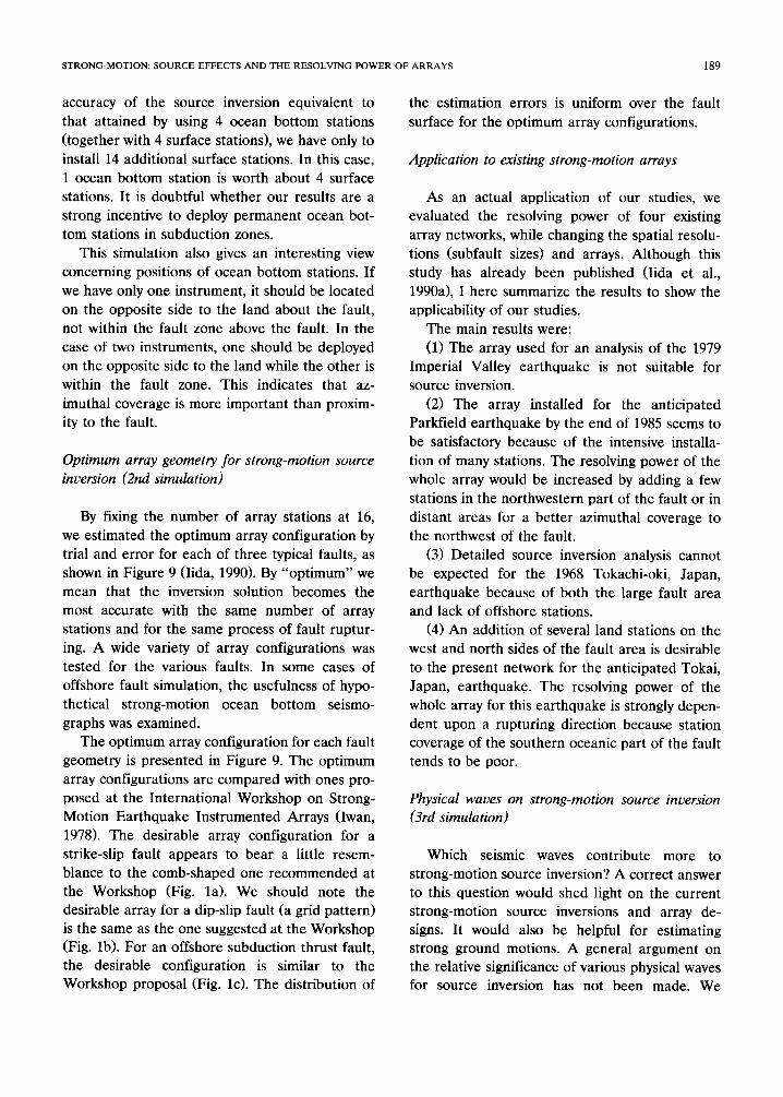
Fig. 8. Relationship among the inversion uncertainty, (T, and the numbers of surface stations and ocean bottom stations, N, and N,.

The best positions of ocean bottom stations are depicted for each pair of N, and N,. We find that, when 1 or 2 ocean bottom

seismographs are installed, the locations are not dependent on the number of surface stations, N,; whereas the locations are

changed according to N, in the case of 4 ocean bottom seismographs.

188

tal component parallel to the fault strike tends to contribute to a strike-slip fault and the vertical component to a dip-slip fault.

Subduction thrust simulation

By conducting a test on the relative value of ocean bottom seismographs and surface seismographs for studying the rupture of a subduction event, we attempted to demonstrate or refute their necessity. Up to now, no quantitative argu- ments on whether strong-motion ocean bottom seismographs are worth installing have been made. At present, a semi-pe~anent, strong- motion ocean bottom seismograph does not exist, although temporary networks of strong-motion ocean bottom seismograph systems are being de- veloped. Since 1978, relatively low cost seismic stations for measuring strong ground motion on the ocean bottom have been tested (Steinmetz et al., 1979; 1981). These experiments indicate that an ocean bottom station is capable of recording ground accelerations up to about 1.0 g in the

b 45km

Depth 3.0

(km1 8.3

1 1 10.6km

r3.c

6 =45”lnorth-dtppingi h=3km

(b)

M. IIDA

0.1-10 Hz frequency band, with good reliability in most cohesive type soil conditions.

For this simulation, the fault and array geometry shown in Figure 7 was used. The numbers of surface stations and ocean bottom stations, N, and N, were varied separately to estimate their influence. The positions of the surface stations were fixed, as illustrated in Figure ‘7. Several patterns of ocean bottom stations were tested for each pair of N, and N,. They were intended to determine the best position for a combination of stations.

The effects of the increasing numbers of surface stations and ocean bottom stations on the inversion uncertainty are shown in Figure 8. In- terestingly, the inversion uncertainty does not appear to saturate as the number of surface stations is increased in the absence of ocean bottom stations. The graph suggests that the effects of ocean bottom stations are not very dramatic. For example, even if we increase the number from 1 to 2 or from 2 to 4, a large drop in the inversion uncertainty is not seen. In order to recover the

_-..

‘-7 __~_: ’ lOOkIn SOkm a i&l

(Cl)

Land

sea

(b) (c2)

Fig. 9. Fault geometries used for investigating effects of array confjgurations on the source inversion (side views) and the optimum array configuration obtained for each of 3 fault geometries. (a) Strike-slip. (b) Dip-slip. (c) Subduction thrust fault; case

cl = without and c2 = with strong-motion ocean bottom seismograms.


accuracy of the source inversion equivalent to that attained by using 4 ocean bottom stations (together with 4 surface stations), we have only to install 14 additional surface stations. In this case, 1 ocean bottom station is worth about 4 surface stations. It is doubtful whether our results are a strong incentive to deploy permanent ocean bottom stations in subduction zones.

This simulation also gives an interesting view concerning positions of ocean bottom stations. If we have only one instrument, it should be located on the opposite side to the land about the fault, not within the fault zone above the fault. In the case of two instruments, one should be deployed on the opposite side to the land while the other is within the fault zone. This indicates that azimuthal coverage is more important than proxim- ity to the fault.

Optimum array geometry for strong-motion source inversion (2nd simulation)

By fixing the number of array stations at 16, we estimated the optimum array configuration by trial and error for each of three typical faults, as shown in Figure 9 (Iida, 1990). By “optimum” we mean that the inversion solution becomes the most accurate with the same number of array stations and for the same process of fault rupturing. A wide variety of array configurations was tested for the various faults. In some cases of offshore fault simulation, the usefulness of hypothetical strong-motion ocean bottom seismographs was examined.

The optimum array configuration for each fault geometry is presented in Figure 9. The optimum array configurations are compared with ones proposed at the International Workshop on Strong- Motion Earthquake Instrumented Arrays (Iwan, 1978). The desirable array configuration for a strike-slip fault appears to bear a little resem- blance to the comb-shaped one recommended at the Workshop (Fig. la). We should note the desirable array for a dip-slip fault (a grid pattern) is the same as the one suggested at the Workshop (Fig. lb). For an offshore subduction thrust fault, the desirable configuration is similar to the Workshop proposal (Fig. 1~). The distribution of

the estimation errors is uniform over the fault surface for the optimum array configurations.

Application to existing strong-motion arrays

As an actual application of our studies, we evaluated the resolving power of four existing array networks, while changing the spatial resolu- tions (subfault sizes) and arrays. Although this study has already been published (Iida et al., 1990a), I here summarize the results to show the applicability of our studies.

The main results were: (11 The array used for an analysis of the 1979

Imperial Valley earthquake is not suitable for source inversion.

(2) The array installed for the anticipated Parkfield earthquake by the end of 1985 seems to be satisfactory because of the intensive installation of many stations. The resolving power of the whole array would be increased by adding a few stations in the northwestern part of the fault or in distant areas for a better azimuthal coverage to the northwest of the fault.

(3) Detailed source inversion analysis cannot be expected for the 1968 Tokachi-oki, Japan, earthquake because of both the large fault area and lack of offshore stations.

(4) An addition of several land stations on the west and north sides of the fault area is desirable to the present network for the anticipated Tokai, Japan, earthquake. The resolving power of the whole array for this earthquake is strongly dependent upon a rupturing direction because station coverage of the southern oceanic part of the fault tends to be poor.

Physical waves on strong-motion source inversion (3rd simulation)

Which seismic waves contribute more to strong-motion source inversion? A correct answer to this question would shed light on the current strong-motion source inversions and array de- signs. It would also be helpful for estimating strong ground motions. A general argument on the relative significance of various physical waves for source inversion has not been made. We

190 M. IIDA

attempt to give an answer by measuring the dete- rioration in the accuracy of the source inversion when various wave types are removed from the problem.

There seem to be two major differences between the real structure of the Earth and the homogeneous half-space used in our study: (1) the half-space has no Love waves; and (2) the half-space model may not be a good one in terms of the body waves that leave the source in a downwards direction and are observed at distant stations. If we can understand the physical pro- cesses that produce our results, we may be able to solve these problems. It would be very helpful to show which physical waves contribute more to the accuracy of the source inversion in the half- space model. It should be noted that, whereas an increase in the information about the source contained in the waveform decreases the uncertainty of the solution, it simultaneously complicates the waveform by interference with different phases and results in an increase in the uncertainty.

Dip angle and fault depth

Two factors on physical waves which may be worth examining are dip angle and fault depth. Dip angle is related to the relative separation in arrival times between seismic waves radiated from subfaults, while a shallow fault depth causes a preponderance of surface waves. The fault-array layout used (which is very similar to that in Fig- ure 5), is shown in Figure 10. Three stations are installed near the fault in order to emphasize the near-field terms. The three types of fault geometries used are summarized in Table 1. We can derive the effects of phase interference due to the relative separation in arrival times between seismic waves, using:

4 t,, - tsi PI== t:-

i-1 s

where tri and tsi are the arrival times of the latest Rayleigh wave and the earliest S wave observed at the ith station. The calculated values are listed in Table 1. The average depth of faults is normalized by the fault length. A small PI means large

K=2

Ne=8

(9 =0.5

t---l-i Fig. 10. Geometrical arrangement of fault planes and array stations for studying effects of phase interference and source depth. Three sorts of faults summarized in Table 1 are used.

All the distances are normalized by the fault length.

phase interference due to fault geometry (i.e., dip angle). The first fault plane, with a 90” dip, will produce more severe phase interference than the other two planes. In addition, we will demonstrate the effects of surface wave dominance due to different source depths, using the second and third fault planes. The types of physical waves used at each station are shown in Figure 11. The same ten cases were tested for each of the three fault planes. Important comparisons are those of

TABLE I

Three types of fault geometries used to study effects of various physical waves

Type Slip direction Dip angle Average depth

0 of fault PI

[ll Strike-slip 90 0.35 1.02

121 Dip-slip 30 0.225 1.17

t31 Dip-slip 30 0.35 1.13

Average depth of fault is normalized by fault length. Parame- ter, PI is introduced to measure phase interference due to fault geometry. See text for definition.


cases (1) and (3) for surface waves, cases (2) and (5) for near-field terms, and cases (4) and (10) for far-field terms.

The accuracy of the source inversion is summarized in Figure 11. At first glance, we find that results for the fault planes of [2] and [3] show a different trend from a result for the fault plane of [l]. In the inclined dip-slip fault planes, primarily surface waves at distant stations contribute to the source inversion. Secondly, far-field terms are a main contributor in the absence of surface waves at distant stations, whereas near-field terms are not. Use of the shallower fault, [2], identical in geometry to the deeper fault, [3], shows that a predominance of surface waves reduces the uncertainty. On the other hand, no improvement can be made with respect to surface waves in the case of the vertical strike-slip fault plane of [l]. This is primarily due to phase interference. It should be noted that case 7, where only far-field waves are used, gives the best result. We can see that the far-field terms at both near-source and distant stations control the inversion uncertainty more strongly than the near-field terms.

Array radius

To investigate a relationship between the accuracy of the source inversion and the array radius for different physical waves, we conducted an-

Physical wave Fault plane

[ZJ dip slip shallow Q In out IIll st;&s’ip o

H H

W H

H W

w w

F H

H F

F F

N H

H N

N N LL

w 0

2

3

5

6

0 9

10

Fig. 11. The accuracy of the source inversion for different

fault planes and various physical waves. See Table 1 for the

fault planes. In = 3 near-fault stations; Out = 3 other distant

stations; H = complete half-space seismograms are used; W =

complete wholespace seismograms are used, so surface waves

are removed; F and N = only far-field or near-field terms for

the wholespace seismograms are used W = F + N).

0.5 F

0.1

b

0.05

I

Fig. 12. Relationship between the inversion uncertainty, (T,

and the array radius, R, for various physical waves.

other simulation that used the fault-array layout shown in Figure 5. We used the same physical waves as the previous simulation. The fault plane of [2] was selected because it causes less phase interference and surface waves dominate. The results are plotted in Figure 12. Despite the fact that u for a complete half-space solution de- grades as R decreases, u, for body waves, greatly improved in the ranges with small R.

Discussion

Using these results we can discuss the ade- quacy of our half-space approximation. Whilst it is certain that Love waves would give further information at distant stations; since Love wave velocity is closer than Rayleigh wave velocity to S wave velocity, the phase interference between Love and S waves would be more severe. This leads to speculation that the accuracy of the source inversion would not be greatly improved by Love waves. In addition, body waves that leave the source downwards and are observed at distant stations appear to be contaminated with surface waves since they have large travel times. That is, the effects of such waves at distant stations are not drastic. In conclusion, the half-space approximation is basically adequate.

192 M. IIDA

~~rong-~o~~on array design for source inversion

One important conclusion derived from our physical wave simulation is that the homogeneous half-space approximation gives realistic results. Therefore, basic guidelines on strong-motion array deployment for source studies can be provided and general comments can be given on the relationship between frequency band, inversion method, fault mechanism and array layout.

Our 1st and 2nd simulations are complimen- tary because the former systematic analysis de- scribes the effects of array parameters while the latter simulation of the optimum array geometry exhibits effects which cannot be represented by the array parameters. Our 1st simulation is the first systematic attempt to evaluate numerically the resolving power of station array, although the absolute value is not very reliable. The result,

u cx l/N,““, suggests that an increase in the number of stations, alone, is not efficient for investigating the detailed fault rupturing process. Instead, array stations should be installed after taking into account the azimuthal coverage of the source and the array size.

Potentially more important are results derived from a simulation of an offshore subduction thrust. Our results do not appear to show con- vincingly that permanent ocean bottom stations are needed in subduction zones. Since the present Green’s function is still imperfect, we cannot give a detailed array configuration. Nevertheless, the consistency of our preferred array configurations with those proposed at the International Workshop on Strong-Motion Earthquake Instru- mented Arrays (Iwan, 1978) is very significant. The correctness of the interpretation based upon empirical judgement is corroborated and we are confident that the merit of the array configuration can be quantitatively measured by our method.

The physical wave is a new concept that is essentially reiated to array layout for source studies. Plainly speaking, since the optimum station- array configuration depends heavily upon the seismic waves used for analysis, it should be inter- preted in terms of physical waves. Since information obtained from distant surface waves or far-

field body waves at distant stations, which is dependent upon the fault mechanism, cannot be recovered using any other waves, stations encir- cling the fault area with good azimuthal coverage are primarily required to unravel the source structure. These stations resolve the earlier stage of the rupturing process, while body waves in the source region resolve the later stage (Iida et al., 1988). The large dependence of the optimal array configuration on the fault mechanism can also be explained. For a vertical strike-slip fault produc- ing close phases, stations immediately above the fault plane, which are robust at the vertical resolution, are needed. An inclined dip-slip fault fa- vors a grid pattern of stations that appears to aid the separation of many phases.

The relationship between the accuracy of the source inversion and the array radius for different physical waves is important for the choice of source inversion method. Figure 12 implies that a method of solving normal equations (e.g., Olson and Apsef, 1982; Hartzell and Heaton, 1983) or an iterative least-square method (Kanamori and Stewart, 1978; Kikuchi and Kanamori, 1982) may be rather general when using stations which en- circle the fault area; a differential array analysis, however, using body-wave seismograms obtained from a source region (Spudich and Cranswick, 1984; Spudich and Oppenheimer, 1986), is another powerful way available for source studies.

One insufficient aspect in our series of studies is the lack of frequency-dependent consideration. In principle, this subject is not so difficult to examine. I have a plan for a combined study of actual source inversion and array layout evalua- tion, so as to verify practical usefulness of our methods. A current plausible policy for array design may be the following. If we consider the usual frequency band (several seconds to several Hz), we may choose a method of solving normal equations or an iterative least-squares method using complete Green’s functions. Then, the resuits of our studies are adequate. First, according to the fault mechanism, a desirable array configuration can be determined. Secondly, assuming the spatial resolution (the size of subfaults) and the inversion accuracy required, the number of array stations can be determined using our formula-


tions. When the target frequency range is very high (l- > 10 Hz) a differential array analysis, using only body waves, is recommended. To be exact, our techniques cannot be applied to this type of array since the analysis makes use of a difference in the arrival times of distinguishable phases. Previously, our Ist (Iida et al., 1986) and 2nd (Iida et al., 1988) simulations were per- formed using only far-field S waves. The results were considerably different from the present ones. These results would be able to make a contribution to array layout design.

Acknowledgements

The source inversion study was made coopera- tively with Dr. S. Hartzell of the US Geological Survey. Prof. K. Shimazaki and Dr. T. Miyatake of our research institute did the systematic analysis with me, to obtain the relation between the inversion uncertainty and fault-array parameters. I am also indebted to Dr. P. Spudich of the US Geological Survey for his suggestions on physical wave simulations. Parts of this study were done during my stays at the Pasadena (c/o Dr. T. Heaton) and the Menlo Park (c/o Dr. D. Boore) offices of the US Geological Survey.

References

Archuleta, R.J., 1984. A faulting model for the 1979 Imperial Valley earthquake. J. Geophys. Res., 89: 45.59-4585.

Hartzell, S. and Heaton, T., 1983. Inversion of strong ground motion and teleseismic waveform data for the fault rupture history of the 1979 Imperial Valley, California, earthquake. Bull. Seismol. Sot. Am., 73: 1553-1583.

Hartzell, S. and Iida, M., 1990. Source complexity of the 1987 Whittier Narrows, California, earthquake from the inversion of strong motion records. J. Geophys. Res., 95 (3): 124X-12485.

Iida, M., 1990. Optimum strong-motion array geometry for source inversion--II. Earthquake Eng. Struct. Dyn., 19: 35-44.

Iida, M., Miyatake, T. and Shimazaki, K., 1986. Relationship between the accuracy on source inversion and array parameters, and their interpretation. Proc. 7th Japan Earth- quake Eng. Symp., Earthquake Eng. Res. Liason Comm., Sci. Council of Japan, pp. 451-456.

Iida, M., Miyatake, T. and Shimazaki, K, 1988. Optimum strong-motion array geometry for source inversion. Earth- quake Eng. Struct. Dyn., 16: 1213-1225.

Iida, M., Miyatake, T. and Shimazaki, K., 1990a. Preliminary

analysis of resolving power of existing strong-motion arrays for source inversion. J. Phys. Earth, 38: 285-304.

Iida, M., Miyatake, T. and Shimazaki, K., 199Ob. Relationship between strong-motion array parameters and the accuracy of source inversion. Bull. Seismol. Sot. Am., 80: 1533-1552.

Iwan, W.D. (Editor), 1978. Strong-Motion Earthquake Instru-

ment Array. Proc. Int. Workshop Strong-Motion Earth- quake Instrument Arrays (Honolulu, Hawaii) Int. Assoc. Earthquake Eng.

Kanamori, H. and Stewart, G.S., 1978. Seismological aspects of the Guatemala earthquake of February 4, 1976. J. Geophys. Res., 83 (B): 3427-3434.

Kikuchi, M. and Kanamori, H., 1982. Inversion of complex body waves. Bull. Seismol. Sot. Am., 72: 491-506.

Leyendecker, E.V., Highland, L.M., Hopper, M., Arnold, E.P., Thenhaus, P. and Powers, P., 1988. The Whittier Narrows, California earthquake of October 1, f987-Early results of isoseismal studies and damage surveys. Earth- quake Spectra, 4: l-10.

Miyatake, T., Iida, M. and Shimazaki, K., 1986. The effects of

strong-motion array configuration on source inversion. Bull. Seismol. Sot. Am., 76: 1173-1185.

Olson, A.H. and Anderson, J.G., 1988. Implications of frequency-domain inversion of earthquake ground motions for resolving the space-time dependence of slip on an extended fault. Geophys. J., 94: 443-455.

Olson, A.H. and Apse], R., 1982. Finite faults and inverse theory with applications to the 1979 Imperial Valley earthquake. Bull. Seismol. Sot. Am., 72: 1969-2001.

Spudich, P. and Cranswick, E., 1984. Direct observation of rupture propagation during the 1979 Imperial Valley earthquake using a short baseline accelerometer array. Bull. Seismol. Sot. Am., 74: 2083-2114.

Spudich, P. and Oppenheimer, D., 1986. Dense seismograph array observations of earthquake rupture dynamics. In: S. Das, J. Boatwright and C.H. Scholz (Editors), Earthquake Source Mechanics. Geophys. Monogr. Am. Geophys. Union, 37: 285-296.

Steinmetz, R.L., Donoho, P.L., Murff, J.D. and Latham, G.V.,

1979. Soil coupling of a strong motion, ocean bottom seismometer. 11th Offshore Technolo~ Conf. Proc., Vol. 4, pp. 2235-2249.

Steinmetz, R.L., Mu&f, J.D., Latham, G., Roberts, A., Donoho, P., Babb, L. and Eichel, T., 1981. Seismic instru- mentation of the Kodiak shelf. Mar. Geotechnol., 4: 192- 221.

Wolberg, J.R., 1967. Prediction Analysis. Van Nostrand, Princeton, N.J., 291 pp.

Documents

Source effects on strong-motion records and resolving …web.gps.caltech.edu/~ampuero/tmp/SrcInv/Iid93_source_inversion.pdf · We find that the physical wave is a key concept for