Politecnico Di Milano Environmental and Geomatic Engineering

“Source Apportionment of PM2.5 in

Milan by PMF Receptor Model”

Supervisor: prof. Giovanni Lonati

Co-supervisor: prof. Giuseppe Genon

Master Graduation Thesis by:

Sanja Savić_Id. Number 796113

Master of Science in Environmental and Geomatic Engineering

POLO REGIONALE DI COMO

Academic Year 2014/2015

2

3

Table of Contents

Table of Contents .......................................................................................................................................... 3

List of Figures ................................................................................................................................................ 4

List of Tables ................................................................................................................................................. 5

Abstract ......................................................................................................................................................... 6

1 Introduction .......................................................................................................................................... 7

1.1 Air Pollution .................................................................................................................................. 8

1.2 Air Pollution Occurrences ............................................................................................................. 9

1.3 Type of Air Pollution ................................................................................................................... 11

1.4 Particulate Matter ....................................................................................................................... 13

1.5 Trends and Projections ............................................................................................................... 18

1.6 Need for Source Apportionment ................................................................................................ 22

1.7 Scope of the Work ...................................................................................................................... 27

2 Model Application and Material ......................................................................................................... 28

2.1 PMF Application .......................................................................................................................... 28

2.2 PMF within Europe ...................................................................................................................... 30

2.3 PMF Model .................................................................................................................................. 32

2.3.1. Comparison to PMF 3.0 ....................................................................................................... 33

2.4 Input data .................................................................................................................................... 34

2.5 Output Data ................................................................................................................................ 35

2.6 Environmental Data .................................................................................................................... 37

3 Results and Discussion ........................................................................................................................ 41

3.1 PMF Objective ............................................................................................................................. 41

3.3.1 PMF Application .................................................................................................................. 41

3.3.2 PMF Profiles ........................................................................................................................ 43

3.3.3 Comparison to Other Receptor Models .............................................................................. 56

Conclusion ................................................................................................................................................... 62

Literature .................................................................................................................................................... 67

Annex I – How PMF Works .......................................................................................................................... 72

4

List of Figures

Figure 1: Global Wind Trends

Figure 2: Temperature Inversion

Figure 3: Primary Pollutants Share

Figure 4: Particulate Matters Size

Figure 5: Global Trend of PM10 and PM2.5

Figure 6: Global Satellite Deriver Map of PM2.5, averaged over 2001-2006

Figure 7: Yearly Total Yield of Estimated Solar Electricity Generation (kWh)

Figure 8: Yearly Total Yield of Estimated Production Potential of Wind Power Stations

Figure 9: Schematic Representation of the Different Methods for Source Identification

Figure 10: Percentage of Model Types Used for Source Apportionment by Different EU

Countries

Figure 11: Time Trend of RM Studies in Europe between 2001 and 2010

Figure 12: Sampling Site

Figure 13: Reconstructed PM2.5 Concentrations vs. Measured PM2.5

Figure 14: Reconstructed PM2.5 Concentrations vs. Measured PM2.5 – Warm and Cold

Season, respectively

Figure 15: Concentration Time Series

Figure 16: Factor Contribution

Figure 17: Factor Fingerprint

Figure 18: Source Concentration (temporal series) (g/m3)

Figure 19: Factor Contribution Warm Season

Figure 20: Fingerprint Warm Season

Figure 21: Source Concentration Warm Season (temporal series) (g/m3)

Figure 22: Factor Contribution Cold Season

Figure 23: Fingerprint Cold Season

Figure 24: Source Concentration Cold Season (temporal series) (g/m3)

Figure 25: Box plot for the PM2.5 Mass Contribution

Figure 26: Daily to Mean Ratios for all Sources in the Annual Dataset

Figure 27: Summary of UNMIX and PMF Sources, and Average Contribution to PM2.5 for

Annual Dataset (g/m3)

Figure 28: Summary of UNMIX, PMF and CMB Sources, and Average Contribution to PM2.5

for Warm Season Dataset (g/m3)

Figure 29: Summary of UNMIX, PMF and CMB Sources, and Average Contribution to PM2.5

for Cold Season Dataset (g/m3)

Figure 30: Conjugate Gradient Method

5

List of Tables

Table 1: Atmospheric Chemical Composition

Table 2: Contribution by Renewable Energy Carriers (electricity, heating/cooling,

transport)

Table 3: Input Concentration File

Table 4: Dataset, Via Messina, Milan

Table 5: Dataset after Reduction

Table 6: Principal Statistical Parameters of Samples

Table 7: Factor Profiles (g/m3)

Table 8: Factor Profiles Warm Season (g/m3)

Table 9: Factor Profiles Cold Season (g/m3)

6

Abstract

This case study discusses the application of a multivariate receptor model, the EPA

PMF 5.0 to the PM2.5 dataset from Lombardy region in Italy. The aim of the study is to

perform source apportionment investigation of the applied dataset and identify different

PM2.5 sources that greatly impact the composition of particulate matter in the studied

region.

PMF model evaluates contribution to diverse source types of measured PM2.5

concentrations by investigating chemical composition of ambient pollution samples. As a

type of receptor models, PMF used as an input data, PM concentrations and their

relative chemical specification and provides as an outcome the number of sources, their

composition and the source contributions.

The analysis has been performed to dataset which is comprised of PM2.5 sampling

campaign performed in the downtown Milan between 2002 and 2003. The original data

set is consisting of 162 daily samples of PM2.5 mass concentration and relative chemical

specification of 21 chemical species (carbon components, inorganic ions and trace

elements). However, as some samples did not contain measurements for all species,

and this represent the main requirement for model to be run, the original dataset had to

be reduced. Likewise, reduced dataset consisted of 99 daily samples of PM2.5 mass

concentration and 11 chemical species.

The analysis of total annual PM2.5 mass concentration revealed presence of 6 sources

(secondary sulfate, traffic non-exhaust, biomass combustion/break wear, domestic

heating, re-suspended soil dust and secondary nitrate). After the general examination,

the dataset was split into two subsets, warn and cold season for the more detailed

study. The warm season analyses identified 4 sources (secondary nitrates and organics,

biomass combustion/break wear, traffic exhaust and secondary sulfate), while on the

other hand the cold season identified 4 sources (secondary nitrates and organics,

domestic heating, crustal matter and re-suspended soil dust).

7

1 Introduction

Human being can endure hours without the water, days without the food, but only few

minutes without the air. We must have air to live. However, breathing polluted air can

cause severe health problems and in some cases even death.

On the other hand, contamination of the air is also damaging natural environment.

Trees, crops, rivers, lakes and animals are intensely influenced. Its sustainability and

diversity is rapidly changing, accompanying the rate of change of world’s pollution.

The pollution is present in many forms and it represents threat to human being in this

modern world. The water we drink the air we breathe, the ground where we grow out

food, and even the noise we hear every day. All these elements contribute to severe

health problems and a lower quality of life. Hence, our awareness of the problem should

be increased. Humans should not only understand the air pollution but also they should

know how to manage air quality. People should know how deeply they are affected in

their daily life routines. What the methods are in order to decrease and prevent its

presence, and how they can protect themselves from serious consequences.

Additionally, the sources of air pollution must be identified, their effects to our

ecosystem, mechanisms to its reduction and monitoring technologies on a local and

global scale.

8

1.1 Air Pollution

The present-day atmosphere is entirely different from the natural atmosphere that

existed before the Industrial Revolution (18th century) in terms of chemical composition.

If the natural atmosphere is deliberated as “clean”, than this means that in today’s

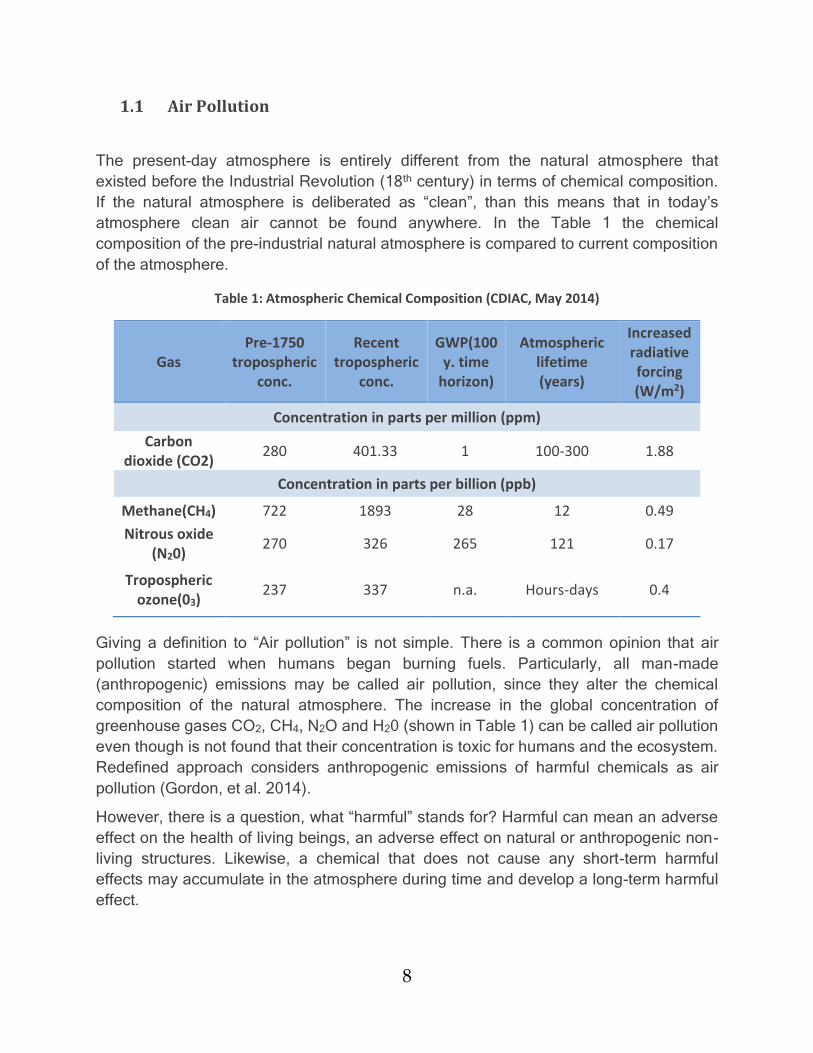
atmosphere clean air cannot be found anywhere. In the Table 1 the chemical

composition of the pre-industrial natural atmosphere is compared to current composition

of the atmosphere.

Table 1: Atmospheric Chemical Composition (CDIAC, May 2014)

Gas Pre-1750

tropospheric conc.

Recent tropospheric

conc.

GWP(100y. time

horizon)

Atmospheric lifetime (years)

Increased radiative forcing (W/m2)

Concentration in parts per million (ppm)

Carbon dioxide (CO2)

280 401.33 1 100-300 1.88

Concentration in parts per billion (ppb)

Methane(CH4) 722 1893 28 12 0.49

Nitrous oxide (N20)

270 326 265 121 0.17

Tropospheric ozone(03)

237 337 n.a. Hours-days 0.4

Giving a definition to “Air pollution” is not simple. There is a common opinion that air

pollution started when humans began burning fuels. Particularly, all man-made

(anthropogenic) emissions may be called air pollution, since they alter the chemical

composition of the natural atmosphere. The increase in the global concentration of

greenhouse gases CO2, CH4, N2O and H20 (shown in Table 1) can be called air pollution

even though is not found that their concentration is toxic for humans and the ecosystem.

Redefined approach considers anthropogenic emissions of harmful chemicals as air

pollution (Gordon, et al. 2014).

However, there is a question, what “harmful” stands for? Harmful can mean an adverse

effect on the health of living beings, an adverse effect on natural or anthropogenic non-

living structures. Likewise, a chemical that does not cause any short-term harmful

effects may accumulate in the atmosphere during time and develop a long-term harmful

effect.

9

The modern definition for the air pollution states that it represents any substance

emitted into the air from an anthropogenic, biogenic or geogenic source1, that is present

in the higher concentrations that the natural atmosphere, and may cause short-term or

long-term adverse effects (Zaneti et al., 2007).

1.2 Air Pollution Occurrences

Air pollution represents a major health risk factor across the globe. Its complexity

reflects in a fact that it cannot be easy controlled, since a lot of factors are driving it.

The most obvious factor influencing air pollution is the quantity of contaminants emitted

into the atmosphere. However, trends in air pollution are not caused by a drastic

increase in the output of pollutants; instead these trends are driven by changes in

certain atmospheric conditions.

Two of the most important atmospheric conditions affecting the dispersion of pollutants

are:

1. the strength of the wind and

2. the stability of the air

The direct effect of wind speed is to influence the concentration of pollutants. Referring

to that, global wind trends are represented on the Image 1.

Figure 1: Global Wind Trends (Global sailing weather, May 2014)

1 Geogenic emissions are produced by non-living world, e.g. natural fires, volcanic emission etc.

10

On the contrary, atmospheric stability determines the extent to which vertical motions

will mix the pollution with cleaner air above the surface layers (Pateraki et. al. 2014).

The vertical distance between Earth’s surface and the height to which convectional

movements extend is called Mixing depth. Generally, the greater the mixing depth, the

better the air quality is (Csavina et al. 2014).

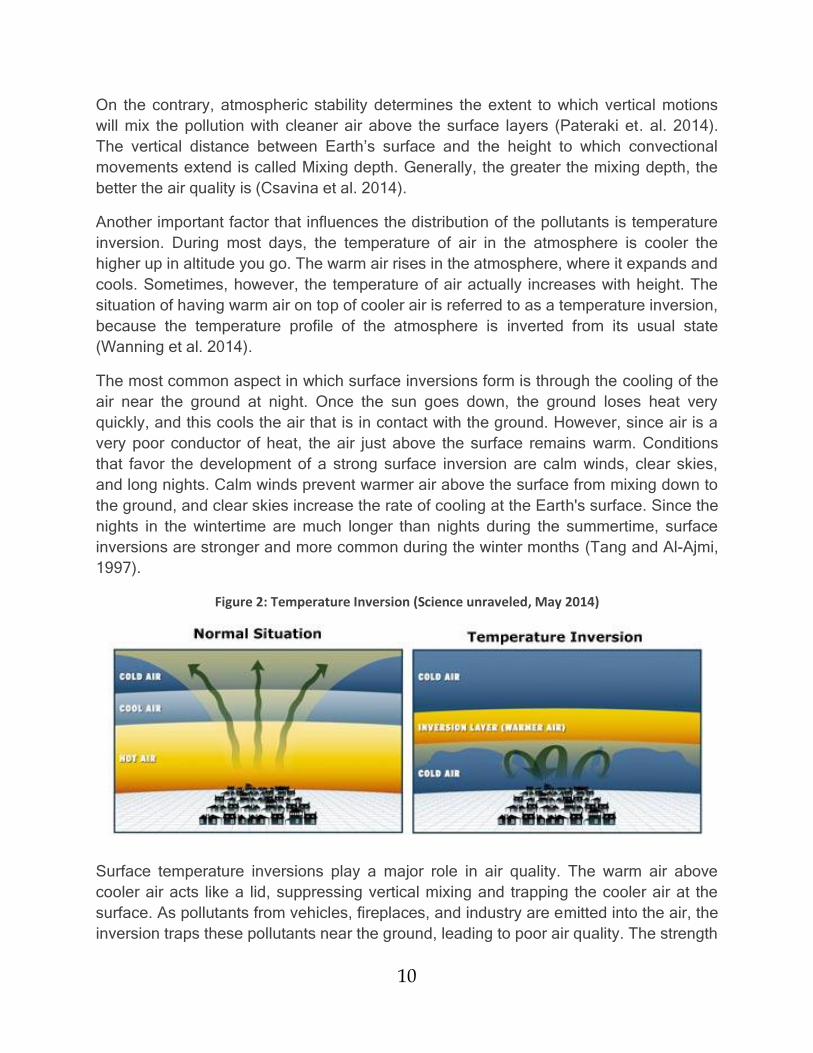
Another important factor that influences the distribution of the pollutants is temperature

inversion. During most days, the temperature of air in the atmosphere is cooler the

higher up in altitude you go. The warm air rises in the atmosphere, where it expands and

cools. Sometimes, however, the temperature of air actually increases with height. The

situation of having warm air on top of cooler air is referred to as a temperature inversion,

because the temperature profile of the atmosphere is inverted from its usual state

(Wanning et al. 2014).

The most common aspect in which surface inversions form is through the cooling of the

air near the ground at night. Once the sun goes down, the ground loses heat very

quickly, and this cools the air that is in contact with the ground. However, since air is a

very poor conductor of heat, the air just above the surface remains warm. Conditions

that favor the development of a strong surface inversion are calm winds, clear skies,

and long nights. Calm winds prevent warmer air above the surface from mixing down to

the ground, and clear skies increase the rate of cooling at the Earth's surface. Since the

nights in the wintertime are much longer than nights during the summertime, surface

inversions are stronger and more common during the winter months (Tang and Al-Ajmi,

1997).

Figure 2: Temperature Inversion (Science unraveled, May 2014)

Surface temperature inversions play a major role in air quality. The warm air above

cooler air acts like a lid, suppressing vertical mixing and trapping the cooler air at the

surface. As pollutants from vehicles, fireplaces, and industry are emitted into the air, the

inversion traps these pollutants near the ground, leading to poor air quality. The strength

11

and duration of the inversion will control air quality impact levels near the ground. Strong

inversion will confine pollutants to a shallow vertical layer, leading to high impacts on the

air quality, while a weak inversion will lead to lower impact levels. (NOAA, May 2014).

1.3 Type of Air Pollution

Air pollutants are any gas, liquid or solid substance that have been emitted into the

atmosphere and are present in a concentration high enough to be considered as

harmful to the environment, or human, animal and plant health.

Air pollutants may be either emitted directly into the atmosphere so called “primary air

pollutant” or formed within the atmosphere itself by reaction with other pollutants,

“secondary air pollutants”.

Primary air pollutants are those which are emitted directly into the atmosphere from a

source, such as factory chimney, exhaust pipe or through suspension of contaminated

dust by the wind. Considering the mechanism of their appearance, it is possible to

measure the amounts emitted at the source itself.

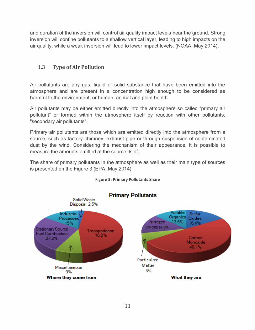
The share of primary pollutants in the atmosphere as well as their main type of sources

is presented on the Figure 3 (EPA, May 2014).

Figure 3: Primary Pollutants Share

12

The main primary pollutants that are known to cause harm in high enough

concentrations are the following:

Carbon compounds: CO, CO2, CH4 and VOCs,

Nitrogen compounds: NO, N2O and NH3,

Sulfur compounds: H2S and SO2,

Halogen compounds: chlorides, fluorides and bromides,

Particulate Matter (PM or aerosols), either in solid or liquid form,

Sources of primary pollutants are many. Natural sources of primary pollutants are

volcanoes, fire, bacteria, viruses, pollens, blowing dust, etc. and they are accentuated

by humans in recent history. However, the biggest contributions are causing sources

created by humans.

After the emission, air pollutants in the atmosphere undergo dispersion and

transportation, mainly due to meteorological conditions, chemical reactions and

photochemical reactions. Thus, secondary air pollutants are formed. Because of this

mode of formation, secondary pollutants cannot readily be included in emission

inventories, although it is possible to estimate their formation rates.

The main secondary pollutants that are known to cause harm in high enough

concentrations are the following:

NO2 and HNO3 formed from NO,

Ozone (O3) formed from photochemical reactions of nitrogen oxides and VOCs,

Sulfuric acid droplets formed from SO2 and nitric acid droplets formed from NO2

Sulfates and nitrates aerosols, formed from reactions of sulfuric acid droplets and

nitric acids droplets with NH3, respectively,

Organic aerosols formed from VOCs in gas-to-particle reactions.

Another important distinction must be made in relation to the physical state of the

pollutant. There are two categories: gas and particle. Gaseous air pollutants are those

present as gases or vapors. They are readily taken into the human respiratory system

and very often are precursors of adverse effects to human health. Gaseous air

pollutants include NO2, SO2, CO, O3, NH4, VOCs, vapor phase of semi-volatile organic

compound, etc. Particulate air pollutants mainly refer to fine particles in solid or liquid

phase suspended in the atmosphere. Such particles can be either primary or secondary

and cover a wide range of sizes.

Apart from the physical state it is also important to consider the geographical location

and distribution of sources as well as their geographical scale (point, line or area

sources). Depending primarily on the atmospheric lifetime of the specific pollutants, the

local, regional and global scale of air pollution can be distinguished (WHO, May 2014).

13

1.4 Particulate Matter

Particulate matter, also known as particulate pollution or PM represents a complex

heterogeneous mixture of liquid droplets and extremely small particles having diverse

chemical and physical characteristics. It encompasses many different chemical

components such as organic chemicals, metals, acids (such as nitrates and sulfates)

and soil or dust particles, many of which have been specified as potential contributors to

toxicity. Each of these components has multiple sources and each source generates

multiple components. Sulfur dioxides and nitrogen oxides, known as secondary particles

make up most of the fine particle pollution (Kelly and Fussell, 2012).

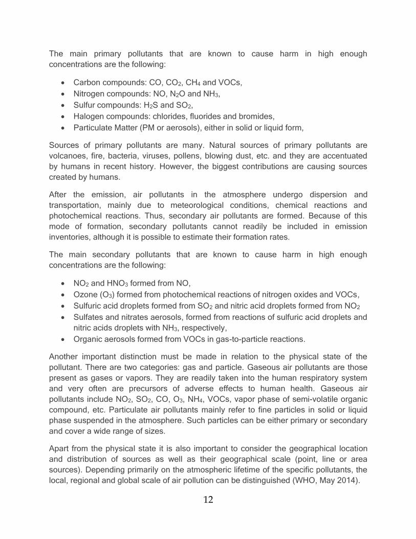
The size of particles is directly linked to their potential for causing health problems

(Figure 4). Particles can be solid particles or liquid droplets which diameters are ranged

from 0.1-50 micrometers. Those particles are called total suspended particles (TSP).

Small particles, less than 10 micrometers in diameters cause the greatest problems,

because they can get deep into lungs, and some may even reach bloodstream. Small

particles which diameters are less than 10 micrometers are further divided into two

major groups according to the size. Generally, inhalable coarse particles with diameter

smaller than 10 micrometers and larger than 2.5 micrometers (PM10) and fine particles

with diameters that are 2.5 micrometers and smaller, (PM2.5).

Figure 4: Particulate Matters Size (EPA, May 2014)

14

Inhalable coarse particles or PM10, are mainly mechanically produced by the break-up of

larger solid particles. In urban areas, the coarse particles typically contain resuspended

dust from roads and industrial activities, and biological material such as pollen grains

and bacterial fragments. Typically, these particles also include wind-blown dust from

agricultural activities, uncovered soil or mining operations. Near coasts, evaporation of

sea spray can also produce large particles. Coarse particles may also be formed from

the release of non-combustible materials in combustion processes, i.e. fly ash.

Fine particles, those smaller than 2.5 micrometers, are largely formed from gases.

However, combustion processes may also generate primary particles in this size range.

Generally, these particles originate as ultrafine particles (nuclei) produced by chemical

reactions in the atmosphere, from various processing of metals, driving automobiles or

burning plants.

Smaller particles are lighter and they stay in the air longer and travel further. PM10 stay

in the air for minutes or hours, while PM2.5 can stay in the air for days or weeks.

Regarding the travel distance, PM10 particles can travel from few hundreds of meters up

to 50km, still PM2.5 can go even further, many hundreds of kilometers (Stephanou,

2012).

The particle matters may become dangerous to our health when we are exposed to it for

a long time, and also when we breathe in a large amount of it. Apart from that, health

effects can be acute or chronic. Acute health effects are characterized by sudden and

severe exposure and rapid absorption of the substance. Normally, a single large

exposure is involved and health effects are often reversible. On the contrary, chronic

health effects are characterized by prolonged or repeated exposures over many days,

months or years. Symptoms may not be immediately apparent. These kinds of effects

are often irreversible (OSHA, May 2014).

Epidemiological studies have found a broad number of evidences on the association

between exposure to air pollution and cardiovascular events. Scientific statement on

particulate matter made by the first American Heart Association (AHA) concluded that

short-term exposure to PM contributes to acute cardiovascular morbidity and mortality.

Likewise long-term exposure may reduce life expectancy.

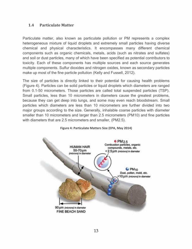
Notwithstanding, ambient air quality has been improved on the global scale in the past

decade (Figure 5.), by following current policies for its abatement. But despite regulatory

effort, fine particulate continues to be a matter of concern despite its falling trend.

Protection of human health is further deteriorated considering the inability of scientists to

establish a safe level of PM2.5 below which it poses very little or no effect on human

health. Furthermore, the effect of particulate matter on health is very complex since it

may vary from one individual to another. It must be taken into consideration that not all

individuals are equally vulnerable to air pollution health effects. Vulnerability could be

15

strictly linked to individual characteristics such as genetics, age, gender and the life

style. For instance, low socioeconomic classes tend to be more vulnerable to adverse

effects of air pollution considering their lower quality of life caused by other factors.

Hence, analysts must calculate changes in health outcomes by taking into account that

effect of pollution may be easily correlated with other elements that may be just as

influential (Nazelle et al. 2011).

Figure 5: Global Trend of PM10 and PM2.5 (EEA, May 2014)

Exposure to PM can affect both your lungs and heart. PM2.5 travels deeper into the lungs

and since it is made of components which are more toxic (heavy metals), PM2.5 can

have worse health effects than the bigger PM10. Numerous scientific studies have

associated particle pollution exposure to a variety of problems, including:

Irregular heartbeat,

Aggravated Asthma

Lung damage (including decreased lung function and lifelong respiratory disease)

Nonfatal heart attacks,

Premature death with people with heart or lung disease

Increased respiratory symptoms, such as irritation of the airways, coughing or

shortness of breath (Koton et al. 2013).

16

On the other hand, epidemiological studies have shown that pollution acts

synergistically with tobacco smoking, alcohol consumption and unhealthy diet to induce

respiratory illness such as asthma, lung cancer and cardiovascular diseases.

However, there is a general agreement among scientists that fine particle matter (PM2.5)

composition also plays a meaningful role in the health effects attributed to PM.

Composition of PM may be more substantial than PM concentration alone in explaining

health impacts. As evidence linking composition to health impacts emerges in the

epidemiological and toxicological areas, it is becoming more urgent to distinguish which

components or combination of components are the most harmful to human health.

Toxicological studies suggest that several elements, including aluminum, silicon,

vanadium, carbon-containing components and nickel are the most closely correlated to

health impacts. However, many other elements have been implicated as well. There are

no PM components for which there is unequivocal evidence of zero health impact (Rohr

and Wyzga, 2012).

Carbonaceous classes, elemental (EC) and organic carbon (OC) are well known

contributors to the atmospheric particulate matter at a global level, and also very

frequently dominant contributors to the fine particulate matter mass. EC is derived from

incomplete combustion of carbon-based materials and fuels and is present in primary

form in the nature, while on the other hand OC may be directly released into the

atmosphere or produced by way of secondary gas-to-particle conversion process. Along

with the adverse health effects which are correlated with fine particulate matter mass

exposure, carbonaceous species inflict very serious health effects. Considering the fact

that EC is mainly considered as inert and that combustion process is deriving EC,

coated by organic matters as PAHs, which are widely known to have carcinogenic and

mutagenic properties and to cause serious health risks (Lonati et al. 2007).

Knowledge about carbonaceous portions in fine particulate matters and especially their

portioning between primary and secondary origin may be used very efficiently in

conveying new air quality plans and targets (Lonati et al. 2007).

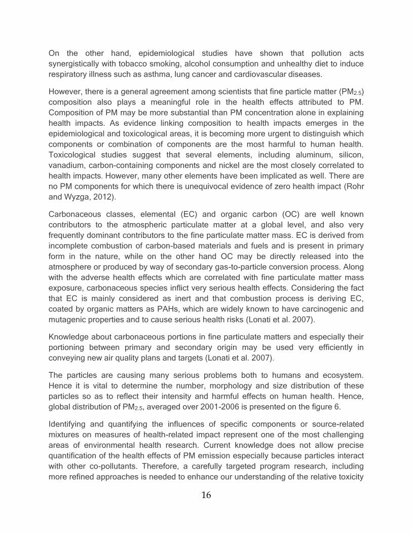
The particles are causing many serious problems both to humans and ecosystem.

Hence it is vital to determine the number, morphology and size distribution of these

particles so as to reflect their intensity and harmful effects on human health. Hence,

global distribution of PM2.5, averaged over 2001-2006 is presented on the figure 6.

Identifying and quantifying the influences of specific components or source-related

mixtures on measures of health-related impact represent one of the most challenging

areas of environmental health research. Current knowledge does not allow precise

quantification of the health effects of PM emission especially because particles interact

with other co-pollutants. Therefore, a carefully targeted program research, including

more refined approaches is needed to enhance our understanding of the relative toxicity

17

of particles. This approach will facilitate development of abatement policies, more

effective pollution control measures and a reduction in the rate of health problems

caused by particulate pollution.

Figure 6: Global Satellite Deriver Map of PM2.5, averaged over 2001-2006 (WUWT, May 2014)

Besides health problems to humans, particulate pollution also drives other damages.

For instance, fine particles PM2.5 are the main cause of reduced visibility (haze). In a

form of acid rain they can damage stone and other materials, including culturally

important statues and monuments. Acid rain refers to a mixture of wet and dry

deposition from the atmosphere containing higher than normal amounts of nitric and

sulfide acids. It can appear in a form of rain, snow, fog and tiny bits of dry material that

settle on Earth. Origin of formation of such rains lies in the PM either from natural

sources or from anthropogenic sources. Considering the fact that particles can be

carried over a long distances by wind and then settled on ground or water, this effect

can make also lakes and streams acidic. By settling into the other mediums, particles

may also change theirs nutrient balance, damage sensitive forests and farm crops,

deplete nutrients in soil and lastly affect the diversity of ecosystem (Liang, 2013).

Apportionment of pollution sources should be the main interest in development of

current strategies and regulations of the environment. It is important to acquire as many

information as possible about the sources of pollution we are exposed to, as well as

characteristics and concentration of those sources. Hence, if a specific source that

contributes to air pollution in a given area is known, than strategies can be planned and

implemented in a way that reduces the impact of those sources. Additionally, by

knowing the type of the sources that are contributing the most to the air pollution,

18

awareness of the people may be raised to a higher level, thus they can make some

modifications in their life style and habits.

1.5 Trends and Projections

Europe needs more resource efficient, greener and competitive economy. Consumers

who appreciate resource efficiency, new green technology and smart inventions toward

sustainability can create new economic opportunities. By developing cleaner and more

efficient energy, this green industry can create new jobs and this approach can as well

reduce Europe’s import of oil and gas and improve its position on the energy market.

With development of such technologies, it will not be achieved just improvement

towards the environmental sustainability but at the same time and economic recovery

(ESPON, May 2014).

Accordingly, some of the main trends present nowadays are as follows:

Waste treatment processes in EU have improved remarkably since 2000.

Landfilling represents one of least environmental-friendly technics for managing

waste. Accordingly incinerators started gradually replacing them with a greater

frequency by applying composting and recycling techniques. About 40% of

municipal waste was recycled or composted. However, there are huge

fluctuations in techniques used in some countries in Europe. For instance, in

Bulgaria, Croatia and Romania more than 90% of waste was landfilled, where on

contrary in Germany, the Netherlands and Sweden this approach was below 1%.

Current estimates are showing that the extent of the effects of ozone and fine

particle pollutants on life expectancy is in the order of several tens to hundreds of

thousands of premature deaths per year in Europe (WHO, 2006). Despite the fact

emissions of air pollutants are generally declining, many countries are not jet on a

track towards EU targets and air quality limit values for PM10, PM2.5 and NO2.

Even if the emission reduction targets are met, health impacts are still likely to

occur. However, this appears partly due to background levels and natural

sources of these compounds, which is impossible to address from a European

perspective only.

Energy consumption in Europe peaked in 2005 and has been declining since.

This trend decelerated slightly until 2010, partly due to the economic crisis and

limited economic recovery in 2010. This result is clearly due to implementation of

energy efficiency and renewable energy policies, where the economic crisis and

structural changes also played a significant role in the most recent trends taking

also into account milder winters. More recently, primary energy consumption in

Europe was 14.4 higher than the 2020’s set target. The most significant decrease

19

occurred in Germany, France, Spain, Italy and the United Kingdom. The

economic crisis was more pronounced in these countries especially in the

industry and transport sectors. Also, the switch of fuels played a major role in this

decrement. Lastly, in 2011, the final energy consumption in EU-28 was only 2.4%

higher than the 2020’s set target.

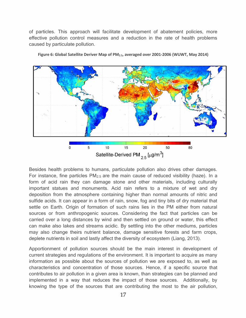
On the other hand, there is a rapid expansion on renewable energies, particularly

in electricity sector (Table 2). Energy generated from biomass, wind, solar energy

and the Earth’s heat are replacing share of fossil fuels in the final energy demand

in the EU. Between 2005 and 2011 all member states of the EU have increased

their renewable energy share. While it is asserted the greatest expansion in wind

and solar energy, however contribution of biomass represents by far the largest

amount. In conclusion, renewable energy sources are covering a fifth of gross

power generation in 2011.

Despite the fact the gap in CO2 emissions per capita narrowed between the EU

and developing countries from 2000 to 2011, the CO2 emissions remained at 7.4

tones per capita in the EU, which is 2.6 times greater than the developing country

average of 2.9 tones per capita. This narrowing of gap occurred primarily as a

result of increasing emissions from developing countries and on the other hand

financial crisis which led to reduction of CO2 emissions per capita in the EU

(Eurostat, May 2014).

Table 2: Contribution by Renewable Energy Carriers (electricity, heating/cooling, transport) (EEA, May

2014)

Energy (Mtoe) Share (%)

Year 2005 2010 2011 2020 2020

RES-E 41.4 55.9 60.7 104.2 42

RES-H/C 58.9 78.4 76.7 111.5 46

RES-T(including biofuels)

1.0 (4.2)

10.5 (14.4)

11.5 (15.0)

29.5 12

Total RES (including biofuels)

100.3 (103.4)

143.6 (147.6)

147.2 (151.2)

245.1 100

Current estimates are indicating that EU is having 7.7% of the world’s population and

contains 9.5% of the world’s biocapacity. Ability of the system to generate biological

materials and to absorb waste materials produced by humans accounting current

management approaches and technologies is called biocapacity. Despite having above

average biocapacity with respect to its population, EU generates 16% of the world’s

ecological footprint. What is more, EU’ development strongly depends on the ecological

reserves in other parts of the world.

20

Nevertheless, some scientists believe that large-scale biomass plants could accelerate

deforestation or endanger local biodiversity. These observations are not an argument

against evolution of biomass as a new renewable energy industry. Rather they want to

emphasize the need for an integrated approach to territorial development.

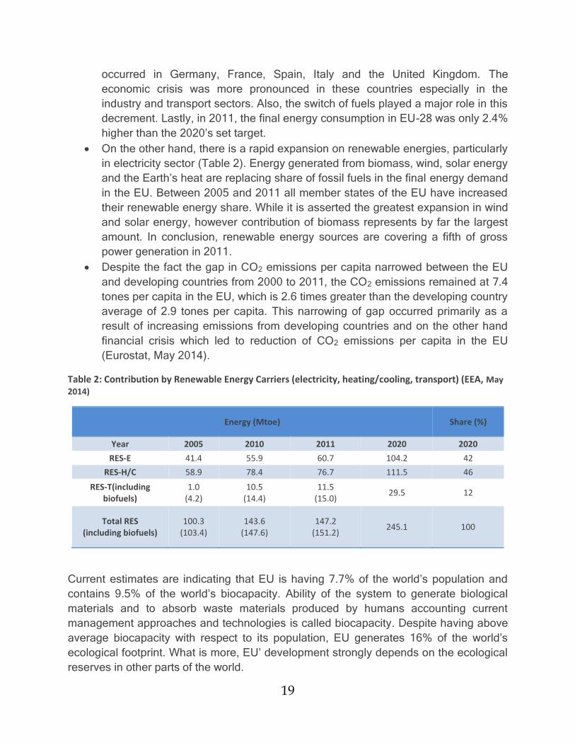
Considering other renewable sources of energy, mainly solar and wind, it can be said

that great expansion is currently being made and still there is a lot of potential in these

fields. The map of Europe with yearly total yield of estimated solar electricity generation

(kWh) and production potential of wind power stations, taking into account

environmental and other constraints are presented on figure 7 and figure 8. From the

maps it can be seen that the North Europe dominates in a potential for wind production,

while Southern Mediterranean Europe dominates in the high potential for a generation of

energy using Sun energy.

The EU-15 has a common objective to be achieved collectively under the Kyoto

Protocol. This protocol in an international agreement linked to the United Nations

Framework Convention on Climate Change, which sets binding obligations on countries

to reduce emissions of greenhouse gasses. It sets emission limitations and reduction

targets for each EU-15 Member State. Each of the targets corresponds to an emission

budget (“Kyoto units”) for the first commitment period (2008-2012) of the Kyoto Protocol.

Nearly all Member States and all other European Environment Agency (EEA) countries

achieved targets set by Kyoto protocol by the end of the Kyoto Protocol’s first

Figure 7 and 8: Yearly Total Yield of Estimated Solar Electricity Generation (kWh) and Production Potential of Wind Power Stations. (ESPON, May 2014)

21

commitment period, i.e. the target was set to 8% of reduction for the period of 2008-

2012 compared to base-year levels under the Kyoto Protocol and EU-15 have reached

reduction of 12.2%.

However, as in previous years, Italy remains considered off track towards the target,

mainly due to lack of information on its planned use of flexible mechanisms. Italy did not

put a threshold on the use of flexible mechanisms in its national climate change

strategy, but administrative arrangements are being taken for purchases (EEA, 2013).

Europe 2020 calls for a perception of structural and technological changes in order to

move to low carbon, resource efficient and climate resilient economy by 2050. This

progression will enable Europe to meets its emission reduction targets. It will include

new business growth to sustain Europe’s leading role in green technologies on the

international market, but also disease prevention and response as well as adjustment

measures based on more efficient use of resources.

The EU has set 5 targets to be reached until 2020. These targets are mainly focused on

improvement of employment rates, greenhouse gases reduction, poverty reduction and

enhancement of educational attainment and health. Likewise, “20/20/20” represents the

triple objective for 2020. There targets are endorsed by the European Council in 2007

and implemented through the EU’s 2009 climate and energy package and the 2012

Energy Efficient Directive, and it focuses on:

A 20% increase in energy efficiency

A reduction in greenhouse gas emissions by at least 20% compared to 1990

levels.

To develop renewable energy resources so that they can account for 20% of total

energy consumption (ESPON, May 2014).

The time scale is fundamental to implementing methods for a higher sustainability.

Europe 2020 represents a short-term time horizon with respect to economic

development and short-term horizon from the perspective of Europe’s sustainable

development. Accordingly, it is very important to look further into the future and not just

into the meeting the current targets. This is fundamental as environmental impacts are

long lasting, climate change is a long-term process and patterns of urban areas, energy

and transport networks need time to adapt.

The territorial impacts on the scenario are under change over time. The primary impact

is caused by the metropolitan regions, mainly in Western Europe, thus the greatest

expectations in investments in new technologies are expected to be made in this region.

However, in the later phase of the scenario there is a diffusion of these ideas and a

more polycentric pattern of growth. Nonetheless, it is important to identify that such

22

approach carries more challenges for some regions than for others. South and East

European cities might be more confronted by sustainable issues, as they have less

advanced public transport systems, more polluting cars, buses and trucks, lower amount

of green areas, old technology etc.

1.6 Need for Source Apportionment

Abatement of pollution at its source represents one of the main principles of the

Thematic Strategy on Air Pollution. Information on pollutant sources is essential to the

design of air quality policies. Therefore, source apportionment is required for the

implementation of the Air Quality Directives (Dir.2008/50/EC and Dir.2004/107/EC). For

instance, the true pollution source information is required in order to identify whether

possible overcoming are due to natural sources or to artificial ones, set the limit values

of pollutants, preparing air quality plans, quantifying trans-boundary pollution, and

informing the public (Belis et al., 2014).

Particulate matter (PM) is one of the main pollutants exceeding the ambient standards

for air quality in Europe. Majority of suspended particles are too small to be seen with a

human vision. Even if they are identified with some magnification technique, their origin

very often remains unknown. A variety of sources contribute to a specific event and the

proportions of these contributions change from event to event, driven by many

influencers. Some particles preserve the forms in which they were originally emitted, but

others are created from emitted gases through chemical reactions, or they undergo

chemical transformations that change their chemical and physical characteristics. These

facts has let to numerous studies focusing upon its complex composition, toxicology and

source attribution (Watson and Chow, 2007).

One of the most powerful tools for the formulation of abatement policies and verification

of their effectiveness is particulate matter source apportionment by the combination of

chemical and statistical analysis. Source apportionment is the practice of deriving

information about pollution sources and the amount they contribute to ambient air

pollution levels (Frao et al. 2013).

Different approaches are used to determine and quantify the impacts of air pollution

sources on air quality. Commonly used techniques are:

Explorative methods

Emission inventories

Inverse modelling

23

Artificial neural networks

Lagrangian models

Gaussian models

Eulerian models

Receptor models

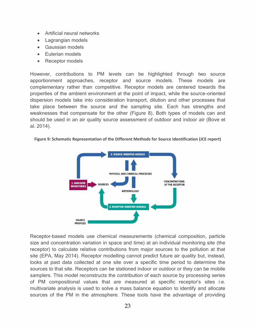
However, contributions to PM levels can be highlighted through two source

apportionment approaches, receptor and source models. These models are

complementary rather than competitive. Receptor models are centered towards the

properties of the ambient environment at the point of impact, while the source-oriented

dispersion models take into consideration transport, dilution and other processes that

take place between the source and the sampling site. Each has strengths and

weaknesses that compensate for the other (Figure 8). Both types of models can and

should be used in an air quality source assessment of outdoor and indoor air (Bove et

al. 2014).

Figure 9: Schematic Representation of the Different Methods for Source Identification (JCE report)

Receptor-based models use chemical measurements (chemical composition, particle

size and concentration variation in space and time) at an individual monitoring site (the

receptor) to calculate relative contributions from major sources to the pollution at that

site (EPA, May 2014). Receptor modelling cannot predict future air quality but, instead,

looks at past data collected at one site over a specific time period to determine the

sources to that site. Receptors can be stationed indoor or outdoor or they can be mobile

samplers. This model reconstructs the contribution of each source by processing series

of PM compositional values that are measured at specific receptor’s sites i.e.

multivariate analysis is used to solve a mass balance equation to identify and allocate

sources of the PM in the atmosphere. These tools have the advantage of providing

24

information derived from real-world measurements, including estimations of output

uncertainty. However, these models can be unsuccessful with reactive species and may

perform better in areas relatively closer to the sources (Bove et al. 2014).

Receptor models have been widely used over past three decades to apportion ambient

concentrations to sources. Among these, the Chemical Mass Balance (CMB), Principal

Component Analysis (PCA) and Positive Matrix Factorization (PMF) methods are the

most frequently used. CMB can be used if sources and emission profiles of PM are

known “a priori”. However, a detailed knowledge of sources and emissions is not always

available; in these cases it is preferable to use multivariate models like PCA and PMF,

which attempt to apportion the sources on the basis of the internal correlations at the

receptor site.

The main output from these models is an estimate of the contributions from each source

to the air pollution at that site. However, the reliability of receptor model outputs

depends on appropriate data collection, in terms of data capture and kind of chemical

species, and proper expression of uncertainty in the input data. This represents an

aspect particularly relevant in PMF, which scales data on the basis of their uncertainty.

In addition, determining the number of relevant sources and establishing the

correspondence between factors and sources still appear as critical steps. Results from

these models are important for scientifically justifying priorities and observing trends.

Moreover, this scientific information helps air quality modelers as well as policy and

decision makers (EC, June 2014).

An alternative to the statistical data analyses is given by simpler models based purely

on chemical analysis of dominant PM components and is called source models. Source

models estimate concentrations at receptor coming from different source emissions and

being influenced by meteorological measurements. Basically, chemical determinations

are individually summed up in order to obtain a mass closure and then grouped to

determine the macro-sources of PM. To enhance the selectivity of the elements as

source tracers, a size fractionation of PM can be performed, as it is well known that fine

particles (< 2.5 μm) are mainly emitted from combustion sources and coarse particles (>

2.5 μm) are generated from mechanical-abrasive processes (Watson et al., 2002).

Within the activities of the Forum for Air Quality Modelling in Europe (FAIRMODE) group

on “Contribution of natural sources and source apportionment”, few surveys were

implemented with the focus on the type and frequency of model used for source

apportionment in Europe. When examining the received information on the most recent

survey (Fragkou et al. 2012) it becomes obvious that the different tools for source

identification in Europe ranged from less than 20% for Gaussian models to almost 60%

for receptor models used in Europe (Figure 9). Furthermore, among all technologies

25

used in Europe, the most used models in Italy are Receptor (CMB, PMF2, PMF3) and

Dispersion-Eulerian (FARM, CAMx/PSAT) models.

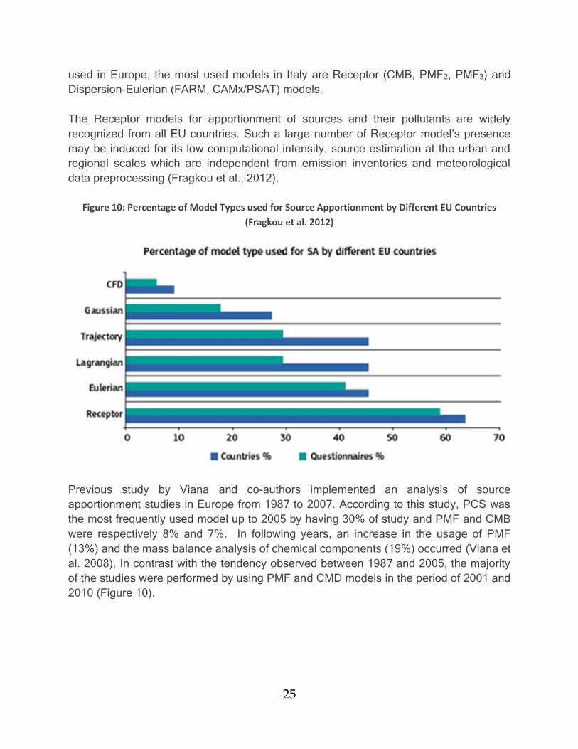
The Receptor models for apportionment of sources and their pollutants are widely

recognized from all EU countries. Such a large number of Receptor model’s presence

may be induced for its low computational intensity, source estimation at the urban and

regional scales which are independent from emission inventories and meteorological

data preprocessing (Fragkou et al., 2012).

Figure 10: Percentage of Model Types used for Source Apportionment by Different EU Countries

(Fragkou et al. 2012)

Previous study by Viana and co-authors implemented an analysis of source

apportionment studies in Europe from 1987 to 2007. According to this study, PCS was

the most frequently used model up to 2005 by having 30% of study and PMF and CMB

were respectively 8% and 7%. In following years, an increase in the usage of PMF

(13%) and the mass balance analysis of chemical components (19%) occurred (Viana et

al. 2008). In contrast with the tendency observed between 1987 and 2005, the majority

of the studies were performed by using PMF and CMD models in the period of 2001 and

2010 (Figure 10).

26

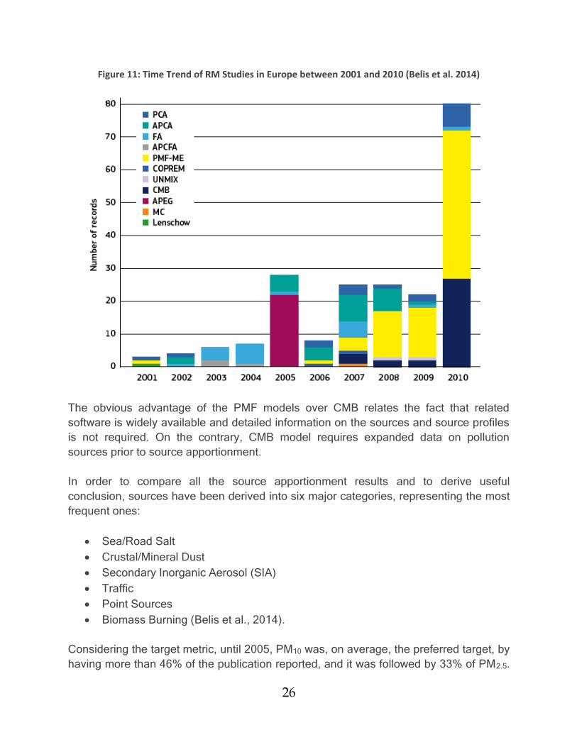
Figure 11: Time Trend of RM Studies in Europe between 2001 and 2010 (Belis et al. 2014)

The obvious advantage of the PMF models over CMB relates the fact that related

software is widely available and detailed information on the sources and source profiles

is not required. On the contrary, CMB model requires expanded data on pollution

sources prior to source apportionment.

In order to compare all the source apportionment results and to derive useful

conclusion, sources have been derived into six major categories, representing the most

frequent ones:

Sea/Road Salt

Crustal/Mineral Dust

Secondary Inorganic Aerosol (SIA)

Traffic

Point Sources

Biomass Burning (Belis et al., 2014).

Considering the target metric, until 2005, PM10 was, on average, the preferred target, by

having more than 46% of the publication reported, and it was followed by 33% of PM2.5.

27

While other smaller size fractions PM2, PM1, PM0.1 had smaller share. However, different

trend occurred starting from 2006, when PM2.5 took over the lead in the share by having

38% of the new studies and on contrary only 29% focused on PM10. Thus, this new

trend shows a change of focus in source apportionment studies in Europe. This new

order may be due to the stronger recent evidences on the adverse effects of fine

particles on health with comparison to coarser particles (Viana et al. 2008).

The majority of the studies were implemented in urban areas (53% of the studies) while

industrial or kerbside sites represented respectively 11% and 20% of the studies (Viana

et al. 2008).

The results of all surveys demonstrate the simultaneous use of different modelling tools

and methods for identification and attribution of sources at investigated receptor sites,

as the applicable methodology in order to combine the advantages and reduce the

constrains of the individual model components. Moreover, the trends in usage are

changing rapidly due to new discoveries on adverse effects of particulate matter mainly

on the human health.

1.7 Scope of the Work

The fundamental objective of this work is to give contribution to better understanding of

the nature of PM and to quantify relative significance of diverse emission sources and

enable decision makers to convey efficient air quality remediation plans. Thus, the

scope of this work is to perform a PM source apportionment by means of the PMF

model on the PM data set from Milan2.

In the recent past years during PM monitoring campaigns the data set is acquired with

an aim to define the composition and contributions of various species to PM2.5 bulk mass

in Milan. Thus, this work will contribute to enrichment of the current records for the

specified area.

The main focus is on PM2.5, since recent air quality standards for PM inquired by

European Union, studies also PM2.5, besides PM10, where were specified both,

concentration limits and an exposure reduction target. The second reason for

centralizing on PM2.5 is that anthropogenic carbon forms are almost completely included

in fine PM (Lonati et al., 2007).

2 The city of Milan is situated in the Lombardy region and is surrounded by many industrial zones;

Furthermore, the metropolitan area of the city has a population of over 4 million people.

28

2 Model Application and Material

2.1 PMF Application

PMF represent a recent development in the data analysis technique’s sphere, which is

called factor analysis. The main problem in these techniques is to resolve the identity

and contribution of components in an unknown mixture. PMF is particularly applicable in

the projects that use environmental data, for the following reasons:

1. It integrates the uncertainties of variables which are often associated with

measurements of environmental samples

2. It drives all the values in a solution profiles and contributions to be non-negative,

which represents more realistic approach than previously used models

PMF is being used to categorize and apportion sources of airborne PM, by collecting

data in numerous locations in the World. Mainly the collection locations are being

focused in the urban areas, since there is the biggest need for the knowledge of the

ambient air components. Likewise, classification of PM is set as PM<1µm (PM1),

<1PM<2.5 µm (PM2.5) and PM<10 µm (PM10). This information is used for

categorization of the PMF case studies with respect to PM.

These data sets are principally used to identify profiles and contributions of PM from

primary sources; for instance, motor vehicles, residential and industrial fuel

consumption, biomass burning, soil dust and sea salt. Likewise, secondary sources,

such as atmospheric oxidation of sulfate and nitrate and heterogeneous gas-to-particle

conversion reactions on soil dust surfaces, are as well subject to the PMF application.

(Prakash V. Bhave, et. al. 2007)

After consideration of the primary use of PMF, there are many more fields of application

for this model, and many new ones are being under feasibility study.

Chemical composition of soil samples are multivariate in nature and hence represent the

ideal data for the multivariate factor analytical techniques (PMF) and for its

approximation. Recent enhancements of the model led to the increased application

within this field of study. The reason lies in the fact that previous approaches used for

the analysis of soil datasets, did not rely strongly on physically significant assumptions.

By combining results from PMD model with geostatical approach, it was possible to

successfully determine the main sources of the combined organic and heavy metal

contamination. (S. Vaccaro et.al. 2007)

Another combination of PMF with other approaches is used. Quantification of the diesel-

and gasoline-powered motor vehicle emissions can be identified by merging results

29

from PMF receptor modelling and on-road measurements captured by a mobile

laboratory. By obtaining firstly source profiles from the PMF, the calculation of fuel-

based emission factors for each type of the exhaust is possible. (D.A. Thornhill, et.al.

2010)

On the other hand, PMF application within the research and development facility

emissions is very convenient. The processes are varying and because of that the nature

of research and number of chemicals are being changed rapidly, and PMF was the ideal

match since it was able to identify the biggest number of source-related factors, while

other approaches did not achieve such a good results. PMF is able to accept the

boundaries with little reduction in model fit. (M. Y. Ballinger and T.V. Larson, 2014)

Eco-efficiency indicators are very significant tool if researchers want to create physically

meaningful information to policy makers. PMF is limiting its results to be non-negative,

and with it two important advantages over traditional factor analysis are achieved.

Firstly, the rotational ambiguity of the solution space is reduced. Secondly, all the results

are guaranteed to be physically meaningful. (J. Wu et.al. 2012)

PMF, however, finds its place in a very technical area of studies as well. Time-resolved

optical waveguide absorption spectroscopy (OWAS) is a technique used for the

investigation of kinetics at the solid/liquid interface of dyes, pigments, fluorescent

molecules, quantum dots, metallic nanoparticles, and proteins with chromophores. The

application of PMF to these techniques is quite recent, but it is already proved that it

prevents the negative factors from occurring, avoids contradicting physical reality and

makes factors more easily interpretable. (P. Liu et.al. 2013)

On the contrary of PMF extensive use, there are significant fluctuations in the procedure

process for the source apportionment. This procedure may be separated into three

broad steps:

1. Preparation of data to be modeled

2. Processing the data with PMF with an aim to develop a realistic and robust

solution

3. Interpretation of the solution

Some specific decision making are needed in the above mentioned steps, towards the

choice of data uncertainties’ set, selection of factors and treatment of outliers.

30

2.2 PMF within Europe

Danube River represents the second longest river in the Europe. Its spring starts in the

Germany’s Black forest and it flows until its delta on the Black Sea. Considering its size

and impact that generates, the chemical composition of the river and its tributaries

should be well identifiable. In the past, some monitoring programs were performed in

various parts of its drainage basin, taking into consideration its tributaries as well, with

an aim to quantify the micro-pollutants level in the river. However, as new methods were

developed, PMF was used with an objective to identify both natural and anthropogenic

sources affecting Danube basin, as well as origin of heavy metals and other possible

sources affecting the sediment creation. With applied PMF method, the spatial

distribution of resulting sources was used to identify the role of the tributaries as

potential sources of pollution. Results showed that the majority of tributaries are

influenced by the anthropogenic sources. For instance, Velika Morava River has very

high concentration of metal in sediments which can be influenced by the mining activity

in the catchment area. On the other hand, the Sava tributary showed elevated values of

mercury, probably in association with old refinery activities and chemical industry. In

conclusion, the PMF application identified one anthropogenic parameter, which could be

linked to different anthropogenic activities depending on the location along the Danube

River: municipal and industrial discharge and mining activity (S.Comero et. Al. 2014).

One of the hotspot areas in Europe with high concentration of particulate matter which is

having a lot of problems in meeting all standards for current legislation of PM2.5 is the

Netherlands. For the sake of better understanding of current levels, composition and

distribution and origin of PM2.5 in the ambient air, one-year measurement campaign was

run in the five locations in the Netherlands area. PMF was used as the main tool to

understand and categorize the most relevant source contributions and their spatial

variability in PM2.5. Wind direction was as well incorporated into the study of the results

from PMF with an aim to identify more accurately the possible locations of the identified

sources. (D. Mooibroek et.al. 2011)

To have a wide outlook of PM13

mass concentration and chemical composition of sub-

micron sized aerosols, two measurement campaigns were performed in three towns in

Italy, Milan, Genoa and Florence. Every town was having different characteristics with

respect to their orography, extension, population and emission sources. This campaign

represents first large-scale investigation on PM1 in Italy and likely in Europe. The aim of

this research campaign was to identify major sources of PM1, and to estimate their

contribution to mass concentration. After running the PMF model on the collected data

sets, it is identified that during the wintertime, the highest concentrations of PM1 were in

3 PM1, particulate matter with aerodynamic diameter smaller than 1 μm,

31

Milan, due to the high loading of pollutants and the atmospheric stability. Since, Po

valley where Milan is situated, has peculiar meteorological conditions and very heavy

emissions of pollutants from many different sources, it represents the most critical area

in Europe with respect to limit values exceedances. However, during summer time PM1

concentration significantly decreased in Milan. As the reason of this reduction, slower

average wind speeds and mixing layer heights were crucial influencers. On the contrary,

other two cities were showing completely different results since conditions in those

areas differ significantly with respect one in Milan area. Lastly source identification was

carried out with the help of available literature source profiles for PM1 fine fractions, by

looking at source contribution time series and by taking into consideration explained

variation values. (R. Vecchi et. al. 2008).

Data set collected in the urban area around Elche in southern Spain starting from

December 2004 until November 2005 was analyzed with PMF in order to estimate

sources profiles and their mass contributions. After running the model, six sources were

identified. However, very important it to mention that with the PMF it was possible to

distinguish Saharan dust sources from local dust sources, and to quantitatively estimate

the contributions of these two sources. (J.Nicolás et.al.2008).

Another sampling was used as well in Spain, Zaragoza city, but this time the collection

was oriented towards the PM2.5 PAH4 substances. The aim of this project was to identify

and quantify potential PAH pollution sources. As the origin of the PAH is in the fossil

fuels, it does not surprise the fact that the most influencing sources were found in coal

combustion, vehicular emissions, stationary emissions and unburned/evaporative

emissions. In an evaluation of the results of the PMF model run, some different patterns

were identified and same were studied for the identification of the potential negative

impact on the human health. Above all, lifetime cancer risk exceedances were examined

for both, warm and cold seasons. (M. S. Callén, A. Iturmendi, J.M. López, 2014)

The similar study was performed in UK National Network between 2002 and 2006. The

goal of the study was apportionment of PAH sources as well, since they are currently

generating a great deal of interest, mainly because of their high toxicity and

carcinogenicity. The project was incorporating 14 urban sites which were known for the

vast impact towards the creation of PAHs. (E. Jang, et. al. 2013).

After considering all above mentioned case studies, it can be concluded that PMF is

widely used within Europe and for many different purposes. For instance, in the first

project, PMF identified in a very complex system, major influencing sources to the

4 PAH – Polycyclic aromatic hydrocarbons are organic compounds containing only carbon and hydrogen that are composed of multiple aromatic rings. PAHs are found in fossil fuels when an incomplete combustion occurs because of insufficient oxygen. Critically, PAHs have been identified as carcinogenic and mutagenic and are considered as pollutants of concern for the potential adverse health impacts.

32

Danube River sediments. In another project conveyed in the Netherlands, the PM2.5

was examined with PMF, and relevant source contributions and their spatial variability

were categorized. PM2.5 was under study of PMF but this time direction was toward

identification of the PAH pollution sources. The studies were performed both in Spain

and UK. Taking into account particulate matters, another project was conveyed,

however this time PM1 was studied, and the project took place in Italy. Another use of

PMF was to differentiate types of sand in the Spanish south regions, thus PM10.

Accordingly, it may be concluded that PMF represents very popular method for the

identification of many different types of PMs in the vast range of European territories,

and the trend of its use is in increasing phase.

2.3 PMF Model

Receptor models represent mathematical methods for quantifying and qualifying the

contribution of sources to observed samples, based on the structure or fingerprints of

the sources. The structure of the source is identified by using analytical approaches for

the media and fundamental species or consolidation of species is needed to separate

influences. A composition data set can be shown as a data matrix X of i by j dimensions,

in which i is the number of samples and j represents number of chemical species that

were measured, with uncertainties u. The aim of the receptor model is to resolve

chemical mass balance (CMB) between measured source profiles and species

concentration. The sources profiles are described with number of factors p, the species

profile f of each source, and the amount of mass g which is created by influence of each

factor to each individual sample. The CMB equation can be resolved with many models

including 3 models that EPA has developed. In this work, EPA Positive Matrix

Factorization will be used.

PMF represents a multivariate factor analysis program that decomposes a matrix of

identified data set into two matrices, factor contributions (G) and factor profiles (F).

These factor profiles needs to be studied by the user in order to allocate the source

types that may be influencing to the same cluster, by using quantified source profile

information and emissions of discharge registers.

Results are created using the boundary condition that no sample can have significantly

negative source influence. PMD combines both user-identified uncertainties correlated

to the sample data to weight individual points and sample concentration. This

characteristic permits analyst to include confidence in the measurement process.

PMF model obliges several repetitions of the fundamental Multi-linear Engine (ME) with

an aim to categorize the most optimal factor contributions and profiles. ME is created to

33

resolve the PMF problem by aggregating two steps. Firstly, the analyst creates a table

which specifies the PMF model. Thereafter, a programmed secondary model reads the

previously created parameter table and computes the solution. The best practice is to

iterate the model approximately 20 times for the development of a solution and 100

times for the creation of the final solution, however different starting point should be

used every time.

Variability due to chemical transformation or method fluctuations can influence

considerably by causing significant differences in factor profiles among PMF runs. The

analyst needs to identify all the error estimates in PMF to comprehend the strength of

the model outcomes.

Lastly, PMF needs a data set containing a number of parameters which are measured

across various samples. Usually, PMF is used on diverse PM2.5 data sets containing

from 10 to 20 species over 100 samples. An uncertainty value that is assigned to each

specie and sample should be estimated by using the additional uncertainty data set.

This data set is designed using propagated uncertainties or other available information

such as collocated sampling precision. (EPA Positive Matrix Factorization (PMF) 5.0.

Fundamentals and User Guide)

2.3.1. Comparison to PMF 3.0

The PMF Model Development Quality Assurance Project Plan has been created to

collect comments and suggestions from users. After completion of the project, very

useful comment were used to improve the problematic features in PMF 3.0 and to

create new tools for the improvement of the results’ accuracy and error estimation; thus

to develop version 5.0.

The main difference between PMF 5.0 and PMF 3.0 is in added two key tools. Firstly,

two additional error estimation methods and secondly, source contribution and profile

boundaries are added in the newest 5.0 version. Likewise, many other features have

been added as well to enhance the software’s friendly use, e.g. ability to read in multiple

site data, etc (EPA Positive Matrix Factorization 5.0. Fundamentals and User Guide).

34

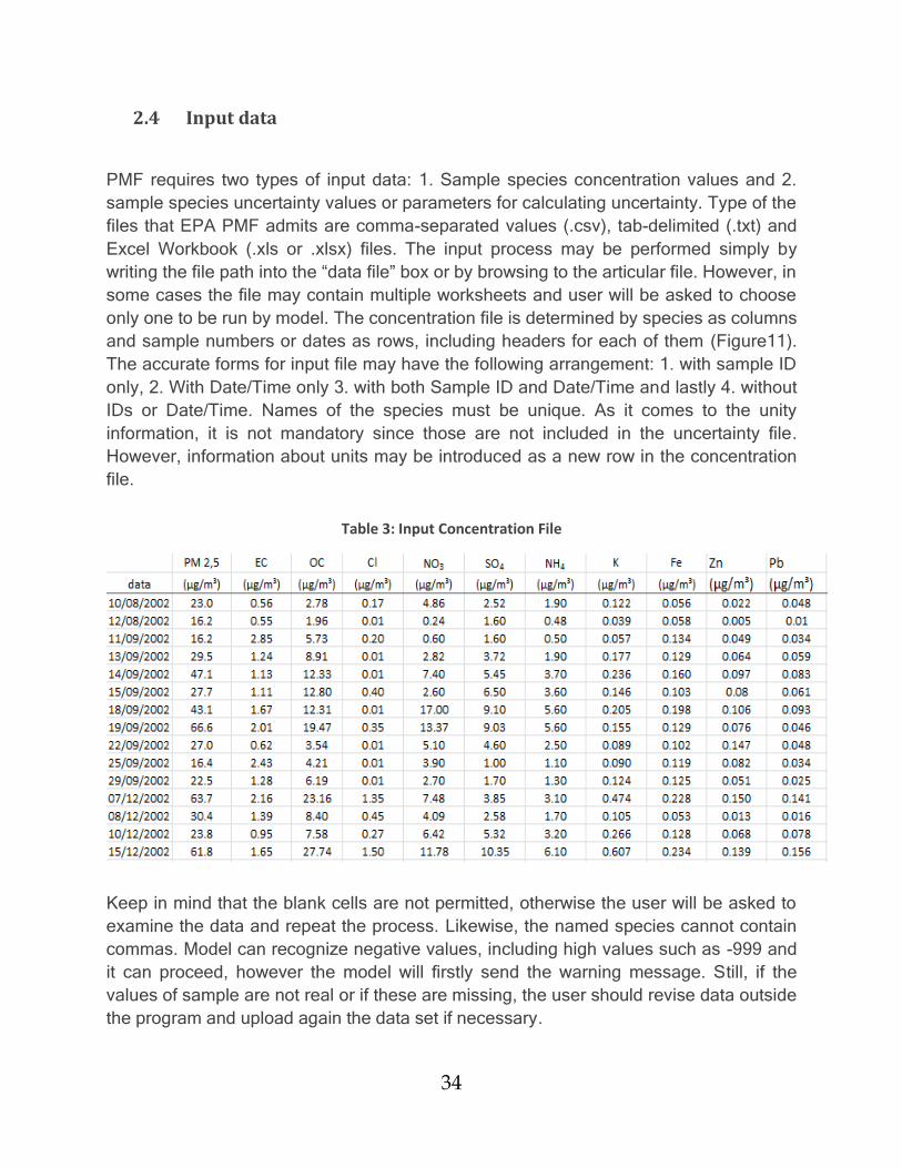
2.4 Input data

PMF requires two types of input data: 1. Sample species concentration values and 2.

sample species uncertainty values or parameters for calculating uncertainty. Type of the

files that EPA PMF admits are comma-separated values (.csv), tab-delimited (.txt) and

Excel Workbook (.xls or .xlsx) files. The input process may be performed simply by

writing the file path into the “data file” box or by browsing to the articular file. However, in

some cases the file may contain multiple worksheets and user will be asked to choose

only one to be run by model. The concentration file is determined by species as columns

and sample numbers or dates as rows, including headers for each of them (Figure11).

The accurate forms for input file may have the following arrangement: 1. with sample ID

only, 2. With Date/Time only 3. with both Sample ID and Date/Time and lastly 4. without

IDs or Date/Time. Names of the species must be unique. As it comes to the unity

information, it is not mandatory since those are not included in the uncertainty file.

However, information about units may be introduced as a new row in the concentration

file.

Table 3: Input Concentration File

Keep in mind that the blank cells are not permitted, otherwise the user will be asked to

examine the data and repeat the process. Likewise, the named species cannot contain

commas. Model can recognize negative values, including high values such as -999 and

it can proceed, however the model will firstly send the warning message. Still, if the

values of sample are not real or if these are missing, the user should revise data outside

the program and upload again the data set if necessary.

35

Sampling and analytical errors can be identified from the sample species uncertainties.

In some cases, analytical laboratory can provide an uncertainty assessment for each

value. Nonetheless, uncertainties are not always available, thus errors must be

estimated by the user.

Uncertainty files are being accepted by EPA PMF 5.0 in only two forms: 1. observation-

based and 2. equation-based. The first group is providing estimated information of the

uncertainty for each species in a sample. Dimensions should be the same as in the

concentration file, but should not include units. The program itself will check the

correspondence of the uncertainties file and the concentration file, and user will be

notified if some mismatches appear. Nonetheless, program will continue running if

encounters some minor mistake, but in a case of mismatching in the number of

samples, the program will not allow further evaluation of data. In the uncertainty file,

negative or zero values are not considered as relative values and must be excluded

from data set. If some values are present with stated values, PMF will show an error

message and the user will be asked to remove these values from the file and to reload

the uncertainty file.

Uncertainty file that contains species-specific parameters, the software EPA PMF 5.0

processes in order to calculate uncertainties for each sample. This file should contain

one row of species with their names. The row that follows should contain species-

specific method detection limit (MLD) that is accompanied by the row of uncertainties.

As stated before, zero and negative numbers are not permitted for both, detection limit

or for the uncertainty values (EPA Positive Matrix Factorization (PMF) 5.0.

Fundamentals and User Guide).

2.5 Output Data

The analyst can identify the output file, followed by the choice of the PMF output file

types and specify a prefix for the output files. The prefix is always added to the

beginning of every file, thus it will be always used as the first part of the output file.

Letters or numbers can be used in creation of the prefix, however other characters such

as “-” and “_” are not permitted. In a case that this prefix is not changed during the

succeeding run, a warming message will be showed.

After the base runs are finalized, the output files are created. These files contain all

necessary information for the on-screen display of the results. The number of the

created output files, depends mainly on the type of the output file chosen. Accordingly

the type of the output file may be:

36

Tab-delimited text (.txt)

Comma-separated variable (.csv) or

Excel Workbook (.xls)

If analyst choose Excel Workbook as an output file, two output files will be automatically

created by EPA PMF during base runs and will be preserved in the output folded that

was selected by analyst: *_base.xls and *_diagnostics.xls. These files are containing the

following information:

*_base.xls – Profiles, Contributions, Residual, Run Comparison

*_diagnostics.xls. – Summary, Input, Base Runs

On the other hand, if the analyst choses comma-separated variable (.csv), five output

files will be created: *_diag, *_contrib, *_profile, *_resid and *_run_comparison, where

each of the sections expresses the following information:

*_diag has an information of the user inputs and model diagnostic information

*_contrib has the contributions for the each base run which is used to create the

contribution graphs on the Profiles/Contributions tab. Run number is governing

the sorting of the contributions. Firstly shown are always normalized

contributions, and contributions in mass units is following if a total variable is

specified.

*_profile has the profiles for every base run which is used to create graphs on the

Profiles/Contributions tab. Like in the previous case, profiles are sorted by run

number, where profiles in mass units are shown first, followed by profiles in

percent of species and concentration fraction of species total if a total mass

variable is specified.

*_resid has the residuals, which are regulated and scaled by the uncertainty data

for every base run. It is used to create the graphs and tables on the residual

analysis screen.

*_run_comparison has a summary of the species distribution across all PMF runs

and for all factors and their comparison to the lowest Q (robust) run.

*_base has the *_contrib, *_profile, *_resid and *_run_comparison in the same

Excel Workbook, however in the separated worksheets.

Likewise, if a “.txt” type is selected, the information in the base runs tab is created as

separate file and the diagnostics tab information is merged into one file.

All output files are being saved to the directory previously specified “Output Folder”

section in the Data Files screen and with using the prefix defined in the “Output File

Prefix” section (EPA Positive Matrix Factorization (PMF) 5.0. Fundamentals and User

Guide).

37

2.6 Environmental Data

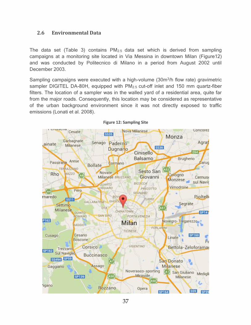
The data set (Table 3) contains PM2.5 data set which is derived from sampling

campaigns at a monitoring site located in Via Messina in downtown Milan (Figure12)

and was conducted by Politecnico di Milano in a period from August 2002 until

December 2003.

Sampling campaigns were executed with a high-volume (30m3/h flow rate) gravimetric

sampler DIGITEL DA-80H, equipped with PM2.5 cut-off inlet and 150 mm quartz-fiber

filters. The location of a sampler was in the walled yard of a residential area, quite far

from the major roads. Consequently, this location may be considered as representative

of the urban background environment since it was not directly exposed to traffic

emissions (Lonati et al. 2008).

Figure 12: Sampling Site

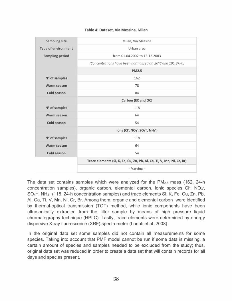
38

Table 4: Dataset, Via Messina, Milan

Sampling site Milan, Via Messina

Type of environment Urban area

Sampling period from 01.04.2002 to 13.12.2003

(Concentrations have been normalized at 20oC and 101.3kPa)

PM2.5

No of samples 162

Warm season 78

Cold season 84

Carbon (EC and OC)

No of samples 118

Warm season 64

Cold season 54

Ions (Cl-, NO3-, SO4

2-, NH4+)

No of samples 118

Warm season 64

Cold season 54

Trace elements (Si, K, Fe, Cu, Zn, Pb, Al, Ca, Ti, V, Mn, Ni, Cr, Br)

- Varying -

The data set contains samples which were analyzed for the PM2.5 mass (162, 24-h

concentration samples), organic carbon, elemental carbon, ionic species Cl-, NO3-,

SO42-, NH4

+ (118, 24-h concentration samples) and trace elements Si, K, Fe, Cu, Zn, Pb,

Al, Ca, Ti, V, Mn, Ni, Cr, Br. Among them, organic and elemental carbon were identified

by thermal-optical transmission (TOT) method, while ionic components have been

ultrasonically extracted from the filter sample by means of high pressure liquid

chromatography technique (HPLC). Lastly, trace elements were determined by energy

dispersive X-ray fluorescence (XRF) spectrometer (Lonati et al. 2008).

In the original data set some samples did not contain all measurements for some

species. Taking into account that PMF model cannot be run if some data is missing, a

certain amount of species and samples needed to be excluded from the study; thus,

original data set was reduced in order to create a data set that will contain records for all

days and species present.

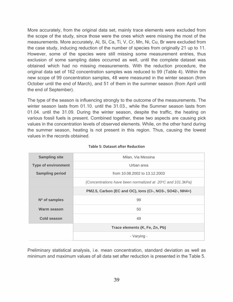
39

More accurately, from the original data set, mainly trace elements were excluded from

the scope of the study, since those were the ones which were missing the most of the

measurements. More accurately, Al, Si, Ca, Ti, V, Cr, Mn, Ni, Cu, Br were excluded from

the case study, inducing reduction of the number of species from originally 21 up to 11.

However, some of the species were still missing some measurement entries, thus

exclusion of some sampling dates occurred as well, until the complete dataset was

obtained which had no missing measurements. With the reduction procedure, the

original data set of 162 concentration samples was reduced to 99 (Table 4). Within the

new scope of 99 concentration samples, 48 were measured in the winter season (from

October until the end of March), and 51 of them in the summer season (from April until

the end of September).

The type of the season is influencing strongly to the outcome of the measurements. The

winter season lasts from 01.10. until the 31.03., while the Summer season lasts from

01.04. until the 31.09. During the winter season, despite the traffic, the heating on

various fossil fuels is present. Combined together, these two aspects are causing pick

values in the concentration levels of observed elements. While, on the other hand during

the summer season, heating is not present in this region. Thus, causing the lowest

values in the records obtained.

Table 5: Dataset after Reduction

Sampling site Milan, Via Messina

Type of environment Urban area

Sampling period from 10.08.2002 to 13.12.2003

(Concentrations have been normalized at 20oC and 101.3kPa)

PM2.5, Carbon (EC and OC), Ions (Cl-, NO3-, SO42-, NH4+)

No of samples 99

Warm season 50

Cold season 49

Trace elements (K, Fe, Zn, Pb)

- Varying -

Preliminary statistical analysis, i.e. mean concentration, standard deviation as well as

minimum and maximum values of all data set after reduction is presented in the Table 5.

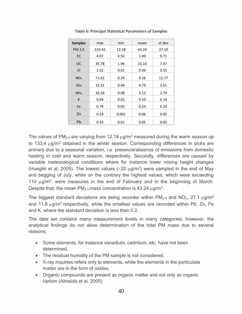
40

Table 6: Principal Statistical Parameters of Samples

Samples max min mean st.dev

PM 2,5 133.42 12.18 43.24 27.10

EC 4.97 0.50 1.49 0.71

OC 35.78 1.96 10.16 7.47

Cl 2.52 0.01 0.36 0.55

NO3 71.62 0.24 9.56 11.77

SO4 15.31 0.46 4.79 2.61

NH4 16.16 0.08 3.13 2.74

K 0.94 0.01 0.10 0.14

Fe 0.79 0.05 0.24 0.14

Zn 0.29 0.001 0.06 0.05

Pb 0.35 0.01 0.05 0.05

The values of PM2.5 are varying from 12.18 g/m3 measured during the warm season up

to 133,4 g/m3 obtained in the winter season. Corresponding differences in picks are

primary due to a seasonal variation, i.e. presence/absence of emissions from domestic

heating in cold and warm season, respectively. Secondly, differences are caused by

variable meteorological conditions where for instance lower mixing height changes

(Hueglin et al. 2005). The lowest values (20 g/m3) were sampled in the end of May

and begging of July, while on the contrary the highest values, which were exceeding

110 g/m3, were measures in the end of February and in the beginning of March.

Despite that, the mean PM2.5 mass concentration is 43.24 g/m3.

The biggest standard deviations are being recorder within PM2.5 and NO3, 27.1 g/m3

and 11.8 g/m3 respectively, while the smallest values are recorded within Pb, Zn, Fe

and K, where the standard deviation is less than 0.2.

The data set contains many measurement levels in many categories; however, the

analytical findings do not allow determination of the total PM mass due to several

reasons:

Some elements, for instance vanadium, cadmium, etc. have not been

determined,

The residual humidity of the PM sample is not considered,

X-ray inquiries refers only to elements, while the elements in the particulate

matter are in the form of oxides,

Organic compounds are present as organic matter and not only as organic

carbon (Almeida et al. 2005)

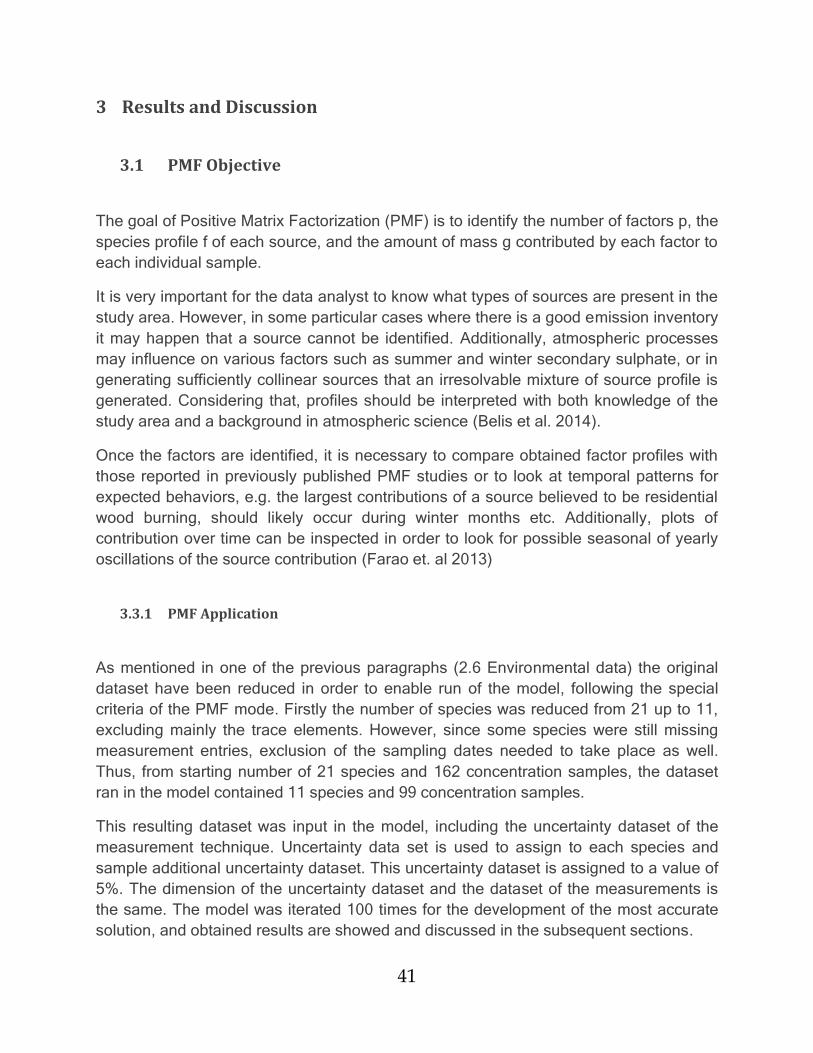
41

3 Results and Discussion

3.1 PMF Objective

The goal of Positive Matrix Factorization (PMF) is to identify the number of factors p, the

species profile f of each source, and the amount of mass g contributed by each factor to

each individual sample.

It is very important for the data analyst to know what types of sources are present in the

study area. However, in some particular cases where there is a good emission inventory

it may happen that a source cannot be identified. Additionally, atmospheric processes

may influence on various factors such as summer and winter secondary sulphate, or in

generating sufficiently collinear sources that an irresolvable mixture of source profile is

generated. Considering that, profiles should be interpreted with both knowledge of the

study area and a background in atmospheric science (Belis et al. 2014).

Once the factors are identified, it is necessary to compare obtained factor profiles with

those reported in previously published PMF studies or to look at temporal patterns for

expected behaviors, e.g. the largest contributions of a source believed to be residential

wood burning, should likely occur during winter months etc. Additionally, plots of

contribution over time can be inspected in order to look for possible seasonal of yearly

oscillations of the source contribution (Farao et. al 2013)

3.3.1 PMF Application

As mentioned in one of the previous paragraphs (2.6 Environmental data) the original

dataset have been reduced in order to enable run of the model, following the special

criteria of the PMF mode. Firstly the number of species was reduced from 21 up to 11,

excluding mainly the trace elements. However, since some species were still missing

measurement entries, exclusion of the sampling dates needed to take place as well.

Thus, from starting number of 21 species and 162 concentration samples, the dataset

ran in the model contained 11 species and 99 concentration samples.

This resulting dataset was input in the model, including the uncertainty dataset of the

measurement technique. Uncertainty data set is used to assign to each species and

sample additional uncertainty dataset. This uncertainty dataset is assigned to a value of

5%. The dimension of the uncertainty dataset and the dataset of the measurements is

the same. The model was iterated 100 times for the development of the most accurate

solution, and obtained results are showed and discussed in the subsequent sections.

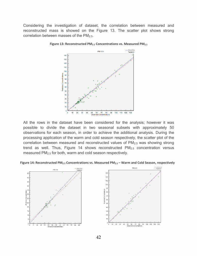
42

Considering the investigation of dataset, the correlation between measured and

reconstructed mass is showed on the Figure 13. The scatter plot shows strong

correlation between masses of the PM2.5.

Figure 13: Reconstructed PM2.5 Concentrations vs. Measured PM2.5

All the rows in the dataset have been considered for the analysis; however it was

possible to divide the dataset in two seasonal subsets with approximately 50

observations for each season, in order to achieve the additional analysis. During the

processing application of the warm and cold season respectively, the scatter plot of the

correlation between measured and reconstructed values of PM2.5 was showing strong

trend as well. Thus, Figure 14 shows reconstructed PM2.5 concentration versus

measured PM2.5 for both, warm and cold season respectively.

Figure 14: Reconstructed PM2.5 Concentrations vs. Measured PM2.5 – Warm and Cold Season, respectively

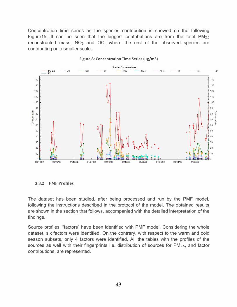
43

Concentration time series as the species contribution is showed on the following

Figure15. It can be seen that the biggest contributions are from the total PM2.5

reconstructed mass, NO3 and OC, where the rest of the observed species are

contributing on a smaller scale.

Figure 8: Concentration Time Series (g/m3)

3.3.2 PMF Profiles

The dataset has been studied, after being processed and run by the PMF model,

following the instructions described in the protocol of the model. The obtained results

are shown in the section that follows, accompanied with the detailed interpretation of the

findings.

Source profiles, “factors” have been identified with PMF model. Considering the whole

dataset, six factors were identified. On the contrary, with respect to the warm and cold

season subsets, only 4 factors were identified. All the tables with the profiles of the

sources as well with their fingerprints i.e. distribution of sources for PM2.5, and factor

contributions, are represented.

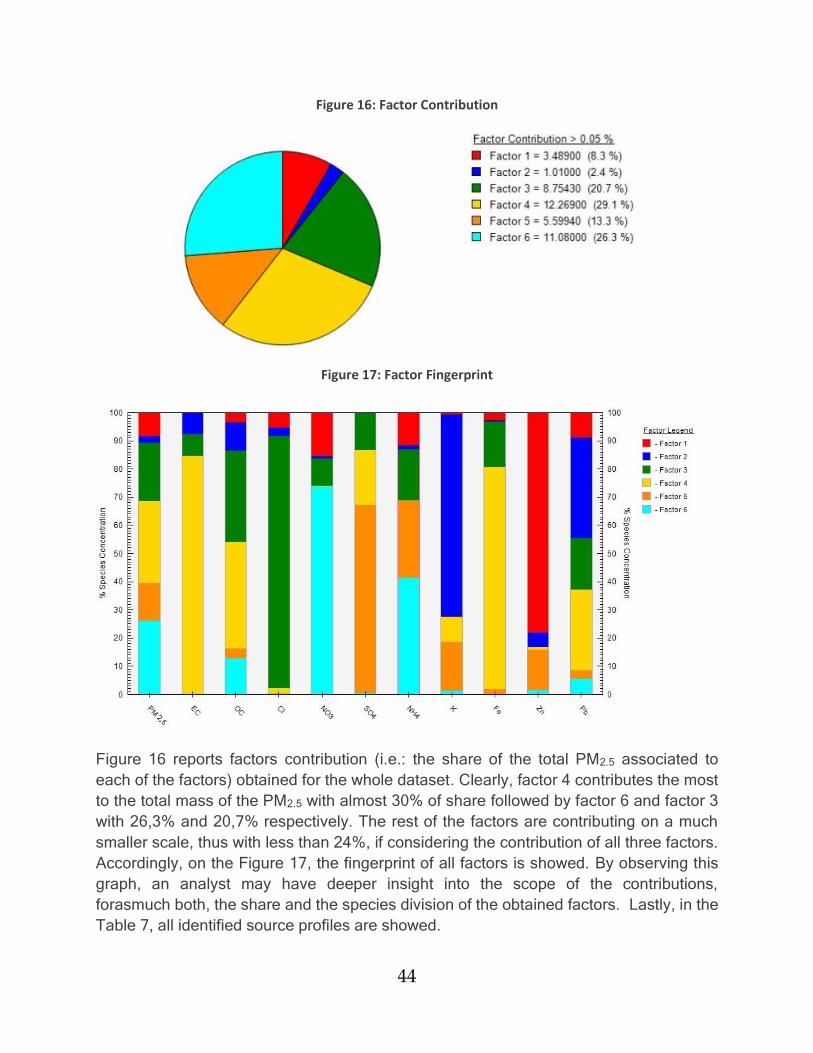
44

Figure 16: Factor Contribution

Figure 17: Factor Fingerprint

Figure 16 reports factors contribution (i.e.: the share of the total PM2.5 associated to

each of the factors) obtained for the whole dataset. Clearly, factor 4 contributes the most

to the total mass of the PM2.5 with almost 30% of share followed by factor 6 and factor 3

with 26,3% and 20,7% respectively. The rest of the factors are contributing on a much

smaller scale, thus with less than 24%, if considering the contribution of all three factors.

Accordingly, on the Figure 17, the fingerprint of all factors is showed. By observing this

graph, an analyst may have deeper insight into the scope of the contributions,

forasmuch both, the share and the species division of the obtained factors. Lastly, in the

Table 7, all identified source profiles are showed.

45

Table 7: Factor Profiles (g/m3)

Factor 2

Factor 3

Factor 4

Factor 5

Factor 6

Factor 1

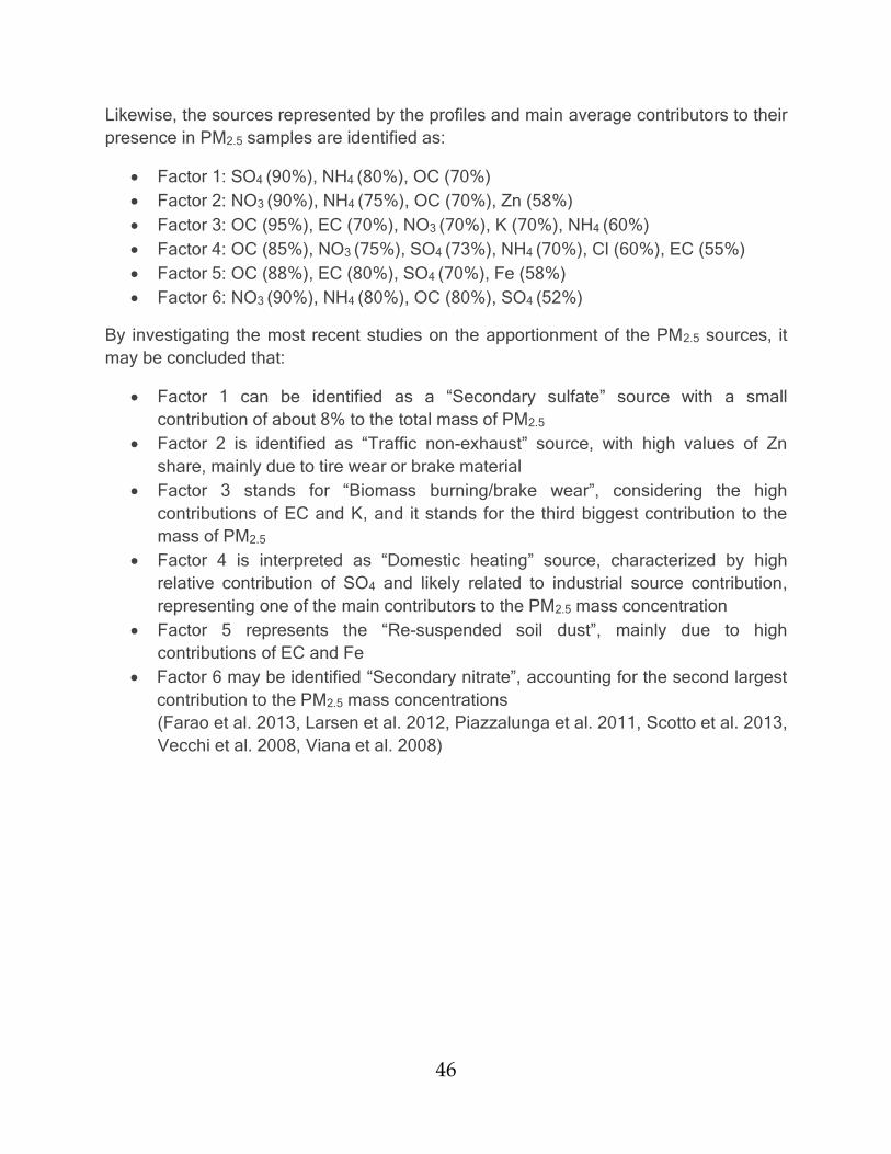
46

Likewise, the sources represented by the profiles and main average contributors to their

presence in PM2.5 samples are identified as:

Factor 1: SO4 (90%), NH4 (80%), OC (70%)

Factor 2: NO3 (90%), NH4 (75%), OC (70%), Zn (58%)

Factor 3: OC (95%), EC (70%), NO3 (70%), K (70%), NH4 (60%)

Factor 4: OC (85%), NO3 (75%), SO4 (73%), NH4 (70%), Cl (60%), EC (55%)

Factor 5: OC (88%), EC (80%), SO4 (70%), Fe (58%)

Factor 6: NO3 (90%), NH4 (80%), OC (80%), SO4 (52%)

By investigating the most recent studies on the apportionment of the PM2.5 sources, it

may be concluded that:

Factor 1 can be identified as a “Secondary sulfate” source with a small

contribution of about 8% to the total mass of PM2.5

Factor 2 is identified as “Traffic non-exhaust” source, with high values of Zn

share, mainly due to tire wear or brake material

Factor 3 stands for “Biomass burning/brake wear”, considering the high

contributions of EC and K, and it stands for the third biggest contribution to the

mass of PM2.5

Factor 4 is interpreted as “Domestic heating” source, characterized by high

relative contribution of SO4 and likely related to industrial source contribution,

representing one of the main contributors to the PM2.5 mass concentration

Factor 5 represents the “Re-suspended soil dust”, mainly due to high

contributions of EC and Fe

Factor 6 may be identified “Secondary nitrate”, accounting for the second largest

contribution to the PM2.5 mass concentrations

(Farao et al. 2013, Larsen et al. 2012, Piazzalunga et al. 2011, Scotto et al. 2013,

Vecchi et al. 2008, Viana et al. 2008)

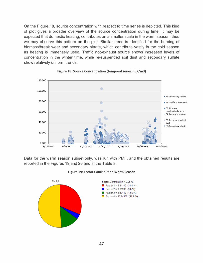
47

On the Figure 18, source concentration with respect to time series is depicted. This kind

of plot gives a broader overview of the source concentration during time. It may be

expected that domestic heating, contributes on a smaller scale in the warm season, thus

we may observe this pattern on the plot. Similar trend is identified for the burning of

biomass/break wear and secondary nitrate, which contribute vastly in the cold season

as heating is immensely used. Traffic not-exhaust source shows increased levels of

concentration in the winter time, while re-suspended soil dust and secondary sulfate

show relatively uniform trends.

Figure 18: Source Concentration (temporal series) (g/m3)

Data for the warm season subset only, was run with PMF, and the obtained results are

reported in the Figures 19 and 20 and in the Table 8.

Figure 19: Factor Contribution Warm Season

0.000

20.000

40.000

60.000

80.000

100.000

120.000

5/24/2002 9/1/2002 12/10/2002 3/20/2003 6/28/2003 10/6/2003 1/14/2004

F1: Secondary sulfate

F2: Traffic not-exhaust

F3: Biomassburning/brake wear

F4: Domestic heating

F5: Re-suspended soildust

F6: Secondary nitrate

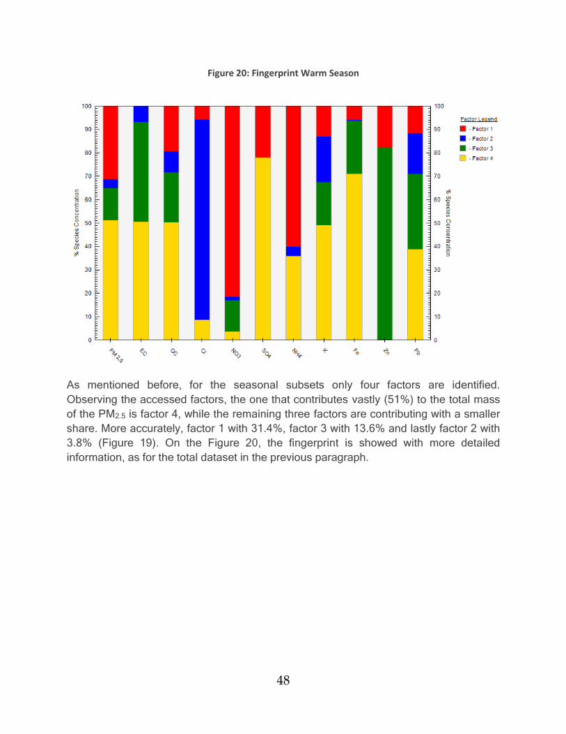
48

Figure 20: Fingerprint Warm Season

As mentioned before, for the seasonal subsets only four factors are identified.

Observing the accessed factors, the one that contributes vastly (51%) to the total mass

of the PM2.5 is factor 4, while the remaining three factors are contributing with a smaller

share. More accurately, factor 1 with 31.4%, factor 3 with 13.6% and lastly factor 2 with

3.8% (Figure 19). On the Figure 20, the fingerprint is showed with more detailed

information, as for the total dataset in the previous paragraph.

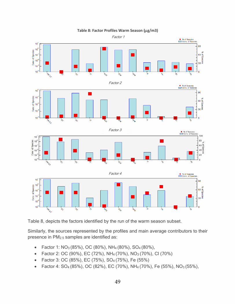
49

Table 8: Factor Profiles Warm Season (g/m3)

Table 8, depicts the factors identified by the run of the warm season subset.

Similarly, the sources represented by the profiles and main average contributors to their

presence in PM2.5 samples are identified as:

Factor 1: NO3 (85%), OC (80%), NH4 (80%), SO4 (80%),

Factor 2: OC (90%), EC (72%), NH4 (70%), NO3 (70%), Cl (70%)

Factor 3: OC (85%), EC (75%), SO4 (75%), Fe (55%)

Factor 4: SO4 (85%), OC (82%), EC (70%), NH4 (70%), Fe (55%), NO3 (55%),

Factor 1

Factor 2

Factor 3

Factor 4

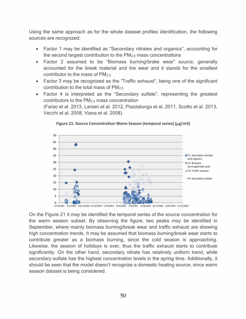
50

Using the same approach as for the whole dataset profiles identification, the following

sources are recognized:

Factor 1 may be identified as “Secondary nitrates and organics”, accounting for

the second largest contribution to the PM2.5 mass concentrations

Factor 2 assumed to be “Biomass burning/brake wear” source, generally

accounted for the break material and tire wear and it stands for the smallest

contributor to the mass of PM2.5

Factor 3 may be recognized as the “Traffic exhaust”, being one of the significant

contribution to the total mass of PM2.5

Factor 4 is interpreted as the “Secondary sulfate”, representing the greatest

contributors to the PM2.5 mass concentration

(Farao et al. 2013, Larsen et al. 2012, Piazzalunga et al. 2011, Scotto et al. 2013,

Vecchi et al. 2008, Viana et al. 2008)

Figure 21: Source Concentration Warm Season (temporal series) (g/m3)

On the Figure 21 it may be identified the temporal series of the source concentration for

the warm season subset. By observing the figure, two peaks may be identified in

September, where mainly biomass burning/break wear and traffic exhaust are showing

high concentration trends. It may be assumed that biomass burning/break wear starts to

contribute greater as a biomass burning, since the cold season is approaching.

Likewise, the season of holidays is over, thus the traffic exhaust starts to contribute

significantly. On the other hand, secondary nitrate has relatively uniform trend, while

secondary sulfate has the highest concentration levels in the spring time. Additionally, it

should be seen that the model doesn’t recognize a domestic heating source, since warm

season dataset is being considered.

0

5

10

15

20

25

30

35

40

45

50

7/13/2002 9/1/2002 10/21/2002 12/10/2002 1/29/2003 3/20/2003 5/9/2003 6/28/2003 8/17/2003 10/6/2003 11/25/2003

F1: Secondary nitratesand organics

F2: Biomassburning/break wear

F3: Traffic exhaust

F4: Secondary sulfate

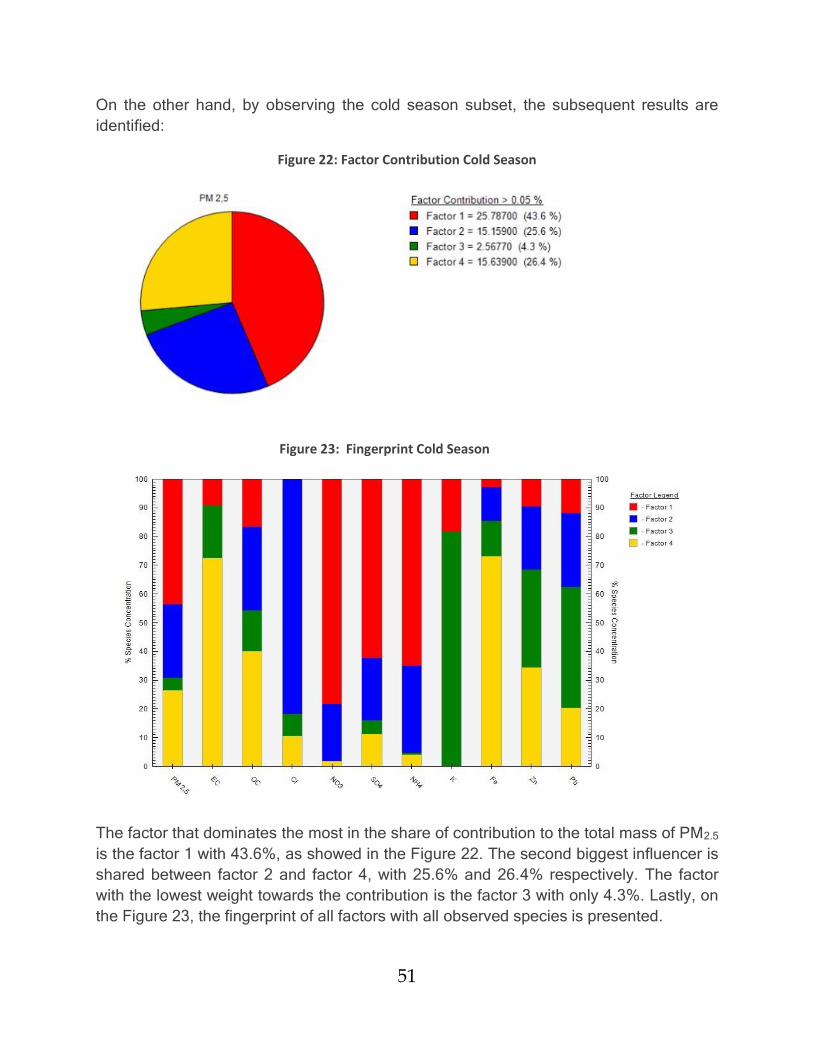
51

On the other hand, by observing the cold season subset, the subsequent results are

identified:

Figure 22: Factor Contribution Cold Season

The factor that dominates the most in the share of contribution to the total mass of PM2.5

is the factor 1 with 43.6%, as showed in the Figure 22. The second biggest influencer is

shared between factor 2 and factor 4, with 25.6% and 26.4% respectively. The factor

with the lowest weight towards the contribution is the factor 3 with only 4.3%. Lastly, on

the Figure 23, the fingerprint of all factors with all observed species is presented.

Figure 23: Fingerprint Cold Season

52

Table 9: Factor Profiles Cold Season (g/m3)

In the Table 9 obtained profiles for the cold season are depicted.

Additionally, the sources represented by the profiles and main average contributors to

their presence in PM2.5 samples are identified as:

Factor 1: SO4 (80%), NH4 (80%), OC (77%),

Factor 2: OC (85%), NO3 (85%), NH4 (78%), SO4 (75%), Cl (70%)

Factor 3: OC (90%), EC (75%), SO4 (75%), K (70%), Cl (60%), NH4 (55%),

K (55%)

Factor 4: OC (90%), EC (75%), SO4 (70%), NO3 (65%), NH4 (60%), Fe (60%),

Factor 1

Factor 2

Factor 3

Factor 4

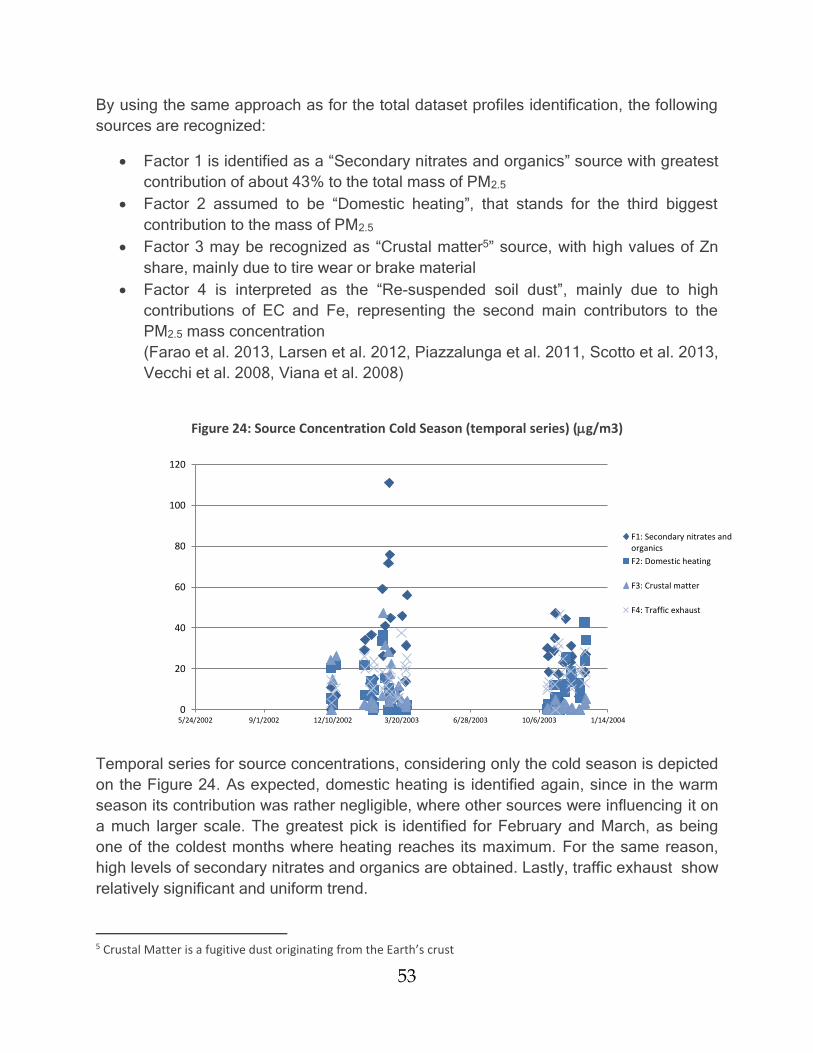
53

By using the same approach as for the total dataset profiles identification, the following

sources are recognized:

Factor 1 is identified as a “Secondary nitrates and organics” source with greatest

contribution of about 43% to the total mass of PM2.5

Factor 2 assumed to be “Domestic heating”, that stands for the third biggest

contribution to the mass of PM2.5

Factor 3 may be recognized as “Crustal matter5” source, with high values of Zn

share, mainly due to tire wear or brake material

Factor 4 is interpreted as the “Re-suspended soil dust”, mainly due to high

contributions of EC and Fe, representing the second main contributors to the

PM2.5 mass concentration

(Farao et al. 2013, Larsen et al. 2012, Piazzalunga et al. 2011, Scotto et al. 2013,

Vecchi et al. 2008, Viana et al. 2008)

Figure 24: Source Concentration Cold Season (temporal series) (g/m3)

Temporal series for source concentrations, considering only the cold season is depicted

on the Figure 24. As expected, domestic heating is identified again, since in the warm

season its contribution was rather negligible, where other sources were influencing it on

a much larger scale. The greatest pick is identified for February and March, as being

one of the coldest months where heating reaches its maximum. For the same reason,

high levels of secondary nitrates and organics are obtained. Lastly, traffic exhaust show

relatively significant and uniform trend.

5 Crustal Matter is a fugitive dust originating from the Earth’s crust

0

20

40

60

80

100

120

5/24/2002 9/1/2002 12/10/2002 3/20/2003 6/28/2003 10/6/2003 1/14/2004

F1: Secondary nitrates andorganics

F2: Domestic heating

F3: Crustal matter

F4: Traffic exhaust

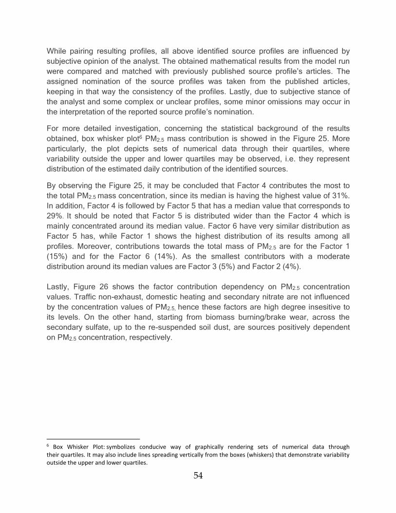
54

While pairing resulting profiles, all above identified source profiles are influenced by

subjective opinion of the analyst. The obtained mathematical results from the model run

were compared and matched with previously published source profile’s articles. The

assigned nomination of the source profiles was taken from the published articles,

keeping in that way the consistency of the profiles. Lastly, due to subjective stance of

the analyst and some complex or unclear profiles, some minor omissions may occur in

the interpretation of the reported source profile’s nomination.

For more detailed investigation, concerning the statistical background of the results

obtained, box whisker plot6 PM2.5 mass contribution is showed in the Figure 25. More

particularly, the plot depicts sets of numerical data through their quartiles, where

variability outside the upper and lower quartiles may be observed, i.e. they represent

distribution of the estimated daily contribution of the identified sources.

By observing the Figure 25, it may be concluded that Factor 4 contributes the most to

the total PM2.5 mass concentration, since its median is having the highest value of 31%.

In addition, Factor 4 is followed by Factor 5 that has a median value that corresponds to

29%. It should be noted that Factor 5 is distributed wider than the Factor 4 which is

mainly concentrated around its median value. Factor 6 have very similar distribution as

Factor 5 has, while Factor 1 shows the highest distribution of its results among all

profiles. Moreover, contributions towards the total mass of PM2.5 are for the Factor 1

(15%) and for the Factor 6 (14%). As the smallest contributors with a moderate

distribution around its median values are Factor 3 (5%) and Factor 2 (4%).

Lastly, Figure 26 shows the factor contribution dependency on PM2.5 concentration

values. Traffic non-exhaust, domestic heating and secondary nitrate are not influenced

by the concentration values of PM2.5, hence these factors are high degree insesitive to

its levels. On the other hand, starting from biomass burning/brake wear, across the

secondary sulfate, up to the re-suspended soil dust, are sources positively dependent

on PM2.5 concentration, respectively.

6 Box Whisker Plot: symbolizes conducive way of graphically rendering sets of numerical data through their quartiles. It may also include lines spreading vertically from the boxes (whiskers) that demonstrate variability outside the upper and lower quartiles.

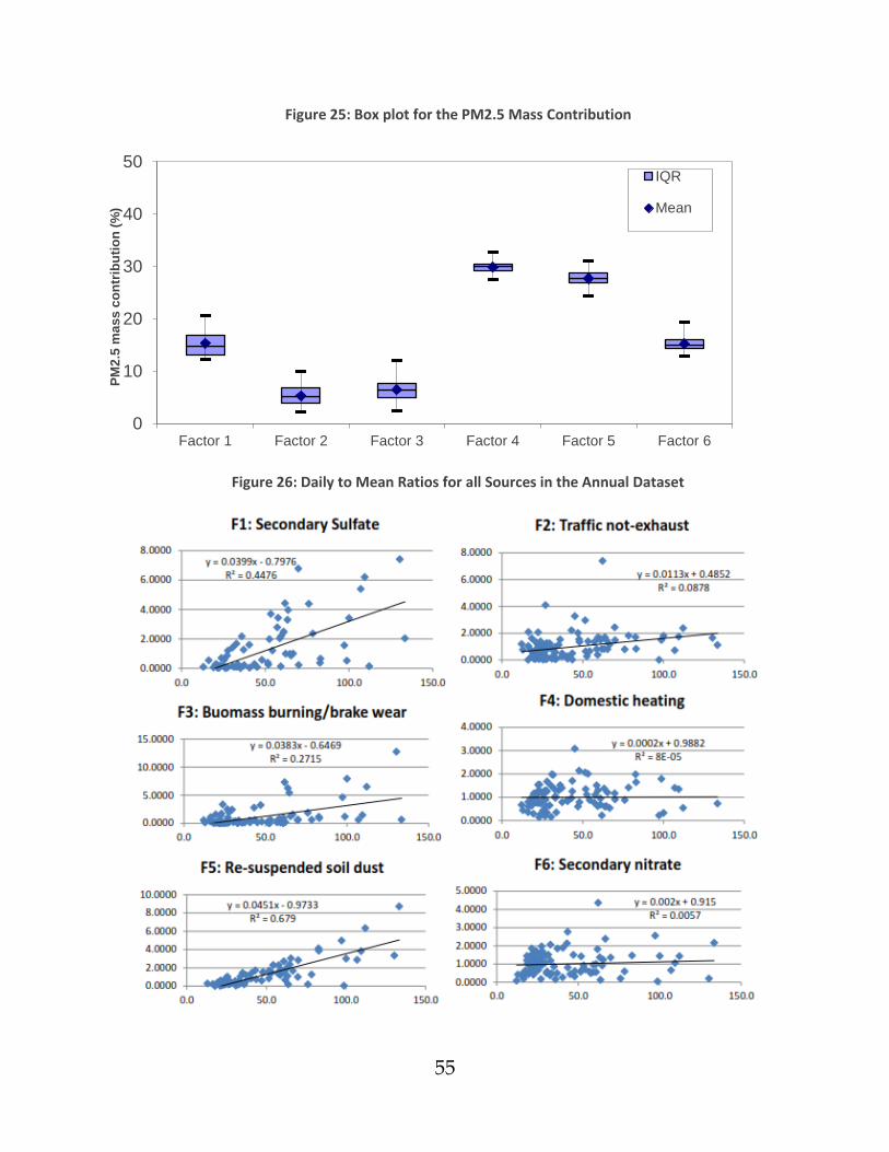
55

Figure 25: Box plot for the PM2.5 Mass Contribution

Figure 26: Daily to Mean Ratios for all Sources in the Annual Dataset

0

10

20

30

40

50

Factor 1 Factor 2 Factor 3 Factor 4 Factor 5 Factor 6

PM

2.5

ma

ss

co

ntr

ibu

tio

n (

%)

IQR

Mean

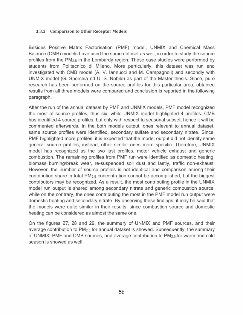
56

3.3.3 Comparison to Other Receptor Models

Besides Positive Matrix Factorisation (PMF) model, UNMIX and Chemical Mass

Balance (CMB) models have used the same dataset as well, in order to study the source

profiles from the PM2.5 in the Lombardy region. These case studies were performed by

students from Politecnico di Milano. More particularly, this dataset was run and

investigated with CMB model (A. V. Iannucci and M. Campagnoli) and secondly with

UNMIX model (G. Sporchia nd U. S. Nobile) as part of the Master thesis. Since, pure

research has been performed on the source profiles for this particular area, obtained

results from all three models were compared and conclusion is reported in the following

paragraph.

After the run of the annual dataset by PMF and UNMIX models, PMF model recognized

the most of source profiles, thus six, while UNMIX model highlighted 4 profiles. CMB

has identified 4 source profiles, but only with respect to seasonal subset; hence it will be

commented afterwards. In the both models output, ones relevant to annual dataset,

same source profiles were identified, secondary sulfate and secondary nitrate. Since,

PMF highlighted more profiles, it is expected that the model output did not identify same

general source profiles, instead, other similar ones more specific. Therefore, UNMIX

model has recognized as the two last profiles, motor vehicle exhaust and generic

combustion. The remaining profiles from PMF run were identified as domestic heating,

biomass burning/break wear, re-suspended soil dust and lastly, traffic non-exhaust.

However, the number of source profiles is not identical and comparison among their

contribution share in total PM2.5 concentration cannot be accomplished, but the biggest

contributors may be recognized. As a result, the most contributing profile in the UNMIX

model run output is shared among secondary nitrate and generic combustion source,

while on the contrary, the ones contributing the most in the PMF model run output were

domestic heating and secondary nitrate. By observing these findings, it may be said that

the models were quite similar in their results, since combustion source and domestic

heating can be considered as almost the same one.

On the figures 27, 28 and 29, the summary of UNMIX and PMF sources, and their

average contribution to PM2.5 for annual dataset is showed. Subsequently, the summary

of UNMIX, PMF and CMB sources, and average contribution to PM2.5 for warm and cold

season is showed as well.

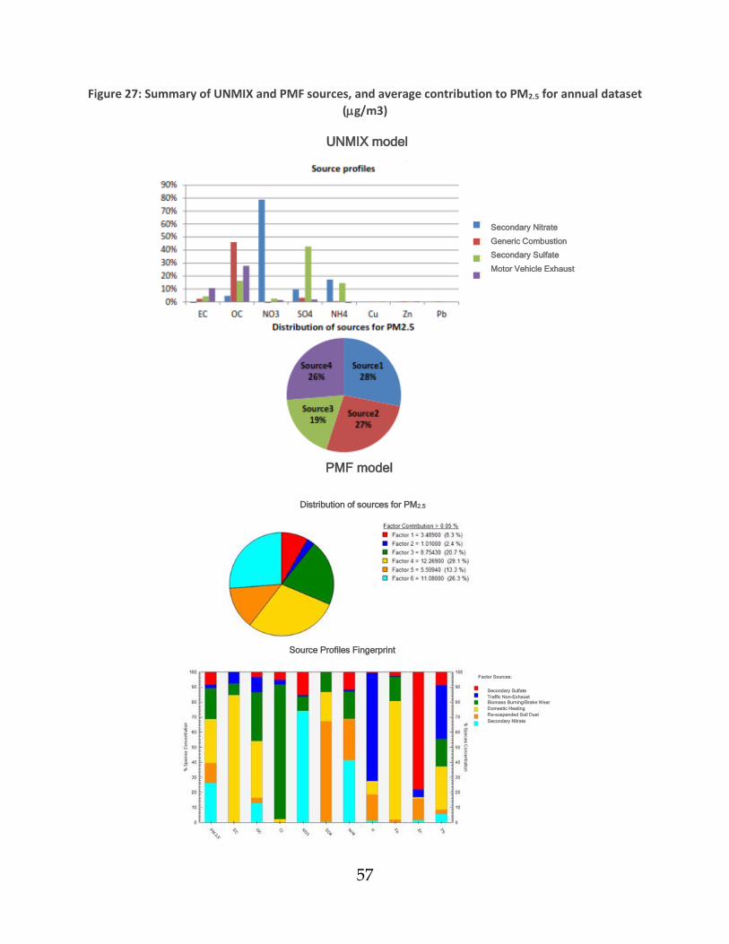
57

Figure 27: Summary of UNMIX and PMF sources, and average contribution to PM2.5 for annual dataset

(g/m3)

Secondary Sulfate

Traffic Non-Exhaust Biomass Burning/Brake Wear

Domestic Heating

Re-suspended Soil Dust

Secondary Nitrate

UNMIX model

PMF model

Distribution of sources for PM2.5

Source Profiles Fingerprint

Secondary Nitrate

Generic Combustion

Secondary Sulfate

Motor Vehicle Exhaust

Factor Sources:

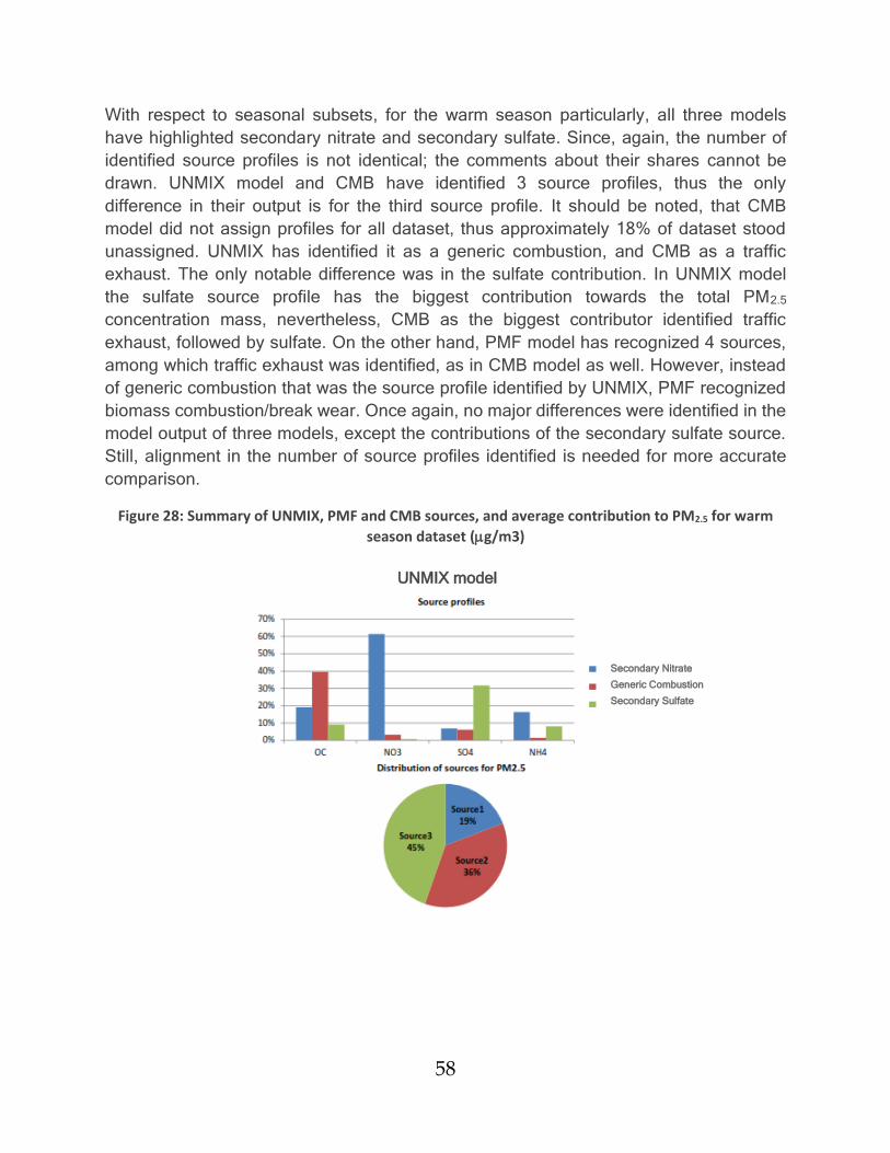
58

With respect to seasonal subsets, for the warm season particularly, all three models

have highlighted secondary nitrate and secondary sulfate. Since, again, the number of

identified source profiles is not identical; the comments about their shares cannot be

drawn. UNMIX model and CMB have identified 3 source profiles, thus the only

difference in their output is for the third source profile. It should be noted, that CMB

model did not assign profiles for all dataset, thus approximately 18% of dataset stood

unassigned. UNMIX has identified it as a generic combustion, and CMB as a traffic

exhaust. The only notable difference was in the sulfate contribution. In UNMIX model

the sulfate source profile has the biggest contribution towards the total PM2.5

concentration mass, nevertheless, CMB as the biggest contributor identified traffic

exhaust, followed by sulfate. On the other hand, PMF model has recognized 4 sources,

among which traffic exhaust was identified, as in CMB model as well. However, instead

of generic combustion that was the source profile identified by UNMIX, PMF recognized

biomass combustion/break wear. Once again, no major differences were identified in the

model output of three models, except the contributions of the secondary sulfate source.

Still, alignment in the number of source profiles identified is needed for more accurate

comparison.

Figure 28: Summary of UNMIX, PMF and CMB sources, and average contribution to PM2.5 for warm

season dataset (g/m3)

UNMIX model

Secondary Nitrate

Generic Combustion

Secondary Sulfate

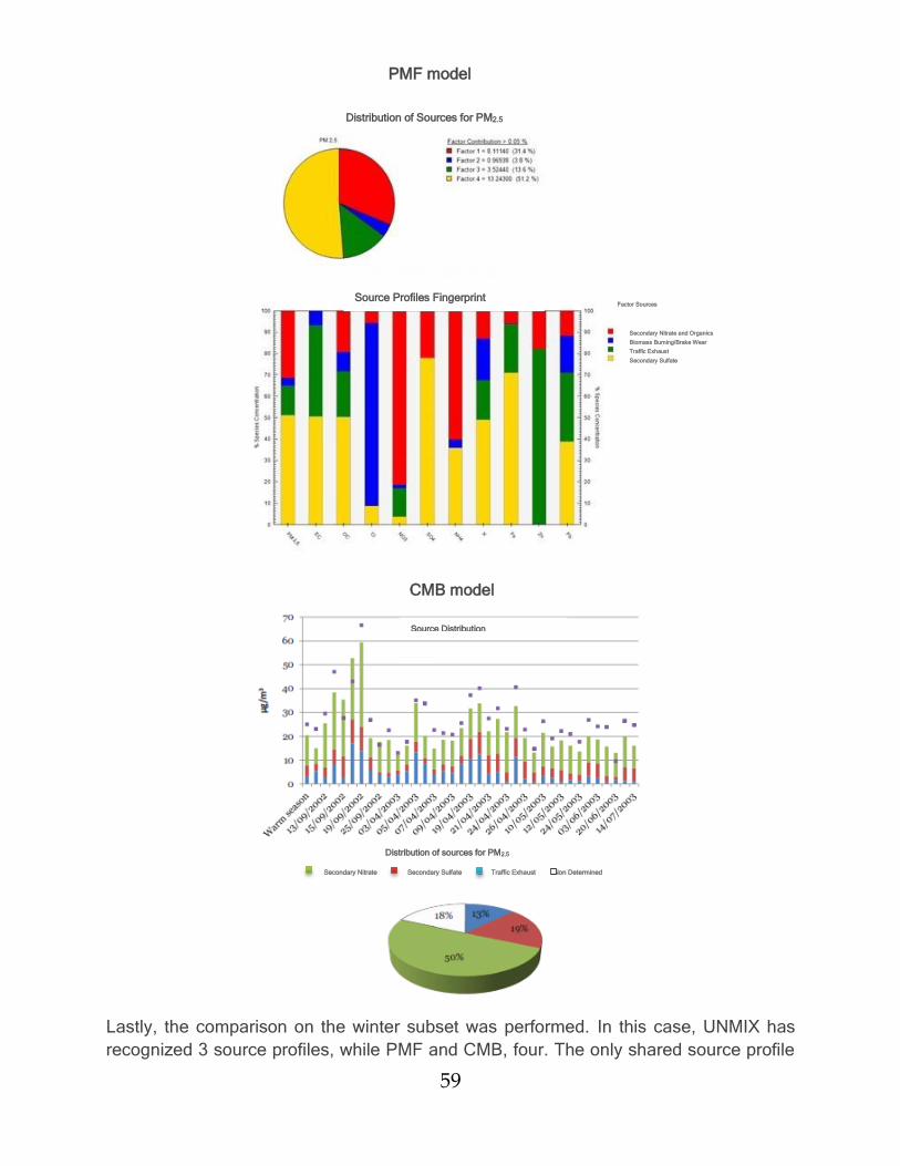
59

Lastly, the comparison on the winter subset was performed. In this case, UNMIX has

recognized 3 source profiles, while PMF and CMB, four. The only shared source profile

PMF model

Distribution of Sources for PM2.5

Source Profiles Fingerprint

Distribution of sources for PM2.5

CMB model

Source Distribution

Secondary Nitrate and Organics

Biomass Burning/Brake Wear

Traffic Exhaust

Secondary Sulfate

Factor Sources

Secondary Nitrate Secondary Sulfate Traffic Exhaust Non Determined

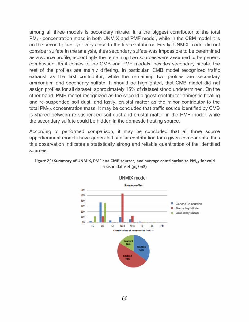
60

among all three models is secondary nitrate. It is the biggest contributor to the total

PM2.5 concentration mass in both UNMIX and PMF model, while in the CBM model it is

on the second place, yet very close to the first contributor. Firstly, UNMIX model did not

consider sulfate in the analysis, thus secondary sulfate was impossible to be determined

as a source profile; accordingly the remaining two sources were assumed to be generic

combustion. As it comes to the CMB and PMF models, besides secondary nitrate, the

rest of the profiles are mainly differing. In particular, CMB model recognized traffic

exhaust as the first contributor, while the remaining two profiles are secondary

ammonium and secondary sulfate. It should be highlighted, that CMB model did not

assign profiles for all dataset, approximately 15% of dataset stood undetermined. On the

other hand, PMF model recognized as the second biggest contributor domestic heating

and re-suspended soil dust, and lastly, crustal matter as the minor contributor to the

total PM2.5 concentration mass. It may be concluded that traffic source identified by CMB

is shared between re-suspended soil dust and crustal matter in the PMF model, while

the secondary sulfate could be hidden in the domestic heating source.

According to performed comparison, it may be concluded that all three source

apportionment models have generated similar contribution for a given components; thus

this observation indicates a statistically strong and reliable quantitation of the identified

sources.

Figure 29: Summary of UNMIX, PMF and CMB sources, and average contribution to PM2.5 for cold

season dataset (g/m3)

UNMIX model

Generic Combustion

Secondary Nitrate

Secondary Sulfate

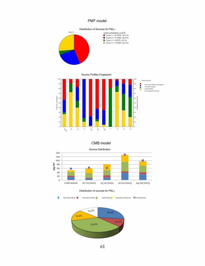
61

Source Profiles Fingerprint

Distribution of Sources for PM2.5

PMF model

CMB model

Source Distribution

Distribution of sources for PM2.5

Factor Sources

Secondary Nitrate and Organics

Domestic Heating

Crustal Matter

Re-suspended Soil Dust

Secondary Nitrate Secondary Sulfate Traffic Exhaust Secondary Ammonium Non Determined

62

Conclusion

Particulate matter as being one of the air pollutants is on its rising trend of growing

attention. Why? Particulate matter is well-known to its great potential for global warming

and harmful effects on human health and the environment. What is worsening the

situation is that these effects do not occur on the local scale only, but the global as well.

World leading organizations for health are trying to raise awareness that PM affects

human health more than any other pollutant, mainly towards the respiratory and

cardiovascular system. Accordingly, it is noted that recently vast amount of scientific

literature is investigating epidemiological, clinical and toxicological subjects. These

study cases identified an immense scale of adverse health effects, starting from

significant respiratory problems up to the cardiopulmonary adverse diseases and lung

cancer. The severity of its impact is connected to the concentration levels in the

atmospheric air, chemical composition, particle size distribution, duration of the

exposure, and individual sensitivity. These studies draw a conclusion that these effects

are caused by both, short-term and long-term exposure to particulate matter usually

inhaled within the urban areas throughout the world. World Health Organisation states

that particulate matter and effects that it causes, triggers death of about 0.85 million

people annually, mainly in the developing countries.

On the other hand, particulate matter’s influence on the environment it rather obvious.

Fossil combustion creates fumes and vapours that are reducing visibility, while besides

that, due to its chemical and physical characteristics, it influences the alteration of the

radiative balance of the atmosphere’s absorbing and reflecting solar radiation. Albedo,

known as the reflectivity of the Earth’s surface is reduced as well, mainly because of the

global warming phenomenon, i.e. reduction of snow and ice (surfaces that have the

most potent reflective power). Particulate matter that is suspended in the air creates fog,

mainly in the urban areas, but contributes vastly to the cloud’s creation as well. Clouds

are formed when condensation nuclei is created, around which the water droplet forms.

When the rain is created from these clouds, it may effect in forming strong fog or acid

rain that will have a severe effects of corrosion on the flora and fauna, buildings,

monuments and damage electrical installations. Additionally, the concentration of these

particles may influence greatly on the rainfall regime. On the other hand, earth’s climate

is immensely influenced by the type and concentration of particulate matter. Firstly, its

presence is driving global warming on a wide range, where some of the particles have

enormously large global warming potential. However, that is not the only impact on the

earth’s climate. As mentioned before, it is very important to control levels of the Earth’s

reflectivity. Particulate matter as reflective substance is helping to decrease temperature

on the earth with its shielding effects on the sunlight, but it keeps reflected infrared

radiation below its layer as well.

63

Severity of the impacts that air pollution has, became more than apparent when report

from European Environmental Agency was released. It claimed that dirty air cost society

189 billion euros a year; thus campaigners have demanded a crackdown on Europe’s

worst polluters. Referring to data from the EEA report, half of the damage is being done

by only one percent of industrial plants. Coal-fired power plants and the air pollution that

they emit, cost Europe approximately 189 billion euros in 2012., According to EEA

figures, among all European countries, Germany was Europe’s biggest contributor, It

has generated 38.2 billion euros of damage to society as a result of air pollution.

Subsequent country was the United Kingdom with 25.9 billion euros, followed by Poland

(24.8 billion euros), France (14.3 billion euros) and Italy (13.8 billion euros). As

expected, from the 30 most damaging facilities in Europe, eight were in Germany, six in

Poland, four in Romania, three in Bulgaria and the United Kingdom, two in Greece, and

one in the Czech Republic, Estonia, Italy and Slovakia.

Decision makers, in order to create effective strategies to control of reduce impacts on

the air quality, mainly use findings of the contributions of the various emission sources

to the particulate matter concentration levels. Scientific technique that examines this

phenomenon is called source apportionment. This technique is having two approaches,

receptor-oriented and source-oriented. Unlike other air model, receptor model do not

use pollutant emissions, meteorological data and chemical transformation mechanism.

Alternatively, receptor model uses chemical and physical characteristics of gases and

particles measured at source and receptor to identify both, presence and contribution of

sources to receptor concentrations. Since, the dataset used for this case study

contained concentrations levels and chemical specification of the particulate matter that

was sampled at a receptor (site) location, the used model was receptor-oriented. The

main objective of the model is to identify and quantify the sources of air pollutants at a

receptor location, their profiles and their relative contribution to the total particulate

matter concentrations.

Receptor models were developed in the United States and are vastly used to solve air

quality problems. Accordingly, the EPA7 has developed several receptor models in order

to reinforce the air quality management. The ones currently available are Chemical

Mass Balance (CMB), UNMIX and Positive Matrix Factorisation (PMF). This case study

was examined by the PMF receptor model. PMF represents a multivariate factor

analysis program that decomposes a matrix of identified data set into two matrices,

factor contributions and factor profiles. These factor profiles needs to be studied by the

user in order to allocate the source types that may be influencing to the same cluster, by

using quantified source profile information and emissions of discharge registers.

The fundamental objective of this work is to give contribution to better understanding of

the nature of particulate matter and to quantify relative significance of diverse emission 7 EPA - US Environmental Protective Agency

64

sources and enable decision makers to convey efficient air quality remediation plans.

Thus, the scope of this work is to perform a particulate matter source apportionment by

means of the PMF model on the particulate matter data set from Milan. The main focus

is on PM2.5, since recent air quality standards for particulate matter inquired by

European Union, studies also PM2.5, besides PM10, where were specified both,

concentration limits and an exposure reduction target. The second reason for

centralizing on PM2.5 is that anthropogenic carbon forms are almost completely included

in fine particulate matter.

The original dataset have been reduced in order to enable run of the model, following

the special criteria of the PMF model. Firstly the number of species was reduced from

21 up to 11, excluding mainly the trace elements. However, since some species were

still missing measurement entries, exclusion of the sampling dates needed to take place

as well. Thus, from starting number of 21 species and 162 concentration samples, the

dataset ran in the model contained 11 species and 99 concentration samples. The

investigation was firstly made at the whole dataset. Afterwards the data was separated

into warm and cold season subsets, where additional investigation was made.

For what concerns the annual dataset of PM2.5 in Milan, the simulation by PMF model

generated 6 sources (secondary sulfate, traffic non-exhaust, biomass burning/brake

wear, domestic heating, re-suspended soil dust, secondary nitrate) with average

contribution to the total PM2.5 mass that ranges between 10% and 20%, and as

expected, significant daily variability is identified. In particular, the main contributor is

identified as the domestic heating (29.1%). The one that follows is a secondary nitrate

(26.3%). These two finding are more than likely to be found, since the sampling area

represents very populated urban area, where great amounts of fossil fuels are being

combusted. The remaining sources are biomass burning/brake wear (20.7%), re-

suspended soil dust (13.3%), secondary sulfate (8.3%) and lastly, traffic non-exhaust

(2.4%) source. On the plot of time series, it was identified that domestic heating

contributes on a smaller scale in the warm season. Similar trend is identified for the

burning of biomass/break wear and secondary sulfate, which contribute vastly in the

cold season as heating is immensely used. Re-suspended soil dust shows the biggest

contribution in between the cold and warm season, while traffic non-exhaust and

secondary nitrate, show the similar, relatively uniform trend, with picks in September.

The sources were identified by comparing obtained relative contributions with results

acquired from previous studies.

On the seasonal basis, the number of sources identified for both seasons were four.

However, the type of sources identified, vary from season to season. The warm season

highlighted, secondary nitrate and organics, biomass burning/brake wear, traffic exhaust

and lastly secondary sulfate. On the contrary, the cold season obtained slightly different

results: secondary nitrates and organics, domestic heating, crustal matter and traffic

65

exhaust. Domestic heating draws immediate attention as it is appearing only in the cold

season, from apparent reason of the cold weather. On the other hand, traffic exhaust is

present in both seasons, where it greatly contributes to the total PM2.5. That trend should

draw attention of the decision makers to convey strict control and try to reduce the

strong impact from this source. For the concern of the average contribution to the PM2.5

mass concentration, two sources are contributing the most in the warm season:

secondary sulfate (51.2%) and secondary nitrate and organics (31.4%). The ones that

follow are contributing on the much smaller scale, traffic exhaust (13.6%) and biomass

burning/brake wear (3.8%). As for the cold season, out of four sources, three are

contributing with the great shares: secondary nitrates and organics (43.6), traffic

exhaust (26.4%) and lastly domestic heating (25.6%). The smallest contribution is

identified in the crustal matter (4.3%).

Due to the model structure, it is not possible to make more detailed distinction on the

type of combustion. Still, some important sources were recognized and this information

may be used to raise awareness as well to create some strategies with an aim to

improve the air quality of the area. Looking more into results obtained, it may be

concluded that the traffic exhaust contributes as double as in the warm season, growth

that may be associated with reduced traffic during summer months. By investigating

cold seasons, it can be remarked that no secondary sulfate source has been identified.

The reason for if may be in a fact that lower temperatures do not favour formation of the

sulfate. On the other hand, as expected, the combustion contribution is much higher in

the cold than in the warm season, mainly due to the domestic heating emissions. Lastly,

there is a slight change in contribution of secondary nitrates and organics from warm

season to cold one. Nitrate is having a higher volatility at higher temperatures, thus its

contribution is reduced in the warm season.

66

67

Literature

A. C. Rohr, R. E. Wyzga, “Attributing Health Effects to Individual Particulate Matter

Constituents” (2012), Atmospheric Environment 62, 130-152

A. D. Nazelle, M. J. Nieuwenhuijsen, J. M. Antó, M. Brauer, D. Briggs, C. Braun-

Fahrlander, N. Cavill, A. R. Cooper, H. Desqueyroux, S. Fruin, G. Hoek, L. Panis, N.

Janssen, M. Jerrett, M. Joffe, Z. J. Andersen, E. V. Kempen, S. Kingham, N. Kubesch, K.

M. Leyden, J. D. Marshall, “Improving Health Through Policies that Promote Active

Travel: A Review of Evidence to Support Integrated Health Impact Assessment” (2011),

Environment International 37, 766-777

A. V. Iannucci, M. Campanoli, “PM2.5 and PM10 Source Apportionment in Lombardy by

Chemical Mass Balance Receptor Modelling” (2012), Master Graduation Thesis,

Politecnico di Milano

A. Piazzalunga, V. Bernardoni, P. Fermo, G. Valli, R. Vecchi, “Wood Combustion

Contribution to PM: Results of Five Years Campaigns (2005-2009) in Lombardy Italy”

(2011), 10th International Conference on Carbonaceous Particles in the Atmosphere

B. R. Larsen, S. Gilardoni, K. Stenstrom, J. Niekzialek, J. Jimanez, C.A. Belis, “Sources

for PM Air Pollution in the Po Plain, Italy: II. Probabilistic Uncertainty Characterization

and Sensitivity Analysis of Secondary and Primary Sources” (2012), Atmospheric

Environment, 203-213

C. Hueglin, R. Gehrig, U. Baltensperger, M. Gysel, C. Monn, H. Vonmont, “Chemical

Characterization of PM2.5, PM10 and Coarse Particles at Urban, near City and Rural Sites

in Switzerland” (2005), Atmospheric Environment 39, 637–651

C. Farao, S. Canepari, C. Perrino, R. M. Harrison, “Sources of PM in an Industrial Area:

Comparison between Receptor Model Results and Semi-Empirical Calculations of

Source Contributions, Aerosol and Air Quality Research” (2013), Taiwan Association for

Aerosol Research

C. A. Belis, B. R. Larsen, F. Amato, I. E. Hadad, O. Favez, R. M. Harrison, P. K. Hoplke,

S. Nava, P. Paatero, A. Prévôt, U. Quass, R. Vecchi, M. Viana, “European Guide on Air

Pollution Source Apportionment with Receptor Models” (2014), JRC (Joint Research

Centre)

D. Mooibroek, M. Schaap, E. P. Weijers, R. Hoogerbrugge, “Source Apportionment and

Spatial Variability of PM2.5 using Measurements at Five Sites in the Netherlands” (2011),

Atmospheric Environment 45, 4180-4191

D. A. Thornhill, A. E. Williams, T. B. Onasch, E. Wood, S. C. Herndon, C. E. Kolb, W. B.

Knighton, M. Zavala, L. T. Molina, L. C. Marr, “Application of Positive Matrix Factorization

to On-Road Measurements for Source Apportionment of Diesel and Gasoline Powered

Vehicle Emissions in Mexico City” (2010), Atmospheric Chemical Physics 10, 3629-3644

D. Al-Ajmi, P. Zanetti, “An Introduction to Air Pollution – Definitions, Classifications and

History” (2007), Ambient Air Pollution, Chapter 1

E.G. Stephanou, “Aerosols PM10 and PM2.5” (2012) Volume 1, 191-199

EEA report “Trends and projections in Europe 2013”

68

EPA “Positive Matrix Factorization (PMF) 5.0. Fundamentals and User Guide” (2014)

E. Jang, M. S. Alam, R. M. Harrison, “Source Apportionment of Polyclinic Aromatic

Hydrocarbons in Urban Air using Positive Matrix Factorization and Spatial Distribution

Analysis” (2013), Atmospheric Environment 79, 271-285

F. J. Kelly, J. C. Fussell, “Size, Source and Chemical Composition as Determinants of

Toxicity Attributable to Ambient Particulate Matter “ (2012), Atmospheric Environment

60, 504-524

F. Scotto, S. Ferrari, I. Ricciardelli, A. Vagheggini, d. Bacco, R. Vecchi, G. Valli and V.

Poluzzi, “PM2.5 Chemical Composition and Source Apportionment in the Po Valley: the

Med Particles and Supersito Projects Preliminary Results” (2013), Universita Degli Studi

di Milano, Conference Article

G. Lonati, M. Giugliano, S. Ozgen, “Primary and Secondary Components of PM2.5 in

Milan (Italy)” (2007), Atmospheric Environment 41, Issue 22, 4599-4610

G. Sporchia, U. S. Nobile, “Source Apportionment of PM10 and PM2.5 in Lombardy by

UNMIX Receptor Model” (2011), Master Graduation Thesis, Politecnico di Milano

H. Tang and D. Al-Ajmi, “Air Quality and Air Quality Management”(1997), Air Pollution 15

J. Csavina, J. Field, O. Félix, A. Y. Corral-Avitia, A. E. Sáez, E. A. Betterton, "Effect of

Wind Speed and Relative Humidity on Atmospheric Dust Concentrations in Semi-Arid

Climates” (2014) Science of the Total Environment 487, 82-90

J. Wu, Z. Wu, R. Hollander, “The Application of Positive Matrix Factorization (PMF) to

Eco-Efficiency Analysis” ( 2012), Environmental Management 98, 11-14

J. Liang, “Chemical Modeling for Air Resources” (2013), Fundamentals, Applications,

and Corroborative Analysis 1st Edition, 115-142

J. G. Watson, J. C. Chow, “Receptor Models for Source Apportionment of Suspended

Particles” (2007), Introduction to Environmental Forensics 2nd edition, 273-310

J. G. Watson, T. Zhu, J. C. Chow, J. Engelbrecht, E. M. Fujita, W. E. Wilson, “Receptor

Modeling Application Framework for Particle Source Apportionment” (2002),

Chemosphere 49

J. Nicolás, M. Chiari, J. Crespo, I. G. Orellana, F. Lucarelli, S. Nava, C. Pastor and E.

Yubero, “Quantification of Saharan and Local Dust Impact in an Arid Mediterranean Area

by the Positive Matrix Factorization (PMF) Technique”(2008), Atmospheric Environment

42, 8872-8882.

L. Fragkou, J. Douros, N. Moussiopoulos, C. Belis, “Current Trends in the Use of Models

for Source Apportionment of Air Pollutants in Europe” (2012), Environment and Pollution

50, 367-375

MANE-VU (Mid-Atlantic/Northeast Visibility Union), “Source Apportionment Analysis of

Air Quality Monitoring Data: Phase II” (2005), Desert Research Institute

M. C. Bove, P. Brotto, F. Cassola, E. Cuccia, D. Massabo, A. Mazzino, A. Piazzalunga,

P. Prati. “An Integrated PM2.5 Source Apportionment Study: Positive Matrix Factorization

vs. the Chemical Transport Model CAMx” (2014), Atmospheric Environment 94, 274-286

M. Viana, T. A. J. Kuhlbusch, X. Querol, A. Alastuey, R. M. Harrison, P. K. Hopke, W.

Winiwarter, M. Vallius, S. Szidat, A. S. H. Prévôt, C. Hueglin, H. Bloemen, P. Wåhlin, R.

Vecchi, A. I. Miranda, A. Kasper-Giebl, W. Maenhaut, R. Hitzenberger, “Source of

69

Particulate Matter in Europe: A Review of Methods and Results” (2008), Aerosol Science

39, 827-849

M. Y. Ballinger, T. V. Larson, “Source Apportionment of Stack Emissions from Research

and Development Facilities using Positive Matrix Factorization” (2014), Atmospheric

Environment 98, Pages 59-65

M. S. Callén, A. Iturmendi, J. M. López, “Source Apportionment of Atmospheric PM2.5-

Bound Polycyclic Aromatic Hydrocarbons by a PMF Receptor Model. Assessment of

Potential Risk to Human Health” (2014), Environmental Pollution 195, 167-177

P. Liu, Z. Li, B. Li, G. Shi, M. Li, D. Yu, J. Liu, “The Analysis of Time-Resolved Optical

Waveguide Absorption Spectroscopy Based on Positive Matrix Factorization” (2013),

Colloid and Interface Science 403, 134-131

P. V. Bhave, A. Reff, S. L. Eberly: “Receptor Modelling of Ambient Particulate Matter

Data Using Positive Matrix Factorization: Review of Existing Methods” (2007), Air and

Waste Management 57, 146-154

R. Vecchi, M. Chiari, A. D’Alessandro, P. Fermo, F. Lucarelli, F. Mazzei, S. Nava, A.

Piazzalunga, P. Prati, F. Silvan, G. Valli, “A Mass Closure and PMF Source

Apportionment Study on the Sub-Micron Sized Aerosol Fraction at Urban Sites in Italy”

(2008), Atmospheric Environment 42, 2240-2253

S. Comero, S. Vaccaro, G. Locoro, L. De Capitani, B.M. Gawlik, “Characterization of the

Danube River Sediments using the PMF Multivariate Approach” (2014), Chemosphere

95, 329-335

S. M. Almeida, C. A. Pio, M. C. Freitas, M. A. Reis, M. A. Trancoso, “Source

Apportionment of Fine and Coarse Particulate Matter in a Sub-Urban Area at the

Western European Coast” (2005), Atmospheric Environment 39, 3127–3138

S. Vaccaro, E. Sobiecka, S. Contini, G. Locoro, G. Free, B. M. Gawlik, “The Application

of Positive Matrix Factorization in the Analysis, Characterization and Detection of

Contaminated Soils” (2007), Chemosphere 69, 1055-1063

S. Koton, N. M. Yuval, V. Myers, D. M. Broday, Y. Drory, D. M. Steinberg, Y. Gerber,

“Cumulative Exposure to Particulate Matter Air Pollution and Long-Term Post-Myocardial

Infarction Outcomes “ (2013), Preventive Medicine 57, 339-344

S. Pateraki, D. N. Asimakopoulos, H. A. Flocas, T. Maggos, C. Vasilakos, ”The Role of

Meteorology on Different Sized Aerosol Fractions (PM10, PM2.5, PM2.5-10)” (2012), Science

of the Total Environment 419, 124-135

T. Gordon, L.W. Stanek, J. Brown, “Pollution, Air in Encyclopedia of Toxicology” (2014),

Encyclopedia of Toxicology 3rd Edition, 995-1002

W. Wu, Y. Zha, J. Zhang, J. Gao, J. He, “A Temperature Inversion-Induced Air Pollution

Process as Analyzed from Mie LiDAR data“ (2014), Science of The Total Environment

479–480, 102-108

70

Websites:

Environment Canada, www.ec.gc.ca, assessed on June 2014

EPA, www.epa.gov/airtrends/2010/report/airpollution, assessed May 2014

EPA, www.epa.gov, assessed on May 2014

ESPON, www.espon.eu, assessed on May 2014

Eurostat, epp.eurostat.ec.europa.eu, assessed on May 2014

NOAA, www.wrh.noaa.gov (temperature inversion), assessed May 2014

OSHA, www.osha.gov, assessed May 2014

WHO, Air Quality Guidelines, Global Update 2005, assessed May 2014

71

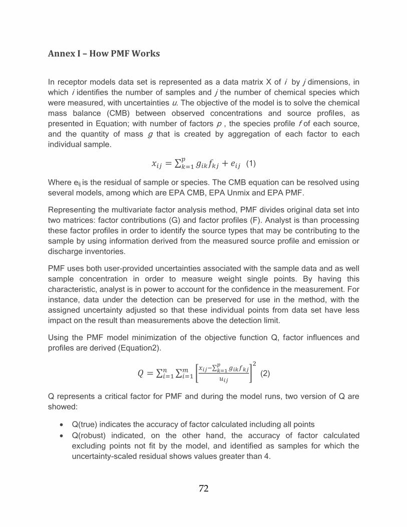
72

Annex I – How PMF Works

In receptor models data set is represented as a data matrix X of i by j dimensions, in

which i identifies the number of samples and j the number of chemical species which

were measured, with uncertainties u. The objective of the model is to solve the chemical

mass balance (CMB) between observed concentrations and source profiles, as

presented in Equation; with number of factors p , the species profile f of each source,

and the quantity of mass g that is created by aggregation of each factor to each

individual sample.

𝑥𝑖𝑗 = ∑ 𝑔𝑖𝑘𝑓𝑘𝑗 + 𝑒𝑖𝑗𝑝𝑘=1 (1)

Where eij is the residual of sample or species. The CMB equation can be resolved using

several models, among which are EPA CMB, EPA Unmix and EPA PMF.

Representing the multivariate factor analysis method, PMF divides original data set into

two matrices: factor contributions (G) and factor profiles (F). Analyst is than processing

these factor profiles in order to identify the source types that may be contributing to the

sample by using information derived from the measured source profile and emission or

discharge inventories.

PMF uses both user-provided uncertainties associated with the sample data and as well

sample concentration in order to measure weight single points. By having this

characteristic, analyst is in power to account for the confidence in the measurement. For

instance, data under the detection can be preserved for use in the method, with the

assigned uncertainty adjusted so that these individual points from data set have less

impact on the result than measurements above the detection limit.

Using the PMF model minimization of the objective function Q, factor influences and

profiles are derived (Equation2).

𝑄 = ∑ ∑ [𝑥𝑖𝑗−∑ 𝑔𝑖𝑘𝑓𝑘𝑗

𝑝𝑘=1

𝑢𝑖𝑗]2

𝑚𝑖=1

𝑛𝑖=1 (2)

Q represents a critical factor for PMF and during the model runs, two version of Q are

showed:

Q(true) indicates the accuracy of factor calculated including all points

Q(robust) indicated, on the other hand, the accuracy of factor calculated

excluding points not fit by the model, and identified as samples for which the

uncertainty-scaled residual shows values greater than 4.

73

The differentiation between Q(true) and Q(robust) create a measure of the impact of

data points which have high scaled residuals. Usually peak influences from sources that

are not present during the sampling time period are connected with these points.

However, in some cases uncertainties may be too high which implies similar Q(true) and

Q(robust) values because the residuals are scaled by the uncertainty.

PMF model requires various iterations of the Miltilinear Engine (ME) in order to support

identification of the most optimal factor influences and profiles. This is needed because

of the nature of the ME procedure that initiates the search for the consistent factor

profiles with a randomly created factor profile. Additionally, this factor profile is adjusted

by the gradient approach with an aim to graph the ideal path to the best solution. In

other words, the model creates a multidimensional space using the measurement

samples and then passes through the space using the gradient approach to arrive to its

final destination of the best result along the path. Identification of the best solution

usually implies the lowest Q(robust) value along the path (i.e. the minimum Q) and it

may be perceived as the bottom point of the through in the multidimensional space.

Since the random starting point is determined by the seed valued and the path which

dictates it, there is no assurance that the gradient approach will always identify the

lowest point in the multidimensional space (global minimum), but instead, it may find the

local minimum. In order to increase the chance of reaching the global minimum, the

model should be run at least 20 times for the development of the solution and 100 times

for the final solution, with a choice of different starting point every time.

The points that are not fit by the PMF does not influence the Q(robust), it is normally

used as a parameter for a choice of the optimal run from the various ones. Likewise, the

variability of Q(robust) gives an information if the starting run solutions have great

variability, because of the random seed which is used to initiate the gradient algorithm in

diverse positions. If the provision of the stabilized path towards the minimum is obtained

by data used, Q(robust) will have only little variations between the runs. On the other

hand, the arrangement of the starting point and the space defined by the data set will

impact the direction to the minimum value, resulting in that way in diverse values of

Q(robust). The best optimal solution is created by the lowest value of the Q(robust), and

it is used by default.

Another influence in factor profiles among PMF runs can be noted if some chemical

transformations or changes in processes appear. In order to evaluate the variations

between runs, two approaches are available: intra-run residual analysis and a factor

summary of the species distribution compared to those of the lowest Q(robust) run.

Evaluation of all the error estimates in PMF is performed by the analyst. Lastly, the

variation in the PMF results can be assessed with the following three methodologies:

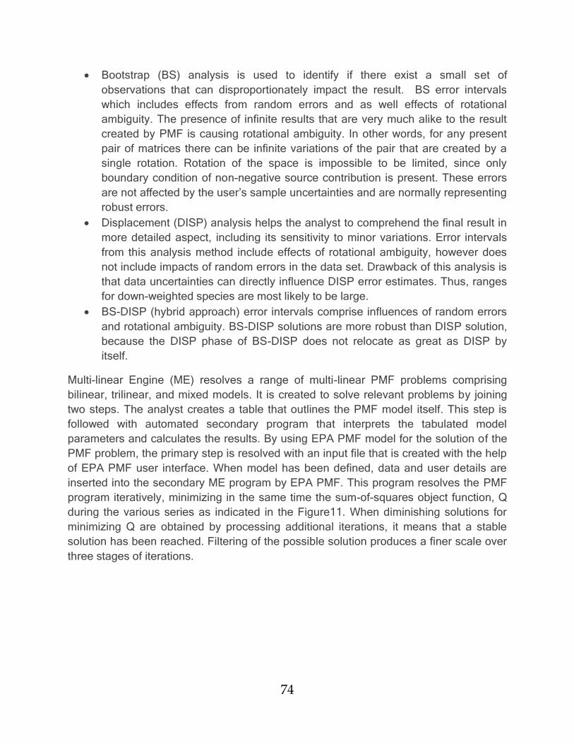
74

Bootstrap (BS) analysis is used to identify if there exist a small set of

observations that can disproportionately impact the result. BS error intervals

which includes effects from random errors and as well effects of rotational

ambiguity. The presence of infinite results that are very much alike to the result

created by PMF is causing rotational ambiguity. In other words, for any present

pair of matrices there can be infinite variations of the pair that are created by a

single rotation. Rotation of the space is impossible to be limited, since only

boundary condition of non-negative source contribution is present. These errors

are not affected by the user’s sample uncertainties and are normally representing

robust errors.

Displacement (DISP) analysis helps the analyst to comprehend the final result in

more detailed aspect, including its sensitivity to minor variations. Error intervals

from this analysis method include effects of rotational ambiguity, however does

not include impacts of random errors in the data set. Drawback of this analysis is

that data uncertainties can directly influence DISP error estimates. Thus, ranges

for down-weighted species are most likely to be large.

BS-DISP (hybrid approach) error intervals comprise influences of random errors

and rotational ambiguity. BS-DISP solutions are more robust than DISP solution,

because the DISP phase of BS-DISP does not relocate as great as DISP by

itself.

Multi-linear Engine (ME) resolves a range of multi-linear PMF problems comprising

bilinear, trilinear, and mixed models. It is created to solve relevant problems by joining

two steps. The analyst creates a table that outlines the PMF model itself. This step is

followed with automated secondary program that interprets the tabulated model

parameters and calculates the results. By using EPA PMF model for the solution of the

PMF problem, the primary step is resolved with an input file that is created with the help

of EPA PMF user interface. When model has been defined, data and user details are

inserted into the secondary ME program by EPA PMF. This program resolves the PMF

program iteratively, minimizing in the same time the sum-of-squares object function, Q

during the various series as indicated in the Figure11. When diminishing solutions for

minimizing Q are obtained by processing additional iterations, it means that a stable

solution has been reached. Filtering of the possible solution produces a finer scale over

three stages of iterations.

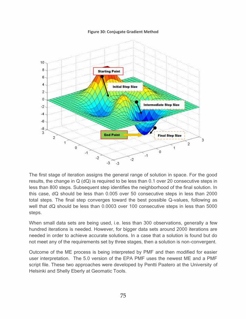
75

Figure 30: Conjugate Gradient Method

The first stage of iteration assigns the general range of solution in space. For the good

results, the change in Q (dQ) is required to be less than 0.1 over 20 consecutive steps in

less than 800 steps. Subsequent step identifies the neighborhood of the final solution. In

this case, dQ should be less than 0.005 over 50 consecutive steps in less than 2000

total steps. The final step converges toward the best possible Q-values, following as

well that dQ should be less than 0.0003 over 100 consecutive steps in less than 5000

steps.

When small data sets are being used, i.e. less than 300 observations, generally a few

hundred iterations is needed. However, for bigger data sets around 2000 iterations are

needed in order to achieve accurate solutions. In a case that a solution is found but do

not meet any of the requirements set by three stages, then a solution is non-convergent.

Outcome of the ME process is being interpreted by PMF and then modified for easier

user interpretation. The 5.0 version of the EPA PMF uses the newest ME and a PMF

script file. These two approaches were developed by Pentti Paatero at the University of

Helsinki and Shelly Eberly at Geomatic Tools.

76

The PMF model requires a data set that contains a range of parameters which have

been measured across various samples. More specifically, PM2.5 data set comprises of

10 to 20 species over 100 samples. However, an uncertainty data set is also necessary

for the complete calculation. This data set is calculated by using propagated

uncertainties or some similar accessible information, for instance collated sampling

precision.

Application of the PMF is connected to a wide range of data, including 24-hour PM2.5,

size resolved aerosol, deposition, air toxics, high time resolution measurements, i.e.

aerosol mass spectrometers (AMS) and volatile organic compound (VOC) data.