Faculty of Engineering Technology (CTW)

Sound transmission inturbomachinery flow ductsInternship at DLR-Berlin

s1005812 Peter PuttkammerJanuary 15, 2015

Guidance:U. Tapken DLR-BerlinM. Behn DLR-BerlinProf. dr. L. Enghardt DLR-BerlinProf. dr. H.W.M. Hoeijmakers University of Twente

2

Contents

Nomenclature 4

1 Introduction 7

2 Literature 92.1 Transmission and reflection of single blade rows . . . . . . . . . . . . . . . . . . 92.2 Frequency and mode scattering . . . . . . . . . . . . . . . . . . . . . . . . . . . 102.3 Mode trapping and acoustic resonance . . . . . . . . . . . . . . . . . . . . . . . 112.4 Summary . . . . . . . . . . . . . . . . . . . . . . . . . . . . . . . . . . . . . . . 12

3 Theoretical expressions for pressure modes 133.1 Pressure wave in cylindrical duct . . . . . . . . . . . . . . . . . . . . . . . . . . 133.2 Pressure wave in unwrapped cylindrical duct . . . . . . . . . . . . . . . . . . . . 143.3 Mode and frequency scattering . . . . . . . . . . . . . . . . . . . . . . . . . . . . 163.4 Inter-vane phase difference . . . . . . . . . . . . . . . . . . . . . . . . . . . . . . 173.5 Wave modes from stator . . . . . . . . . . . . . . . . . . . . . . . . . . . . . . . 203.6 Wave modes from rotor . . . . . . . . . . . . . . . . . . . . . . . . . . . . . . . . 203.7 Transmission and reflection coefficients . . . . . . . . . . . . . . . . . . . . . . . 22

4 Blade row model of Smith with mean stream flow 234.1 Principle concept . . . . . . . . . . . . . . . . . . . . . . . . . . . . . . . . . . . 244.2 Governing Equations . . . . . . . . . . . . . . . . . . . . . . . . . . . . . . . . . 244.3 Incoming pressure wave . . . . . . . . . . . . . . . . . . . . . . . . . . . . . . . . 254.4 Solution for one vortex row . . . . . . . . . . . . . . . . . . . . . . . . . . . . . 264.5 Upwash integral equation . . . . . . . . . . . . . . . . . . . . . . . . . . . . . . . 274.6 Far field acoustic waves . . . . . . . . . . . . . . . . . . . . . . . . . . . . . . . . 284.7 Numerical evaluation upwash integral equation . . . . . . . . . . . . . . . . . . . 284.8 Numerical evaluation acoustic wave amplitudes . . . . . . . . . . . . . . . . . . 31

5 Blade row model of Smith without mean stream flow 335.1 Governing equations . . . . . . . . . . . . . . . . . . . . . . . . . . . . . . . . . 335.2 Incoming pressure wave . . . . . . . . . . . . . . . . . . . . . . . . . . . . . . . . 345.3 Solution of one vortex row . . . . . . . . . . . . . . . . . . . . . . . . . . . . . . 345.4 Upwash integral equation . . . . . . . . . . . . . . . . . . . . . . . . . . . . . . . 355.5 Far field acoustic waves . . . . . . . . . . . . . . . . . . . . . . . . . . . . . . . . 365.6 Numerical evaluation upwash integral equation and acoustic wave amplitudes . . 36

6 Results 396.1 Typical results of blade row models . . . . . . . . . . . . . . . . . . . . . . . . . 396.2 Implementation in MATLAB . . . . . . . . . . . . . . . . . . . . . . . . . . . . 396.3 Raw results . . . . . . . . . . . . . . . . . . . . . . . . . . . . . . . . . . . . . . 40

3

4 CONTENTS

7 Conclusion 437.1 Main conclusions . . . . . . . . . . . . . . . . . . . . . . . . . . . . . . . . . . . 437.2 Recommendations . . . . . . . . . . . . . . . . . . . . . . . . . . . . . . . . . . . 43

Bibliography 44

A Power coefficients 47

B MATLAB scripts 49B.1 Main upstream . . . . . . . . . . . . . . . . . . . . . . . . . . . . . . . . . . . . 49B.2 Kernel whitehead . . . . . . . . . . . . . . . . . . . . . . . . . . . . . . . . . . . 52B.3 V whitehead . . . . . . . . . . . . . . . . . . . . . . . . . . . . . . . . . . . . . . 53

Nomenclature

′ Term of amplitude without dependency of vorticity

+ Upstream propagating wave

− Downstream propagating wave

αi Angle of incidence of pressure waves

αs Stagger angle

αi,Jenkins Angle of incidence of pressure waves by convention of Jenkins

αi,Kaji Angle of incidence of pressure waves by convention of Kaji and Okazaki

v Upwash velocity

¯ Reference frame with x-axis along the blade chord

β√

1−M2

ˇ Reference frame corresponding to stationary blades and moving duct

ˆ Amplitude

P Sound power

R Reflection coefficient

T Transmission coefficient

µ Axial component of the wave number

ν Gap-wise component of the wave number

Ω Angular frequency

ω0 Acoustic frequency

φ Circumferential coordinate

ρ0 Fluid density

σ Inter-vane phase difference

˜ Normalized quantities

a Speed of sound

B Number of blades

5

6 CONTENTS

c Blade chord

I Power intensity

k Wave number

M Mach number

m Circumferential wave mode order

N Total number of collocation points

n Radial wave mode order

p Pressure perturbation

r Radial coordinate / integer corresponding to scattering mechanism

R0 Distance between midpoint of blades and center of duct

s Blade gap

t Time

U Axial component of mean stream velocity

u Axial component of velocity perturbation

V Gap-wise component of mean stream velocity

v Gap-wise component of velocity perturbation

W Mean stream velocity

x Axial coordinate

y Gap-wise coordinate

Chapter 1

Introduction

The main objective of turbomachines is to transfer energy between the rotating impeller bladesand the working fluid, in the form of increased/decreased fluid velocity and/or pressure. Asa consequence of the change in pressure, pressure waves are formed. These waves propagatethrough turbomachines, are transmitted and reflected by blade rows and are radiated to the’far-field’ where one experience these waves as noise. The sound intensity radiated from the ductopening may considered to be influenced by the transmission and reflection of the blade rows.Therefore, besides generation of sound, blade rows play an important role in the propagationof sound waves through a turbomachine.

This research is carried out as part of a project (T2.1 Transmission and Reflection of BladeRows) of the German Aerospace Center (Deutsches Zentrum fur Luft- und Raumfahrt, DLR).The main objectives for this project are:

Accurate modeling of the propagation of sound through turbomachine stages using ana-lytical methods.

Development of guidelines for optimizing blade geometries in order to reduce sound trans-mission through blade row.

The objective of present study is to carry out a literature review with regard to existinganalytical models that describe the propagation of sound waves through turbomachinery bladerows. From this literature study, an appropriate model is selected for implementation. Theidea is to rewrite the blade row model of Smith [1] such that it can be applied for sound wavespropagating through a stator without mean stream flow. It will be seen that the theoreticalmodel is obtained, however the implementation into a calculation program (in this reportMATLAB is used) is not (yet) complete.

The literature review regarding existing blade row models is the subject of chapter 2. Thegeneral theory for duct acoustics regarding rotors and stators in circular ducts is found inchapter 3. Chapters 4 and 5 discuss the analytical model of Smith. First the original modelof Smith - with mean stream flow - is presented, followed by the reformulated model whichcan be applied for cases without mean stream flow. The first raw results - which are not yetsatisfactory - are presented in chapter 6. Finally a conclusion and recommendations are drawnin chapters 7.

7

8 CHAPTER 1. INTRODUCTION

Chapter 2

Literature

The present study examines different models for determining the transmission and reflection ofsound waves through blade rows. This topic has been subject of multiple studies for the last40 years, where many developments are achieved. In this section a different blade row modelsare discussed.

Transmission and reflection of blade rows is first modeled in the beginning of the 1970’s. Inthis period it is identified that the transmission and reflection of pressure waves depend on theincident wave mode. Furthermore concepts such as frequency and mode scattering, althoughnot explicitly mentioned, can be incorporated in the models of the 1970’s. From the end of1990’s the computation of a stage (rotor + stator) is investigated, using numerical schemesfor coupling different blade rows. Due to the ability of modeling multiple blade rows, otherphenomena became of interest such as mode trapping and acoustic resonance. It should benoted that there can be more blade row models found in literature. The selection made in thisstudy is based on the fact that the models specifically discuss the transmission and reflectionproperties.

2.1 Transmission and reflection of single blade rows

In order to determine the transmission and reflection of sound waves through blade rows, dif-ferent approaches are investigated by different authors for finding the solution of the equationsof compressible flow through a blade row. The methods used vary widely regarding the choiceof blade row models and mathematical techniques.

The different models discussed below share a couple of significant assumptions. All bladerow models are two-dimensional, but for the blade row model of Glegg [2]. Even Muir [3], whodiscusses the incidence of three-dimensional waves, uses a two-dimensional semi-actuator disk.Effects of viscosity are neglected and the flow is assumed isentropic. The incoming acousticwaves are plane harmonic waves. Furthermore the blades are unloaded, but Kaji and Okazaki [4]have shown that the effect of blade loading for most incidence angles has little significance.

Kaji and Okazaki (1970) [5] introduced a so-called ’semi-actuator disk’ which divided theflow field in three regions: upstream, downstream and within the blades. The semi-actuatordisk is a blade row of two-dimensional, flat plates of zero thickness and finite length. However,the blade gap (distance between leading edges of neighboring blades) is infinitesimally small. Inthis paper only one transmitted and reflected wave are considered. Matching the mass-flux andthe pressure at the leading and trailing edges leads to transmission- and reflection coefficients.Muir (1977) [3] generalizes, using an average frequency approach, the semi-actuator disk modelto include the incidence of three-dimensional sound waves.

Another possibility for representing a blade row is cascade modeling. In the second part oftheir paper, Kaji and Okazaki (1970) [4] adopted an approach to incorporate a blade row where

9

10 CHAPTER 2. LITERATURE

the blade gap is of finite distance. In this approach each blade is represented by an unsteadydistribution of pressure doublets which is induced by the incident acoustic pressure wave. Incombination with the condition of zero net upwash (normal velocity component) at the bladesurface, an integral equation for the unknown doublet distribution function is derived. Thesolution of the integral equation - which relates the source strength to the velocity and pressuredisturbance - is obtained using a collocation procedure, from which the transmitted and reflectednoise is determined. Smith (1973) [1] used, instead of pressure doublets, vortices to representthe blades. By doing so, an integral equation for the unknown vorticity distribution along thecascade blades is obtained again using the collocation technique. The change from pressuredoublets to vorticity sources is done since it leads to considerable mathematical simplifications.

Mani and Horvay (1970) [6] obtained solutions for the transmission and reflection of bladerows using an approximate solution based on the Wiener-Hopf technique. This technique is usedto couple solutions of two partial differential equations with mixed boundary conditions at thesame boundary. Mani and Horvay identified two different problems, an incidence and emissionproblem. The incidence problem covers a plane wave impinging on an infinite set of semi-infiniteblades, the emission problem deals with the radiation of the excited blade channel modes bythe incident wave at the open ends of a row of semi-infinite blades. These two solutions arecombined using the mentioned Wiener-Hopf technique, from which estimates of the transmissionand reflection properties of the blade row are derived. Koch (1971) [7] developed the work ofMani and Horvay for blades with finite chord. Koch derives a solution for the reflected andtransmitted sound for both upstream and downstream propagating acoustic waves.

Amiet (1971) [8] uses classical isolated flat-plate airfoil theory and the linearized Eulerequations to calculate the transmission and reflection of a blade row. In order to do so, Amietseparates the problem into a near- and far-field problem, from which a closed formulation of theproblem is stated. Although theoretically this approach can be understood well, the practicalimplementation seemed rather difficult since it deals with isolated blades rather than a bladerow. Therefore this theory it is not used in many blade row models developed after the 1970’sin contrast to the models of Kaji and Okazaki, Smith and Koch.

Important parameters that influence the transmission and reflection of sound waves throughblade rows is investigated by Kaji and Okazaki [4], and confirmed by others (e.g. [7], [8]). Theflow Mach number and the angle of incidence both have great influence on the transmission.For increasing Mach numbers, the transmission coefficient will decrease. Furthermore soundwaves hitting the blade row at large angle of incidence can resemble a sound wave hitting awall, which of course will decrease the transmission coefficient. Kaji and Okazaki also foundthat the wave length and the steady aerodynamic blade loading both have minor influence onthe transmission coefficient.

2.2 Frequency and mode scattering

Although not explicitly mentioned, frequency and mode scattering is incorporated in the bladerow models of Kaji and Okazaki [4], Smith [1] and Koch [7]. Furthermore Kaji and Okazakirecognized that the transmission and reflection is influenced by the incoming wave mode. Theydefined two conditions, a sub- and super-resonant condition. In the sub-resonant conditionthe transmitted and reflected wave have the same wavelengths as the incoming wave, implyingfrequency and mode scattering will not occur. For the super-resonant condition also waveswith wavelengths different from the incoming wave starts to propagate in up- and downstreamdirection due to the fact that the waves can be scattered in terms of frequency and mode. Kochand Smith discuss and implement these definitions in their respective papers.

Topol (1987) [9] concretized the transmitted and reflected waves for the super-resonant

2.3. MODE TRAPPING AND ACOUSTIC RESONANCE 11

condition. To come to this concretization, Topol introduces a model containing one rotorand stator blade row (called a ’stage’), for which a rather simple analytical model is derivedwhich shows that noise modes at blade passing frequency (BPF) can be ’cut-off’ (decayingwave modes) in the in- and outlet of the turbomachine, but can be ’cut-on’ (propagating wavemodes) in the region between the rotor and the stator (’swirl region’). This indicates that BPFmode noise impinging to the stator is partly reflected and propagating upstream towards therotating rotor blades. Incidence with the rotor blades induces noise which is reflected from therotor containing partially carried in modes at higher harmonics of BPF that are also cut-on.It is shown that these modes with higher harmonics can dominate the overall noise at specificrotor angular velocities. Comparisons with model fan test, conducted and described in thispaper, and full-scale engine data are carried out.

This frequency scattering by rotating rotor blades, described by Topol, is not the only scattermechanism that needs to be considered. Also modal scattering is an important feature, sinceit not only takes place at the rotating rotor, but also at the stationary stator. In cylindricalducts the circumferential mode orders are restricted to the values of m (m = nB − kV ) [10]resulting from integer values of the rotor n and stator scattering indices k. B is the number ofrotor blades, V is the number of stator vanes. Hanson (1993) [11] formulated a model, basedon the method of Smith, which includes this mode scattering mechanism for a coupled systemof a rotor, a stator and the in- and outlet of a turbomachine. It is stated that the rotor willscatter on the index n, and the stator will scatter on the index k. In 1997 Hanson [12] wrotesa second paper, where the fundamental behavior of the scattering coefficients is examined fora better understanding of the role of blade row transmission and reflection in noise generation.It is shown that the vane/blade ratio significantly influences the transmission and reflection ofdifferent wave modes. Furthermore it is shown that rotors tend to scatter up in BPF orderwhere the reflected energy can exceed the incident energy by a substantial amount.

Above mentioned models of Topol and Hanson are valid for tonal noise. However, they donot describe the transmission and reflection of broadband noise. Hanson (2001) [13] adoptedthe rectilinear cascade model of Glegg (1999) [2] and developed a coupled model for broadbandnoise. Glegg derived exact analytical expressions for the acoustic field radiated from a three-dimensional blade row, in contrast to the two-dimensional model of Smith. Hanson discoveredan analytical approach for tracking broadband noise modes dividing them into what he calls’independent mode sub-sets’. This makes the broadband problem tractable and it is the basisfor the analysis.

Also based on Glegg, Posson (2013) [14] discusses a model for a ”study that aims to developand assess an analytical model for the sound transmission through an annular stator row in aconfiguration without mean flow”. In this study, Glegg’s rectilinear model for a single blade rowis used to calculate the transmission and reflection of pressure waves (see Posson, Appendix A).Posson extends this model to an annular stator row, from which satisfactory results are found.One should however be aware that the mathematical background of this advanced model iscomplex, which can make it difficult to understand the physics and the usability of this model.

2.3 Mode trapping and acoustic resonance

Another important contribution of Hanson [11] is the formulation of a generalized couplingscheme, for which isolated elements such as the stator and the rotor can be calculated as onesystem. When the system is modeled with coupling and swirl included, a phenomenon Hansoncalls ’mode trapping’ is identified. When a wave mode is trapped between a rotor and stator rowit can build up to high levels as it couples to the higher harmonics. These higher harmonics canescape to the in- or outlet, for which it is explained that the noise escaping from the system is at

12 CHAPTER 2. LITERATURE

higher harmonics. So at specific rotor rotating speeds, where mode trapping occurs, the higherharmonics can dominate the overall noise. Topol (1997) [15], employing the additional theoryof Hanson, presents an alternative method for a coupled system from which similar results arefound. Silkowski (1997) [16] - awarded the Best Paper Award 1997 from the Structures andDynamics Committee - also derives a coupled mode analysis, extended for blades with camberand thickness.

Additional contribution to the overall noise level that is recently investigated is the topicof acoustic resonance. When traveling pressure waves constructively interfere with each otherone speaks of acoustic resonance. This phenomenon can take place between a rotor and statorat specific conditions, which results in a (dominating) contribution to the overall noise levels.Pioneering work on acoustic resonance is studied by Parker and co-workers (e.g. [17]). Hellmich(2008) [18] investigates acoustic resonance in a high-speed axial compressor, using the bladerow model of Koch. Hellmich states that acoustic resonance is excited at high rotor speedswith comparably low mass flow only.

2.4 Summary

The blade row models of Smith and Koch are widely used in literature.

Frequency scattering occurs only at rotors. Mode scattering occurs at both rotors andstators.

Coupled numeric schemes are used to carry out calculations on stages instead of isolatedblade rows.

Mode trapping and acoustic resonance should be considered for calculations on coupledblade rows.

Chapter 3

Theoretical expressions for pressuremodes

Industrial turbomachines and airplane engines generate sound which radiates through, mostlycircular, ducts. These ducts restrict the sound propagation characteristics by correspondingboundary conditions. The study of the propagation of sound waves through ducts is called’Duct Acoustics’ [19]. The equations in this chapter are valid for flows with and without meanflow. If there is mean flow present, it is assumed that this mean stream flow passes throughthe cascade undeflected.

3.1 Pressure wave in cylindrical duct

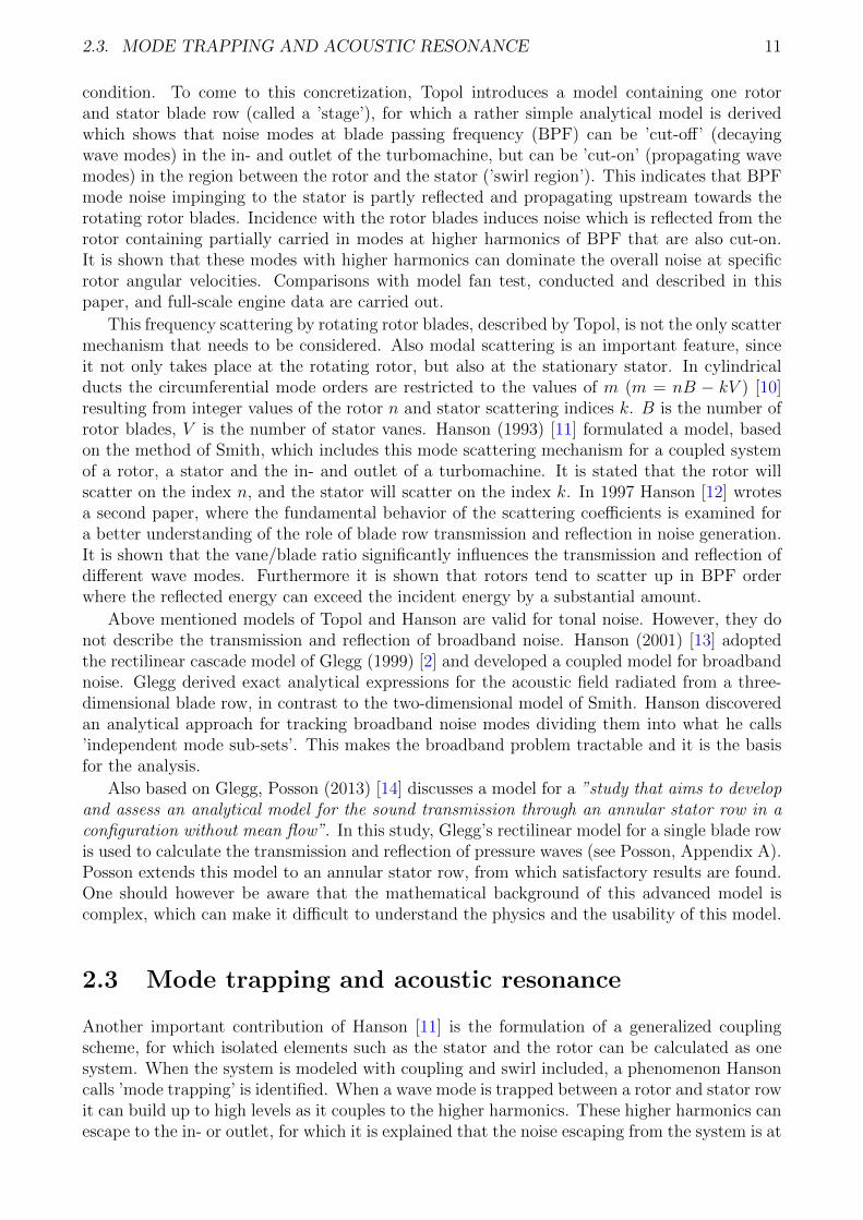
The governing equations supporting the theory of duct acoustics are based on the conservationequations of mass, momentum and energy. The propagation of sound - for ducts with variouscross-sections and different conditions of flow - has been subject of many studies. By assumingthat acoustic fluctuations are small perturbations of pressure, density, velocity and temperature,the linearized conservation equations can be derived. Combining these linearized equationsleads to the derivation of the governing wave equations, describing the propagation of soundthrough a specific duct.

Figure 3.1: cylindrical duct [19]

The wave equation can be solved using the method of separation of variables, where it isassumed that the pressure p is a function of three space coordinates (r, φ, z) and time (t). Byapplying the boundary conditions, the specific representation of the pressure wave through theduct is found. Without applying the boundary conditions, the general solution for the incoming

13

14 CHAPTER 3. THEORETICAL EXPRESSIONS FOR PRESSURE MODES

sound in terms of the pressure reads [19]:

p±n,m(x, r, φ, t) = pn,mfn,m(r)ei(ω0t+µ±n,mx+mφ) (3.1)

Where p±n,m is a pressure wave mode, depending on the spatial and time coordinates and theradial and circumferential wave mode order. Furthermore pn,m is the amplitude of the wavemode, f(r) a function - typically expressible in terms of Bessel functions - depending on theradial position r, the acoustic frequency ω0 and the axial and circumferential wave numbers µ±mand m. The ± sign indicates the direction of propagation, ’+’ is a pressure wave propagatingupstream, ’−’ a wave in downstream direction. One should be aware that this ’plus-minus’ signconvention can be used different in literature.

3.2 Pressure wave in unwrapped cylindrical duct

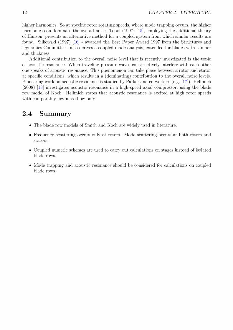
In order to investigate the transmission and reflection characteristics of a blade row, a two-dimensional model is often used in literature. Therefore the three-dimensional wave mode(equation 3.1) should be converted into a two-dimensional wave mode and similar considerationsare needed for the blade row.

The cascade model is used to represent the circular blade row. It is necessary to adoptsimplifying assumptions since rotor blades and stator vanes have complex geometry (thickness,shape changes, camber, angles). A rotor/stator is divided in so-called annular strips. Thesestrips are unwrapped to form a two-dimensional blade row (’cascade’) consisting of flat plateswith zero thickness. In figure 3.2 this procedure is displayed.

Figure 3.2: Unwrapped cascade model [20]

The incoming sound should be rewritten in terms of this unwrapped cascade model. Inorder to carry out this procedure, the radial dependency is neglected. This can be assumedsince the radial variation of the pressure waves is small compared to the circumferential andaxial variation. Topol [15] showed that the influence of radial modes is only significant whenrotor/stator interaction is considered at high rotor speeds including mode scattering. So forrelations of single rotors or stators this radial dependency can be neglected. A linear coordinatetransformation of the circumferential coordinate φ is applied by writing it as the gap-wisecoordinate divided by the distance between the midpoint of the blades and the center of thecircular duct R0 (see figure 3.3):

φ =y

R0

(3.2)

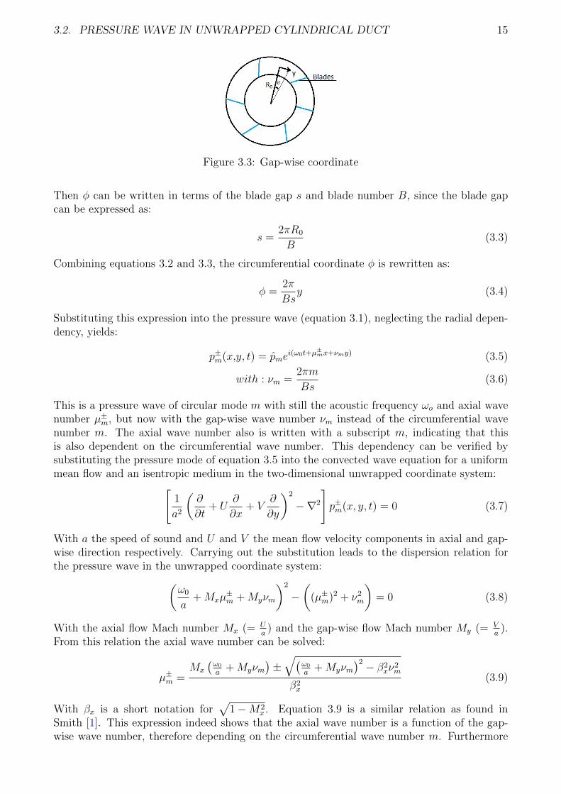
3.2. PRESSURE WAVE IN UNWRAPPED CYLINDRICAL DUCT 15

Figure 3.3: Gap-wise coordinate

Then φ can be written in terms of the blade gap s and blade number B, since the blade gapcan be expressed as:

s =2πR0

B(3.3)

Combining equations 3.2 and 3.3, the circumferential coordinate φ is rewritten as:

φ =2π

Bsy (3.4)

Substituting this expression into the pressure wave (equation 3.1), neglecting the radial depen-dency, yields:

p±m(x,y, t) = pmei(ω0t+µ

±mx+νmy) (3.5)

with : νm =2πm

Bs(3.6)

This is a pressure wave of circular mode m with still the acoustic frequency ωo and axial wavenumber µ±m, but now with the gap-wise wave number νm instead of the circumferential wavenumber m. The axial wave number also is written with a subscript m, indicating that thisis also dependent on the circumferential wave number. This dependency can be verified bysubstituting the pressure mode of equation 3.5 into the convected wave equation for a uniformmean flow and an isentropic medium in the two-dimensional unwrapped coordinate system:[

1

a2

(∂

∂t+ U

∂

∂x+ V

∂

∂y

)2

−∇2

]p±m(x, y, t) = 0 (3.7)

With a the speed of sound and U and V the mean flow velocity components in axial and gap-wise direction respectively. Carrying out the substitution leads to the dispersion relation forthe pressure wave in the unwrapped coordinate system:(

ω0

a+Mxµ

±m +Myνm

)2

−(

(µ±m)2 + ν2m

)= 0 (3.8)

With the axial flow Mach number Mx (= Ua

) and the gap-wise flow Mach number My (= Va

).From this relation the axial wave number can be solved:

µ±m =Mx

(ω0

a+Myνm

)±√(

ω0

a+Myνm

)2 − β2xν

2m

β2x

(3.9)

With βx is a short notation for√

1−M2x . Equation 3.9 is a similar relation as found in

Smith [1]. This expression indeed shows that the axial wave number is a function of the gap-wise wave number, therefore depending on the circumferential wave number m. Furthermore

16 CHAPTER 3. THEORETICAL EXPRESSIONS FOR PRESSURE MODES

this indicates the difference between the so-called ’cut-on’ and ’cut-off’ wave modes. If µ±m isreal valued, the wave mode is cut-on, which indicates that the pressure waves will propagateup- and downstream. If µ±m has an imaginary part, the wave modes will decay exponentiallyand therefore not propagate towards the up- and downstream infinity (cut-off). So the wavemode is cut-on if: (ω0

a+Myνm

)2

− β2xν

2m > 0 (3.10)

Summarizing the notation for an incoming pressure wave, created by sound of acoustic fre-quency ω0 far up- (-) or downstream (+), applied in the unwrapped two-dimensional referenceframe with amplitude pinc,m (subscript ’inc’ denotes the incoming pressure wave), the axialcomponent x and the gap-wise component y, of circumferential mode order m impinging ablade row of B blades and blade gap s:

p±inc,m(x, y, t) = pinc,mei(ω0t+µ

±inc,mx+νinc,my)

with : νinc,m =2πm

Bs

and : µ±inc,m =Mx

(ω0

a+Myνinc,m

)±√(

ω0

a+Myνinc,m

)2 − β2xν

2inc,m

β2x

(3.11)

3.3 Mode and frequency scattering

Already discussed in the literature chapter, mode and frequency scattering are phenomenaoccurring with sound waves impinging on rotors and stators. Mode scattering is the mechanismof an incident wave consisting of a single circumferential wave mode m which is reflected andtransmitted in pressure waves consisting of multiple wave modes due to the periodic natureof the blade rows. When the blade rows also move (rotors), the frequency of the transmittedand reflected can be shifted into other frequencies, which is called frequency scattering. It willbe shown that the scattered modes and frequencies are not random but behave such that thismechanism can be analyzed.

Also discussed in the literature chapter are the sub- and super-resonant conditions. Theseconditions are first described in the paper of Kaji and Okazaki [4] and they indicate whetheror not scattering will occur. In their paper explicit relations are formulated and it can beunderstood by this simple example. If the gap-wise component of the wavelength is smallenough such that at least a half period wave impinges between the leading edges of two blades,the condition is called super-resonant and frequency and mode scattering will occur. If halfa period does not fit between the blades, the wavelength is too long compared to the bladegap, the condition is called sub-resonant, and therefore no scattering will occur. Since in thisreport only the sub-critical regime is investigated, the sub-critical condition is presented. Thecondition is sub-resonant if the wave number, which is a combination of the axial and gap-wisewave number (k2 = µ2 + ν2), satisfies:

k ≤ π

s

1−M2

√1−M2 cos2 αs

(3.12)

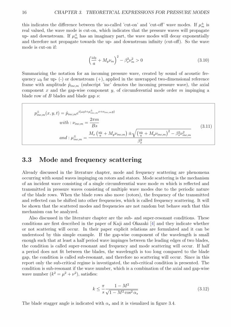
The blade stagger angle is indicated with αs and it is visualized in figure 3.4.

3.4. INTER-VANE PHASE DIFFERENCE 17

3.4 Inter-vane phase difference

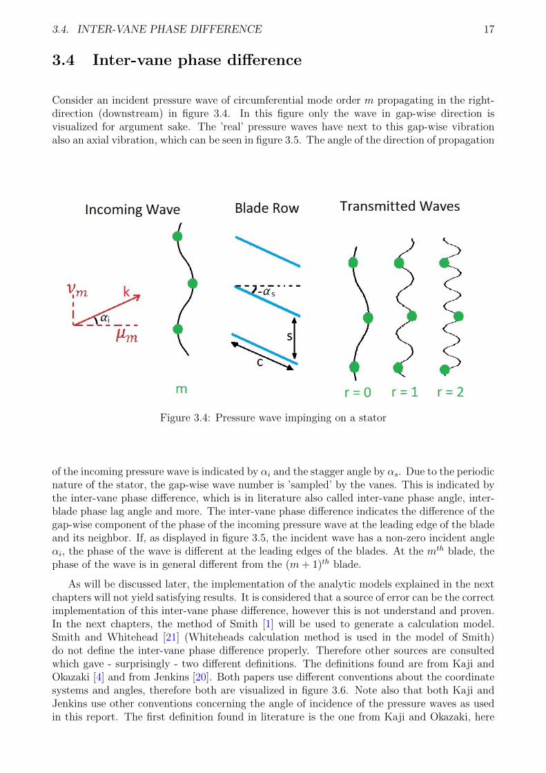
Consider an incident pressure wave of circumferential mode order m propagating in the right-direction (downstream) in figure 3.4. In this figure only the wave in gap-wise direction isvisualized for argument sake. The ’real’ pressure waves have next to this gap-wise vibrationalso an axial vibration, which can be seen in figure 3.5. The angle of the direction of propagation

Figure 3.4: Pressure wave impinging on a stator

of the incoming pressure wave is indicated by αi and the stagger angle by αs. Due to the periodicnature of the stator, the gap-wise wave number is ’sampled’ by the vanes. This is indicated bythe inter-vane phase difference, which is in literature also called inter-vane phase angle, inter-blade phase lag angle and more. The inter-vane phase difference indicates the difference of thegap-wise component of the phase of the incoming pressure wave at the leading edge of the bladeand its neighbor. If, as displayed in figure 3.5, the incident wave has a non-zero incident angleαi, the phase of the wave is different at the leading edges of the blades. At the mth blade, thephase of the wave is in general different from the (m+ 1)th blade.

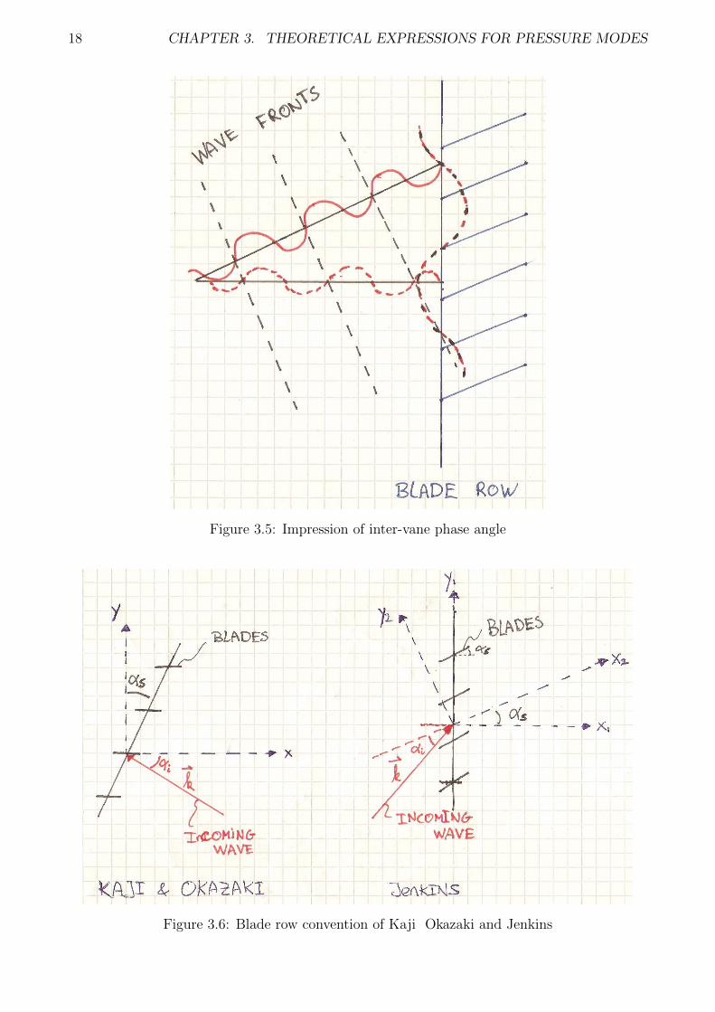
As will be discussed later, the implementation of the analytic models explained in the nextchapters will not yield satisfying results. It is considered that a source of error can be the correctimplementation of this inter-vane phase difference, however this is not understand and proven.In the next chapters, the method of Smith [1] will be used to generate a calculation model.Smith and Whitehead [21] (Whiteheads calculation method is used in the model of Smith)do not define the inter-vane phase difference properly. Therefore other sources are consultedwhich gave - surprisingly - two different definitions. The definitions found are from Kaji andOkazaki [4] and from Jenkins [20]. Both papers use different conventions about the coordinatesystems and angles, therefore both are visualized in figure 3.6. Note also that both Kaji andJenkins use other conventions concerning the angle of incidence of the pressure waves as usedin this report. The first definition found in literature is the one from Kaji and Okazaki, here

18 CHAPTER 3. THEORETICAL EXPRESSIONS FOR PRESSURE MODES

Figure 3.5: Impression of inter-vane phase angle

Figure 3.6: Blade row convention of Kaji Okazaki and Jenkins

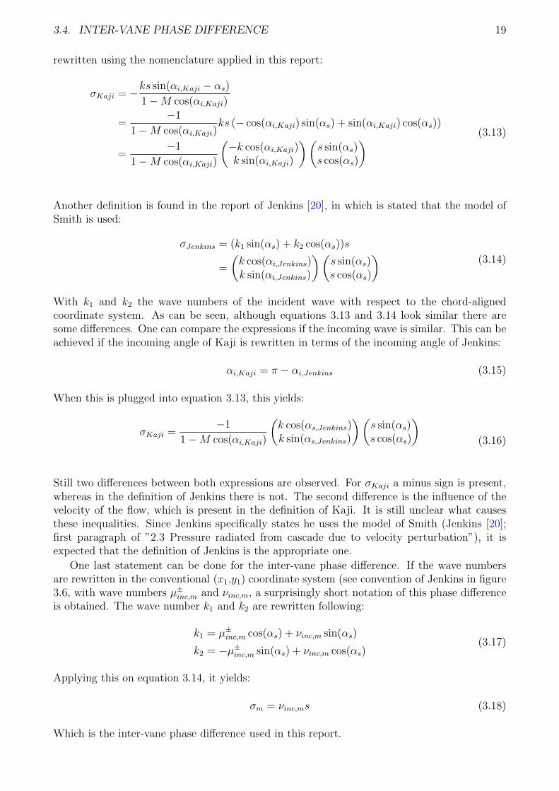
3.4. INTER-VANE PHASE DIFFERENCE 19

rewritten using the nomenclature applied in this report:

σKaji = −ks sin(αi,Kaji − αs)1−M cos(αi,Kaji)

=−1

1−M cos(αi,Kaji)ks (− cos(αi,Kaji) sin(αs) + sin(αi,Kaji) cos(αs))

=−1

1−M cos(αi,Kaji)

(−k cos(αi,Kaji)k sin(αi,Kaji)

)(s sin(αs)s cos(αs)

) (3.13)

Another definition is found in the report of Jenkins [20], in which is stated that the model ofSmith is used:

σJenkins = (k1 sin(αs) + k2 cos(αs))s

=

(k cos(αi,Jenkins)k sin(αi,Jenkins)

)(s sin(αs)s cos(αs)

)(3.14)

With k1 and k2 the wave numbers of the incident wave with respect to the chord-alignedcoordinate system. As can be seen, although equations 3.13 and 3.14 look similar there aresome differences. One can compare the expressions if the incoming wave is similar. This can beachieved if the incoming angle of Kaji is rewritten in terms of the incoming angle of Jenkins:

αi,Kaji = π − αi,Jenkins (3.15)

When this is plugged into equation 3.13, this yields:

σKaji =−1

1−M cos(αi,Kaji)

(k cos(αs,Jenkins)k sin(αs,Jenkins)

)(s sin(αs)s cos(αs)

)(3.16)

Still two differences between both expressions are observed. For σKaji a minus sign is present,whereas in the definition of Jenkins there is not. The second difference is the influence of thevelocity of the flow, which is present in the definition of Kaji. It is still unclear what causesthese inequalities. Since Jenkins specifically states he uses the model of Smith (Jenkins [20];first paragraph of ”2.3 Pressure radiated from cascade due to velocity perturbation”), it isexpected that the definition of Jenkins is the appropriate one.

One last statement can be done for the inter-vane phase difference. If the wave numbersare rewritten in the conventional (x1,y1) coordinate system (see convention of Jenkins in figure3.6, with wave numbers µ±inc,m and νinc,m, a surprisingly short notation of this phase differenceis obtained. The wave number k1 and k2 are rewritten following:

k1 = µ±inc,m cos(αs) + νinc,m sin(αs)

k2 = −µ±inc,m sin(αs) + νinc,m cos(αs)(3.17)

Applying this on equation 3.14, it yields:

σm = νinc,ms (3.18)

Which is the inter-vane phase difference used in this report.

20 CHAPTER 3. THEORETICAL EXPRESSIONS FOR PRESSURE MODES

3.5 Wave modes from stator

The gap-wise wave number of the transmitted (and reflected) sound waves is the summationof the experienced gap-wise wave number (σm/s) and the gap-wise wave numbers of waves ofthe same phase difference:

νm,r =σm + 2πr

s(3.19)

With r is a list of integers (..,−1, 0, 1, 2, ..). Applying the definition of the inter-vane phasedifference and the gap-wise component of the wave number of the incoming sound wave, thisyields:

νm,r =2π

Bs(m+ rB) =

2πj

Bs= νj (3.20)

Comparison with equation 3.6 shows that the modal order of j is given by the following scat-tering rule: j = m+ rB. Using the dispersion relation (equation 3.9), the corresponding axialwave number for the transmitted and reflected waves by a stator are found. It should be notedthat also the strength of the pressure is influenced by the blade row. Or stated differently,the amplitude is altered by the blade row. This influence is investigated and discussed usingthe method of Smith in the next chapter. Here the transmitted and reflected amplitudes aredenoted by p±m, where ’+’ still indicates an upstream propagating pressure wave (in this reportthe reflected wave) and ’-’ a downstream propagating pressure wave (respectively the transmit-ted wave). Summarizing the transmitted and reflected pressure wave modes by a stator andthe axial and gap-wise wave numbers:

p±m,r(x, y, t) = p±mei(ω0t+µ

±m,rx+νm,ry)

with : νm,r =σm + 2πr

sand : σm = νinc,ms

and : µ±m,r =Mx

(ω0

a+Myνm,r

)±√(

ω0

a+Myνm,r

)2 − β2xν

2m,r

β2x

(3.21)

3.6 Wave modes from rotor

Consider a case where the rotor blades rotate in the negative φ-direction with angular velocityΩ. In the unwrapped two-dimensional situation, the rotor moves in the negative y-directionwith velocity R0Ω. When moving blades are considered, it is convenient to work with tworeference frames. One reference frame (x, y) where the blades are moving and the duct isstationary, and one (x,y) with stationary blades and a moving duct. The reference frames arecoupled by:

x = x

y = y + ΩBs

2πt

(3.22)

The mean velocities are coupled by:

U = U

V = V + ΩBs

2π

(3.23)

3.6. WAVE MODES FROM ROTOR 21

The incident pressure wave of mode m in the fixed-duct reference frame (x, y) is given byequation 3.5. Using the relations between the different reference frames, this incoming wavecan be expressed in the fixed-blade reference frame (x, y):

p±m(x, y, t) = pinc,mei(ω0t+µ

±inc,mx+νinc,m(y−ΩBs

2πt)

= pinc,mei((ω0−mΩ)t+µ±inc,mx+νinc,my)

(3.24)

So by shifting between the reference frames, the pressure wave mode is perceived containing afrequency shift:

ωm = ω0 −mΩ (3.25)

In this reference frame with stationary blades, mode scattering can be analyzed similar as forthe stator (equation 3.19). When the gap-wise wave number for the transmitted and reflectedwaves from the rotor are found, the axial wave number can be calculated using the dispersionrelation (equation 3.9):

µ±m,r(ωm) =Mx(

ωma

+ Myνm,r)±√

(ωma

+ Myνm,r)2 − β2xνm,r

βx(3.26)

It can be shown that the axial wave number is not influenced by the motion of the blade rows.It is known that Mx = Mx, My = My + ΩBs

2πa= My + Ωm

νinc,maand βx = βx. The only term that

can contribute to a different axial wave number is:

ωma

+ Myνinc,m (3.27)

Rewriting this term yields:

ωma

+ Myνinc,m =ωma

+Myνm,r +Ωm

a(3.28)

=ωm +mΩ

a+Myνinc,m (3.29)

=ω0

a+Myνinc,m (3.30)

Which is similar as in the dispersion relation for a stationary duct (equation 3.9). Theseequalities lead to the observation that the axial wave numbers in the two reference frames areequal:

µ±m,r(ωm) = µ±m,r(ω0) (3.31)

So the transmitted and reflected pressure wave modes from a rotor (including change of ampli-tude: p±). can be written as:

p±m,r(x, y, t) = p±mei(ωmt+µ

±m,rx+νm,r y) (3.32)

These scattered wave modes can also be written back into the reference frame of the stationaryduct using equation 3.22. This procedure yields:

p±m,r(x, y, t) = p±mei(ωmt+µ

±m,rx+νm,r(y+ΩBs

2πt) (3.33)

= p±mei((ωm+(σm+2πr) ΩB

2π)t+µ±m,rx+νm,ry) (3.34)

22 CHAPTER 3. THEORETICAL EXPRESSIONS FOR PRESSURE MODES

In order to understand what is indicated with this transmitted and reflected pressure wavemodes, the definition of the inter-vane phase difference is plugged in: σm = νinc,ms. Then thefrequency term in equation 3.34 can be written as:

ωm + (σm + 2πr)ΩB

2π= ωm + (νinc,ms+ 2πr)

ΩB

2π(3.35)

Using equation 3.6, the right hand side can be rewritten into:

ωm + (2πm

Bss+ 2πr)

ΩB

2π= ωm + (m+ rB)Ω (3.36)

Now substituting the shifted frequency from equation 3.25, which yields:

ω0 −mΩ + (m+ rB)Ω = ω0 + rBΩ (3.37)

So it is observed that the frequency of the transmitted and reflected waves shift in multiplesof the blade passing frequency (BΩ) and therefore moving blades can induce both mode andfrequency scattering. The pressure wave mode and the wave numbers for the reflected andtransmitted waves from a rotor are summarized below:

p±m,r(x, y, t) = p±mei((ω0+rBΩ)t+µ±m,rx+νm,ry)

with : νm,r =σm + 2πr

s

and : µ±m,r =Mx

(ω0

a+Myνm,r

)±√(

ω0

a+Myνm,r

)2 − β2xν

2m,r

β2x

(3.38)

3.7 Transmission and reflection coefficients

In literature transmission and reflection of sound for ducts with stators and rotors is calculatedin terms of transmission and reflection coefficients. However one should be aware that thesecoefficients are not uniquely defined. One definition is the ratio of the pressure amplitudes ofthe transmitted or reflected wave and the incoming wave, for example used in Smith [1]. Sincethe pressure amplitudes can be complex valued, the transmission and reflection coefficients aredefined as:

Tm,r =

∣∣p−m,r∣∣pm,inc

Rm,r =

∣∣p+m,r

∣∣pm,inc

(3.39)

Note that it is here assumed that the incoming pressure wave is propagating in downstream (-)direction. Since the method of Smith will be applied in the next chapters, this definition of thetransmission and reflection coefficients is used in this report. However, when carrying out moreresearch on different blade row models, the other common used definition of the transmissionand reflection coefficients can be applied to examine the validity of these blade row models.This other definition is based on the ratio of the acoustic powers of the transmitted, reflectedand incoming sound waves, for example used in Hanson [11], [12]. Since it is known that theenergy is a conserved quantity, this definition of the transmission coefficient can give moreinsight on the model. This was also the idea for this report, however - as will be seen in thenext chapters - the calculation models are not yet operational. In Appendix A the transmissionand reflection coefficients based on the power ratios for situations without mean stream flow ispresented, which can be used in future research.

Chapter 4

Blade row model of Smith with meanstream flow

In this chapter the blade row model of Smith [1] is discussed. The selection for this specificmodel is based on a couple of arguments. First the model of Smith is supposed to be understoodwell and a theoretical modification of the model (as carried out in the next chapter) which isvalid for cases without mean stream flows seems feasible. Second the model of Hanson [11], [12]yields interesting results regarding the transmission of sound waves through multiple bladerows, in which Hanson applies the blade row model of Smith. Third the model of Koch isused by other departments of DLR. Therefore it is from a scientific perspective interesting toinvestigate the model of Smith to examine the similarities and differences between both models.

As indicated in the introduction, the idea is to formulate a model for acoustic waves in acircular duct impinging on a stator without mean stream flow. The blade row model of Smithhowever is only applicable for cases with mean stream flow. Therefore in the next chapter, themodel of Smith is rewritten for cases without mean stream flow. It will be showed that themodification of the model changes the governing equations and that it is not possible to setthe Mach number simply to zero in the original model of Smith. In this chapter the blade rowmodel of Smith is explained, using references to the original paper of Smith. When it is referedto an equation of Smith, it is written as ”equation (S’number’)”. It should also be noted thatthe equations from the paper of Smith are here written with the nomenclature used in thisreport.

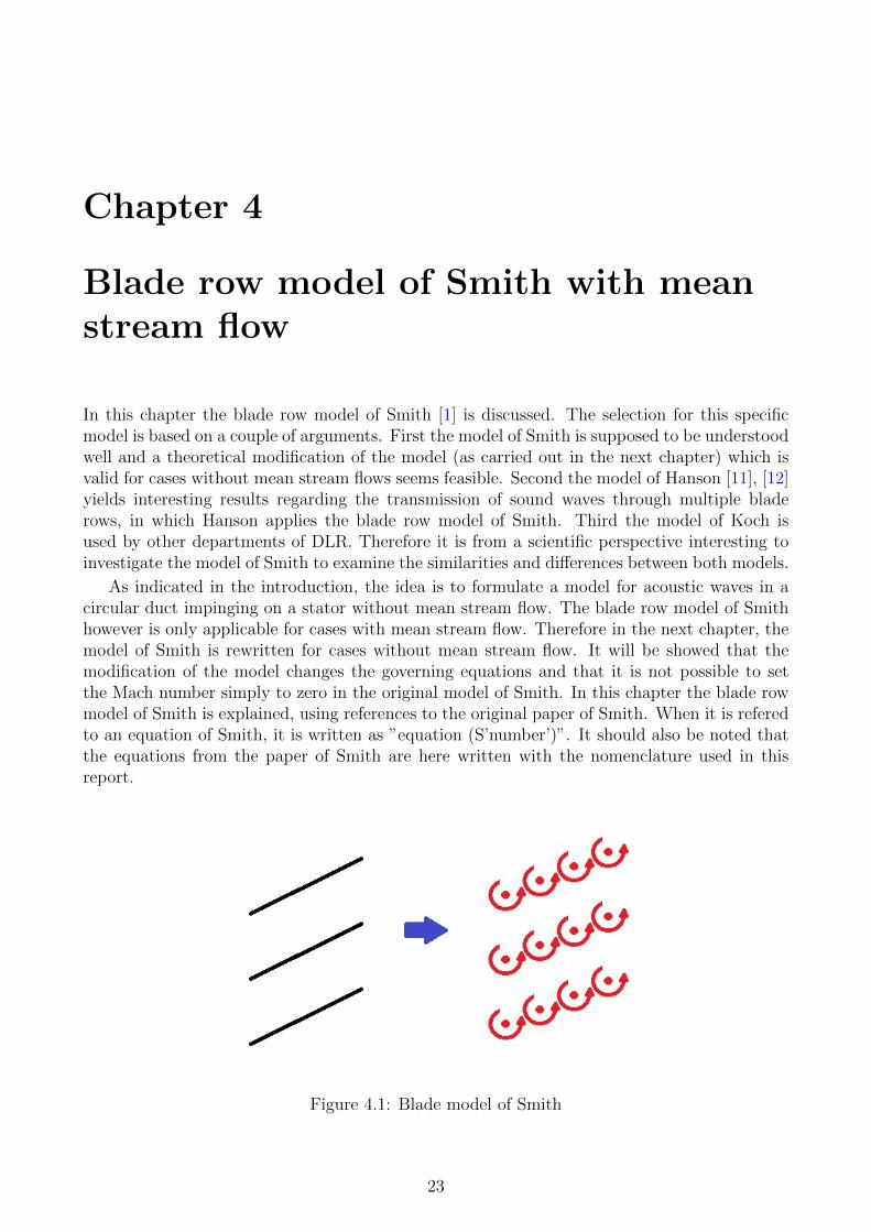
Figure 4.1: Blade model of Smith

23

24 CHAPTER 4. BLADE ROW MODEL OF SMITH WITH MEAN STREAM FLOW

4.1 Principle concept

Consider a pressure wave of a single circumferential wave number m originating far upstreamwith mean flow W impinging on a stator. Note however that the theory discussed in thischapter is also suitable for sound waves impinging on a rotor. It is assumed that the sub-resonant condition is satisfied (k ≤ π

s1−M2

√1−M2 cos2 αs

), indicating there will be no mode scattering

(r = 0 in equation 3.21). Be aware however that, as will be discussed, r = 0 cannot simply beapplied everywhere in the calculation method of Smith.

Smith argues that a blade row can be represented by multiple vortices placed on the bladesurfaces, as visualized in figure 4.1. The principle idea of Smith’s method is the following. Theincoming acoustic wave incident upon the cascade induces a corresponding upwash velocitydistribution on the blades. The upwash velocity is the normal velocity component of thepressure perturbations with respect to the blades. Furthermore the vortices placed on theblades also induce an upwash velocity. Since no air can flow through the blades, the sumof the upwash velocities induced by the incoming pressure wave and by the vortices on theblades should be equal to zero. The vorticity distribution is calculated using the so-calledupwash integral equation, which couples the upwash velocities of the incoming pressure waveand of the vortices. The vorticity distribution is then linked directly to the magnitudes ofthe transmitted and reflected pressure waves, which are used to calculate the transmission andreflection coefficients.

4.2 Governing Equations

Smith starts his paper by making a couple of assumptions. The unwrapped cylindrical ductwith flat plates of negligible thickness (figure 3.1) is used in Smith and the mean stream flowpasses through the cascade undeflected (mean angle of incidence is zero). Furthermore it isassumed that the waves (two velocity components (u and v) and one pressure component (p))are plane waves:

u±m,r = u±m,ri(ω0t+µ

±m,rx+νm,ry)

v±m,r = v±m,rei(ω0t+µ

±m,rx+νm,ry)

p±m,r = p±m,rei(ω0t+µ

±m,rx+νm,ry)

(4.1)

From the linearized equations of continuity and momentum, by assuming the flow is isentropicand the perturbations are indeed plane waves, Smith obtains the characteristic equation (indi-cating non-trivial solutions of the conservation equations) (equation (S6)):[

ω0 + Uµ±m,r + V νm,r] [

(ω0 + Uµ±m,r + V νm,r)2 − a2((µ±m,r)

2 + ν2m,r)

]= 0 (4.2)

From this equation Smith argues that two different physical phenomena are embodied; the termbetween the first square brackets describe vorticity waves, between the second square bracketspressure waves. This indicates that although only acoustic waves hit the blade row, bothpressure waves and vorticity waves, each with different characteristics, need to be consideredfor the evaluation of the transmitted and reflected waves. Or stated different, the incomingpressure wave is not transmitted (or reflected) in pressure waves only, also part of the incomingwave propagates - after hitting the blade row - in the form of a non-acoustic vorticity wave.The characteristics of the pressure and vorticity waves are found using the definition of thevorticity in the flow and the conservation equations. These characteristics are important, sincethey yield ratios between the amplitudes of the velocity and pressure components and therefore

4.3. INCOMING PRESSURE WAVE 25

are used in Smith’s paper to calculate the magnitudes of the far field acoustic waves. Theseratios, given in equation (S9) and (S10), are presented here also:

p±m,rv±m,r

= −(ω0 + Uµ±m,r + V νm,r)ρ0

νm,r(4.3)

u±m,rv±m,r

=µ±m,rνm,r

(4.4)

4.3 Incoming pressure wave

In the paper of Smith, five types of input perturbations are considered. In this report onlyacoustic waves are of interest. Upstream and downstream propagating acoustic wave incidentupon the cascade are stated in Smith. For a downstream propagating acoustic wave, equation(S36) reads:

v−inc,m(x) = −ˆvmeic(µ−inc,m cos(αs)+νinc,m sin(αs))x (4.5)

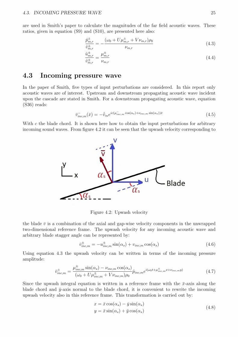
With c the blade chord. It is shown here how to obtain the input perturbations for arbitraryincoming sound waves. From figure 4.2 it can be seen that the upwash velocity corresponding to

Figure 4.2: Upwash velocity

the blade v is a combination of the axial and gap-wise velocity components in the unwrappedtwo-dimensional reference frame. The upwash velocity for any incoming acoustic wave andarbitrary blade stagger angle can be represented by:

v±inc,m = −u±inc,m sin(αs) + vinc,m cos(αs) (4.6)

Using equation 4.3 the upwash velocity can be written in terms of the incoming pressureamplitude:

v±inc,m =µ±inc,m sin(αs)− νinc,m cos(αs)

(ω0 + Uµ±inc,m + V νinc,m)ρ0

pinc,mei(ω0t+µ

±inc,mx+νinc,my) (4.7)

Since the upwash integral equation is written in a reference frame with the x-axis along theblade chord and y-axis normal to the blade chord, it is convenient to rewrite the incomingupwash velocity also in this reference frame. This transformation is carried out by:

x = x cos(αs)− y sin(αs)

y = x sin(αs) + y cos(αs)(4.8)

26 CHAPTER 4. BLADE ROW MODEL OF SMITH WITH MEAN STREAM FLOW

Applying this transformation yields the following expression for the upwash velocity for anarbitrary incoming pressure wave:

v±inc,m =µ±inc,m sin(αs)− νinc,m cos(αs)

(ω0 + Uµ±inc,m + V νinc,m)ρ0

pinc,mei(ω0t+(µ±inc,m cos(αs)+νinc,m sin(αs))x+(−µ±inc,m sin(αs)+νinc,m cos(αs))y)

(4.9)

Which can be written more compact using:

µ±m = µ±m cos(αs) + νm sin(αs)

ν±m = −µ±m sin(αs) + νm cos(αs)(4.10)

With this notation, equation 4.9 is written the following:

v±inc,m = −ν±inc,m

(ω0 + Uµ±inc,m + V νinc,m)ρ0

pinc,mei(ω0t+µ

±inc,mx+νinc,my) (4.11)

An assumption for Smith’s model is that events occurring at any particular blade are dupli-cated at all other blades, with a constant phase angle between each blade and its neighbor.This indicates that the analysis can be carried out on a reference blade, placed on the x-axis.Therefore y = 0, yielding the upwash velocity for an arbitrary downstream propagating incom-ing pressure wave for this reference blade:

v−inc,m = −ν−inc,m

(ω0 + Uµ−inc,m + V νinc,m)ρ0

pinc,mei(ω0t+µ

−inc,mx) (4.12)

Which has indeed the similar appearance as equation 4.5, only now the amplitude is in termsof known and defined quantities.

4.4 Solution for one vortex row

As already indicated, the condition that there is no net upwash at the blade surface shouldbe satisfied (since no air can flow through the blades). Smith derives relations between theunknown vorticity distribution and a given input velocity perturbation (v−inc,m) and betweenthe vorticity distribution and the transmitted and reflected acoustic waves. The vorticitydistribution is solved using the relation with the input velocity perturbation (’upwash integralequation’), from which the result is used to determine the magnitudes corresponding to thetransmitted and reflected acoustic waves.

First step - in order to calculate the transmitted and reflected acoustic waves - is to examinethe conditions to be satisfied by the velocity perturbations produced by the vortices placed onthe blades. These vortices form multiple vortex rows (row in gap-wise direction, with blade gaps between two vortices) which fluctuate in strength with amplitude Γ and angular frequencyω0, with a constant phase angle (inter-vane phase angle) σm between each vortex and its directneighbour on the next blade. The only mention in Smith of the phase angle is done in ”2.1Flow model”, where it is stated that the phase angle is an integral fraction of 2π. It is unclear ifSmith uses the definition of Kaji and Okazaki [4] or a definition similar to that of Jenkins [20],which is discussed in the previous chapter. Here it is assumed that the definition of the inter-vane phase angle is similar as the definition in Jenkins, since the gap-wise wave number ofSmith (equation (S18)) and of Jenkins (Jenkins equation (5.8) are similar and Jenkins statesthat his approach is based on the method of Smith.

4.5. UPWASH INTEGRAL EQUATION 27

From the conditions - which need to be satisfied by the vorticity distribution - the relationbetween the vorticity strength and the magnitudes of the transmitted and reflected acousticwaves is found. These boundary conditions are: 1) the equation of continuity through the bladerow should be satisfied, 2) the velocity jump in y-direction as the cascade is crossed must beequal to the strength of the vortices on the reference blade (Γ) and 3) a relation between thevorticity in the flow and the strength of the vorticity of the bound vortices placed on the bladesmust be satisfied. The total effect of the complete vortex row is presented in Smith (equation(S25)), where the amplitude components are given in equations (S23) and (S24)) and here inequation 4.13 and 4.14. The amplitude components are three different expressions, two for thepressure waves v±m,r and one for the vorticity waves vm,r,vortex.

v±m,r =Γ

s

νm,rc

2A

(∓1∓

(ω0cW

)νm,rc

sinαs +i(ω0cW

)cos(αs)√

(νm,rc)2 −M2A

)(4.13)

vm,r,vortex =Γ

s

(ω0cW

)2+ νm,rc

(ω0cW

)sin(αs)

A(4.14)

With:

W =√U2 + V 2

A =(ω0c

W

)2

+ (νm,rc)2 + 2

(ω0c

W

)νm,rc sin(αs)

(4.15)

An important observation needs to be discussed here concerning equation (S23). In the paperof Smith, the first and third term inside the brackets are dimensionless. However, the secondterm has the dimension of m−1. It is expected that the gap-wise wave number (in Smith β)should be normalized by multiplying it with the chord length c (in Smith β), such that thesecond term between brackets dimensionless. This normalization is applied in this report.

Although for the far field acoustic waves only a specific part of pressure modes are present(other modes are cut-off, these modes decay exponentially), all modes effect the near field(since these modes are not decayed immediately). Therefore in order to calculate the upwashvelocity perturbations induced by the bounded vortices placed on the blades, all pressure modes(r = −∞...∞) need to be considered in the calculation. In terms of the reference frame alongthe chord (x, y) and applied on the reference blade (y=0) this reads:

v±m,r =∞∑

r=−∞

v±m,rei(ω0t+µ

±m,rx) (4.16)

With the amplitude components for pressure perturbations v±m,r or vm,r,vortex for vorticity waves.The dependency of the vorticity strength is implied in these amplitude terms. It should be notedthat this equation describes the contribution of one vortex row of the cascade. In the next partthe complete blade row, containing multiple vortex rows, is considered.

4.5 Upwash integral equation

When the complete blade row is considered, it should be noted that each chordal element dx(with the x-axis along the blades) of the cascade forms a vortex row. The total upwash inducedby the cascade is found by integration along the blade chord, such that the solution is foundnot for one vortex row, but for all vortex rows along the blades. If one carries out integrationalong the chord for equation 4.16 and follows the steps in Smith (”2.6 Derivation of Upwash

28 CHAPTER 4. BLADE ROW MODEL OF SMITH WITH MEAN STREAM FLOW

Integral Equation for cascade”), one finds the upwash integral equation (equation (S30)):

v±m,r(x) =

ˆ 1

0

γ(x0)K(x− x0)dx0 (4.17)

With γ the vorticity strength density and K the so-called Kernel function, defined in equation(S31) and x = 1

cx. Applying this coordinate transformation also for the upwash velocity for

the incoming pressure wave applied on the reference blade (equation 4.12) gives:

v−inc,m(x) = −ν−inc,m

(ω0 + Uµ−inc,m + V νinc,m)ρ0

pinc,mei(ω0t+cµ

−inc,mx) (4.18)

As stated before: The upwash integral equation (equation 4.17) containing the unknown vor-ticity distribution γ can be solved for an arbitrary input velocity distribution (v−inc,m) (equation4.18). This is carried out using a numerical method referred to as a collocation technique. Theequation that needs to be evaluated - since zero net upwash at the blades should be satisfied - is:

−v−inc,m(x) =

ˆ 1

0

γ(x0)K(x− x0)dx0 (4.19)

So the term on the left hand side of the upwash integral equation describes the upwash velocityof the incoming wave and the integral on the right hand side is the upwash velocity due to thebound vortices placed on the blades.

4.6 Far field acoustic waves

When the vorticity distribution is known by solving the upwash integral equation, the magni-tudes of the far field transmitted and reflected acoustic waves (r = 0) can be obtained. Thedependency of the vorticity distribution on the pressure amplitudes is indicated by equation4.13, where the gap-wise velocity component can be rewritten into pressure component follow-ing equation 4.3. Similar as for the upwash integral equation it should also here be noted thateach chordal element of the cascade forms a vortex row which contributes to the magnitudes ofthe transmitted and reflected waves. This procedure, which is indeed similar as the derivationof the upwash integral equation, leads to the total amplitude of the pressure waves (equation(S39)):

p±m = −ρ0W

s/c(v′)±

(ω0cW

)+ µ±mc cos(αs) + νmc sin(αs)

νmc

ˆ 1

0

γ(x0)e−ic(µ±m cos(αs)+νm sin(αs))x0dx0

(4.20)

With v′ is the amplitude term of the gap-wise velocity perturbations (equation 4.13) divided byΓ/s. Or stated differently, this is the amplitude term without the dependency of the vorticitystrength. Inside the exponent in equation (S39) the imaginary number i is only applied on theterm µ±m cos(αs) and not on the second term inside the brackets. It is expected that this is amistake in Smith’s paper, therefore this number i is now written outside of the brackets suchthat is applied on both terms inside these brackets.

4.7 Numerical evaluation upwash integral equation

In order to evaluate the upwash integral equation, another coordinate transformation is conve-nient to carry out. Here a transformation to new independent variables ψ and ε, similar as in

4.7. NUMERICAL EVALUATION UPWASH INTEGRAL EQUATION 29

a usual thin airfoil theory for single airfoils [21]:

x0 =1− cos(ψ)

2

x =1− cos(ε)

2

(4.21)

These new variables are substituted into the upwash integral equation (equation 4.19). Theinterval boundary will change by:

x0 = 1 then 1 =1− cos(ψ)

2(4.22)

yielding :ψ = π (4.23)

The kernel equation will be transformed as follows:

K(x− x0) = K

(1− cos(ε)

2− 1− cos(ψ)

2

)(4.24)

= K

(cos(ψ)− cos(ε)

2

)(4.25)

And dx0 is transformed by:

dx0

dψ=

sin(ψ)

2(4.26)

yielding : dx0 =sin(ψ)

2dψ (4.27)

Substituting all into the upwash integral equation yields:

−v−inc,m(

1− cos(ε)

2

)=

ˆ π

0

γ

(1− cos(ψ)

2

)K

(cos(ψ)− cos(ε)

2

)sin(ψ)

2dψ (4.28)

Next step - in order to evaluate the integral - is to discretize the equation. The bound vorticitycan be specified at (N + 1) points on a uniform spaced grid, given by:

ψ =πl0N

with : l0 = 0, 1, 2, ..., N (4.29)

The value of γ at the trailing edge (l0 = N) is irrelevant since in equation 4.28 it is alwaysmultiplied by sin(ψ) which is zero for l0 = N . However, this argument does not hold forthe leading edge. When solving the upwash integral equation, the vorticity strength γ perunit length will become infinite at the leading edge (l0 = 0). This is also obtained in two-dimensional thin airfoil theory where the Biot-Savart law is used in combination with Glauert’sapproximation (see Anderson [22]) of the integral to calculate the vorticity distribution used formodeling this thin airfoil. So at the leading edge, γ will become infinite but regarding γ sin(ψ)as the fundamental variable this product remains finite at the leading edge and therefore causesno numerical difficulty. This means that the value of γ does not need to be considered at thetrailing edge, but does at the leading edge. Therefore ψ can also be written as:

ψ =πl1N

with : l1 = 0, 1, 2, ..., (N − 1) (4.30)

It is convenient to choose ε - which is related to the points on the grid where the input velocitieswill be defined - such that these values lie midway between the values of ψ at which γ is specified:

ε =π(2l2 + 1)

2Nwith : l2 = 0, 1, 2, ..., (N − 1) (4.31)

30 CHAPTER 4. BLADE ROW MODEL OF SMITH WITH MEAN STREAM FLOW

It is supposed by Whitehead [21] that the upwash integral equation, using the definitions forψ (equation 4.30) and ε (equation 4.31), can be evaluated by the trapezoidal rule. Whiteheadstates that approximating the upwash integral equation using the trapezoidal rule yields re-markably accurate results, although a correction is required for the logarithmic singularity inK if these accurate results are to be obtained with modest values of N [23]. In the paper ofWhitehead [21] the Kernel function is treated such that it is redefined in terms of a modifiedKernel function (which does not contain the troublesome logarithmic singularity) and a termdescribing the logarithmic singularity:

K(..) = K ′(..) +Ksingularity (4.32)

Furthermore Whitehead evaluates this modified Kernel function in his Appendix III [21], wherethe end results is written down in equation (A13) in the paper of Whitehead. It is expectedthat Smith, although not written explicitly, uses this modified Kernel function such that theupwash integral equation becomes:

N∑l1=0

′

γ(1− cos(πl1N

)2

)K ′

cos(πl1N

)− cos

(π(2l2+1)

2N

)2

π

2Nsin

(πl1N

)= −v−inc,m

1− cos(π(2l2+1)

2N

)2

(4.33)

With∑N

l1=0′ denoting a summation in which the first and last terms are given half weight

(consequence of trapezoidal rule). It should be noted that the notation of Smith and Whiteheadcan be confusing, they use a vinculum to group 2l2 + 1. It is confusing since this is a notationwhich is not used often in present days. This equation may be written in matrix-vector notationas:

[K]Γ = v (4.34)

Where [K] is a N ×N matrix with the element in the lth2 row and lth1 column given by:

K ′

cos(πl1N

)− cos

(π(2l2+1)

2N

)2

(4.35)

Again stated, this modified Kernel function is not defined in Smith and is not completely similarto the analytic Kernel function of equation (S31). It is the modified expression of this Kernelfunction, without the logarithmic singularity which is present in the analytic Kernel function.The vector Γ is a N × 1 vector with the lth1 entry given by:

π

2Nsin

(πl1N

)γ

(1− cos

(πl1N

)2

)(4.36)

And v is also a N × 1 vector with the lth2 entry given by:

−v−inc,m

1− cos(π(2l2+1)

2N

)2

(4.37)

The direct solution of equation 4.34 is:

Γ = [K]−1v (4.38)

4.8. NUMERICAL EVALUATION ACOUSTIC WAVE AMPLITUDES 31

4.8 Numerical evaluation acoustic wave amplitudes

When Γ is calculated, the magnitudes of the transmitted and reflected transmitted pressurewaves can be calculated using a numerical modification of equation 4.20. Once again, since itcan be confusing, the difference in using r is explained. For calculating the vorticity distributionΓ using the upwash integral equation (equation 4.38), all pressure modes need to be considered(r = −∞...∞). However for calculating the magnitudes of the transmitted and reflected trans-mitted far field acoustic waves waves where the sub-resonance condition is satisfied: r = 0. Inorder to solve the integral in equation 4.20 numerically, again the trapezoidal rule is carriedout for calculating the pressure wave amplitudes:

p±m =− ρ0W

s/c(v′)±

(ω0cW

)+ µ±mc cos(αs) + νmc sin(αs)

νmc

n∑l1=0

′[π

2nsin

(πl1N

)γ

]e−icµ±m(

1−cos(πl1N

)

2

) (4.39)

With the magnitudes of the far field acoustic waves known, the transmission and reflectioncoefficients can be calculated using equation 3.39.

32 CHAPTER 4. BLADE ROW MODEL OF SMITH WITH MEAN STREAM FLOW

Chapter 5

Blade row model of Smith withoutmean stream flow

As already indicated in the previous chapter, the flow velocity cannot simply be set to zeroin the model of Smith. This can be seen by setting W to zero in equation 4.13, the ampli-tudes - according to the model of Smith - will be infinite which is not physical. A couple ofdifferences are summed here. The first difference can already be observed in the characteristicequation from the linearized equations of continuity and momentum (equation 4.2). Whenthe fluid velocity is zero, there are no vorticity waves present. Only ω0 = 0 yields non-trivialsolutions. Since there are no vorticity waves, the third boundary condition (a relation betweenthe vorticity in the flow and the strength of the vorticity of the bound vortices placed on theblades) discussed in ”4.4 Solution of one vortex row” cannot be used. This has the consequencethat the amplitudes components for the transmitted and reflected waves (v±m in equation 4.13)cannot be used from Smith. Finally this changes the Kernel function in the upwash integralequation (equation 4.19) and therefore the modified Kernel function of Whitehead [21] cannotbe applied. Moreover, since the governing conservation equations are different, the ratios ofthe velocity and pressure amplitude components are different (equation 4.3). Therefore alsothe calculation of the total amplitude of the pressure wave (equation 4.20) is different. Thesedifferences indicate, that for a case without mean stream flow, the model needs to be ’build’from the same starting point as Smith carried out: the governing equations.

5.1 Governing equations

Again a pressure wave of a single circumferential wave number m originating far upstreamimpinging on a stator is considered, only now without mean flow. It is still assumed thatthe sub-resonant condition is satisfied (k ≤ π

s). The linearized equations of continuity and

momentum without mean stream flow read, assuming the medium is isentropic:

∂p

∂t+ ρ0a

2

(∂u

∂x+∂v

∂y

)= 0

∂u

∂t= − 1

ρ0

∂p

∂x∂v

∂t= − 1

ρ0

∂p

∂y

(5.1)

Also it is assumed the the perturbations are plane waves (equation 4.1). From these statements,the characteristic equation for non-trivial solutions of the conservation equation is found:

(ω0 + Uµ±m,r + V νm,r)2 − a2((µ±m,r)

2 + ν2m,r) = 0 (5.2)

33

34 CHAPTER 5. BLADE ROW MODEL OF SMITH WITHOUT MEAN STREAM FLOW

When this is compared with the characteristic equation of the model of Smith with mean streamflow (equation 4.2), it is indeed observed that only pressure waves are present. The ratios ofthe amplitudes of the velocity and pressure components are similar as equation 4.3, but for thefact the mean stream flow is set to zero:

p±m,rv±m,r

= −ω0ρ0

νm,r

u±m,rv±m,r

=µ±m,rνm,r

(5.3)

5.2 Incoming pressure wave

The calculation method for the incoming pressure wave is identical, since it is not directly linkedto the method of Smith. However, since the ratios between the amplitudes of the velocity andpressure components are different, the incoming upwash velocity is a bit different. Applyingthe definition of the upwash velocity (equation 4.6), carrying out the coordinate transforma-tion such that the x-axis is placed along the blade chord and y-axis normal to the blade chord(equation 4.8), using the convention of µ±m and ν±m of equation 4.10 and carry out the analysison the reference blade (y = 0) the upwash velocity for an arbitrary incoming pressure wave,propagating in downstream direction, without mean stream flow yields:

v−inc,m = −ν−inc,mω0ρ0

pinc,mei(ω0t+µ

−inc,mx) (5.4)

5.3 Solution of one vortex row

Next step in the method of Smith is to find the solution of one vortex row of the blade row. Theboundary conditions used in Smith’s paper cannot be used similarly. As already indicated, thecondition that there is no net upwash at the blade surface should be satisfied (since no air canflow through the blades). For the sake of clarity the axial and gap-wise velocity components inthe (x,y) reference frame are derived using the ratios between the amplitudes of the velocityand pressure components 5.3. Note that these are velocity perturbations produced by thevortices. Already discussed in the previous chapter, although for the far field acoustic wavesonly a specific part of pressure modes are present, all modes are effecting the near field:

u±m,r = −µ±m,rω0ρ0

p±m,rei(ω0t+µ

±m,rx+νm,ry)

v±m,r = − νm,rω0ρ0

p±m,rei(ω0t+µ

±m,rx+νm,ry)

(5.5)

First condition applied on the velocity perturbations produced by these vortices is theequation of continuity through the cascade. The vortices produce up- and downstream pressurewaves. Therefore in order to satisfy the equation of continuity, the magnitudes of the axialvelocity perturbations at the cascade should be equal:

µ+m,r

ω0ρ0

p+m,r −

µ−m,rω0ρ0

p−m,r = 0 (5.6)

From the relation of the axial wave number (equation 3.9), setting the Mach numbers to zero,it is found that:

µ+m,r = −µ−m,r (5.7)

5.4. UPWASH INTEGRAL EQUATION 35

Plugging this into equation 5.6:

p+m,r + p−m,r = 0 (5.8)

The second condition comes from the velocity jump in y-direction as the cascade is crossed.This velocity jump should be similar to the strength of the vortices on blades (Γ):

p+m,r − p−m,r =

ω0ρ0

νm,r

Γ

s(5.9)

Equation 5.8 and 5.9 yield the magnitude of the transmitted (-) and reflected (+) pressurewaves:

p± = ± ω0ρ0

2νm,r

Γ

s(5.10)

The magnitudes of the transmitted and reflected pressure waves now also depend on the strengthof the vorticity and the blade gap. Substituting this into equation 4.1 yields the relations forthe transmitted and reflected pressure waves. In terms of the reference frame along the chord(x,y) and applied on the reference blade (y=0) this reads:

p±m,r(x, t) = ±Γ

s

ω0ρ0

2νm,rei(ω0t+µ

±m,rx) (5.11)

5.4 Upwash integral equation

For the derivation of the upwash integral equation the similar approach as in the previouschapter (and therefore similar to the method of Smith) is carried out. Using the ratio betweenthe pressure amplitude and the gap-wise velocity amplitude (equation 5.3) the induced upwashvelocities at the point x on the reference blade is found:

v±m,r(x) = ±1

2

γ(x0)dx0

s

∞∑r=−∞

ei(ω0t+µ±m,r(x−x0)) (5.12)

The relevant velocities for (x − x0) < 0 are those associated with the upstream pressure per-turbation (+); for (x − x0) > 0 those associated with the downstream pressure perturbation(-). The total upwash induced by the cascade is found by integration along the blade chord:

v±m,r(x) = −ˆ x

0

γ(x0)

2s

∞∑r=−∞

ei(ω0t+µ−m,r(x−x0))dx0

−ˆ c

x

γ(x0)

2s

∞∑r=−∞

ei(ω0t+µ+m,r(x−x0))dx0

(5.13)

This relation can be rewritten using a convenient coordinate transformation x = 1cx in order

to obtain a dimensionless interval for the integral. Also here the summation of the upwashvelocity corresponding to the bound vortices and the incoming pressure waves, respectively,should be zero. Applying this leads to:

−v±inc,m(x) =

ˆ 1

0

γ(x0)K(x− x0)dx0

with : K(η) = − 1

(2s/c)

∞∑r=−∞

ei(ω0t+cµ−m,rη) for η > 0

and : K(η) = − 1

(2s/c)

∞∑r=−∞

ei(ω0t+cµ+m,rη) for η < 0

(5.14)

36 CHAPTER 5. BLADE ROW MODEL OF SMITH WITHOUT MEAN STREAM FLOW

Which is a similar looking equation as the upwash integral equation for the method of Smithwith free stream flow (equation 4.19). However be aware that the Kernel function is differentfor the two cases.

5.5 Far field acoustic waves

Solving the upwash integral equation yields the vorticity distribution, which is used to calcu-late the magnitudes of the far field acoustic waves. This is carried out using equation 5.11 andthe definition of the plane wave (equation 4.1) for which should be observed that each chordalelement of the cascade forms a vortex row contributing to the magnitudes of the waves:

p±m,r = ± ω0ρ0

2νm,r

Γ

se−iµ

±m,rx0

= ± ω0ρ0

νm,r(2s/c)

ˆ 1

0

γ(x0)e−iµ±m,rx0dx0

(5.15)

Which is again quite similar equation 4.20, but for differences concerning the absence of meanstream velocity.

5.6 Numerical evaluation upwash integral equation and

acoustic wave amplitudes

The same collocation technique is carried out to solve the upwash integral equation. Carryingout the coordinate transformation of equation 4.21 on the upwash integral equation (equation5.14), setting ψ and ε following equations 4.30 and 4.31 and applying the trapezoidal rule yields:

n∑l1=0

′

γ(1− cos(πl1n

)2

)K ′

cos(πl1n

)− cos

(π(2l2+1)

2n

)2

π

2nsin

(πl1n

)= −v−inc,m

1− cos(π(2l2+1)

2n

)2

(5.16)

Similar as equation 4.34, this may be written in matrix-vector notation:

[K]Γ = v (5.17)

With the direct solution:

Γ = [K]−1v (5.18)

In the original paper of Smith, the Kernel function is corrected such that accurate resultsare to be obtained with modest values of N . One can try to carry out a similar correctionby finding a modified Kernel function for the case without mean stream flow by investigatingthe calculation method of Whitehead carefully. However, it is stated in a review article ofWhitehead in 1987 [23] that this correction of the Kernel is required such that accurate resultswith modest values of N is obtained. This also suggest that the Kernel function (includingthe logarithmic singularity) should yield accurate results for large values of N and therefore inprinciple can be solved using equation 5.18.

5.6. NUMERICAL EVALUATION UPWASH INTEGRAL EQUATION ANDACOUSTICWAVE AMPLITUDES37

With the vorticity distribution obtained, the magnitudes of the far field acoustic waves canbe calculated using the numerical modification of equation 5.15:

p±m,r =± ω0ρ0

νm,r(2s/c)

n∑l1=0

′[π

2nsin

(πl1n

)γ

]e−icµ±m,r(

1−cos(πl1n )

2

) (5.19)

The transmission and reflection coefficients are obtained by applying the results of this pro-cedure (the amplitudes of the transmitted and reflected power waves) in the relations for thecoefficient (equation 3.39).

38 CHAPTER 5. BLADE ROW MODEL OF SMITH WITHOUT MEAN STREAM FLOW

Chapter 6

Results

In this chapter the preliminary results of the original model of Smith - with mean streamflow - is discussed. In order to enhance the readability of this chapter, the course of eventsis explained. In the time available, it was first attempted to carry out calculations for themodified model of Smith, since experiments without mean stream flow are planned at DLR.However, the results using an implemented calculation program with MATLAB did not yieldsatisfactory results. Therefore it is thought to duplicate the calculations carried out by Smith,such that the validity of the calculation program can be investigated and to give more insight inthe possible unforeseen difficulties arising when the theoretical model is implemented. In thischapter typical results of the blade row models of the 1970’s (see literature review in chapter 2)is presented, the implemented MATLAB program is explained and the raw results are discussed.Since the results of the duplicated model of Smith do not yield satisfactory results, it cannotbe expected to find accurate results for the model without mean stream flow. Therefore onlythe results of the current program which calculates the transmission and reflection coefficientsfollowing the original model of Smith are presented and discussed in this report.

6.1 Typical results of blade row models

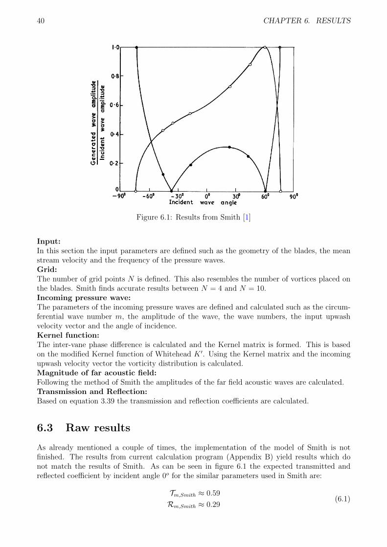
As is indicated in the literature review, Kaji and Okazaki were the pioneers examining thesubject of the transmission of sound waves through blade rows. The blade row models definedafter Kaji and Okazaki in the 1970’s (Smith, Koch, Amiet, a.o.) presented the transmissionand reflection coefficients such that they can compare their results with the results of Kaji andOkazaki. The results of the transmission and reflection coefficients from Smith are visualized infigure 6.1. The results from Smith are for an upstream propagating incident wave with s/c = 1,the blade stagger angle of 60o, the flow Mach number 0.5 and an in Smith defined frequencyparameter λ = π/2. The black lines present the results of Kaji and Okazaki [4], the open andclosed circles represent the transmission and reflection coefficients from the calculation methodof Smith. Since similar parameters are used, it is expected that the calculation program,implementing the original method of Smith yields similar results as displayed in figure 6.1.

6.2 Implementation in MATLAB

The model of Smith is implemented in MATLAB using three files: ’Main upstream’, ’Kernelwhitehead’ and ’V whitehead’. The main file contains most implementation of the model ofSmith, the file containing the Kernel function calculates every index for the modified Kernelmatrix (equation 4.35) in which the function V from the paper of Whitehead [21] is applied.These files can be found in Appendix B. Here an overview of the MATLAB program is given:

39

40 CHAPTER 6. RESULTS

Figure 6.1: Results from Smith [1]

Input:In this section the input parameters are defined such as the geometry of the blades, the meanstream velocity and the frequency of the pressure waves.Grid:The number of grid points N is defined. This also resembles the number of vortices placed onthe blades. Smith finds accurate results between N = 4 and N = 10.Incoming pressure wave:The parameters of the incoming pressure waves are defined and calculated such as the circum-ferential wave number m, the amplitude of the wave, the wave numbers, the input upwashvelocity vector and the angle of incidence.Kernel function:The inter-vane phase difference is calculated and the Kernel matrix is formed. This is basedon the modified Kernel function of Whitehead K ′. Using the Kernel matrix and the incomingupwash velocity vector the vorticity distribution is calculated.Magnitude of far acoustic field:Following the method of Smith the amplitudes of the far field acoustic waves are calculated.Transmission and Reflection:Based on equation 3.39 the transmission and reflection coefficients are calculated.

6.3 Raw results

As already mentioned a couple of times, the implementation of the model of Smith is notfinished. The results from current calculation program (Appendix B) yield results which donot match the results of Smith. As can be seen in figure 6.1 the expected transmitted andreflected coefficient by incident angle 0o for the similar parameters used in Smith are:

Tm,Smith ≈ 0.59

Rm,Smith ≈ 0.29(6.1)

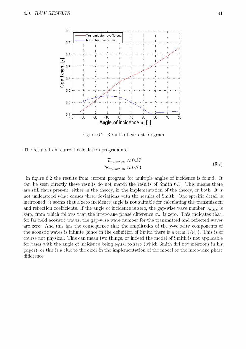
6.3. RAW RESULTS 41

Figure 6.2: Results of current program

The results from current calculation program are:

Tm,current ≈ 0.37

Rm,current ≈ 0.23(6.2)

In figure 6.2 the results from current program for multiple angles of incidence is found. Itcan be seen directly these results do not match the results of Smith 6.1. This means thereare still flaws present; either in the theory, in the implementation of the theory, or both. It isnot understood what causes these deviations with the results of Smith. One specific detail ismentioned; it seems that a zero incidence angle is not suitable for calculating the transmissionand reflection coefficients. If the angle of incidence is zero, the gap-wise wave number νm,inc iszero, from which follows that the inter-vane phase difference σm is zero. This indicates that,for far field acoustic waves, the gap-wise wave number for the transmitted and reflected wavesare zero. And this has the consequence that the amplitudes of the y-velocity components ofthe acoustic waves is infinite (since in the definition of Smith there is a term 1/νm). This is ofcourse not physical. This can mean two things, or indeed the model of Smith is not applicablefor cases with the angle of incidence being equal to zero (which Smith did not mentions in hispaper), or this is a clue to the error in the implementation of the model or the inter-vane phasedifference.

42 CHAPTER 6. RESULTS

Chapter 7

Conclusion

7.1 Main conclusions

The first objective of the present study was to carry out a review of literature regarding existinganalytical models that describe the propagation of sounds waves through turbomachinery bladerows. From this analysis it is found that analytical models are defined in the 1970’s with KajiOkazaki [5], [4] as pioneers in this field. Two models (Smith [1] and Koch [7]) are used often inliterature after the 1970’s, both using different mathematical tools to describe the sound wavesthrough blade rows. Also other phenomena, such as mode trapping and acoustic resonance arediscussed in literature. These effect should be considered when calculation models for multipleblade rows are defined.

The theory of the blade row model of Smith is discussed in chapter 4, from which it isfound that the paper of Smith can only be understood correctly with knowledge of the modelof Whitehead [21]. A modification of Smith’s blade row model is presented in chapter 5, whichis supposed to be theoretically valid. The implementation of the original and the modifiedmodel of Smith is not complete, there are still flaws in the understanding of the theory, theimplementation of the model, or both. However, since Smith presents results in his paper, itis believed that the understanding of the theory and/or the implementation of the model isachievable. It should also be noted, since the implementation of the modified model is lacking,the validity of the theoretical modification of the blade row model of Smith is not checked.When applying the modified model, one should be aware of this fact.

7.2 Recommendations

The most significant development that needs to be carried out is to find the errors in the currentcalculation program. The only hint, which is also discussed in the results, of a possible erroris the disability of the current program to cope with a zero incidence angle. More examinationof the model in Smith for deeper understanding and better implementation is therefore recom-mended. When the calculation program for the original model of Smith is valid, the attentioncan shift towards implementation of the modified model of Smith. The results from the mod-ified model are recommended to use for examining the validity of the theoretical modificationof the blade row model.

If the calculation program for the modified blade row model is operational, experiments canbe conducted for sound waves propagating through ducted turbomachinery blade rows. It isadvised to investigate the comparisons and differences between the results from the (modified)model of Smith and experiments. Future research should enhance the understanding of soundwaves propagating through blade rows, which can be applied in other studies, for example in

43

44 CHAPTER 7. CONCLUSION

studies on noise reduction for airplane engines.

Bibliography

[1] S. Smith, “Discrete frequency sound generation in axial flow turbomachines,” AeronauticalResearch Council Reports and Memoranda, 1972.

[2] S. Glegg, “The response of a swept blade row to a three-dimensional gust,” Journal ofsound and vibration, vol. 227, no. 1, pp. 29–64, 1999.

[3] R. Muir, “The application of a semi-actuator disk model to sound transmission calculationsin turbomachinery, part i: The single blade row,” Journal of Sound and Vibration, vol. 54,no. 3, pp. 393–408, 1977.

[4] S. Kaji and T. Okazaki, “Propagation of sound waves through a blade row: Ii. analysisbased on the acceleration potential method,” Journal of Sound and Vibration, vol. 11,no. 3, pp. 355 – IN1, 1970.

[5] S. Kaji and T. Okazaki, “Propagation of sound waves through a blade row: I. analysisbased on the semi-actuator disk theory,” Journal of Sound and Vibration, vol. 11, no. 3,pp. 339 – 353, 1970.

[6] R. Mani and G. Horvay, “Sound transmission through blade rows,” Journal of sound andvibration, vol. 12, no. 1, pp. 59–83, 1970.

[7] W. Koch, “On the transmission of sound waves through a blade row,” Journal of soundand vibration, vol. 18, no. 1, pp. 111–128, 1971.

[8] R. Amiet, “Transmission and reflection of sound by a blade row,” AIAA Journal, vol. 9,no. 10, pp. 1893–1894, 1971.

[9] D. Topol, S. Holhubner, and D. Mathews, “A reflection mechanism for aft fan tone noisefrom turbofan engines,” in American Institute of Aeronautics and Astronautics Conference,vol. 1, 1987.

[10] J. M. Tyler and T. G. Sofrin, “Axial flow compressor noise studies,” tech. rep., SAETechnical Paper, 1962.

[11] D. Hanson, “Mode trapping in coupled 2d cascades-acoustic and aerodynamic results,”AIAA Paper, no. 93-4417, 1993.

[12] D. B. Hanson, “Acoustic reflection and transmission of 2-dimensional rotors and stators,including mode and frequency scattering effects,” AIAA Paper, 1999.

[13] D. B. Hanson, “Broadband noise of fans-with unsteady coupling theory to account for ro-tor and stator reflection/transmission effects,” Contractor report NASA, no. 2001-210762,2001.

45

46 BIBLIOGRAPHY

[14] H. Posson, H. Beriot, and S. Moreau, “On the use of an analytical cascade responsefunction to predict sound transmission through an annular cascade,” Journal of Soundand Vibration, vol. 332, no. 15, pp. 3706–3739, 2013.

[15] D. A. Topol, “Development and evaluation of a coupled fan noise design system,” AIAAPaper, no. 97-1611, 1997.

[16] P. D. Silkowski and K. C. Hall, “1997 best paper award - structures and dynamics commit-tee: A coupled mode analysis of unsteady multistage flows in turbomachinery,” Journal ofturbomachinery, vol. 120, no. 3, pp. 410–421, 1998.

[17] R. Parker, “Acoustic resonances and blade vibration in axial flow compressors,” Journalof Sound and Vibration, vol. 92, no. 4, pp. 529–539, 1984.

[18] B. Hellmich and J. R. Seume, “Causes of acoustic resonance in a high-speed axial com-pressor,” Journal of Turbomachinery, vol. 130, no. 3, 2008.

[19] W. Neise and U. Michel, Aerodynamics Noise of Turbomachines. DLR Internal Report22314-94/B5, Institute of Propulsion Technology, Department of Engine Acoustics, 1994.

[20] G. Jenkins, Models for the prediction of rear-arc and forward-arc fan broadband noise inturbofan engines. PhD thesis, University of Southampton, 2013.

[21] D. S. Whitehead, Force and moment coefficients for vibrating aerofoils in cascade. HMStationery Office, 1962.

[22] J. Anderson, Fundamentals of Aerodynamics. McGraw-Hill Series in Aeronautical and,McGraw-Hill Higher Education, 4 ed., 2007.

[23] D. Whitehead, “Classical two-dimensional methods,” In AGARD Aeroelasticity in Axial-Flow Turbomachines., vol. 1, 1987.

[24] A. Fritzsch, “Numerische untersuchung der transmission, reflexion und streuung von schall-wellen an einem schaufelgitter,” Master’s thesis, Technische Universitat Berlin, Institut furStromungsmechanik und Technische Akustik, 2009.

Appendix A

Power coefficients

The second definition is the ratio of the acoustic powers of the transmitted, reflected andincoming sound waves, for example used in Hanson [11], [12]. A measure of the energy of soundper time unit is called the acoustic or sound power. This acoustic power is defined as the soundintensity (sound power per area) times the corresponding area. For a circular duct, unwrappedinto the two-dimensional reference frame, it reads:

P± =

2πˆ

0

I±x R0dφ =

Bsˆ

0

I±x dy (A.1)

With Ix the sound intensity in axial direction. The intensity is not really integrated over asurface, but over a line. This power can therefore also be interpreted as a power density of thesound. The sound intensity for a pressure wave with zero mean flow is defined as [24]:

I±x =1

2<(p∗u) (A.2)

=

∣∣∣∣12(preure + pimuim)

∣∣∣∣ (A.3)

With subscript re stating the real part and the imaginary part is noted with subscript im. Thevelocity perturbations can be obtained applying the linearized x-momentum equation for zeromean flow, here carried out for the transmitted and reflected pressure waves from a stator whenthe sub-resonance condition 3.12 is satisfied. Note however that the same analysis can also becarried out for rotors and for super-resonance conditions:

∂u

∂t= − 1

ρ0

∂p

∂x(A.4)

With the mean density of the medium ρ0. Using this relation, the axial velocity perturbationis found:

u±m = − µ±mω0ρ0

p±mei(ω0t+µ

±mx+νmy) (A.5)

With this the pressure and velocity perturbations are known, these are plugged into the defi-nition of the axial intensity (equation A.3), which is then substituted into the equation for theacoustic power (equation A.1):

P± =

Bsˆ

0

∣∣∣∣12 µ±mω0ρo

(p±m)2

∣∣∣∣ dy (A.6)

=

∣∣∣∣12 µ±mBsω0ρo(p±m)2

∣∣∣∣ (A.7)

47

48 APPENDIX A. POWER COEFFICIENTS

Similar procedure can be carried out for the incoming pressure wave. This yields:

Pinc =

∣∣∣∣∣µ−inc,mBsω0ρo(pinc,m)2

∣∣∣∣∣ (A.8)

The transmission and reflection coefficients are ratios of the transmitted/reflected acousticpower and the incoming acoustic power [11]. Using this definition, the transmission coefficientfor the pressure wave modes impinging on a stator with zero mean flow is:

Tm =P−

Pinc=

∣∣∣∣∣ µ−m(p−m)2

µ−inc,m(pinc,m)2

∣∣∣∣∣ (A.9)

And the reflection coefficient:

Rm =P+

Pinc=

∣∣∣∣∣ µ+m(p+

m)2

µ−inc,m(pinc,m)2

∣∣∣∣∣ (A.10)

The relation for the reflection coefficient can be rewritten into a representation from whichthe validity of both relations (transmission and reflection) can be verified. This is done bynoting that the acoustic power of the incoming pressure wave and the transmitted and reflectedpressure waves are related to each other. Assuming that the blade row does not produce ordissipates energy, the acoustic power of the incoming pressure wave should equal the sum ofthe acoustic power of the transmitted and reflected pressure waves:

Pinc = P− + P+ (A.11)

Substituting the expressions for the acoustic power (equation A.8 and A.7) yields:∣∣µ−inc,m(pinc,m)2∣∣ =

∣∣µ−m(p−m)2∣∣+∣∣µ+m(p+

m)2∣∣ (A.12)

Substituting then this equation (A.12) into the relation for the reflection coefficient (equationA.10) gives:

Rm =

∣∣∣∣∣ µ+m(p+

m)2

µ−inc,m(pinc,m)2

∣∣∣∣∣ =

∣∣∣∣∣µ−inc,m(pinc,m)2 − µ−m(p−m)2

µ−inc,m(pinc,m)2

∣∣∣∣∣ = 1− Tm (A.13)

So for the case of total transmission (all of the acoustic power of the incoming pressure wavetransmits through the blade row), the transmission coefficient Tm is one, implying that thereflection coefficient Rm is zero, which fulfills the expectation.

Appendix B

MATLAB scripts

B.1 Main upstream

1 close all2 clear all3 clc4

5 %% Input Parameters6

7 B = 25 ; % [-] Number of blades of stator8 R = 0.25 ; % [m] Radius of blades9 s = 2*pi*R/B ; % [m] Blade Gap

10 c = s; % [m] Blade Chord11

12 Um = 85; % [m/s] Axial Free stream velocity13 Vm = Um*1.73; % [m/s] Gap-Wise Free stream velocity14 W = sqrt(Umˆ2+Vmˆ2);% [m/s] Mean stream flow15 a = 343 ; % [m/s] Speed of sound16 M = W/a ; % [-] Mach Number17

18 as = atan(Vm/Um) ; % [rad] Stagger angle19

20 w = 2*pi*675; % [rad/s] Acoustic frequency21 rho = 1.2 ; % [kg/mˆ3] Density of fluid22

23 l = w*c/W ; % [-] Frequency parameter24 wl = 2*pi*a/w; % [m] Wave length25

26 k = w/a ; % [-] Wave number27

28 %% Display29

30 disp(' Sub -Resonance? ')31

32 if (k)<=(pi/s*(1-Mˆ2)/sqrt(1-Mˆ2*cos(as)ˆ2))33 fprintf('yes! \n')34 fprintf('%.2f (w/a) <= %.2f (pi/s*(1-Mˆ2)/sqrt(1-Mˆ2*cos(as)ˆ2))\n \n'35 ,w/a,pi/s*(1-Mˆ2)/sqrt(1-Mˆ2*cos(as)ˆ2))36 end37 disp(' Compare with Smith: ')38 fprintf('as = %.0f (stagger angle)\n',as*180/pi)39 fprintf('s/c = %.2f (gap/chord)\n',s/c)40 fprintf('M = %.2f (Mach Number)\n',M)

49

50 APPENDIX B. MATLAB SCRIPTS

41 fprintf('l = %.2f (Frequency parameter)\n',l)42 fprintf('wl = %.2f (Wave Length)\n',wl)43 fprintf('wl/c= %.2f (Wave Length/chord)\n',wl/c)44

45 %% Grid46 n = 10 ; % Number of grid points47 range = 0:(n-1) ;48

49 fprintf('n = %.0f (Number of grid points)\n',n)50

51 %% Incoming acoustic wave52

53 m = 0.01 ; % [-] Circumferential wave number54 P inc = 1 ; % [N/mˆ2] Magnitude of incoming acoustic wave55

56 fprintf('m = %1.f (circumferential mode order)\n',m)57

58 % Incoming acoustic field59 nu inc = 2*pi*m/(B*s) ; % Gap wise wave number60 f1 = w+Vm*nu inc ; % component in axial wave number61 f2 = aˆ2-Umˆ2 ; % component in axial wave number62 mu inc = (Um*f1+a*sqrt(f1ˆ2-f2*nu incˆ2))/f2 ; % Axial wave number63

64 if imag(mu inc) ~= 065 display(' ')66 display('Error: Incoming pressure wave is cut-off!')67 display(' ')68 end69

70 % Calculating the incoming upwash velocity vector71 range2 = range(:) ;72 eta = (1-cos(pi*(2*range2+1)/(2*n)))/2 ;73

74 f1 = P inc/((w+Um*mu inc+Vm*nu inc)*rho) ;75 f2 = mu inc*sin(as)-nu inc*cos(as) ;76 f3 = 1i*c*eta*(mu inc*cos(as)+nu inc*sin(as)) ;77 V = -f1*f2*exp(f3) ;78

79 aw = atan(-nu inc/mu inc) ;80 fprintf('aw = %.0f (Incident wave angle)\n\n',aw*180/pi)81

82 %% Kernel Function83

84 % Inter-vane-phase-difference85 sigma = nu inc*s;86

87 % Input for the Kernel Function (whitehead)88 ak = c/s*cos(as) ;89 bk = c/s*sin(as) ;90

91 K = zeros(n,n) ;92

93 % Calculating the terms of Kernel Matrix94 for l2 = range95 for l1 = range96 eta = 1/2*(cos(pi*l1/n)-cos(pi*(2*l2+1)/(2*n))) ;97 K(l2+1,l1+1)=Kernel whitehead(eta,l,sigma,ak,bk,n,l1) ;98 end99 end

100

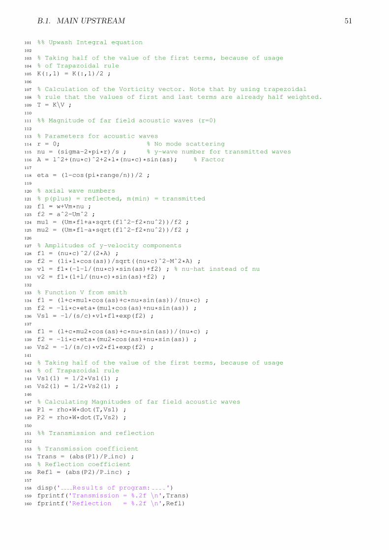
B.1. MAIN UPSTREAM 51

101 %% Upwash Integral equation102

103 % Taking half of the value of the first terms, because of usage104 % of Trapazoidal rule105 K(:,1) = K(:,1)/2 ;106

107 % Calculation of the Vorticity vector. Note that by using trapezoidal108 % rule that the values of first and last terms are already half weighted.109 T = K\V ;110

111 %% Magnitude of far field acoustic waves (r=0)112

113 % Parameters for acoustic waves114 r = 0; % No mode scattering115 nu = (sigma-2*pi*r)/s ; % y-wave number for transmitted waves116 A = lˆ2+(nu*c)ˆ2+2*l*(nu*c)*sin(as); % Factor117

118 eta = (1-cos(pi*range/n))/2 ;119

120 % axial wave numbers121 % p(plus) = reflected, m(min) = transmitted122 f1 = w+Vm*nu ;123 f2 = aˆ2-Umˆ2 ;124 mu1 = (Um*f1+a*sqrt(f1ˆ2-f2*nuˆ2))/f2 ;125 mu2 = (Um*f1-a*sqrt(f1ˆ2-f2*nuˆ2))/f2 ;126

127 % Amplitudes of y-velocity components128 f1 = (nu*c)ˆ2/(2*A) ;129 f2 = (1i*l*cos(as))/sqrt((nu*c)ˆ2-Mˆ2*A) ;130 v1 = f1*(-1-l/(nu*c)*sin(as)+f2) ; % nu-hat instead of nu131 v2 = f1*(1+l/(nu*c)*sin(as)+f2) ;132

133 % Function V from smith134 f1 = (l+c*mu1*cos(as)+c*nu*sin(as))/(nu*c) ;135 f2 = -1i*c*eta*(mu1*cos(as)+nu*sin(as)) ;136 Vs1 = -1/(s/c)*v1*f1*exp(f2) ;137

138 f1 = (l+c*mu2*cos(as)+c*nu*sin(as))/(nu*c) ;139 f2 = -1i*c*eta*(mu2*cos(as)+nu*sin(as)) ;140 Vs2 = -1/(s/c)*v2*f1*exp(f2) ;141

142 % Taking half of the value of the first terms, because of usage143 % of Trapazoidal rule144 Vs1(1) = 1/2*Vs1(1) ;145 Vs2(1) = 1/2*Vs2(1) ;146

147 % Calculating Magnitudes of far field acoustic waves148 P1 = rho*W*dot(T,Vs1) ;149 P2 = rho*W*dot(T,Vs2) ;150

151 %% Transmission and reflection152

153 % Transmission coefficient154 Trans = (abs(P1)/P inc) ;155 % Reflection coefficient156 Refl = (abs(P2)/P inc) ;157

158 disp(' Results of program: ')159 fprintf('Transmission = %.2f \n',Trans)160 fprintf('Reflection = %.2f \n',Refl)

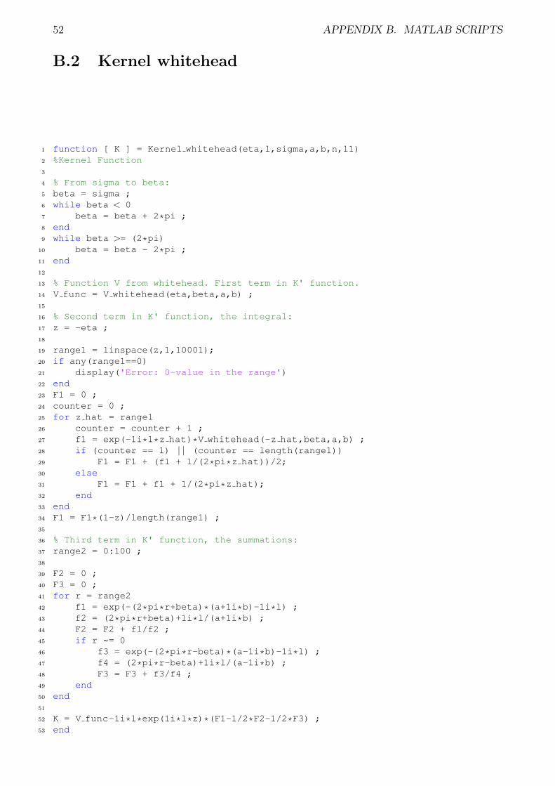
52 APPENDIX B. MATLAB SCRIPTS

B.2 Kernel whitehead

1 function [ K ] = Kernel whitehead(eta,l,sigma,a,b,n,l1)2 %Kernel Function3

4 % From sigma to beta:5 beta = sigma ;6 while beta < 07 beta = beta + 2*pi ;8 end9 while beta >= (2*pi)

10 beta = beta - 2*pi ;11 end12

13 % Function V from whitehead. First term in K' function.14 V func = V whitehead(eta,beta,a,b) ;15

16 % Second term in K' function, the integral:17 z = -eta ;18

19 range1 = linspace(z,1,10001);20 if any(range1==0)21 display('Error: 0-value in the range')22 end23 F1 = 0 ;24 counter = 0 ;25 for z hat = range126 counter = counter + 1 ;27 f1 = exp(-1i*l*z hat)*V whitehead(-z hat,beta,a,b) ;28 if (counter == 1) | | (counter == length(range1))29 F1 = F1 + (f1 + 1/(2*pi*z hat))/2;30 else31 F1 = F1 + f1 + 1/(2*pi*z hat);32 end33 end34 F1 = F1*(1-z)/length(range1) ;35

36 % Third term in K' function, the summations:37 range2 = 0:100 ;38

39 F2 = 0 ;40 F3 = 0 ;41 for r = range242 f1 = exp(-(2*pi*r+beta)*(a+1i*b)-1i*l) ;43 f2 = (2*pi*r+beta)+1i*l/(a+1i*b) ;44 F2 = F2 + f1/f2 ;45 if r ~= 046 f3 = exp(-(2*pi*r-beta)*(a-1i*b)-1i*l) ;47 f4 = (2*pi*r-beta)+1i*l/(a-1i*b) ;48 F3 = F3 + f3/f4 ;49 end50 end51

52 K = V func-1i*l*exp(1i*l*z)*(F1-1/2*F2-1/2*F3) ;53 end

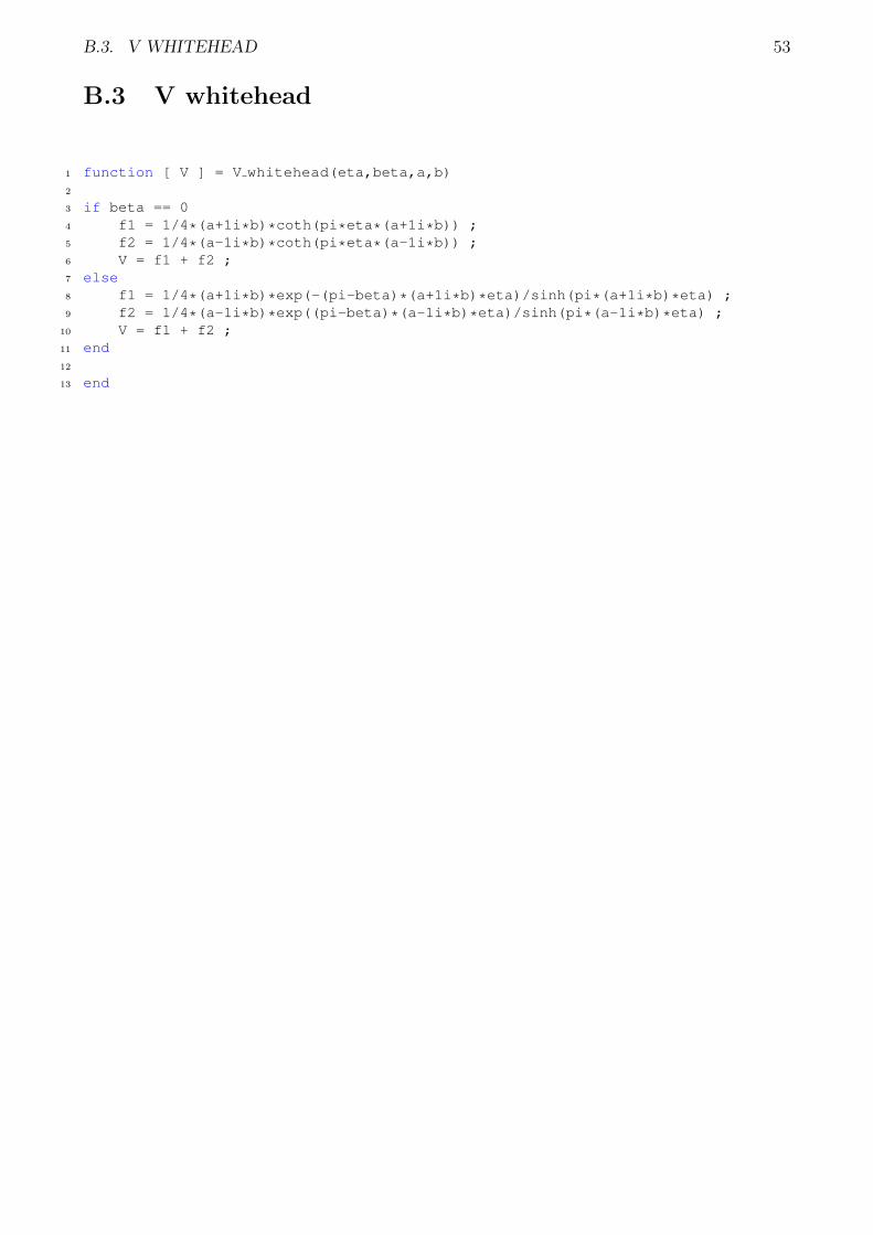
B.3. V WHITEHEAD 53

B.3 V whitehead

1 function [ V ] = V whitehead(eta,beta,a,b)2

3 if beta == 04 f1 = 1/4*(a+1i*b)*coth(pi*eta*(a+1i*b)) ;5 f2 = 1/4*(a-1i*b)*coth(pi*eta*(a-1i*b)) ;6 V = f1 + f2 ;7 else8 f1 = 1/4*(a+1i*b)*exp(-(pi-beta)*(a+1i*b)*eta)/sinh(pi*(a+1i*b)*eta) ;9 f2 = 1/4*(a-1i*b)*exp((pi-beta)*(a-1i*b)*eta)/sinh(pi*(a-1i*b)*eta) ;

10 V = f1 + f2 ;11 end12

13 end