SOUND TRACKING PAN-TILT MACHINE

Final Report for ECSE-4962

Control Systems Design

Kevin Murphy

Matthew Daigle

Matthew Gates

Vadiraj Hombal

April 28th, 2004

Rensselaer Polytechnic Institute

ii

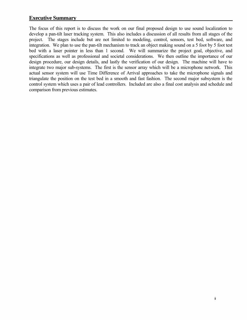
Executive Summary

The focus of this report is to discuss the work on our final proposed design to use sound localization to develop a pan-tilt laser tracking system. This also includes a discussion of all results from all stages of the project. The stages include but are not limited to modeling, control, sensors, test bed, software, and integration. We plan to use the pan-tilt mechanism to track an object making sound on a 5 foot by 5 foot test bed with a laser pointer in less than 1 second. We will summarize the project goal, objective, and specifications as well as professional and societal considerations. We then outline the importance of our design procedure, our design details, and lastly the verification of our design. The machine will have to integrate two major sub-systems. The first is the sensor array which will be a microphone network. This actual sensor system will use Time Difference of Arrival approaches to take the microphone signals and triangulate the position on the test bed in a smooth and fast fashion. The second major subsystem is the control system which uses a pair of lead controllers. Included are also a final cost analysis and schedule and comparison from previous estimates.

iii

Table of Contents

Chapter Title Page #

1 Introduction 1 2 Professional and Societal Considerations 4 3 Design Procedure 5 3.1 Modeling 5 3.2 Control System 5 3.3 Sensor System 5 3.4 System Integration 6 4 Design Details 7 4.1 Modeling 7 4.2 Control 9 4.3 Microphones 18 4.4 Time Difference of Arrival 21 4.5 Triangulation 22 4.6 System Integration 26 5 Design Verification 27 5.1 Model Validation 27 5.2 Control 28 5.3 Time Difference of Arrival and Triangulation 29 6 Costs and Schedule 33 6.1 Costs 33 6.2 Schedule 33 7 Conclusion 34 8 Bibliography 36 Appendix Title Page # A Team Member Contribution 37 B Other Experimental Results 38 C Microphone Specifications 42 D Source Code 44 E Simulink Diagrams 47 F Localization Experiment 54 G Motor, Gear, and Pulley Specifications 56

iv

List of Figures

Title Page #

Figure 1 – Block Diagram of System 1 Figure 2 – Tilt Axis Friction Plot 8 Figure 3 – Tilt Axis Step Response with Unity Gain Feedback (Linear Simulation) 11 Figure 4 - Tilt Axis Frequency Response with Unity Gain Feedback (Linear Simulation) 11 Figure 5 - Pan Axis Step Response with Unity Gain Feedback (Linear Simulation) 12 Figure 6 - Pan Axis Frequency Response with Unity Gain Feedback (Linear Simulation) 12 Figure 7 – Tilt: Frequency Response of Compensated System 14 Figure 8 – Pan: Frequency Response of Compensated System 15 Figure 9 – Tilt Axis Simulated Response to Trajectory-Generated Step 15 Figure 10 – Tilt Axis Actual Response to Trajectory-Generated Step 16 Figure 11 – Pan Axis Simulated Response to Trajectory-Generated Step 16 Figure 12 – Pan Axis Actual Response to Trajectory-Generated Step 17 Figure 13 – Velocity Filter Bode Diagram 18 Figure 14 – Input to A/D Converter 19 Figure 15 – Filtering of Microphone Signals 19 Figure 16 - Bode Diagram of Microphone Butterworth Filter 20 Figure 17 – Example of three captured microphone signals 21 Figure 18 – Signal Estimation of Max-based TDOA 22 Figure 19 - Source Triangulation in Workspace 23 Figure 20 - Effect of Sensor Perturbation on Triangulation Quantitative and Graphical View 24 Figure 21 - Degenerate Solution Caused by Sensor Perturbation 24 Figure 22 – Workspace Configuration 25 Figure 23 – Tilt Axis for +1.8 Volt 3 Second Square Pulse 27 Figure 24 - Pan Axis for +3 Volt 3 Second Pulse 28 Figure 25 - Effect of Friction Compensation 29 Figure 26 - Localization Experiment – Source Localization Error 30 Figure 27 - Effect of TDOA Perturbation on Triangulation 31 List of Tables

Title Page #

Table 1 – Tracking Specifications 2 Table 2 – Control Specifications 2 Table 3 – Identified Model Parameters 7 Table 4 – Experimentally Identified Friction Parameters 9 Table 5 – Desired and Achieved Controller Specifications 13 Table 6 - Localization Experiment 30 Table 7 – Achieved Specifications 34

1 Introduction

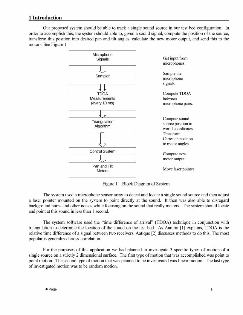
Our proposed system should be able to track a single sound source in our test bed configuration. In order to accomplish this, the system should able to, given a sound signal, compute the position of the source, transform this position into desired pan and tilt angles, calculate the new motor output, and send this to the motors. See Figure 1.

Microphone Signals Get input from

microphones.

Page

1

Figure 1 – Block Diagram of System

The system used a microphone sensor array to detect and locate a single sound source and then adjust

a laser pointer mounted on the system to point directly at the sound. It then was also able to disregard background hums and other noises while focusing on the sound that really matters. The system should locate and point at this sound in less than 1 second.

The system software used the “time difference of arrival” (TDOA) technique in conjunction with

triangulation to determine the location of the sound on the test bed. As Aarami [1] explains, TDOA is the relative time difference of a signal between two receivers. Aatique [2] discusses methods to do this. The most popular is generalized cross-correlation.

For the purposes of this application we had planned to investigate 3 specific types of motion of a

single source on a strictly 2 dimensional surface. The first type of motion that was accomplished was point to point motion. The second type of motion that was planned to be investigated was linear motion. The last type of investigated motion was to be random motion.

Sampler

Triangulation Algorithm

TDOA Measurements (every 10 ms)

Control System

Sample the microphone signals.

Compute TDOA between microphone pairs.

Compute sound source position in world coordinates. Transform Cartesian position to motor angles. Compute new motor output.

Pan and Tilt Motors Move laser pointer

Page

2

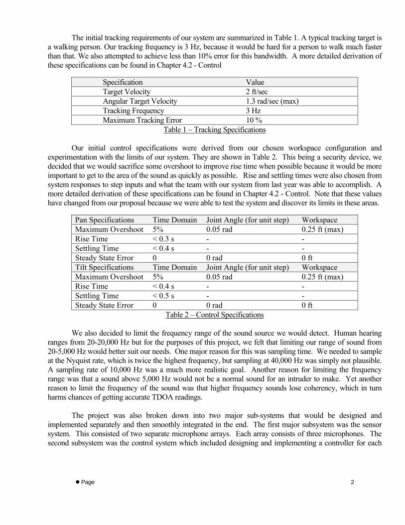
The initial tracking requirements of our system are summarized in Table 1. A typical tracking target is

a walking person. Our tracking frequency is 3 Hz, because it would be hard for a person to walk much faster than that. We also attempted to achieve less than 10% error for this bandwidth. A more detailed derivation of these specifications can be found in Chapter 4.2 - Control

Specification Value Target Velocity 2 ft/sec Angular Target Velocity 1.3 rad/sec (max) Tracking Frequency 3 Hz Maximum Tracking Error 10 %

Table 1 – Tracking Specifications

Our initial control specifications were derived from our chosen workspace configuration and experimentation with the limits of our system. They are shown in Table 2. This being a security device, we decided that we would sacrifice some overshoot to improve rise time when possible because it would be more important to get to the area of the sound as quickly as possible. Rise and settling times were also chosen from system responses to step inputs and what the team with our system from last year was able to accomplish. A more detailed derivation of these specifications can be found in Chapter 4.2 - Control. Note that these values have changed from our proposal because we were able to test the system and discover its limits in these areas.

Pan Specifications Time Domain Joint Angle (for unit step) Workspace Maximum Overshoot 5% 0.05 rad 0.25 ft (max) Rise Time < 0.3 s - - Settling Time < 0.4 s - - Steady State Error 0 0 rad 0 ft Tilt Specifications Time Domain Joint Angle (for unit step) Workspace Maximum Overshoot 5% 0.05 rad 0.25 ft (max) Rise Time < 0.4 s - - Settling Time < 0.5 s - - Steady State Error 0 0 rad 0 ft

Table 2 – Control Specifications

We also decided to limit the frequency range of the sound source we would detect. Human hearing ranges from 20-20,000 Hz but for the purposes of this project, we felt that limiting our range of sound from 20-5,000 Hz would better suit our needs. One major reason for this was sampling time. We needed to sample at the Nyquist rate, which is twice the highest frequency, but sampling at 40,000 Hz was simply not plausible. A sampling rate of 10,000 Hz was a much more realistic goal. Another reason for limiting the frequency range was that a sound above 5,000 Hz would not be a normal sound for an intruder to make. Yet another reason to limit the frequency of the sound was that higher frequency sounds lose coherency, which in turn harms chances of getting accurate TDOA readings.

The project was also broken down into two major sub-systems that would be designed and implemented separately and then smoothly integrated in the end. The first major subsystem was the sensor system. This consisted of two separate microphone arrays. Each array consists of three microphones. The second subsystem was the control system which included designing and implementing a controller for each

Page

3

axis of rotation. Also a test bed was developed, which included designing and fabricating a 5 foot by 5 foot grid on the floor and a mounting structure to hold the pan-tilt machine 5 feet above the floor.

Page

4

2 Professional and Societal Consideration

Sound detection can be an important security procedure for many applications. Whether at home, work, or elsewhere, personal protection is always one of everyone’s utmost concerns. Sound is one of several key ways to detect a security breach and being able to detect a sound in a completely dark room would enhance many current security procedures that involve video and motion detection. Our project provides for this functionality.

By designing this system we are furthering the functionality for a rather large market for security and

safety in home and safety systems worldwide. Our prospective uses and motivation are for home, work and office. The reason sound is important is because in a dark room a camera would not be good for detecting an intrusion or security breach and unlike sonar, sound based detection does not suffer from effects of specularity.

Related technology includes many other security devices such as motion/thermal detectors, security cameras, and other applications that use TDOA approaches to determine location of signals. TDOA is the current state of the art method for sound source localization. It is widely used in cell phone and satellite networks. The expected end user for a device like this would be security companies that cater to both home and business security needs. This device would be a good detection item to have and to use in conjunction with video, thermal, and/or motion sensing units.

3 Design Procedure 3.1 Modeling

The first step in system design was to model the system. Each axis was modeled as a single, decoupled joint. Due to the mounting of the pan axis and the negligible mass of our load, gravity was ignored for both axes, giving transfer functions of the form in Eqn. (1).

sBJs v+2

1 (1)

J is the total joint inertia and Bv is the viscous friction of the joint. Various parameters of the system equations were identified by parts specifications and experimentation. Once a model was found, the open loop response was simulated and compared to the actual open loop response to validate the model. This suggested the system model was accurate enough to begin control design. 3.2 Control

Control specifications were derived from the observation of system performance in the open loop, the configuration of the chosen workspace, and the expected target velocities. Lead controllers were then developed for each axis using MATLAB and rltool, converted to discrete time, and then tested in simulation. These controllers are of the following basic form shown in Eqn. (2).

)()(

pszsK

++ (2)

K is the gain, z is a zero, and p is a pole. When the nonlinear simulation gave a response that came close to or met our desired specifications, the controller was tried on the actual system to various input types. When a suitable controller was reached, the gains and amount of friction cancellation were tuned to achieve the best performance for that controller. 3.3 Sensor System

The chosen microphones are the Panasonic WM-61A omni directional back electret condenser microphone cartridges. The microphones detect frequencies in the range from 20-20,000 Hz which suited our needs for the project. We used Simulink and the A/D converter along with a simple circuit to input the signal to the target computer.

The TDOA between any two signals was estimated by examining the phase difference between two peaks. Given the estimates of TDOA between sensor pairs, computation of sound source location requires solution of the hyperbolic equations of the type in Eqn. (3).

2222 )()()()( YtYjXtXjYtYiXtXidij −+−−−+−= (3)

Page

5

The co-ordinates (Xi, Yi), (Xj, Yj) are the co-ordinates of sensors i and j respectively and (Xt, Yt) are the co-ordinates of the sound source. Previous researchers have proposed numerous methods for solution of these equations. We, however, utilized the MATLAB fsolve routine for the purpose. Apart from being the computationally most accurate solution of the system of equations, it also yields acceptable time performance. This helped us quickly settle to a method of solution and allowed us time to conduct analysis which allowed us insights into the sensor placement configuration and array and sensor pair selection for effective localization. It also allowed us to analyze the effect of perturbations of sensor positions (calibration problem) on the final achievable accuracy. Using other methods would have consumed a lot of time for the development and analysis of the method itself. 3.4 System Integration

Strict modularization and clear definition of the interfaces between these sub-systems of the entire project helped us in smooth integration of the system. The overall system samples at 0.0001 seconds. The system is first started and the microphones acquire the signal of the sound source. It is then analyzed at the host computer which returns new sound source coordinates to the target computer and hence the control system. The control system then makes the appropriate changes in the pan and tilt directions to point the laser at the sound source.

Page

6

4 Design Detail 4.1 Modeling

Modeling of the system began with the analysis of Eqn. (4).

(4)

Motor inertias and gear ratios were determined from the motor and gear specifications. The load inertias were calculated using SolidWorks. Table 3 summarizes these parameters for each joint.

Tilt Axis Parameter Symbol Identified Value Load Inertia JL 4.777x10-5 kg m2

Motor Inertia Jm 1.6x10-6 kg m2

Gear Ratio N 32.319 Pan Axis Parameter Symbol Identified Value Load Inertia JL 1.4x10-3 kg m2

Motor Inertia Jm 1.6x10-6 kg m2

Gear Ratio N 32.319

Table 3 – Identified Model Parameters

The pan axis is mounted to avoid gravity, and for the tilt axis, the load’s mass is less than 0.2 kg, therefore gravity was not identified for either joint. The gears and motors used are the same for both axes, so for both the gear ratio is described in Eqn. (5).

(2.6/0.506)*(6.3) = (5.13)*(6.3) = 32.319 (5)

The first value is the ratio of gear diameters, and the second is the motor’s internal gear ratio.

Our next step was identifying friction for each joint. This was done by first commanding a 10 volt

spike for 1 second to break static friction, then commanding constant voltage for 7 seconds. Velocities were calculated using finite differences, and steady state velocities were measured by averaging the last second of each velocity plot, for each voltage. This was done for positive and negative voltage ranges for each axis. Voltages were converted to torques using Eqn. (6)

T = (N*Kt*Kn) V (6)

where, Kt is the motor torque constant, and Kn is the current to voltage ratio for the amplifiers. This comes to 32.319*4.36x10-2*0.1 = 0.141 Nm/V. Figure 2 shows applied torque versus steady state velocity for the tilt axis. The plot for the pan axis is similar with different values for Bv and Bc. All of these values are shown in Table 4.

Page

7

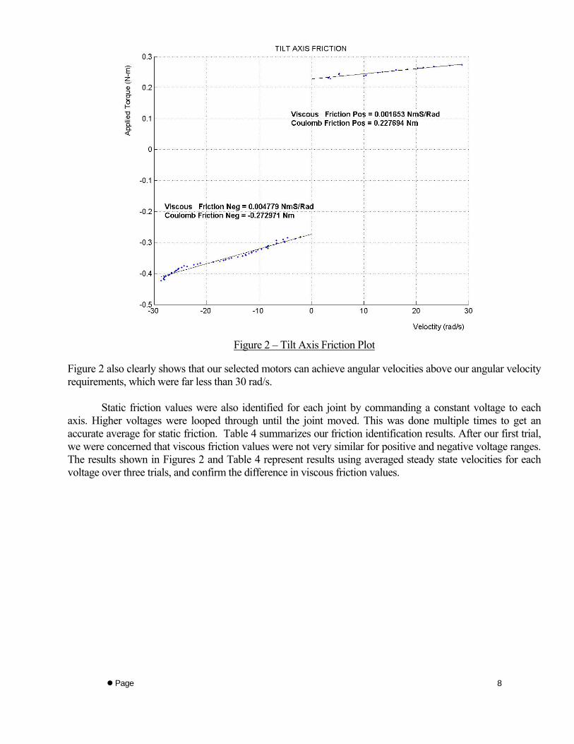
Figure 2 – Tilt Axis Friction Plot

Figure 2 also clearly shows that our selected motors can achieve angular velocities above our angular velocity requirements, which were far less than 30 rad/s.

Static friction values were also identified for each joint by commanding a constant voltage to each

axis. Higher voltages were looped through until the joint moved. This was done multiple times to get an accurate average for static friction. Table 4 summarizes our friction identification results. After our first trial, we were concerned that viscous friction values were not very similar for positive and negative voltage ranges. The results shown in Figures 2 and Table 4 represent results using averaged steady state velocities for each voltage over three trials, and confirm the difference in viscous friction values.

Page

8

Page

9

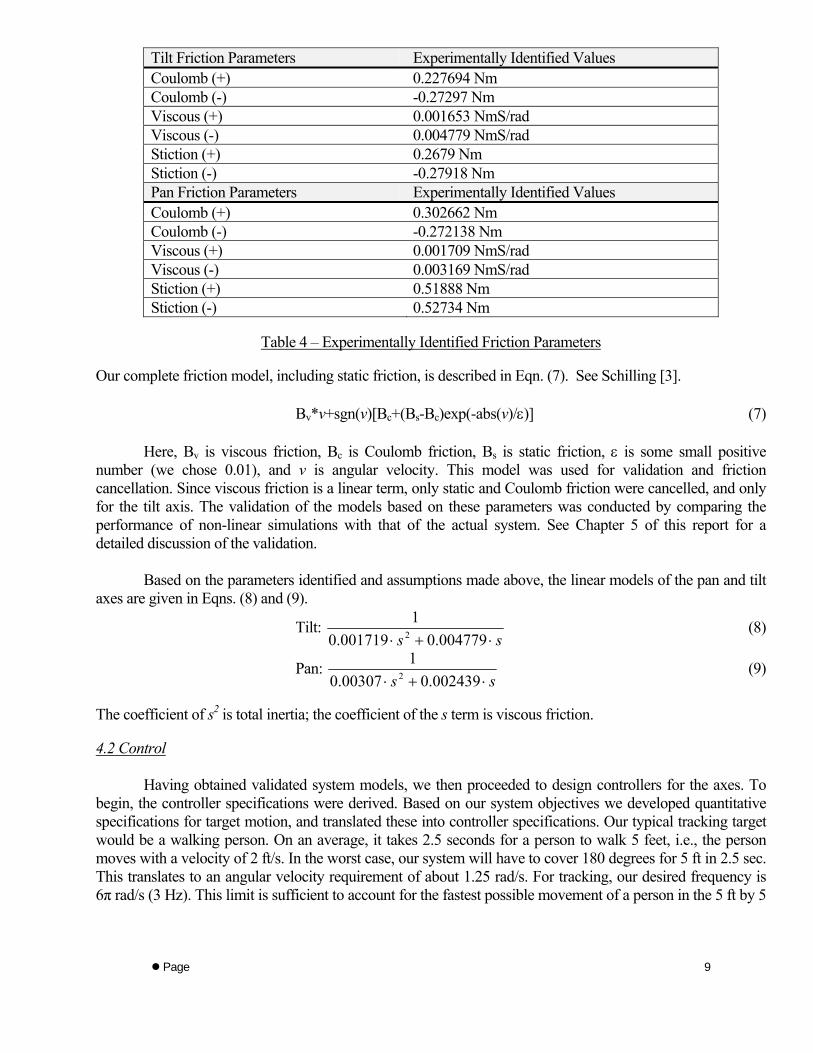
Tilt Friction Parameters Experimentally Identified Values Coulomb (+) 0.227694 Nm Coulomb (-) -0.27297 Nm Viscous (+) 0.001653 NmS/rad Viscous (-) 0.004779 NmS/rad Stiction (+) 0.2679 Nm Stiction (-) -0.27918 Nm Pan Friction Parameters Experimentally Identified Values Coulomb (+) 0.302662 Nm Coulomb (-) -0.272138 Nm Viscous (+) 0.001709 NmS/rad Viscous (-) 0.003169 NmS/rad Stiction (+) 0.51888 Nm Stiction (-) 0.52734 Nm

Table 4 – Experimentally Identified Friction Parameters

Our complete friction model, including static friction, is described in Eqn. (7). See Schilling [3].

Bv*v+sgn(v)[Bc+(Bs-Bc)exp(-abs(v)/ε)] (7)

Here, Bv is viscous friction, Bc is Coulomb friction, Bs is static friction, ε is some small positive number (we chose 0.01), and v is angular velocity. This model was used for validation and friction cancellation. Since viscous friction is a linear term, only static and Coulomb friction were cancelled, and only for the tilt axis. The validation of the models based on these parameters was conducted by comparing the performance of non-linear simulations with that of the actual system. See Chapter 5 of this report for a detailed discussion of the validation.

Based on the parameters identified and assumptions made above, the linear models of the pan and tilt

axes are given in Eqns. (8) and (9).

Tilt: ss ⋅+⋅ 004779.0001719.0

12 (8)

Pan: ss ⋅+⋅ 002439.000307.0

12 (9)

The coefficient of s2 is total inertia; the coefficient of the s term is viscous friction.

4.2 Control

Having obtained validated system models, we then proceeded to design controllers for the axes. To begin, the controller specifications were derived. Based on our system objectives we developed quantitative specifications for target motion, and translated these into controller specifications. Our typical tracking target would be a walking person. On an average, it takes 2.5 seconds for a person to walk 5 feet, i.e., the person moves with a velocity of 2 ft/s. In the worst case, our system will have to cover 180 degrees for 5 ft in 2.5 sec. This translates to an angular velocity requirement of about 1.25 rad/s. For tracking, our desired frequency is 6π rad/s (3 Hz). This limit is sufficient to account for the fastest possible movement of a person in the 5 ft by 5

Page

10

ft area that we consider. We desire to track any movement up to this frequency with less than 10% error. We consider any frequencies greater than 600π rad/s (100 Hz) as sensor or external disturbance noise in the system. In terms of open loop frequency response with controllers, these then translate to a gain requirement of at least 20 dB for frequencies up to 6π rad/s (3 Hz) and an attenuation of at least 20 dB for frequencies greater than 600π rad/s (100 Hz). The tracking requirements of our system are summarized in Table 1 of Chapter 1 - Introduction.

Our control specifications were derived from our chosen workspace configuration and experimentation with the limits of our system. Since it is important to locate an intruder quickly, we desire a relatively fast rise time and will tolerate a small amount of overshoot to achieve this. An overshoot of 5 % for either axis translates to at most 0.25 ft in our test bed. Since overshoot is only a transient property, this is acceptable. The rise and settling times were chosen from observed system responses to step inputs and our workspace limits. To cover our workspace, the worst case angular displacement limits for pan and tilt axis are 180 and 45 degrees, respectively. We require that each axis achieve these limits in less than half a second. Typically, our system will be tracking a large object, thus a small amount of steady state error is tolerable. However, we feel zero steady state error can be achieved with a decent controller. Table 2 in Chapter 1 – Introduction summarizes these specifications for each controller.

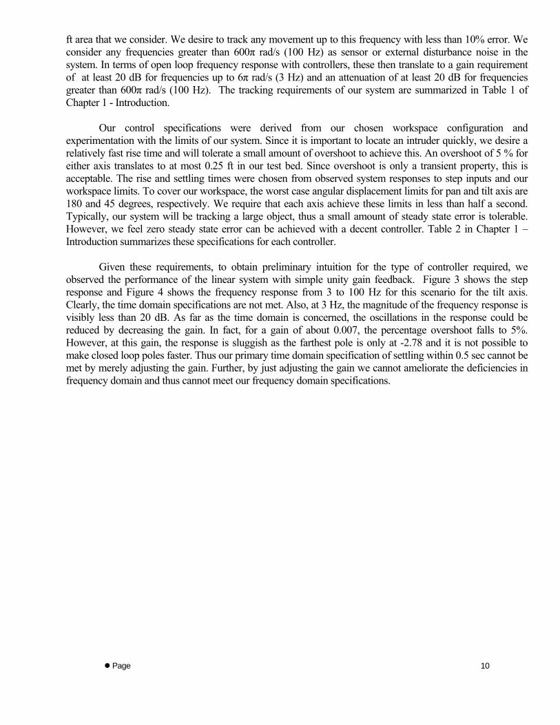
Given these requirements, to obtain preliminary intuition for the type of controller required, we observed the performance of the linear system with simple unity gain feedback. Figure 3 shows the step response and Figure 4 shows the frequency response from 3 to 100 Hz for this scenario for the tilt axis. Clearly, the time domain specifications are not met. Also, at 3 Hz, the magnitude of the frequency response is visibly less than 20 dB. As far as the time domain is concerned, the oscillations in the response could be reduced by decreasing the gain. In fact, for a gain of about 0.007, the percentage overshoot falls to 5%. However, at this gain, the response is sluggish as the farthest pole is only at -2.78 and it is not possible to make closed loop poles faster. Thus our primary time domain specification of settling within 0.5 sec cannot be met by merely adjusting the gain. Further, by just adjusting the gain we cannot ameliorate the deficiencies in frequency domain and thus cannot meet our frequency domain specifications.

Step Response

Time (sec)

Ampl

itude

0 0.5 1 1.5 2 2.5 3 3.5 40

0.2

0.4

0.6

0.8

1

1.2

1.4

1.6

1.8

2

Figure 3 – Tilt Axis Step Response with Unity Gain Feedback (Linear Simulation)

-50

-40

-30

-20

-10

0

10

Mag

nitu

de (d

B)

101

102

-180

-178

-176

-174

-172

-170

Phas

e (d

eg)

Bode Diagram - Linear Tilt Axis Model

Frequency (Hz)

Figure 4 - Tilt Axis Frequency Response with Unity Gain Feedback (Linear Simulation)

Page

11

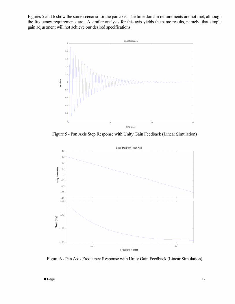
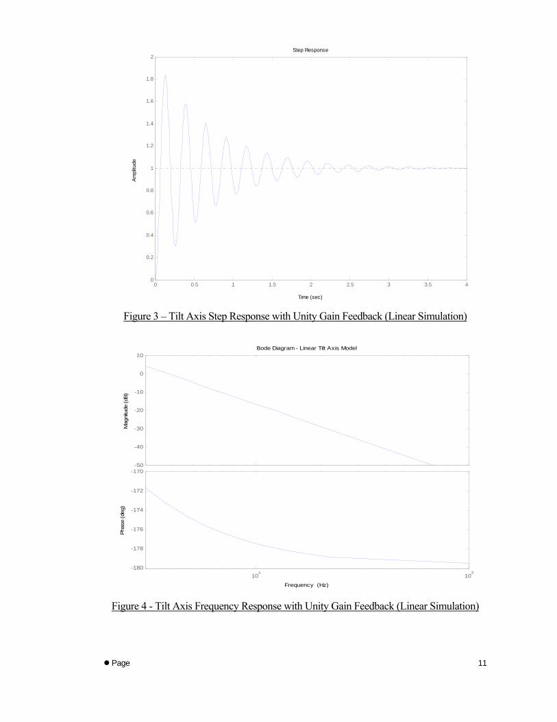
Figures 5 and 6 show the same scenario for the pan axis. The time domain requirements are not met, although the frequency requirements are. A similar analysis for this axis yields the same results, namely, that simple gain adjustment will not achieve our desired specifications.

Step Response

Time (sec)

Ampl

itude

0 5 10 150

0.2

0.4

0.6

0.8

1

1.2

1.4

1.6

1.8

2

Figure 5 - Pan Axis Step Response with Unity Gain Feedback (Linear Simulation)

-40

-30

-20

-10

0

10

20

30

40

Mag

nitu

de (d

B)

100

101

-180

-175

-170

-165

Phas

e (d

eg)

Bode Diagram - Pan Axis

Frequency (Hz)

Figure 6 - Pan Axis Frequency Response with Unity Gain Feedback (Linear Simulation)

Page

12

Clearly then, apart from damping, what is needed is an open-loop zero so that the root locus may be

pulled to the left. If properly selected, this could also have the desirable effect of introducing some lead into the system and thus compensate for the lags introduced by other subsystems in the loop. Thus both axes require compensation.

The mechanics of control design was based on transfer functions shown in Eqn. (8) for the tilt axis and

in Eqn. (9) for the pan axis and the use of MATLAB’s rltool for pole-zero placement and gain adjustment. We found that an overly aggressive controller in the linear simulation produced a desirable response in the nonlinear simulation (which more accurately represents our system). Therefore, the step responses of the linear simulations were designed to have very small rise and settling times. We also observed that unless there was a large overshoot in the linear response, the nonlinear response was sluggish. The basic design idea to achieve these characteristics was that we needed a zero as close to the origin as possible to obtain small rise and settling times. Further, a pole far in the left plane was needed to account for the increase in overshoot caused by the zero without affecting the rise and settling times. Thus a lead compensator was in order. Further, placement of the compensator zero and pole would also be constrained by our frequency domain specifications.

The controllers were designed in continuous time. Once a controller was found to yield a desirable

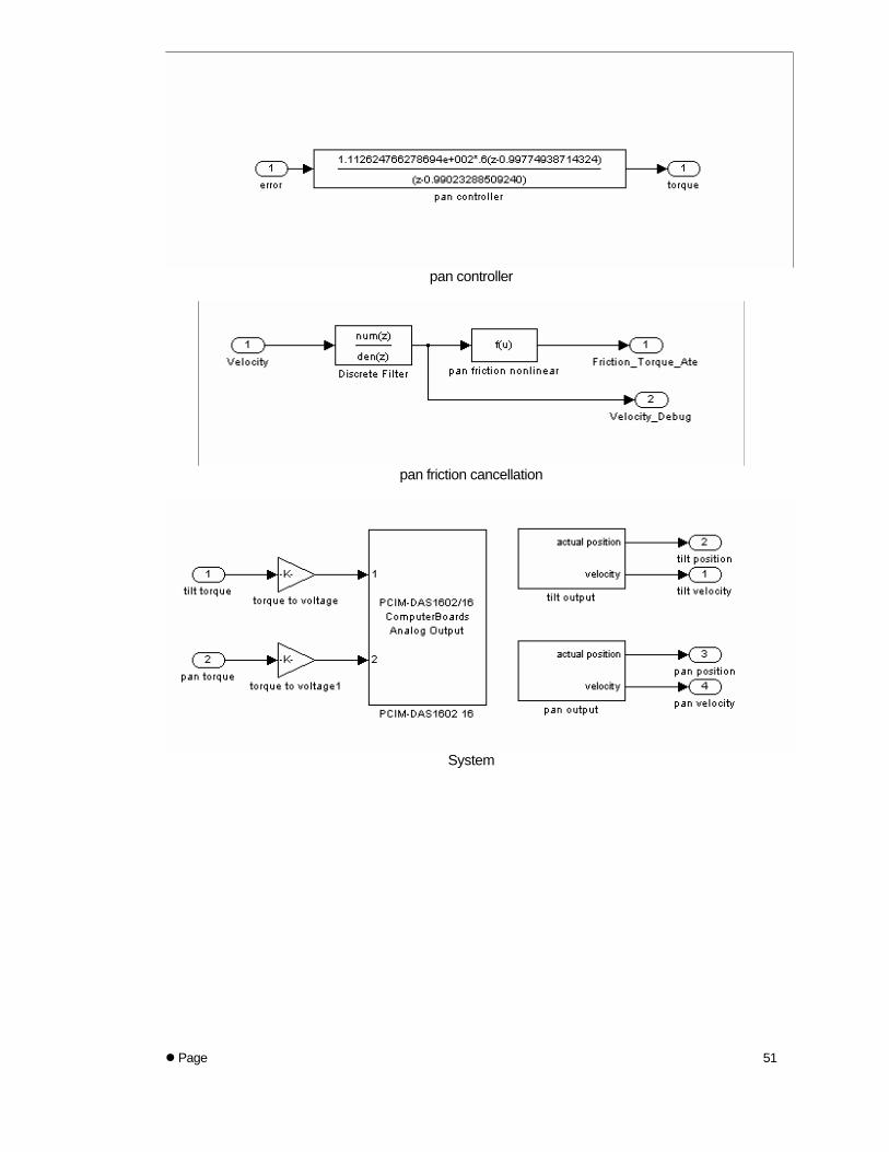
step response, a sine input was used to observe if the controller also met our tracking specifications. If so, the continuous controllers were transformed to discrete controllers with a sample time of 0.0001 seconds using the zero-order hold method. Initially, sampling of the controllers was done at 0.001 seconds, but this caused instability due to the continuous to discrete conversion of the controllers. The design process eventually produced the controllers in Eqns. (10) and (11).

Tilt: 9795.0

)99929.0(100904.1 2

−−⋅⋅

zz (10)

Pan: 990232.0

)99774.0(101126.1 2

−−⋅⋅

zz (11)

Table 5 shows the achieved specifications with these controllers.

Pan Desired Specification Achieved Specification Maximum Overshoot 5% 1% Rise Time < 0.3 s 0.15 s Settling Time < 0.4 s 0.2 s Steady State Error 0 0 (approx) Tracking < 10% at 3 Hz < 10% at 2 Hz

< 15% at 3 Hz Tilt Desired Specification Achieved Specification Maximum Overshoot 5% 0% Rise Time < 0.4 s 0.5 s Settling Time < 0.5 s 0.6 s Steady State Error 0 0 (approx) Tracking < 10% at 3 Hz < 10% at 3 Hz

Table 5 – Desired and Achieved Controller Specifications

Page

13

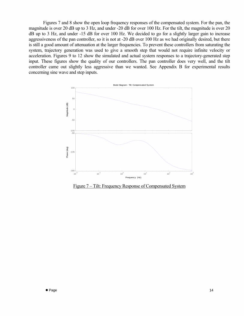
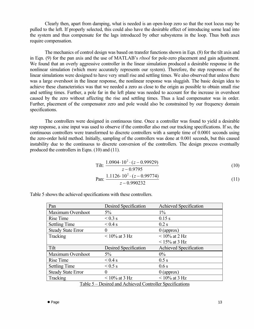
Figures 7 and 8 show the open loop frequency responses of the compensated system. For the pan, the

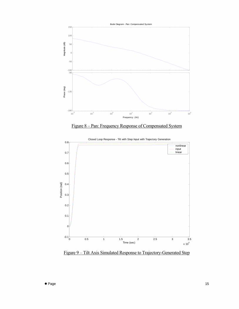
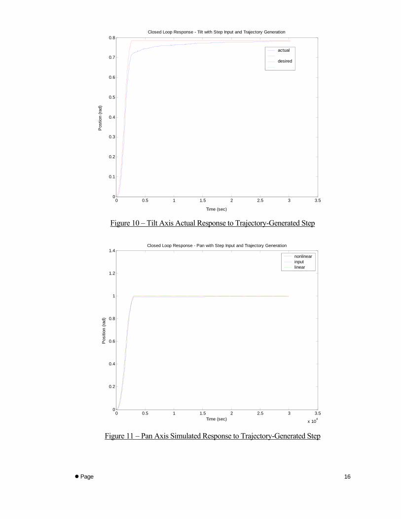
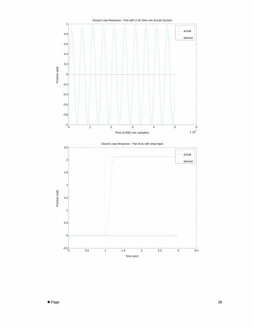
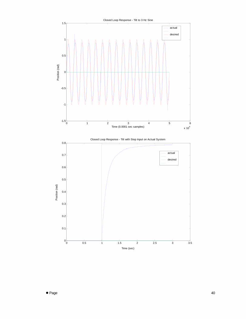
magnitude is over 20 dB up to 3 Hz, and under -20 dB for over 100 Hz. For the tilt, the magnitude is over 20 dB up to 3 Hz, and under -15 dB for over 100 Hz. We decided to go for a slightly larger gain to increase aggressiveness of the pan controller, so it is not at -20 dB over 100 Hz as we had originally desired, but there is still a good amount of attenuation at the larger frequencies. To prevent these controllers from saturating the system, trajectory generation was used to give a smooth step that would not require infinite velocity or acceleration. Figures 9 to 12 show the simulated and actual system responses to a trajectory-generated step input. These figures show the quality of our controllers. The pan controller does very well, and the tilt controller came out slightly less aggressive than we wanted. See Appendix B for experimental results concerning sine wave and step inputs.

-100

-50

0

50

100

Mag

nitu

de (d

B)

10-2

10-1

100

101

102

103

-180

-135

-90

Phas

e (d

eg)

Bode Diagram - Tilt: Compensated System

Frequency (Hz)

Figure 7 – Tilt: Frequency Response of Compensated System

Page

14

-100

-50

0

50

100

150

Mag

nitu

de (d

B)

10-2

10-1

100

101

102

103

104

-180

-135

-90

Phas

e (d

eg)

Bode Diagram - Pan: Compensated System

Frequency (Hz)

Figure 8 – Pan: Frequency Response of Compensated System

0 0.5 1 1.5 2 2.5 3 3.5

x 104

-0.1

0

0.1

0.2

0.3

0.4

0.5

0.6

0.7

0.8

Time (sec)

Pos

ition

(rad

)

Closed Loop Response - Tilt with Step Input with Trajectory Generation

nonlinearinputlinear

Figure 9 – Tilt Axis Simulated Response to Trajectory-Generated Step

Page

15

0 0.5 1 1.5 2 2.5 3 3.50

0.1

0.2

0.3

0.4

0.5

0.6

0.7

0.8

Pos

tion

(rad)

Closed Loop Response - Tilt with Step Input and Trajectory Generation

Time (sec)

actual desired

Figure 10 – Tilt Axis Actual Response to Trajectory-Generated Step

0 0.5 1 1.5 2 2.5 3 3.5

x 104

0

0.2

0.4

0.6

0.8

1

1.2

1.4

Pos

ition

(rad

)

Time (sec)

Closed Loop Response - Pan with Step Input and Trajectory Generation

nonlinearinputlinear

Figure 11 – Pan Axis Simulated Response to Trajectory-Generated Step

Page

16

0 0.5 1 1.5 2 2.5 3 3.50

0.5

1

1.5

2

2.5

3

3.5

Pos

ition

(rad

)

Closed Loop Response - Pan Axis with Step Input with Trajectory Generation

Time (sec)

actual desired

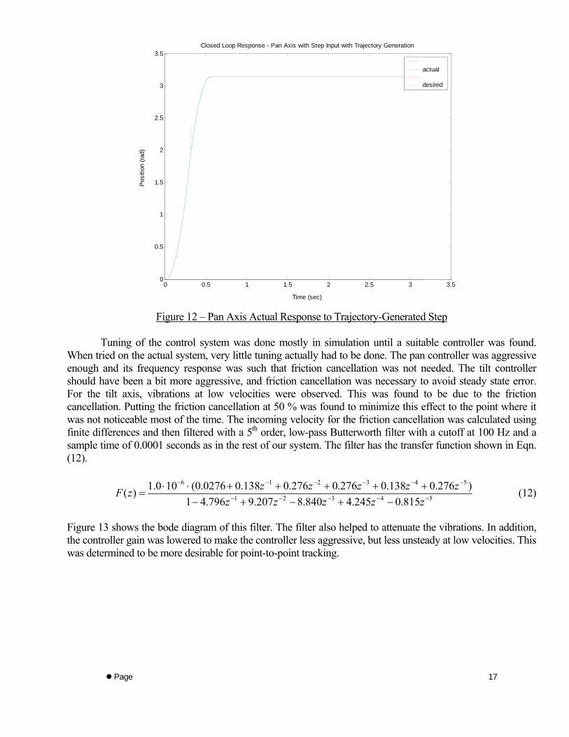
Figure 12 – Pan Axis Actual Response to Trajectory-Generated Step

Tuning of the control system was done mostly in simulation until a suitable controller was found.

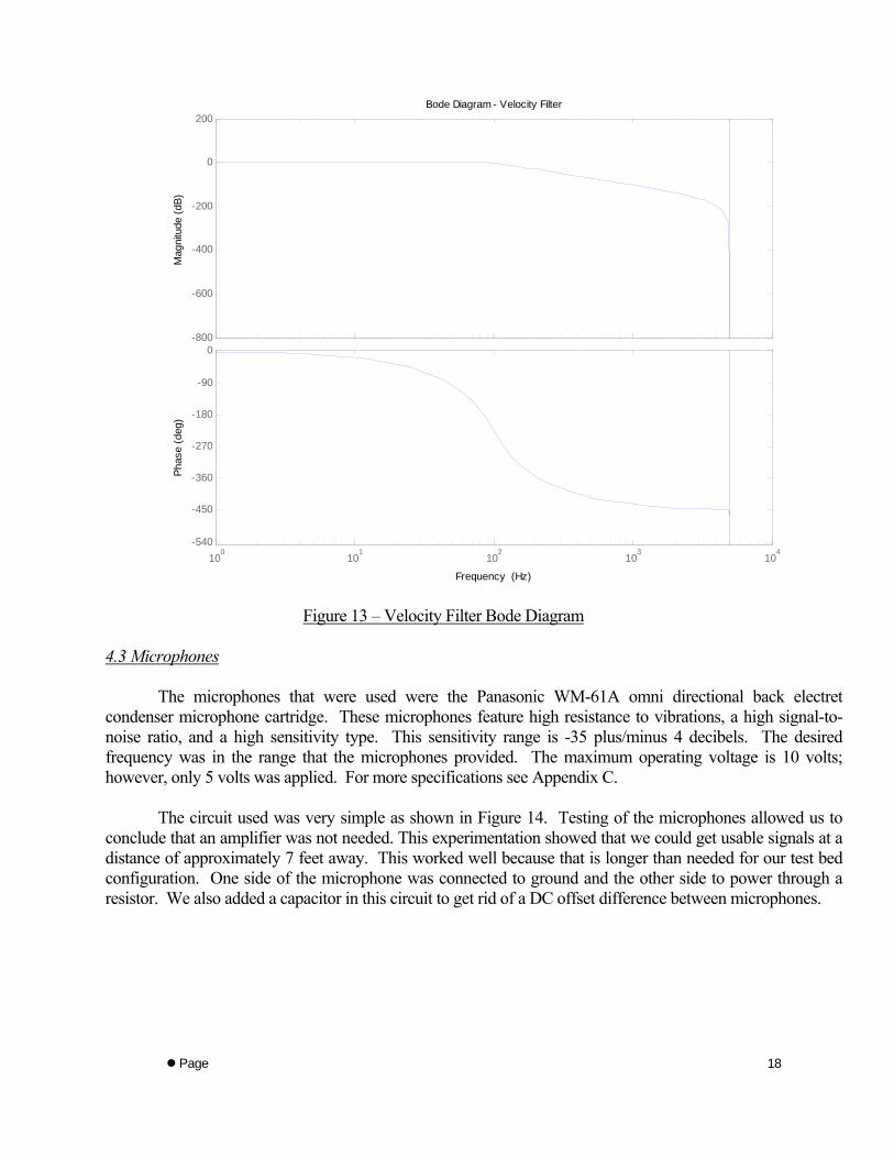
When tried on the actual system, very little tuning actually had to be done. The pan controller was aggressive enough and its frequency response was such that friction cancellation was not needed. The tilt controller should have been a bit more aggressive, and friction cancellation was necessary to avoid steady state error. For the tilt axis, vibrations at low velocities were observed. This was found to be due to the friction cancellation. Putting the friction cancellation at 50 % was found to minimize this effect to the point where it was not noticeable most of the time. The incoming velocity for the friction cancellation was calculated using finite differences and then filtered with a 5th order, low-pass Butterworth filter with a cutoff at 100 Hz and a sample time of 0.0001 seconds as in the rest of our system. The filter has the transfer function shown in Eqn. (12).

54321

543216

815.0245.4840.8207.9796.41)276.0138.0276.0276.0138.00276.0(100.1)( −−−−−

−−−−−−

−+−+−+++++⋅⋅

=zzzzz

zzzzzzF (12)

Figure 13 shows the bode diagram of this filter. The filter also helped to attenuate the vibrations. In addition, the controller gain was lowered to make the controller less aggressive, but less unsteady at low velocities. This was determined to be more desirable for point-to-point tracking.

Page

17

-800

-600

-400

-200

0

200

Mag

nitu

de (d

B)

100

101

102

103

104

-540

-450

-360

-270

-180

-90

0

Phas

e (d

eg)

Bode Diagram - Velocity Filter

Frequency (Hz)

Figure 13 – Velocity Filter Bode Diagram

4.3 Microphones

The microphones that were used were the Panasonic WM-61A omni directional back electret condenser microphone cartridge. These microphones feature high resistance to vibrations, a high signal-to-noise ratio, and a high sensitivity type. This sensitivity range is -35 plus/minus 4 decibels. The desired frequency was in the range that the microphones provided. The maximum operating voltage is 10 volts; however, only 5 volts was applied. For more specifications see Appendix C.

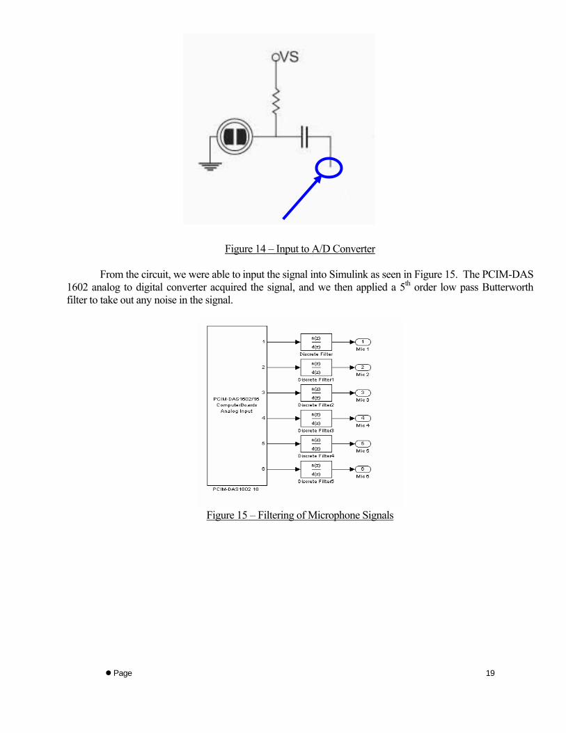
The circuit used was very simple as shown in Figure 14. Testing of the microphones allowed us to

conclude that an amplifier was not needed. This experimentation showed that we could get usable signals at a distance of approximately 7 feet away. This worked well because that is longer than needed for our test bed configuration. One side of the microphone was connected to ground and the other side to power through a resistor. We also added a capacitor in this circuit to get rid of a DC offset difference between microphones.

Page

18

Page

19

Figure 14 – Input to A/D Converter

From the circuit, we were able to input the signal into Simulink as seen in Figure 15. The PCIM-DAS

1602 analog to digital converter acquired the signal, and we then applied a 5th order low pass Butterworth filter to take out any noise in the signal.

Figure 15 – Filtering of Microphone Signals

-300

-200

-100

0

100

Mag

nitu

de (d

B)

102

103

104

-720

-540

-360

-180

0

Phas

e (d

eg)

Bode DiagramGm = 0.748 dB (at 3.83e+003 Hz) , Pm = 169 deg (at 564 Hz)

Frequency (Hz)

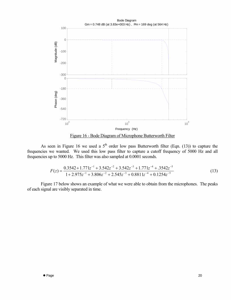
Figure 16 - Bode Diagram of Microphone Butterworth Filter

As seen in Figure 16 we used a 5th order low pass Butterworth filter (Eqn. (13)) to capture the frequencies we wanted. We used this low pass filter to capture a cutoff frequency of 5000 Hz and all frequencies up to 5000 Hz. This filter was also sampled at 0.0001 seconds.

54321

54321

1254.08811.0545.2806.3975.213542.771.1542.3542.3771.13542.0)(

−−−−−

−−−−−

++++++++++

=zzzzz

zzzzzzF (13)

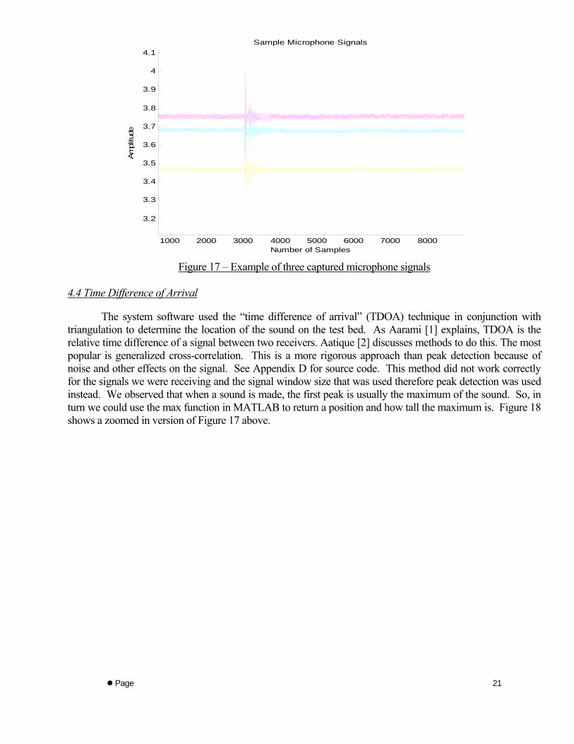
Figure 17 below shows an example of what we were able to obtain from the microphones. The peaks

of each signal are visibly separated in time.

Page

20

1000 2000 3000 4000 5000 6000 7000 8000

3.2

3.3

3.4

3.5

3.6

3.7

3.8

3.9

4

4.1

Number of Samples

Am

plitu

de

Sample Microphone Signals

Figure 17 – Example of three captured microphone signals

4.4 Time Difference of Arrival

The system software used the “time difference of arrival” (TDOA) technique in conjunction with

triangulation to determine the location of the sound on the test bed. As Aarami [1] explains, TDOA is the relative time difference of a signal between two receivers. Aatique [2] discusses methods to do this. The most popular is generalized cross-correlation. This is a more rigorous approach than peak detection because of noise and other effects on the signal. See Appendix D for source code. This method did not work correctly for the signals we were receiving and the signal window size that was used therefore peak detection was used instead. We observed that when a sound is made, the first peak is usually the maximum of the sound. So, in turn we could use the max function in MATLAB to return a position and how tall the maximum is. Figure 18 shows a zoomed in version of Figure 17 above.

Page

21

Microphones

Signal Maximums

Figure 18 – Signal Estimation of Max-based TDOA

We then subtracted the times and multiplied by our sampling frequency. If the TDOA was negative then signal 2 leads signal 1, and if it was positive signal 1 leads signal 2. After computing this we sent it to our triangulation script. To determine which sensor array to use we added the signals together on their respective sides. We then used the side with the smaller signal strength. If we used the signals from the side where the source originated then there could be degenerative solutions. See Appendix D for source code that was used. This was a simplified method but then again not as precise as cross correlation would be. Cross correlation would be absolutely needed when the sound source is not a clearly distinguishable sound or when amplitude variations arise due to noise.

4.5 Triangulation

If we let Tij be the TDOA of sound signals emitted from the source, located at (Xt,Yt), and received at sensors i and j located at (Xi,Yi) and (Xj,Yj) respectively. Sa is the speed of sound in air (1134 ft/s at 74 degree Fahrenheit). The distance difference of the sound source to sensors is then given by Eqn. (14).

2222 )()()()( YtYjXtXjYtYiXtXiTijSadij −+−−−+−=×= (14)

Thus, given the TDOA between sensor pairs, source localization is the problem of finding solutions of the hyperbolic equations of the above type. Clearly, we need a minimum of two such equations r presenthe dist

e ting ances differences of the source from 3 sensors, to determine the position of the source. In general, two

hyperbolas intersect at 0, 1 or 2 points. In terms of sound source triangulation these correspond to degenerate, desired and un-observable source conditions. Exploration of situations leading to these conditions provides us with insights in to the design of sensor configuration and selection.

Page

22

Page

23

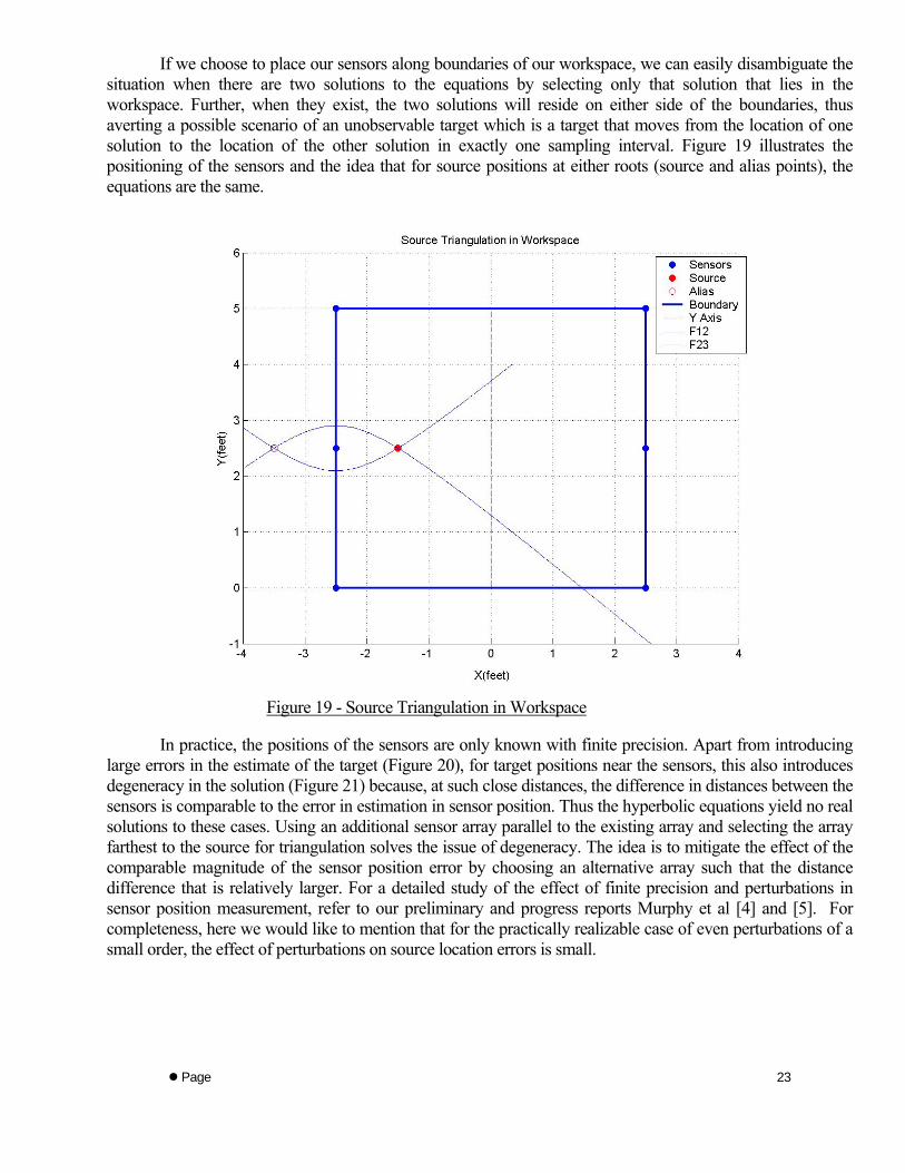
cting only that solution that lies in the workspace. Further, when they exist, the two solutions will reside on either side of the boundaries, thus averting

If we choose to place our sensors along boundaries of our workspace, we can easily disambiguate the situation when there are two solutions to the equations by sele

a possible scenario of an unobservable target which is a target that moves from the location of one solution to the location of the other solution in exactly one sampling interval. Figure 19 illustrates the positioning of the sensors and the idea that for source positions at either roots (source and alias points), the equations are the same.

Figure 19 - Source Triangulation in Workspace

In practice, the positions of the sensors are only known with finite precision. Apart from introducing large errors in the estim near the sensors, this also introduces degeneracy in the solution (Figure 21) because, at such close distances, the difference in distances between the sensors

ate of the target (Figure 20), for target positions

is comparable to the error in estimation in sensor position. Thus the hyperbolic equations yield no real solutions to these cases. Using an additional sensor array parallel to the existing array and selecting the array farthest to the source for triangulation solves the issue of degeneracy. The idea is to mitigate the effect of the comparable magnitude of the sensor position error by choosing an alternative array such that the distance difference that is relatively larger. For a detailed study of the effect of finite precision and perturbations in sensor position measurement, refer to our preliminary and progress reports Murphy et al [4] and [5]. For completeness, here we would like to mention that for the practically realizable case of even perturbations of a small order, the effect of perturbations on source location errors is small.

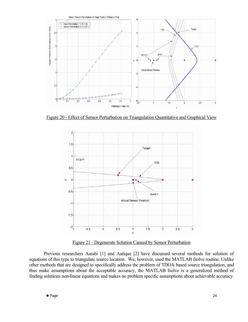
Figure 20 - Effect of Sensor Perturbation on Triangulation Quantitative and Graphical View

Figure 21 - Degenerate Solution Caused by Sensor Perturbation

Previous researchers Aarabi [1] and Aatique [2] have discussed several methods for solution of equations of this type to triangulate source location. We, however, used the MATLAB fsolve routine. Unlike other methods that are designed to specifically address the problem of TDOA based source triangulation, and thus make assumptions about the acceptable accuracy, the MATLAB fsolve is a generalized method of finding solutions non-linear equations and makes no problem specific assumptions about achievable accuracy.

Page

24

Further, use of a well established method frees us from the necessity to validate, develop and test the methodology itself.

The mean runtime (over several runs) for fsolve based triangulation using two equations was found to

be 0.02s on a 2.7 G Hz Pentium 4 machine and 0.18s on a Pentium 3 running at 498 M Hz with 128 MB RAM. Further, these estimates increase as the number of equations (over-determined system) increases. Because we established that the two contingencies, degenerate and unobservable target conditions, could be resolved through careful positioning and selection of sensor arrays, over-determined systems do not provide any real benefits. Thus, 2 arrays, with 3 sensors in each, are sufficient for source triangulation. Appendix D lists all pertinent source code. 4.6 System Integration

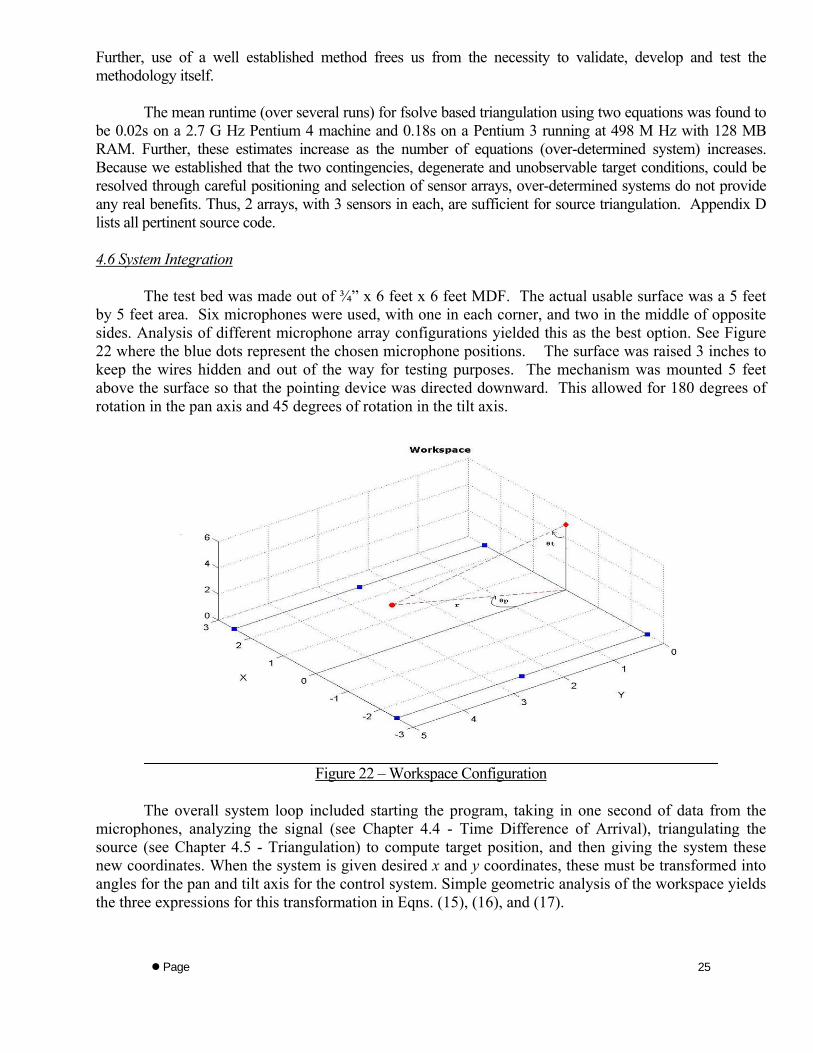
The test bed was made out of ¾” x 6 feet x 6 feet MDF. The actual usable surface was a 5 feet by 5 feet area. Six microphones were used, with one in each corner, and two in the middle of opposite sides. Analysis of different microphone array configurations yielded this as the best option. See Figure 22 where the blue dots represent the chosen microphone positions. The surface was raised 3 inches to keep the wires hidden and out of the way for testing purposes. The mechanism was mounted 5 feet above the surface so that the pointing device was directed downward. This allowed for 180 degrees of rotation in the pan axis and 45 degrees of rotation in the tilt axis.

Figure 22 – Workspace Configuration

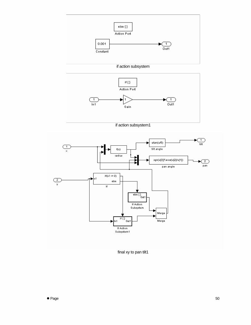
The overall system loop included starting the program, taking in one second of data from the microphones, analyzing the signal (see Chapter 4.4 - Time Difference of Arrival), triangulating the source (see Chapter 4.5 - Triangulation) to compute target position, and then giving the system these new coordinates. When the system is given desired x and y coordinates, these must be transformed into angles for the pan and tilt axis for the control system. Simple geometric analysis of the workspace yields the three expressions for this transformation in Eqns. (15), (16), and (17).

Page

25

22 yxr += (15)

)/(cos 1 ryp−=θ (16)

)5/(tan 1 rt−=θ (17)

One issue that the system also dealt with was the case when r was zero, which causes the cos-1 function to give an infinite angle instead of just zero. A simple if statement in the Simulink diagram checked for this problem and accounted for it by setting y to 0.0001. Figure 22 also shows the workspace and the convention used for θp and θt. The upper red dot represents the location of our pointing device, and the lower red dot represents an arbitrary target position.

In a production application of our system, the loop would consist of continuously running the system, and every 100 samples, computing the TDOAs, inputting them into a lookup table or triangulating with an fsolve s-function interface to get target position, and then setting the new position. The lookup table would be pre-calculated for the chosen workspace configuration.

Page

26

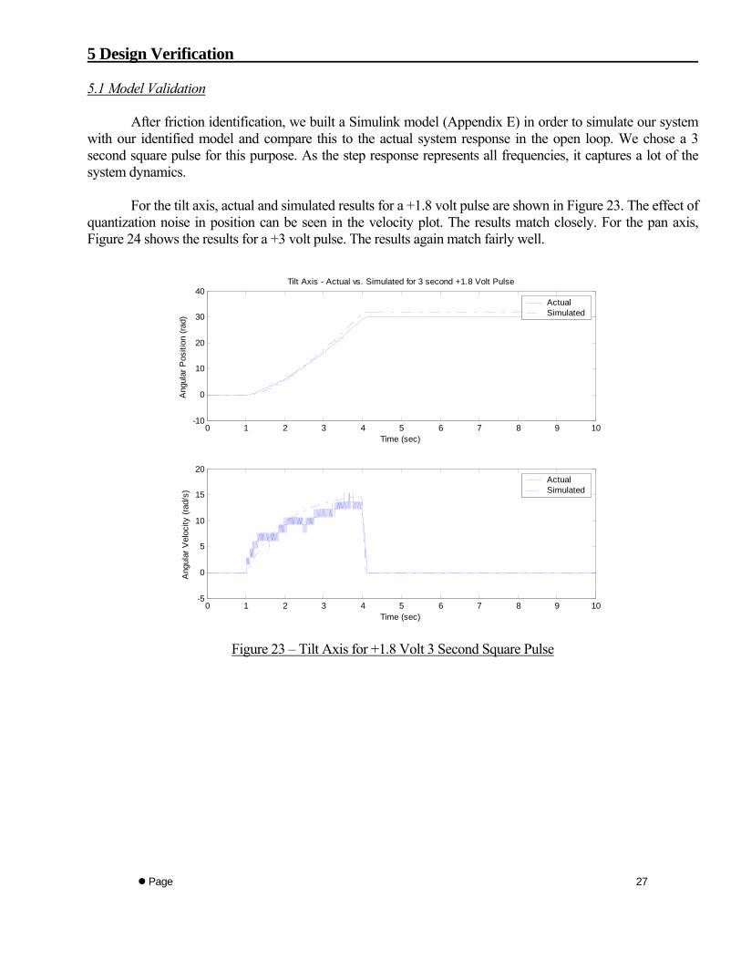
5 Design Verification 5.1 Model Validation

After friction identification, we built a Simulink model (Appendix E) in order to simulate our system with our identified model and compare this to the actual system response in the open loop. We chose a 3 second square pulse for this purpose. As the step response represents all frequencies, it captures a lot of the system dynamics.

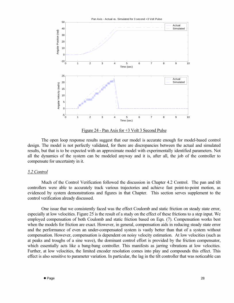
For the tilt axis, actual and simulated results for a +1.8 volt pulse are shown in Figure 23. The effect of quantization noise in position can be seen in the velocity plot. The results match closely. For the pan axis, Figure 24 shows the results for a +3 volt pulse. The results again match fairly well.

0 1 2 3 4 5 6 7 8 9 10-10

0

10

20

30

40

Time (sec)

Ang

ular

Pos

ition

(rad

)

Tilt Axis - Actual vs. Simulated for 3 second +1.8 Volt Pulse

ActualSimulated

0 1 2 3 4 5 6 7 8 9 10-5

0

5

10

15

20

Time (sec)

Ang

ular

Vel

ocity

(rad

/s)

ActualSimulated

Figure 23 – Tilt Axis for +1.8 Volt 3 Second Square Pulse

Page

27

0 1 2 3 4 5 6 7 8 9 10-10

0

10

20

30

40

50

Time (sec)

Ang

ular

Pos

ition

(rad

)

Pan Axis - Actual vs. Simulated for 3 second +3 Volt Pulse

ActualSimulated

0 1 2 3 4 5 6 7 8 9 10-5

0

5

10

15

20

25

Time (sec)

Ang

ular

Vel

ocity

(rad

/s)

ActualSimulated

Figure 24 - Pan Axis for +3 Volt 3 Second Pulse

The open loop response results suggest that our model is accurate enough for model-based control

design. The model is not perfectly validated, for there are discrepancies between the actual and simulated results, but that is to be expected with an approximate model with experimentally identified parameters. Not all the dynamics of the system can be modeled anyway and it is, after all, the job of the controller to compensate for uncertainty in it. 5.2 Control

Much of the Control Verification followed the discussion in Chapter 4.2 Control. The pan and tilt controllers were able to accurately track various trajectories and achieve fast point-to-point motion, as evidenced by system demonstrations and figures in that Chapter. This section serves supplement to the control verification already discussed.

One issue that we consistently faced was the effect Coulomb and static friction on steady state error,

especially at low velocities. Figure 25 is the result of a study on the effect of these frictions to a step input. We employed compensation of both Coulomb and static friction based on Eqn. (7). Compensation works best when the models for friction are exact. However, in general, compensation aids in reducing steady state error and the performance of even an under-compensated system is vastly better than that of a system without compensation. However, compensation is dependent on noisy velocity estimation. At low velocities (such as at peaks and troughs of a sine wave), the dominant control effort is provided by the friction compensator, which essentially acts like a bang-bang controller. This manifests as jarring vibrations at low velocities. Further, at low velocities, the limited encoder resolution comes into play and compounds this effect. This effect is also sensitive to parameter variation. In particular, the lag in the tilt controller that was noticeable can

Page

28

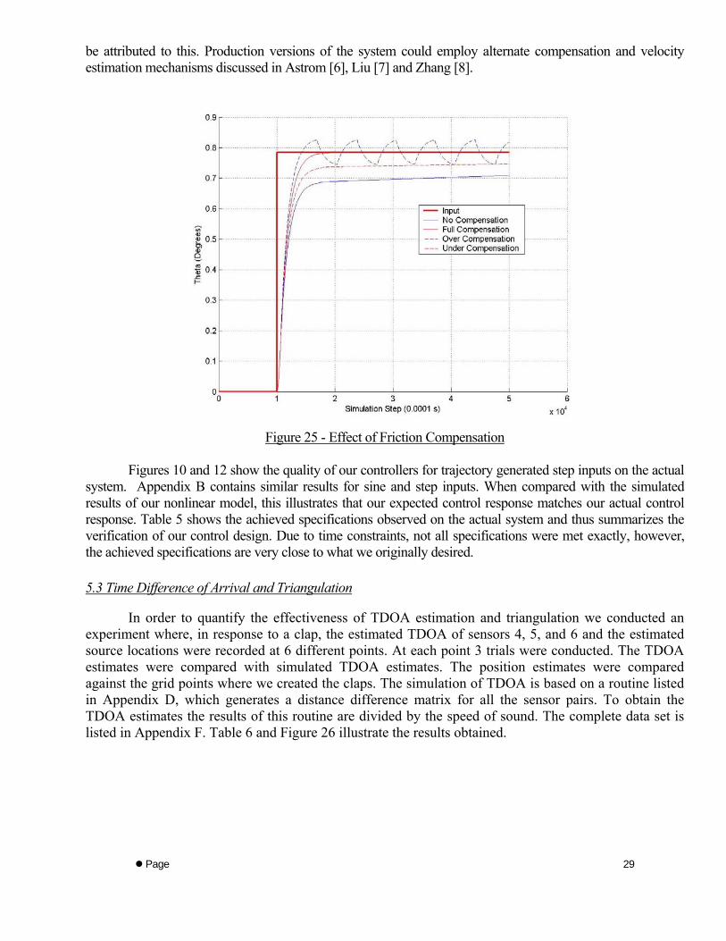
be attributed to this. Production versions of the system could employ alternate compensation and velocity estimation mechanisms discussed in Astrom [6], Liu [7] and Zhang [8].

Figure 25 - Effect of Friction Compensation

Figures 10 and 12 show the quality of our controllers for trajectory generated step inputs on the actual

system. Appendix B contains similar results for sine and step inputs. When compared with the simulated results of our nonlinear model, this illustrates that our expected control response matches our actual control response. Table 5 shows the achieved specifications observed on the actual system and thus summarizes the verification of our control design. Due to time constraints, not all specifications were met exactly, however, the achieved specifications are very close to what we originally desired. 5.3 Time Difference of Arrival and Triangulation

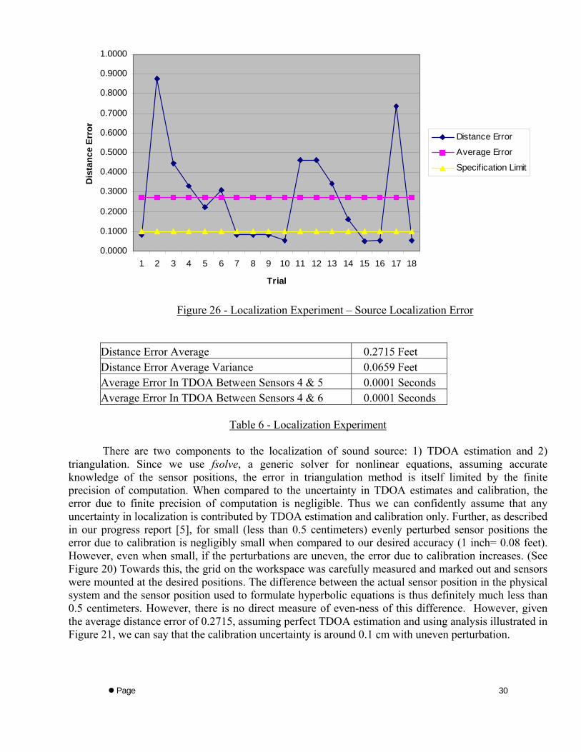
In order to quantify the effectiveness of TDOA estimation and triangulation we conducted an experiment where, in response to a clap, the estimated TDOA of sensors 4, 5, and 6 and the estimated source locations were recorded at 6 different points. At each point 3 trials were conducted. The TDOA estimates were compared with simulated TDOA estimates. The position estimates were compared against the grid points where we created the claps. The simulation of TDOA is based on a routine listed in Appendix D, which generates a distance difference matrix for all the sensor pairs. To obtain the TDOA estimates the results of this routine are divided by the speed of sound. The complete data set is listed in Appendix F. Table 6 and Figure 26 illustrate the results obtained.

Page

29

0.0000

0.1000

0.2000

0.3000

0.4000

0.5000

0.6000

0.7000

0.8000

0.9000

1.0000

1 2 3 4 5 6 7 8 9 10 11 12 13 14 15 16 17 18

Trial

Dis

tanc

e Er

ror

Distance Error

Average Error

Specif ication Limit

Figure 26 - Localization Experiment – Source Localization Error

Distance Error Average 0.2715 Feet Distance Error Average Variance 0.0659 Feet Average Error In TDOA Between Sensors 4 & 5 0.0001 Seconds Average Error In TDOA Between Sensors 4 & 6 0.0001 Seconds

Table 6 - Localization Experiment

There are two components to the localization of sound source: 1) TDOA estimation and 2)

triangulation. Since we use fsolve, a generic solver for nonlinear equations, assuming accurate knowledge of the sensor positions, the error in triangulation method is itself limited by the finite precision of computation. When compared to the uncertainty in TDOA estimates and calibration, the error due to finite precision of computation is negligible. Thus we can confidently assume that any uncertainty in localization is contributed by TDOA estimation and calibration only. Further, as described in our progress report [5], for small (less than 0.5 centimeters) evenly perturbed sensor positions the error due to calibration is negligibly small when compared to our desired accuracy (1 inch= 0.08 feet). However, even when small, if the perturbations are uneven, the error due to calibration increases. (See Figure 20) Towards this, the grid on the workspace was carefully measured and marked out and sensors were mounted at the desired positions. The difference between the actual sensor position in the physical system and the sensor position used to formulate hyperbolic equations is thus definitely much less than 0.5 centimeters. However, there is no direct measure of even-ness of this difference. However, given the average distance error of 0.2715, assuming perfect TDOA estimation and using analysis illustrated in Figure 21, we can say that the calibration uncertainty is around 0.1 cm with uneven perturbation.

Page

30

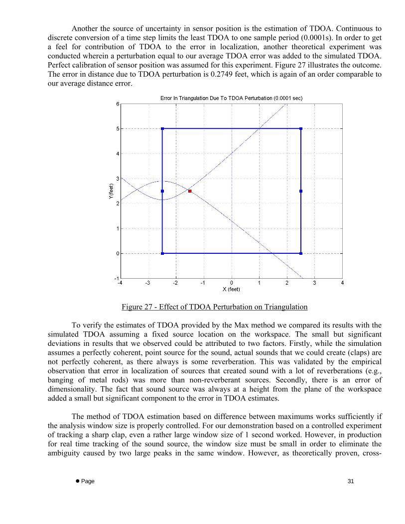
Another the source of uncertainty in sensor position is the estimation of TDOA. Continuous to discrete conversion of a time step limits the least TDOA to one sample period (0.0001s). In order to get a feel for contribution of TDOA to the error in localization, another theoretical experiment was conducted wherein a perturbation equal to our average TDOA error was added to the simulated TDOA. Perfect calibration of sensor position was assumed for this experiment. Figure 27 illustrates the outcome. The error in distance due to TDOA perturbation is 0.2749 feet, which is again of an order comparable to our average distance error.

Figure 27 - Effect of TDOA Perturbation on Triangulation

To verify the estimates of TDOA provided by the Max method we compared its results with the

simulated TDOA assuming a fixed source location on the workspace. The small but significant deviations in results that we observed could be attributed to two factors. Firstly, while the simulation assumes a perfectly coherent, point source for the sound, actual sounds that we could create (claps) are not perfectly coherent, as there always is some reverberation. This was validated by the empirical observation that error in localization of sources that created sound with a lot of reverberations (e.g., banging of metal rods) was more than non-reverberant sources. Secondly, there is an error of dimensionality. The fact that sound source was always at a height from the plane of the workspace added a small but significant component to the error in TDOA estimates.

The method of TDOA estimation based on difference between maximums works sufficiently if the analysis window size is properly controlled. For our demonstration based on a controlled experiment of tracking a sharp clap, even a rather large window size of 1 second worked. However, in production for real time tracking of the sound source, the window size must be small in order to eliminate the ambiguity caused by two large peaks in the same window. However, as theoretically proven, cross-

Page

31

Page

32

correlation as a method is much more superior (offering noise rejection) and further research into exploring this option must be conducted before production.

Detailed analysis of the triangulation method provided us with important results that we used to implement the solution. Specifically, the sensor configuration and array selection algorithm were based on theoretical study. As a consequence, we observed neither degeneracy nor blind zones in the triangulation of the sound source in the workspace.

Apart from signal processing and control issues described above, the system faces some

mechanical issues too. The error in alignment of the pan-tilt unit about the origin was caused due a slight slant in the alignment of the support structure of our test bed, the errors in physically mounting the pan-tilt unit at the origin and the alignment of the laser pointer with respect to the tilt-axis. However, this is a static type of error and was corrected by manually adjusting the setup. In production, this could be remedied with precise construction of the support structure and laser pointer and also with calibrated mounting.

A more important mechanical source of disturbance is the vibration of the support structure when the pan-tilt unit is running. The errors due to vibrations accumulate and cause the position of the pan-tilt unit to shift. This effect manifests in several ways including creation of a visually jarring effect of the laser trace on the workspace to a shift of origin of the pan-tilt unit due to slippage. It also adds to the effects of coupling between the two motors. In severe cases it could also lead to deviations in encoder readings. However, as our pan-tilt unit was smooth and the support structure relatively rigid, the effect of vibrations though palpable was not considerable. Again, in production, creating a more rigid support structure can reduce the effect of this uncertainty.

We tested our system in the fairly noisy environs of an end-of-the-semester-lab that was shared by students of two classes. This environment can be considered as a worst-case scenario as, a rather silent environment, disturbed only by the sounds of an intruder, would surround any production system used in security environments. On an average we observed the localization of the sound source was within 0.25 feet (3 inches) of position of the clap. Even though this is greater than our initial aggressive specification, given our testing environment and various sources of uncertainty discussed above, this result validates the concept of sound based tracking. The media clips on the Final Report CD show the acquisition of a sound source and thus visually establish the proof of concept for sound-based tracking.

Page

33

6 Costs and Schedule Analysis 6.1 Costs We have compared our actual costs from the estimated one from our project proposal. Our estimated new cost was $83.50. We were subsequently informed that we would be allowed a $100 budget for the project. We have now computed all relevant costs during the semester. Below is a list of the new parts and cost to date as well as a list of overall project cost.

New Parts: Price MDF Board (x2) $37.92 2”x 3” Wood (x3) $ 3.99 2”x 4” Wood (x3) $ 7.32 Wood Screws $ 3.65 6’ Computer Cable Extender $13.99 Electronic Circuit Supplies $22.60 Microphone Cartridges (x10) $16.21 Subtotal (Final) $105.68 Estimated cost from Proposal $ 83.50 Budgeted Constraint $100.00 Amount Over Budget $ 5.68 6.2 Schedule We have compared our actual schedule to that of our project proposal. Below is the schedule from that proposal. We believe it was a good outline for our work throughout the semester. We were on schedule most of the time. We do believe, looking back, that it would have been better for us if we had allotted more time for signal analysis as well as system integration. Having additional time for each of those tasks would have allowed us to better complete and enhance our project. Week Task(s) Persons 6 (2/15 – 2/21) Final Design and Modeling Hombal 7 (2/22 – 2/28) Order Parts Gates Verification of Model Daigle / Hombal 8 (2/29 – 3/6) Pan/Tilt System Construction Gates MATLAB algorithms for TDOA Hombal / Daigle 9(3/7 – 3/13) SPRINK BREAK 10 (3/14 – 3/20) Work on Progress Report/Presentation Team 11 (3/21 – 3/27) Control System (PID) Construction Murphy / Gates 12 (3/28 – 4/3) Sensor Network Construction Murphy / Gates 13 (4/4 – 4/10) System Integration Team (Control System and Sensors) 14 (4/11 – 4/17) Final Tuning and Optimization Team Final System Demonstration Team 15 (4/18 – 4/24) Final System Presentation Team 16 (4/25 – 4/28) Work on Final Report Team

Page

34

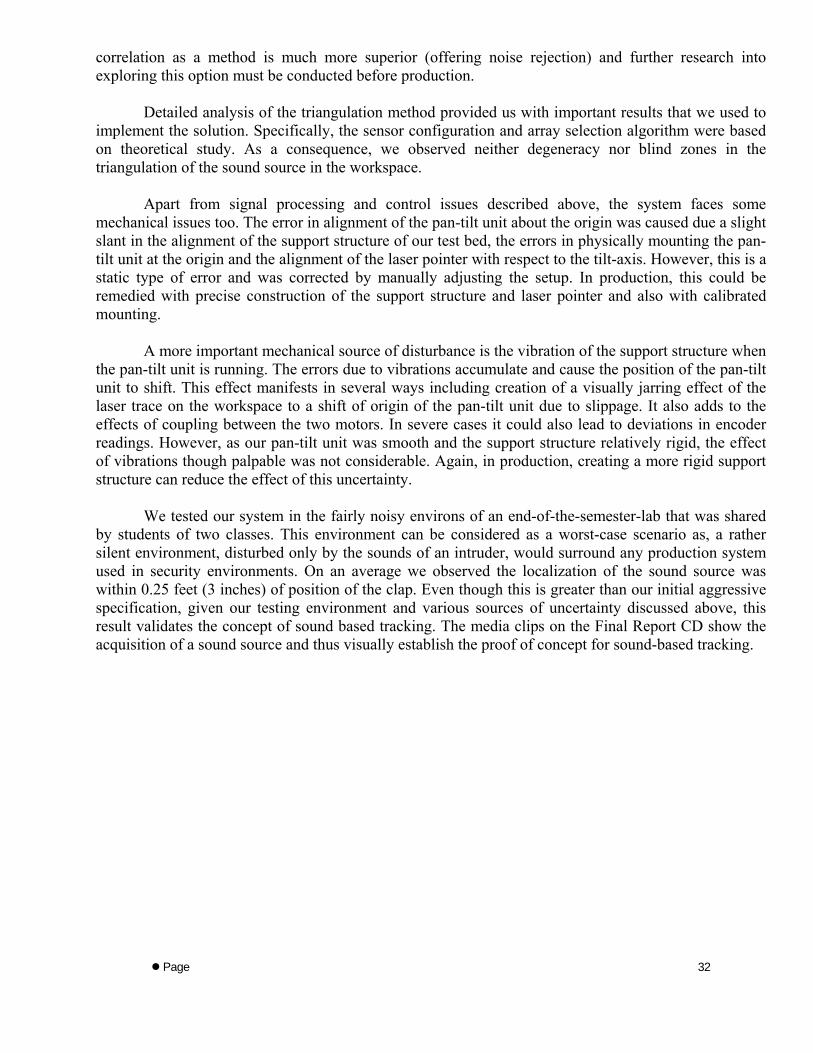
7 Conclusions The system was an overall success as we achieved many of our goals from the project proposal. We proved that the theory behind sound based tracking using TDOA methods is a valid concept and can be implemented. Table 6 shows the specifications from all parts of the project. It also indicates the status of individual specifications. Pan Desired Specification Achieved Specification Result Maximum Overshoot

5% 1% MET

Rise Time < 0.3 s 0.15 s MET Settling Time < 0.4 s 0.2 s MET Steady State Error 0 0 (approx) MET Tracking < 10% at 3 Hz < 10% at 2 Hz

< 15% at 3 Hz ACCEPTABLE

Tilt Desired Specification Achieved Specification Result Maximum Overshoot

5% 0% MET

Rise Time < 0.4 s 0.5 s ACCEPTABLE Settling Time < 0.5 s 0.6 s ACCEPTABLE Steady State Error 0 0 (approx) MET Tracking < 10% at 3 Hz < 10% at 3 Hz MET Other Desired Specification Achieved Specification Result Sound Capture Freq

< 5000Hz < 5000 Hz MET

Sampling Freq 10 kHz 10kHz MET System Operation Real Time Not Real Time NOT MET Motion 3 Types 1 Type NOT MET

Table 7 – Achieved Specifications

The controller designed for the pan worked very well. It moved quickly to its target with little overshoot and no steady state error and we were very pleased with that. The controller designed for the tilt axis was a bit sluggish. If we had more time we believe we could have designed a more aggressive controller for the tilt that would have met our specifications, but regardless, the achieved specifications came very close to those desired for the tilt controller.

In regards to tracking, we were able to track 3 Hz with less than 10% error for the tilt controller but for the pan controller we could only get less than 10% error for 2 Hz. We believe because our controller for pan was so aggressive, it could not maintain a 3 Hz tracking frequency with less than 10% error in the amplitude.

There were also many other specifications set throughout the project. We desired to capture a sound anywhere from 20-5000 Hz and then sample that sound at 10 kHz both of which were accomplished nicely. We had desired to run our system in real-time to better show how this could enhance practical security measures, but we could not have the target computer running the xPC Target system while simultaneously solving our TDOA and triangulation equations. For our purpose, we chose to sample the microphones for one second, and then stop the system to do calculations, and finally start the system again to point at the desired co-ordinates. We had hoped using the real time application of this project to investigate continuous and

Page

35

random motions with our tracking machine; however, because we did not implement the real time operation, we could not investigate these motions. In practical security settings the real time implementation of this machine is obviously needed for any hope detecting a security breach or intruder. Overall, our project demonstrates that this is a viable technique for use in security applications.

Page

36

8 Bibliography

[1] P. Aarabi, "The Fusion of Distributed Microphone Arrays for Sound Localization," EURASIP Journal of Applied Signal Processing, Vol. 2003, No. 4, pp. 338-347, March 2003.

[2] Muhammad Aatique, Evaluation Of TDOA Techniques For Position Location In CDMA Systems, Master of Science Thesis, Virginia Polytechnic Institute and State University, September 1997.

[3] Robert J. Schilling, Fundamentals of Robotics: Analysis and Control, New Jersey: Prentice-Hall, 1990, pp. 202-203.

[4] Kevin Murphy et al., SOUND TRACKING PAN-TILT MACHINE, Project Proposal for ECSE 4962 Control Systems Design, Rensselaer Polytechnic Institute, February 2004.

[5] Kevin Murphy et al., SOUND TRACKING PAN-TILT MACHINE, Progress Report for ECSE 4962 Control Systems Design, Rensselaer Polytechnic Institute, February 2004.

[6] K.J Astrom et al., “Friction Models and Friction Compensation”. http://www.cat.rpi.edu/~wen/ECSE4962S04/astrom_friction.pdf

[7] G.Liu, “On Velocity Estimation Using Position Measurements”, Proceedings of the American Control Conference, Anchorage, AK May 8-10, 2002

[8] Y. Zhang et al., “Friction Compensation with Estimated Velocity”, proceedings of the 2002 IEEE International Conference on robotics & automation Washington DC May 2002

Page

37

Appendix A - Team Member Contribution

Task/Chapter Primary Contributor Executive Summary Kevin Murphy Introduction Kevin Murphy Professional and Societal Consideration Kevin Murphy Design Procedure

Modeling Matthew Daigle Control System Matthew Daigle Sensor System Matthew Daigle System Integration Matthew Gates Design Details Modeling Matthew Daigle Control Matthew Daigle Microphones Matthew Gates Time Difference of Arrival Matthew Gates Triangulation Vadiraj Hombal System Integration Vadiraj Hombal Design Verification

Model Verification Matthew Daigle Control Validation Vadiraj Hombal TDOA and Triangulation Vadiraj Hombal

Costs and Schedule Kevin Murphy Conclusion Kevin Murphy Report Integration Kevin Murphy

All members of the team contributed to editing and revisions to each section. Matthew Gates was responsible for inertia identification, microphone testing and setup, and test bed construction. Matthew Daigle, Kevin Murphy, Vadiraj Hombal were responsible for modeling and control. Vadiraj Hombal was also responsible for triangulation algorithm and uncertainty analysis. While these members took the lead on certain design aspects, all team members gave input on all parts.

____________________________ Kevin Murphy ____________________________

Matthew Gates ____________________________ Vadiraj Hombal ____________________________

Matthew Daigle

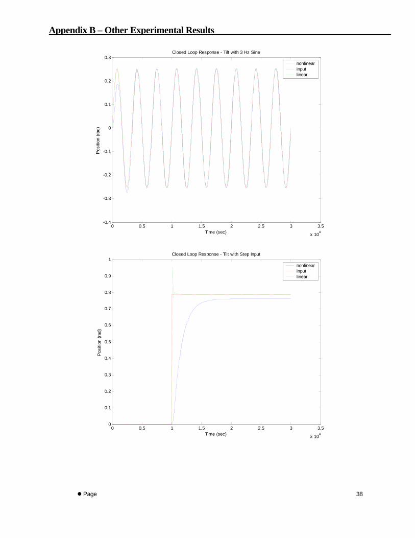
Appendix B – Other Experimental Results

0 0.5 1 1.5 2 2.5 3 3.5

x 104

-0.4

-0.3

-0.2

-0.1

0

0.1

0.2

0.3

Pos

ition

(rad

)

Time (sec)

Closed Loop Response - Tilt with 3 Hz Sine

nonlinearinputlinear

0 0.5 1 1.5 2 2.5 3 3.5

x 104

0

0.1

0.2

0.3

0.4

0.5

0.6

0.7

0.8

0.9

1Closed Loop Response - Tilt with Step Input

Pos

ition

(rad

)

Time (sec)

nonlinearinputlinear

Page

38

0 1 2 3 4 5 6

x 104

-1

-0.8

-0.6

-0.4

-0.2

0

0.2

0.4

0.6

0.8

1

Pos

ition

(rad

)

Closed Loop Response - Pan with 2 Hz Sine one Actual System

Time (0.0001 sec samples)

actual desired

0 0.5 1 1.5 2 2.5 3 3.5-0.5

0

0.5

1

1.5

2

2.5

3

3.5

Pos

ition

(rad

)

Closed Loop Response - Pan Axis with Step Input

Time (sec)

actual desired

Page

39

0 1 2 3 4 5 6

x 104

-1.5

-1

-0.5

0

0.5

1

1.5

Pos

ition

(rad

)

Closed Loop Response - Tilt to 3 Hz Sine

Time (0.0001 sec samples)

actual desired

0 0.5 1 1.5 2 2.5 3 3.50

0.1

0.2

0.3

0.4

0.5

0.6

0.7

0.8

Pos

ition

(rad

)

Closed Loop Response - Tilt with Step Input on Actual System

Time (sec)

actual desired

Page

40

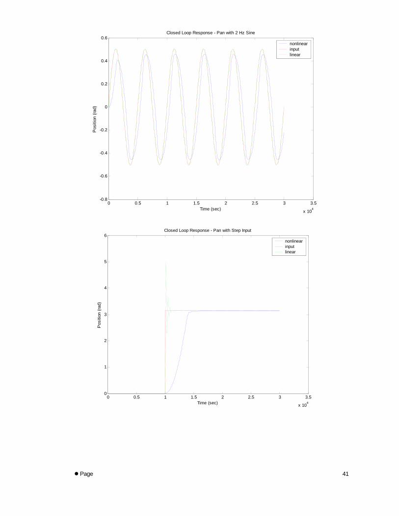
0 0.5 1 1.5 2 2.5 3 3.5

x 104

-0.8

-0.6

-0.4

-0.2

0

0.2

0.4

0.6

Time (sec)

Pos

ition

(rad

)

Closed Loop Response - Pan with 2 Hz Sine

nonlinearinputlinear

0 0.5 1 1.5 2 2.5 3 3.5

x 104

0

1

2

3

4

5

6

Time (sec)

Pos

ition

(rad

)

Closed Loop Response - Pan with Step Input

nonlinearinputlinear

Page

41

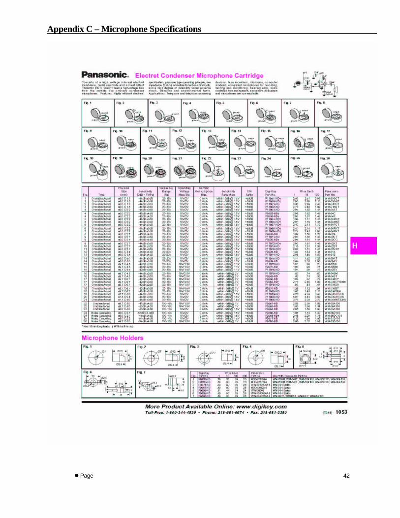
Appendix C – Microphone Specifications

Page

42

Page

43

Page

44

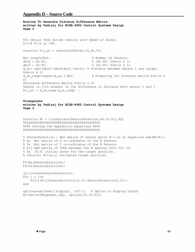
Appendix D – Source Code Routine To Generate Distance Difference Matrix. written by Vadiraj for ECSE-4962 Control Systems Design Team 3 %To obtain TDOA divide results with Speed of Sound. %1134 Ft/S at 74F. function Dij_st = simulateTDOA(Xs,Ys,Xt,Yt) Ns= length(Xs); % Number of Sensors. delX = Xs-Xt; % (Xi-Xt) Dim=(n x 1) delY = Ys-Yt; % (Yi-Yt) Dim=(n x 1) d_st= sqrt(delX.*delX+delY.*delY); % Distance between Sensor i and target. Dim=(n x 1) d_st_temp=repmat(d_st,1,Ns); % Preparing for distance matrix Dim=(n x n) %Distance difference Matrix Dim=(n x n) %where (i,j)th element is the difference in distance betn sensor i and j Dij_st = d_st_temp-d_st_temp' ; Triangulate written by Vadiraj for ECSE-4962 Control Systems Design Team 3

function Xt = triangulate(SensorSelection,Xs,Ys,Dij,Xg) %%%%%%%%%%%%%%%%%%%%%%%%%%%%%%%%%%%%%%%%%% %%%% Solving the Hyperbolic Equations %%%% %%%%%%%%%%%%%%%%%%%%%%%%%%%%%%%%%%%%%%%%%% % SensorSelection : Mx2 matrix of sensor pairs M = no of equations max(M)=N-1. % Xs Nx1 matrix of X co-ordinates of the N Sensors % Ys Nx1 matrix of Y co-ordinates of the N Sensors % Dij NxN matrix of TDOA between the N sensors with Dii =0; % Xg [X,Y] initial guess for the target position. % returns: Xt=[x,y] estimated target position. P1=Xs(SensorSelection); P2=Ys(SensorSelection); [m,n]=size(SensorSelection); for i = 1:m P3(i)=Dij(SensorSelection(i,1),SensorSelection(i,2)); end options=optimset('Display','off'); % Option to display output Xt=fsolve(@hypeqns,[Xg], options,P1,P2,P3);

Page

45

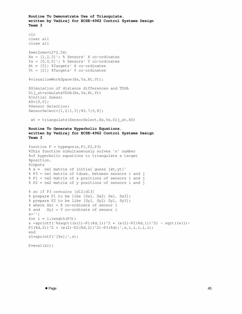
Routine To Demonstrate Use of Triangulate. written by Vadiraj for ECSE-4962 Control Systems Design Team 3 clc clear all close all feet2cms=12*2.54; Xs = [1,2,3]'; % Sensors' X co-ordinates Ys = [0,0,0]'; % Sensors' Y co-ordinates Xt = [5]; %Targets' X co-ordinates Yt = [2]; %Targets' Y co-ordinates %visualizeWorkSpace(Xs,Ys,Xt,Yt); %Simulation of distance differences and TDOA Dij_st=simulateTDOA(Xs,Ys,Xt,Yt) %Initial Guess: X0=[0,0]; %Sensor Selection: SensorSelect=[1,2;1,3];%5,7;5,8]; xt = triangulate(SensorSelect,Xs,Ys,Dij_st,X0) Routine To Generate Hyperbolic Equations. written by Vadiraj for ECSE-4962 Control Systems Design Team 3 function F = hypeqns(x,P1,P2,P3) %This function simultaneously solves 'n' number %of hyperbolic equations to triangulate a target %position. %inputs % x = nx1 matrix of initial guess [xt,yt]' % P3 = nx1 matrix of tdoas. between sensors i and j % P1 = nx2 matrix of x positions of sensors i and j % P2 = nx2 matrix of y positions of sensors i and j % so if P3 contains [d12;d13] % prepare P1 to be like [Sx1, Sx2; Sx1, Sx3]; % prepare P2 to be like [Sy1, Sy2; Sy1, Sy3]; % where Sxi = X co-ordinate of sensor i % and Syi = Y co-ordinate of sensor i s=''; for i = 1:length(P3); s =sprintf('%ssqrt((x(1)-P1(%d,1))^2 + (x(2)-P2(%d,1))^2) - sqrt((x(1)-P1(%d,2))^2 + (x(2)-P2(%d,2))^2)-P3(%d);',s,i,i,i,i,i); end s1=sprintf('[%s];',s); F=eval(s1);

Page

46

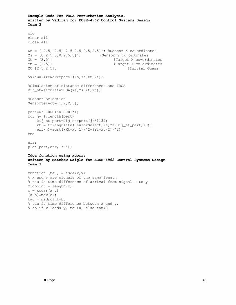
Example Code For TDOA Perturbation Analysis. written by Vadiraj for ECSE-4962 Control Systems Design Team 3 clc clear all close all Xs = [-2.5,-2.5,-2.5,2.5,2.5,2.5]'; %Sensor X co-ordinates Ys = [0,2.5,5,0,2.5,5]'; %Sensor Y co-ordinates Xt = [2.5]; %Target X co-ordinates Yt = [1.5]; %Target Y co-ordinates X0=[2.5,2.5]; %Initial Guess %visualizeWorkSpace1(Xs,Ys,Xt,Yt); %Simulation of distance differences and TDOA Dij_st=simulateTDOA(Xs,Ys,Xt,Yt); %Sensor Selection SensorSelect=[1,2;2,3]; pert=0:0.0001:0.0001*1; for j= 1:length(pert) Dij_st_pert=Dij_st+pert(j)*1134; xt = triangulate(SensorSelect,Xs,Ys,Dij_st_pert,X0); err(j)=sqrt((Xt-xt(1))^2+(Yt-xt(2))^2); end err; plot(pert,err,'*-'); Tdoa function using xcorr: written by Matthew Daigle for ECSE-4962 Control Systems Design Team 3 function [tau] = tdoa(x,y) % x and y are signals of the same length % tau is time difference of arrival from signal x to y midpoint = length(x); c = xcorr(x,y); [a,b]=max(c); tau = midpoint-b; % tau is time difference between x and y, % so if x leads y, tau>0, else tau<0

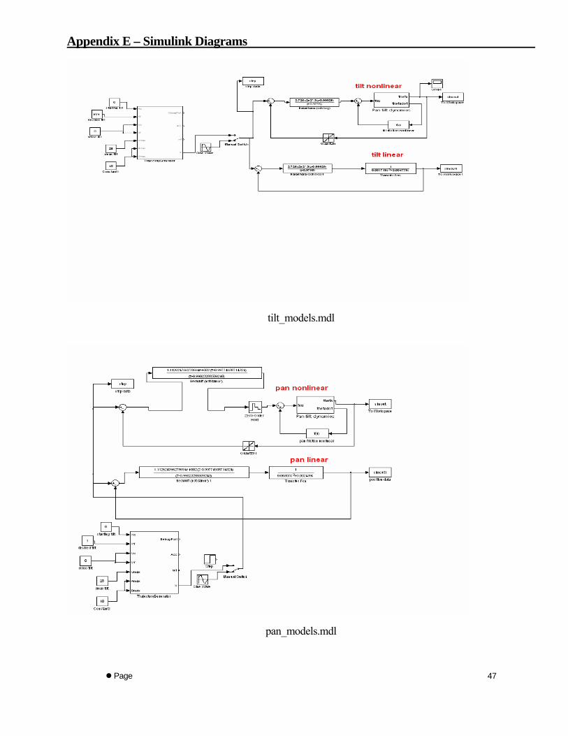
Appendix E – Simulink Diagrams

tilt_models.mdl

pan_models.mdl

Page

47

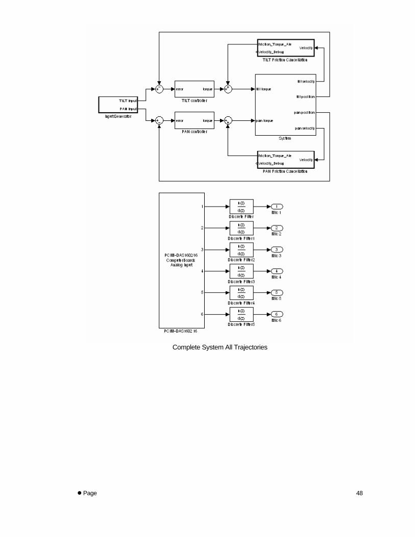
Complete System All Trajectories

Page

48

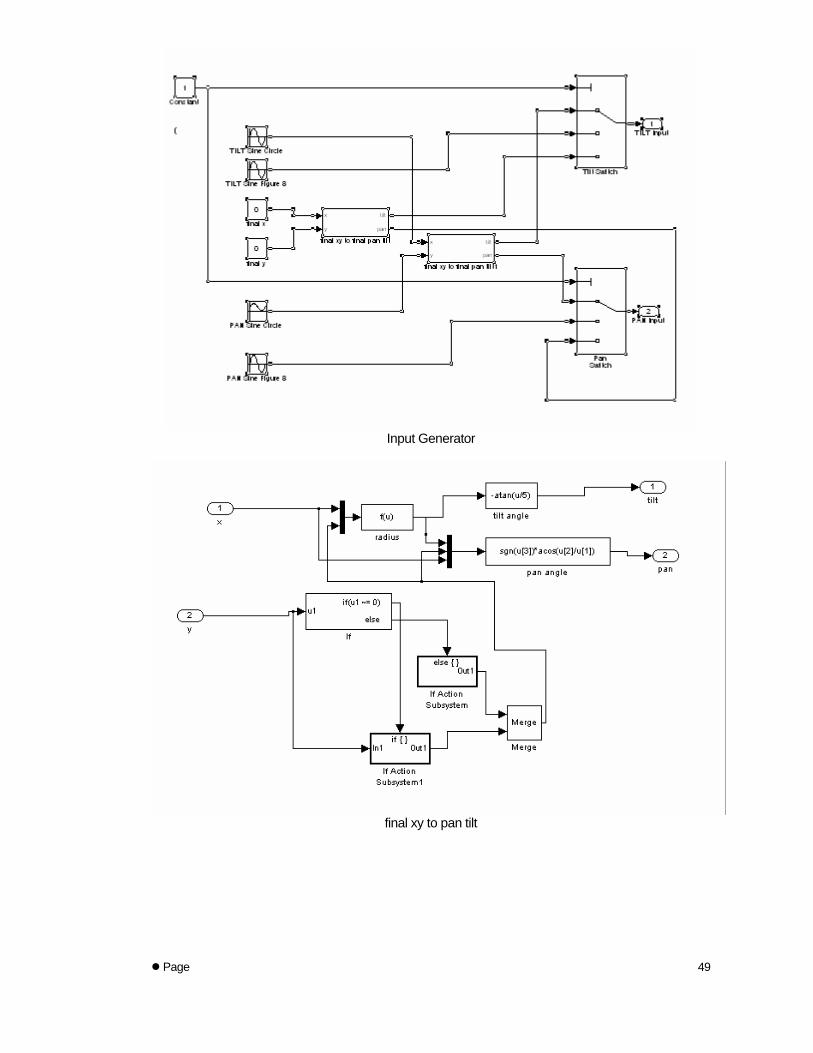
Input Generator

final xy to pan tilt

Page

49

if action subsystem

if action subsystem1

final xy to pan tilt1

Page

50

pan controller

pan friction cancellation

System

Page

51

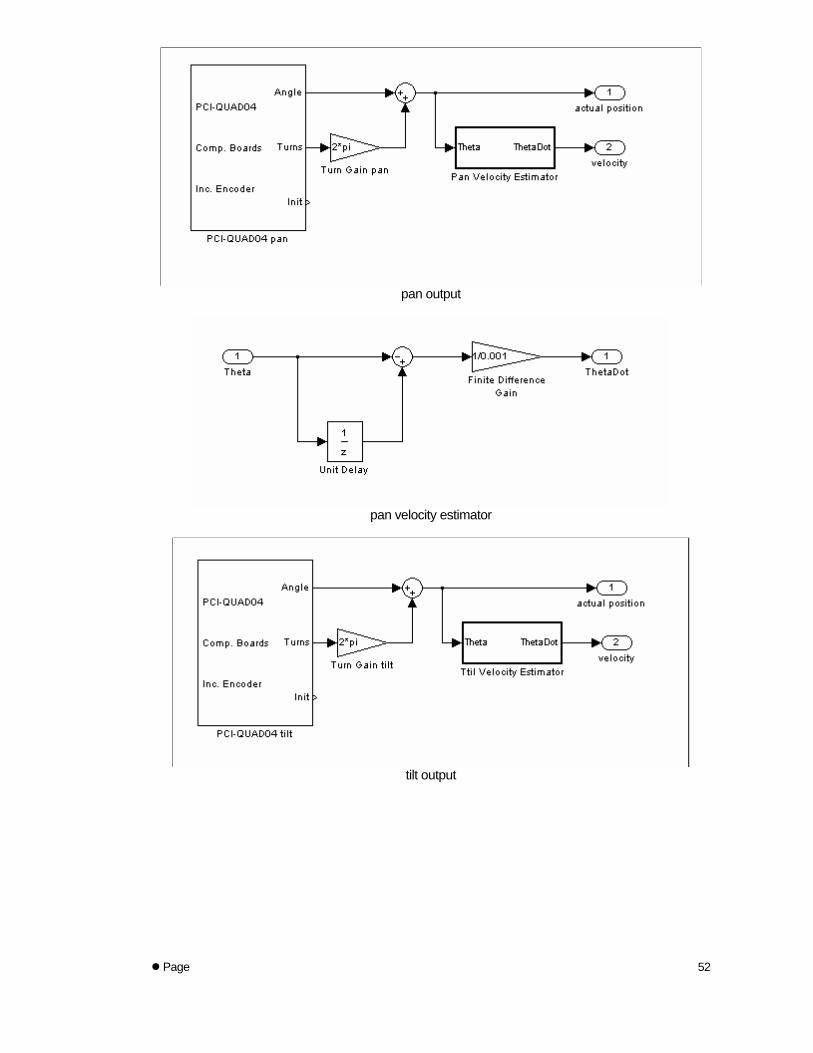
pan output

pan velocity estimator

tilt output

Page

52

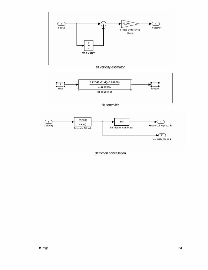
tilt velocity estimator

tilt controller

tilt friction cancellation

Page

53

Page

54

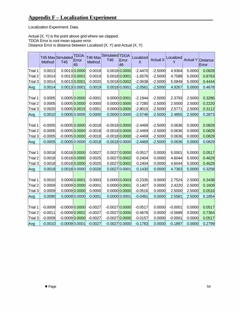
Appendix F – Localization Experiment

Localization Experiment: Data. Actual (X, Y) is the point above grid where we clapped. TDOA Error is root mean square error. Distance Error is distance between Localized (X, Y) and Actual (X, Y)

Simulated T46

T45 Max Method

Simulated T45

TDOA Error 45

T46 Max Method

TDOA Error 46

Localized X Actual X Localized

Y Actual Y Distance Error

Trial 1 0.0013 0.0013 0.0000 0.0018 0.0018 0.0000 -2.4470 -2.5000 4.9364 5.0000 0.0828Trial 2 0.0014 0.0013 0.0001 0.0019 0.0018 0.0001 -1.6576 -2.5000 4.7588 5.0000 0.8763Trial 3 0.0014 0.0013 0.0001 0.0020 0.0018 0.0002 -2.0638 -2.5000 5.0849 5.0000 0.4444Avg 0.0014 0.0013 0.0001 0.0019 0.0018 0.0001 -2.0561 -2.5000 4.9267 5.0000 0.4678 Trial 1 0.0005 0.0005 0.0000 -0.0001 0.0000 0.0001 -2.1944 -2.5000 2.3793 2.5000 0.3286Trial 2 0.0005 0.0005 0.0000 0.0000 0.0000 0.0000 -2.7280 -2.5000 2.5000 2.5000 0.2220Trial 3 0.0020 0.0005 0.0015 0.0001 0.0000 0.0000 -2.8015 -2.5000 2.5771 2.5000 0.3112Avg 0.0010 0.0005 0.0005 0.0000 0.0000 0.0000 -2.5746 -2.5000 2.4855 2.5000 0.2873 Trial 1 -0.0005 -0.0005 0.0000 -0.0018 -0.0018 0.0000 -2.4469 -2.5000 0.0636 0.0000 0.0829Trial 2 -0.0005 -0.0005 0.0000 -0.0018 -0.0018 0.0000 -2.4469 -2.5000 0.0636 0.0000 0.0829Trial 3 -0.0005 -0.0005 0.0000 -0.0018 -0.0018 0.0000 -2.4469 -2.5000 0.0636 0.0000 0.0829Avg -0.0005 -0.0005 0.0000 -0.0018 -0.0018 0.0000 -2.4469 -2.5000 0.0636 0.0000 0.0829 Trial 1 0.0018 0.0018 0.0000 0.0027 0.0027 0.0000 -0.0517 0.0000 5.0001 5.0000 0.0517Trial 2 0.0018 0.0018 0.0000 0.0025 0.0027 0.0002 0.2404 0.0000 4.6044 5.0000 0.4629Trial 3 0.0018 0.0018 0.0000 0.0025 0.0027 0.0002 0.2404 0.0000 4.6044 5.0000 0.4629Avg 0.0018 0.0018 0.0000 0.0026 0.0027 0.0001 0.1430 0.0000 4.7363 5.0000 0.3258 Trial 1 0.0010 0.0009 0.0001 0.0003 0.0000 0.0003 -0.2335 0.0000 2.7524 2.5000 0.3438Trial 2 0.0009 0.0009 0.0000 -0.0001 0.0000 0.0001 0.1407 0.0000 2.4220 2.5000 0.1609Trial 3 0.0009 0.0009 0.0000 0.0000 0.0000 0.0000 -0.0516 0.0000 2.5000 2.5000 0.0516Avg 0.0090 0.0009 0.0000 0.0001 0.0000 0.0001 -0.0481 0.0000 2.5581 2.5000 0.1854 Trial 1 -0.0009 -0.0009 0.0000 -0.0027 -0.0027 0.0000 -0.0517 0.0000 -0.0001 0.0000 0.0517Trial 2 -0.0011 -0.0009 0.0002 -0.0027 -0.0027 0.0000 -0.4676 0.0000 -0.5689 0.0000 0.7364Trial 3 -0.0009 -0.0009 0.0000 -0.0027 -0.0027 0.0000 -0.0157 0.0000 -0.0001 0.0000 0.0517Avg -0.0010 -0.0009 0.0001 -0.0027 -0.0027 0.0000 -0.1783 0.0000 -0.1897 0.0000 0.2799

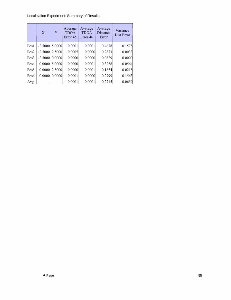
Localization Experiment: Summary of Results

X Y Average TDOA

Error 45

Average TDOA

Error 46

Average Distance

Error

Variance Dist Error

Pos1 -2.5000 5.0000 0.0001 0.0001 0.4678 0.1578Pos2 -2.5000 2.5000 0.0005 0.0000 0.2873 0.0033Pos3 -2.5000 0.0000 0.0000 0.0000 0.0829 0.0000Pos4 0.0000 5.0000 0.0000 0.0001 0.3258 0.0564Pos5 0.0000 2.5000 0.0000 0.0001 0.1854 0.0218Pos6 0.0000 0.0000 0.0001 0.0000 0.2799 0.1563Avg 0.0001 0.0001 0.2715 0.0659

Page

55

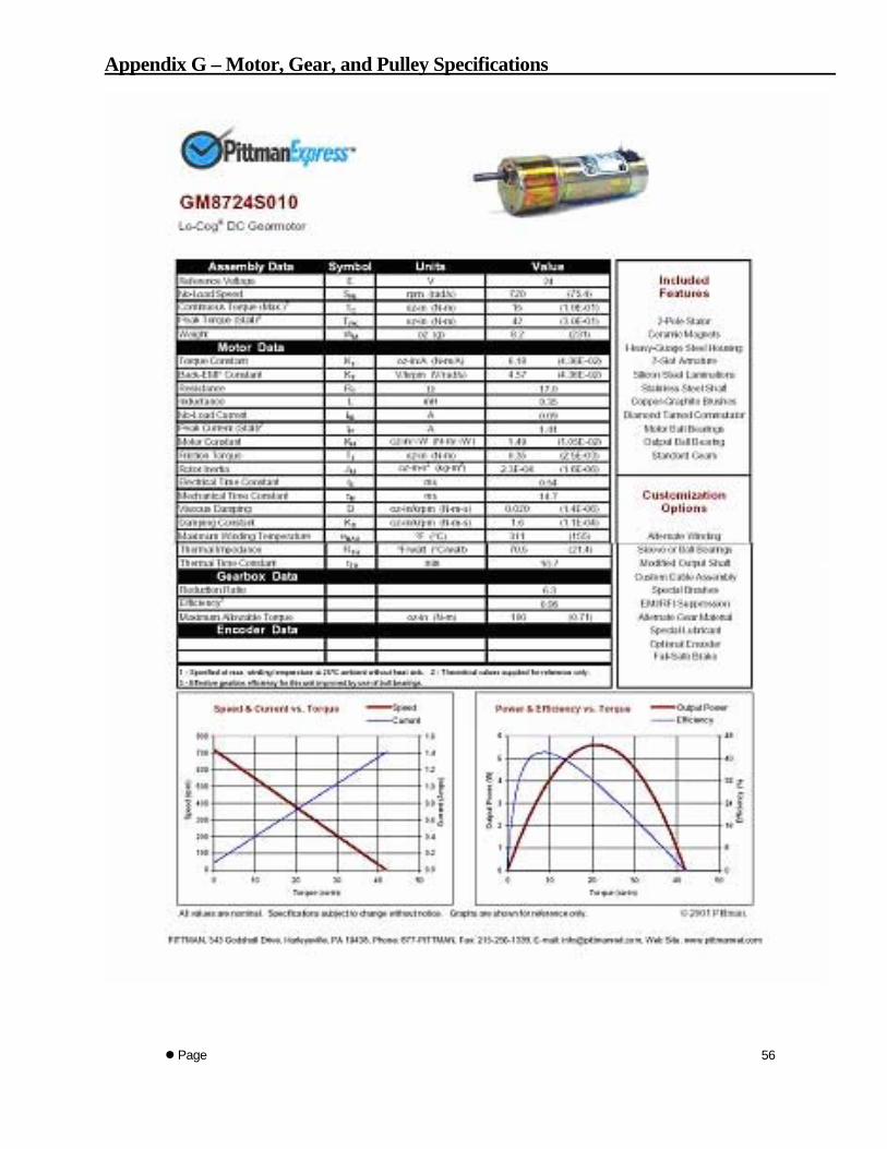
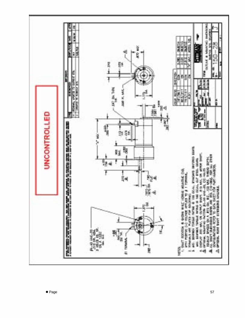
Appendix G – Motor, Gear, and Pulley Specifications

Page

56

Page

57