Sound source localization – state of the art and new

Elektrotechnik & Informationstechnik (2021) 138/3: 229–243. https://doi.org/10.1007/s00502-021-00881-6 ORIGINALARBEIT

Sound source localization – state of the artand new inverse schemeS. Gombots, J. Nowak , M. Kaltenbacher

Acoustic source localization techniques in combination with microphone array measurements have become an important tool for noisereduction tasks. A common technique for this purpose is acoustic beamforming, which can be used to determine the source locationsand source distribution. Advantages are that common algorithms such as conventional beamforming, functional beamforming ordeconvolution techniques (e.g., Clean-SC) are robust and fast. In most cases, however, a simple source model is applied and theGreen’s function for free radiation is used as transfer function between source and microphone. Additionally, without any furthersignal processing, only stationary sound sources are covered. To overcome the limitation of stationary sound sources, two approachesof beamforming for rotating sound sources are presented, e.g., in an axial fan.

Regarding the restrictions concerning source model and boundary conditions, an inverse method is proposed in which the waveequation in the frequency domain (Helmholtz equation) is solved with the corresponding boundary conditions using the finite elementmethod. The inverse scheme is based on minimizing a Tikhonov functional matching measured microphone signals with simulatedones. This method identifies the amplitude and phase information of the acoustic sources so that the prevailing sound field can bewith a high degree of accuracy.

Keywords: sound source localization; inverse scheme; rotating beamforming; beamforming

Schallquellenlokalisation: state of the art und neues inverses Verfahren.

Die Lokalisation von akustischen Schallquellen mithilfe von Schalldruckmessungen unter Verwendung von Mikrofonarrays ist ein wich-tiges Instrument in der Lärmbekämpfung. Ein weit verbreitetes Verfahren ist hierbei das akustische Beamforming, mit dem sowohldie Quellpositionen als auch -verteilungen bestimmt werden können. Bekannte Algorithmen, wie Standard-Beamforming, Functional-Beamforming oder Entfaltungsmethoden (wie z. B. Clean-SC) haben den Vorteil, dass sie robust und schnell in der Berechnung sind.Nachteilig ist hingegen, dass meist ein simples Modell für die akustischen Quellen angenommen wird, und dass die Green’scheFunktion für freie Schallabstrahlung als Transferfunktion zwischen Quell- und Mikrofonpositionen verwendet wird. Außerdem kön-nen bewegte Schallquellen nicht ohne weitere Signalverarbeitungsschritte lokalisiert werden. In diesem Zusammenhang werden zweiMethoden für rotierende Schallquellen, wie sie z. B. bei einem rotierenden Ventilator vorkommen, präsentiert.

Für eine akkurate Berücksichtigung der Messumgebung und um die Einschränkungen bezüglich des vereinfachten Quellenmodellsund der Randbedingungen der Messumgebung zu überwinden, wird ein inverses Verfahren präsentiert, in dem die Wellengleichungim Frequenzbereich (Helmholtz-Gleichung) mit entsprechenden Randbedingungen mittels der Finite Elemente-Methode gelöst wird.Dieses Verfahren basiert auf einem Tikhonov-Funktionals, das die Differenz zwischen Mikrofonmessungen und den simulierten Schall-drücken minimiert. Mit dieser inversen Methode können die Schallquellen in Amplitude und Phase identifiziert werden, sodass dasvorherrschende Schallfeld mit hoher Genauigkeit rekonstruiert werden kann.

Schlüsselwörter: Schallquellenlokalisation; inverses Verfahren; Beamforming; rotierendes Beamforming

Received February 9, 2021, accepted March 12, 2021, published online March 25, 2021© The Author(s) 2021

1. IntroductionTypically, sound emissions from technical applications and produc-tion machines are perceived as disturbing noise. When trying tosolve noise problems or refine the acoustic design of a prod-uct, knowledge of the position and distribution of sound sourcesis necessary. In this context, one of the biggest challenges innoise and vibration problems is to identify the areas of a de-vice, machine or structure that produce the significant acousticemission. For this task various sound localization methods can beused, in order to localize and visualize sound sources. The in-formation will be given in so-called source maps, which provideinformation about location, distribution and strength of soundsources.

The standard methods are intensity measurements, acoustic near-field holography and acoustic beamforming. But, these methodsare not universally applicable. In contrast to intensity measure-

ments, where an intensity probe is used, near-field holography and

beamforming use locally distributed microphones (= microphone

array). Depending on the measurement object, frequency range

and measurement environment, the different methods have specific

strengths and weaknesses.

In the last years, considerable improvements have been achieved

in the localization of sound sources using microphone arrays. How-

ever, there are still some limitations. In most cases, a simple source

model is applied and the Green’s function for free radiation is used

as transfer function between source and microphone. Hence, the

Juni 2021 138. Jahrgang © The Author(s) heft 3.2021

Gombots, Stefan, TU Wien, Institute of Mechanics and Mechatronics, Wien, Austria(E-mail: [email protected]); Nowak, Jonathan, TU Wien, Institute ofMechanics and Mechatronics, Wien, Austria; Kaltenbacher, Manfred, TU Graz, Instituteof Fundamentals and Theory in Electrical Engineering, Graz, Austria

229

http://orcid.org/0000-0001-8403-693X

http://crossmark.crossref.org/dialog/?doi=10.1007/s00502-021-00881-6&domain=pdf

mailto:[email protected]

ORIGINALARBEIT S. Gombots et al. Sound source localization – state of the art and new inverse scheme

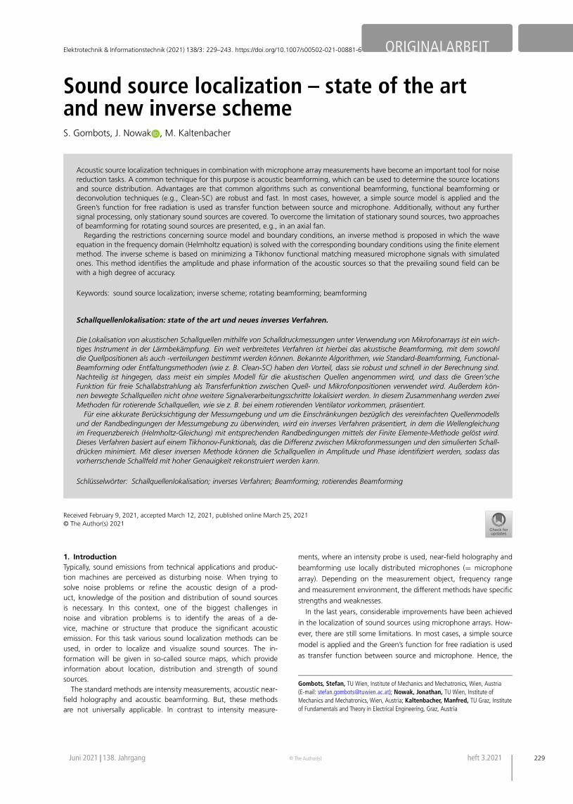
Fig. 1. Parameters: Distance to scanning area Z = 1 m, array aperture W = 1 m, source frequency f = 4000 Hz, microphone spacing �M = 0.1 mand discretization of the focus grid � = 1 mm

actual conditions as given in the measurement setup are not takeninto account.

In real life applications, one may also be faced with moving soundsources, e.g. a passing vehicle or a rotating fan. Here, the men-tioned sound source localization algorithms and methods do notreadily apply, but there exist advanced signal processing methodsthat overcome the limitation to stationary sound sources.

2. Beamforming based algorithmThe acoustic field, described by the complex acoustic pressure p̃a

of a monopole source with source strength σ , is calculated in thefrequency domain with Green’s function g̃(r) of free radiation by

p̃a(x,y,ω) = σ (y) g̃(r) = σ (y)e−j ω

c0r

4πrwith r = |x − y|, (1)

where x denotes the observer position (e.g. microphone positions)and y the source postions, c0 the speed of sound and ω = 2πf theangular sound frequency. All measured microphone signals pa(t) areFourier transformed and the resulting complex pressure values p̃a ata certain frequency ω are stored in a vector

p̃a(ω) =

⎡

⎢

⎢

⎣

p̃a,1(ω)...

p̃a,M(ω)

⎤

⎥

⎥

⎦

.

The cross-spectral matrix (CSM) is calculated by

˜C(ω) = p̃a(ω) p̃Ha (ω) , (2)

with �H the hermitian operation (transposition and complex conju-gation).

In Conventional Beamforming (ConvBF), the fundamental andmost basic as well as robust frequency domain processing method[1], the measured sound field is compared to a calculated soundfield. Thereby, a certain model for the acoustic source is as-sumed. Most beamforming algorithms model the acoustic sourceby monopols (1) to calculate the acoustic pressure. By using thisacoustic source model, following functional is defined

J (σ 2) = ||˜C − σ 2g̃ g̃H||2F , (3)

which refers to a single source with the strength σ to be determined(without loss of generality). Here, g̃ denotes the vector of the indi-vidual Green’s functions (also called steering vector) and ||�||F is theFrobenius norm. Minimizing the functional (3), i.e. setting its deriva-tive to zero, yields

σ (y) =√

√

√

√

√

g̃H˜Cg̃

(

g̃Hg̃)2

=√

w̃H˜Cw̃ with w̃ = g̃

g̃Hg̃, (4)

which is the expression for the determination of the source strength.Thereby, w̃ denotes the weighted steering vector. The steering vec-tor represents the transfer functions from the focus point to the mi-crophone positions and account for the phase shift and amplitudecorrection (sound propagation model) as well as the microphoneweighting [2]. They can be either obtained by measurements [3] orby theoretical models. In [4], different steering vector formulationsare discussed. Thereby, a reasonable enhancement in the correct es-timation of the source location could be obtained, whereas there isa trade-off between the correct reconstruction of the location andthe source strength. Another approach of determining the transferfunction is given by combining measurement and simulation, lead-ing to numerically calculated transfer functions (NCTFs) [5, 6].

The main diagonal elements of the CSM (2) represent the autopower of the microphones and therefore provide no informationabout the phase differences between the microphones, but may in-troduce microphone self noise. Hence, for experimental measure-ments, the main diagonal is usually omitted.

For broadband sound sources it may be of interest to plot sourcemaps in frequency bands (e.g., one-third or octave bands), ratherthan for single frequencies. For this purpose the individual sourcemaps are energy summed [7] for each frequency band according to

σn =√

√

√

√

Nf∑

i=1

σ 2n,i , (5)

whereby Nf denotes the number of frequencies in the consideredband.

In Fig. 1a the source map (calculated by (4)) of the geometricsetup given in Fig. 1b is depicted. Here, for the localization a line

230 heft 3.2021 © The Author(s) e&i elektrotechnik und informationstechnik

S. Gombots et al. Sound source localization – state of the art and new inverse scheme ORIGINALARBEIT

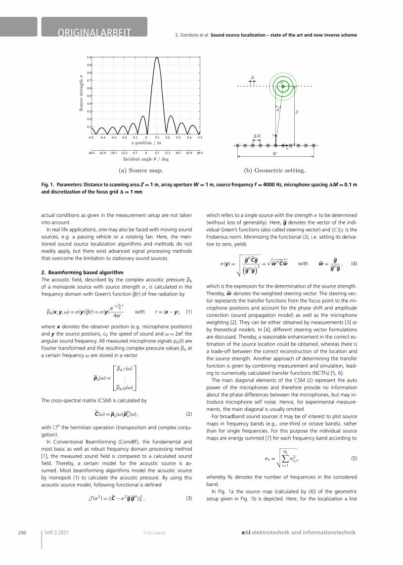
Fig. 2. Schematic representation of a Point Spread Function (PSF) in (a) for a line array (1D) and in (b) for a ring array (2D)

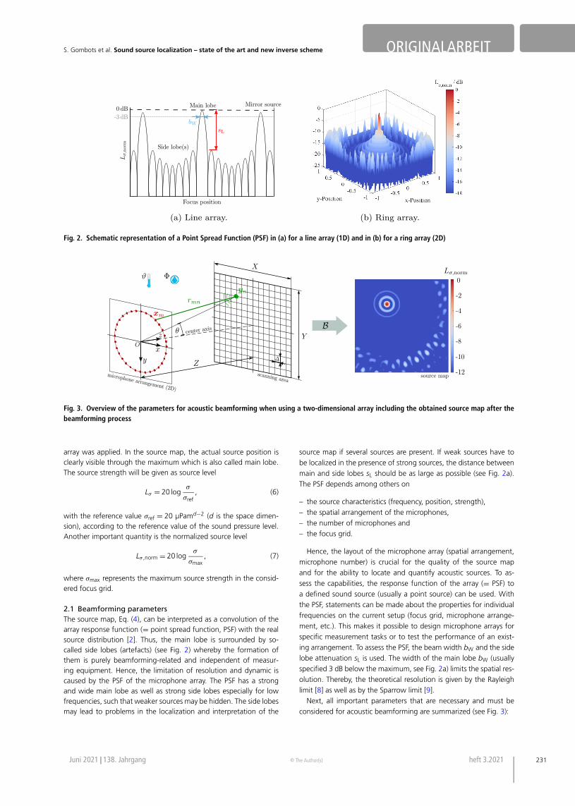
Fig. 3. Overview of the parameters for acoustic beamforming when using a two-dimensional array including the obtained source map after thebeamforming process

array was applied. In the source map, the actual source position isclearly visible through the maximum which is also called main lobe.The source strength will be given as source level

Lσ = 20 logσ

σref, (6)

with the reference value σref = 20 µPamd−2 (d is the space dimen-sion), according to the reference value of the sound pressure level.Another important quantity is the normalized source level

Lσ ,norm = 20 logσ

σmax, (7)

where σmax represents the maximum source strength in the consid-ered focus grid.

2.1 Beamforming parametersThe source map, Eq. (4), can be interpreted as a convolution of thearray response function (= point spread function, PSF) with the realsource distribution [2]. Thus, the main lobe is surrounded by so-called side lobes (artefacts) (see Fig. 2) whereby the formation ofthem is purely beamforming-related and independent of measur-ing equipment. Hence, the limitation of resolution and dynamic iscaused by the PSF of the microphone array. The PSF has a strongand wide main lobe as well as strong side lobes especially for lowfrequencies, such that weaker sources may be hidden. The side lobesmay lead to problems in the localization and interpretation of the

source map if several sources are present. If weak sources have tobe localized in the presence of strong sources, the distance betweenmain and side lobes sL should be as large as possible (see Fig. 2a).The PSF depends among others on

– the source characteristics (frequency, position, strength),– the spatial arrangement of the microphones,– the number of microphones and– the focus grid.

Hence, the layout of the microphone array (spatial arrangement,microphone number) is crucial for the quality of the source mapand for the ability to locate and quantify acoustic sources. To as-sess the capabilities, the response function of the array (= PSF) toa defined sound source (usually a point source) can be used. Withthe PSF, statements can be made about the properties for individualfrequencies on the current setup (focus grid, microphone arrange-ment, etc.). This makes it possible to design microphone arrays forspecific measurement tasks or to test the performance of an exist-ing arrangement. To assess the PSF, the beam width bW and the sidelobe attenuation sL is used. The width of the main lobe bW (usuallyspecified 3 dB below the maximum, see Fig. 2a) limits the spatial res-olution. Thereby, the theoretical resolution is given by the Rayleighlimit [8] as well as by the Sparrow limit [9].

Next, all important parameters that are necessary and must beconsidered for acoustic beamforming are summarized (see Fig. 3):

Juni 2021 138. Jahrgang © The Author(s) heft 3.2021 231


– Array layout (microphone number M, microphone spacing �M,aperture W ),

– Focus (scan) grid (discretization �, dimension X and Y ),– Distance between microphone array and focus grid Z,– Temperature θ and relative air humidity � for the estimation of

c0,– Beamforming algorithm B,– Steering vector w̃ formulation.

2.2 Functional beamformingOne drawback of ConvBF is that the source map obtained with Con-vBF not only contains the main lobe, i.e. the peak in the source mapwhere the actual source is located, but also shows artefacts (sidelobes), which occur at positions without actual sources. This is dueto the above mentioned fact that the computed source distributionis a convolution of the real source distribution with the particularresponse function (PSF) of the array. While these side lobes have asmaller amplitude than the main lobe it is still possible that the sidelobes obscure weaker sources which are therefore not detected byConvBF. One possibility to reduce the high side lobe level is to usean advanced beamforming algorithm called Functional beamform-ing (FuncBF) [10, 11]. Here, a parameter ν is introduced and (4) ischanged to

σ =

√

√

√

√

√

√

√

(

g̃H˜C

1ν g̃

)ν

(

g̃Hg̃)ν+1

. (8)

The CSM is diagonalised according to

˜C = ˜U�˜UH

, (9)

with � = diag(

λ1ν

1 , . . . ,λ1ν

M

)

consisting of the eigenvalues λi of ˜C.

The case of ν = 1 leads to the equation for ConvBF. Using FuncBF,the dynamic range and the resolution of the source map can beimproved for increasing values of the parameter ν ≥ 1. In practice,using well calibrated arrays values of up to ν = 100 leads to satisfy-ing results [10].

2.3 Deconvolution algorithmsAnother way to overcome the drawback of side lobes in the sourcemap is to use advanced signal processing algorithms based on de-convolution, e.g., DAMAS [12], Clean-SC [13], SC-DAMAS [14] etc.,that convert the raw source map (4) into a deconvoluted sourcemap, resulting in higher resolution and dynamic range. Thereby, itis assumed that the computed source map obtained by (4) is builtup by individual scaled PSFs of the array. By using deconvolutionalgorithms, these response functions of the array are determinedand replaced by single peaks or narrow-width beams. As a conse-quence, the side lobes (artefacts) are removed in the deconvolvedmap. In [15] and [16], one can find a detailed comparison betweendifferent deconvolution techniques and the application to 2D and3D sound source localization. There, the different techniques arecompared with respect to position detection, source level estimationand computational time. The main findings for source localizationin a free radiation environment can be summarized as follows: (1)SC-DAMAS provides the best source map at highest computationalcosts; (2) Clean-SC has the best trade-off between fast computationand correct source detection. Usually, the deconvolution algorithmscan only be applied in post-processing because the calculation ofdeconvolved source maps takes too much time for real-time analy-ses.

2.4 Rotating beamformingIf the sound source is moving, i.e. the distance between soundsource and microphone (observer) is time dependent r = r(t) onehas to take into account that sound which is received at time t (=reception time) at an observation point x was emitted at an earliertime τ (= retarded time or emission time) from the source pointy. Further, a stationary observer perceives different sound frequen-cies than those that are emitted by the source, which is commonlyknown as the Doppler effect.

The retarded time is defined implicitly by

c0 (t − τ ) − r(τ ) = 0. (10)

For moving sound sources the presented methods for sound sourcelocalization can no longer be applied but there exist signal process-ing algorithms that treat special cases, e.g. translationally movingsound sources at constant speed U or sound sources rotating at anangular velocity Ω .

If we assume a time dependent monopole that moves along apath x = xs(t) the inhomogeneous wave equation in time domainreads as

1

c20

∂2pa

∂t2− �pa = q(x, t) = Q(t)δ(x − xs(t)). (11)

Its solution, i.e. the acoustic pressure of a moving monopole, can becalculated as [17]

pa(x, t) = Qe

4πre (1 − Me cosϑe)(12)

with

cosϑ = r · MrM

(13)

r(τ ) = x − xs(τ ); r = |r| (14)

M = 1c0

∂xs

∂t

∣

∣

∣

∣

τ

; M = |M|, (15)

where �e denotes evaluation at retarded time τ , M denotes thevectorial Mach number and ϑ the angle between the vector of thesource velocity c0M and the vector between source and observerr(τ ).

In the stationary case the sound pressure emitted by a monopolesource at location y is given as

pa(x, t) = Q(t − |x − y|/c0)4πr

. (16)

The factor 1/(1 − Me cosϑe) in the non-stationary case is alsocalled ’Doppler factor’ as the momentarily perceived sound fre-quency f (t) at the observer point of a sound source that emits soundat constant frequency f0 calculates as

f (t) = ddt

(f0τ ) = f0

1 − Me cosϑe. (17)

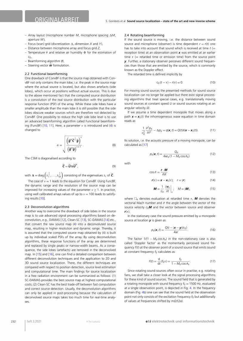
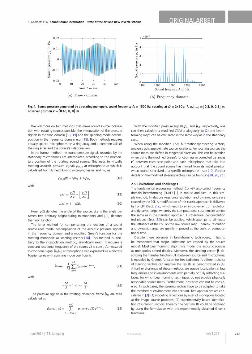
Since rotating sound sources often occur in practise, e.g. rotatingfans, we shall take a closer look at the signal processing algorithmsfor these kind of sound sources. The sound field that is generated bya rotating monopole with sound frequency f0 = 1500 Hz, evaluatedat a single observation point, is depicted in Fig. 4. In the frequencydomain (Fig. 4b) one can see that the sound field at the observationpoint not only consists of the excitation frequency f0 but additionallyof values at frequencies shifted by mΩ/(2π).



Fig. 4. Sound pressure generated by a rotating monopole, sound frequency f0 = 1500 Hz, rotating at Ω = 2π 30 s−1, xs|τ=0 = [0.3, 0, 0.5

]m,

observer position x = [0.45, 0, 0

]m

We will focus on two methods that make sound source localiza-tion with rotating sources possible, the interpolation of the pressuresignals in the time domain [18, 19] and the spinning mode decom-position in the frequency domain e.g. [18]. Both methods requiresequally spaced microphones on a ring array and a common axis ofthe ring array and the source’s rotational axis.

In the former method the sound pressure signals recorded by thestationary microphones are interpolated according to the momen-tary position of the rotating sound source. This leads to virtuallyrotating acoustic pressure signals pvr,m at microphone m which iscalculated from its neighboring microphones ml and mh as

pvr,m(t) = slpml + shpmh , (18)

with

sl(t) = ϕ(t)�ϕ

−⌊

ϕ(t)�ϕ

⌋

, (19)

sh(t) = 1 − sl(t). (20)

Here, ϕ(t) denotes the angle of the source, �ϕ is the angle be-tween two arbitrary neighbouring microphones and �� denotesthe floor function.

The latter method for compensating the rotation of a soundsource uses modal decomposition of the acoustic pressure signalsin the frequency domain and a modified Green’s function for therotating monopole as steering vectors [18]. This method is, con-trary to the interpolation method, analytically exact. It requires aconstant rotational frequency of the source Ω = const. A measuredmicrophone signal p̃m(ω) at microphone m is expressed via a discreteFourier series with spinning mode coefficients

p̃n(ω) = 1M

M∑

m=1

p̃m(ω) e−jnϕm , (21)

with

−M2

+ 1 ≤ n ≤ M2

. (22)

The pressure signals in the rotating reference frame p̃Ω are thencalculated as

p̃Ω (ϕm,ω) =M/2∑

n=−M/2+1

pn(ω + nΩ) e jnϕm . (23)

With the modified pressure signals p̃vr and p̃Ω , respectively, onecan then calculate a modified CSM analogously to (2) and beam-forming maps can be calculated in the same way as in the stationarycase.

When using the modified CSM but stationary steering vectors,one only gets approximate source locations. For rotating sources thesource maps are shifted in tangential direction. This can be avoidedwhen using the modified Green’s function gΩ or corrected distancesr* between each scan point and each microphone that take intoaccount that the sound source has moved from its initial positionwhen sound is received at a specific microphone – see (10). Furtherdetails on the modified steering vectors can be found in [18, 20, 21].

2.5 Limitations and challengesThe fundamental processing method, ConvBF also called frequencydomain beamforming (FDBF) [1], is robust and fast. In this sim-ple method, limitations regarding resolution and dynamic range arecaused by the PSF. A modification of this classic approach is deliveredby FuncBF (Sect. 2.2), which leads to an improvement of resolutionand dynamic range, whereby the computational cost remains almostthe same as in the standard approach. Furthermore, deconvolutiontechniques (Sect. 2.3) can be applied, which attempt to eliminatethe influence of the PSF on the raw source map. Thereby, resolutionand dynamic range are greatly improved at the costs of computa-tional time.

Despite these advances in beamforming techniques, it has tobe mentioned that major limitations are caused by the sourcemodel. Most beamforming algorithms model the acoustic sourcesas monopoles or/and dipoles. Moreover, the steering vector g̃, de-scribing the transfer function (TF) between source and microphone,is modeled by Green’s function for free radiation. A different choiceof steering vectors can improve the results as demonstrated in [4].A further challenge of these methods are source localization at lowfrequencies and in environments with partially or fully reflecting sur-faces, for which beamforming techniques do not provide physicallyreasonable source maps. Furthermore, obstacles can not be consid-ered. In such cases, the steering vectors have to be adapted to takethe reverberant environment into account. Two approaches are con-sidered in [3]: (1) modeling reflections by a set of monopoles locatedat the image source positions; (2) experimentally based identifica-tion of Green’s function. Thereby, the best results could be obtainedby using the formulation with the experimentally obtained Green’sfunctions.



Beamforming is mainly used for acoustic source localization ratherthan for obtaining quantitative source information. The qualitativestatements given by the source map provides information about thedistribution and position, and a relative comparison of the sourcestrength at the considered focus grid. In many cases, this infor-mation may already be sufficient to determine the origin of thesound emission. However, sometimes quantitative source informa-tion is also needed. The estimation of quantitative source spectra isnot straightforward [22], but can be obtained through integrationmethods. Thereby, the source map is integrated over a certain regionto obtain a pressure spectrum for this specific area. Thus, the sourcemap is required before integration. A distinction must be made be-tween integrating the raw and deconvolved map. The deconvolvedmaps can be seen as ideal images of the source contribution andtherefore, the integration may be done without further processing[23]. If this is done with the raw source map, it needs to be takeninto account that the integrated spectra are still convolved with thearray PSF. In [24], an overview of different integration methods isgiven.

3. Inverse schemeSource localization on the basis of beamforming, can be carried outvery efficiently in its simplest implementation. In literature, many dif-ferent comparisons of beamforming methods can be found. Exem-plarily, in [25], [2] and [26], simulated data was used as input, and in[15, 27], data coming from experiments. A comprehensive overviewof different acoustic imaging methods can be found in [25, 28, 29].There exist beamforming independent inverse methods (like e.g. L1-Generalized Inverse Beamforming [30], Cross-spectral matrix fitting[14], etc.), which aim to solve an inverse problem considering thepresence of all acoustic sources at once in the localization process.Thereby, resolution and dynamic range are greatly improved by theseadvanced methods at the costs of higher computational time andpower.

In the provided inverse scheme a cost functional is minimized suchthat the physical model with source terms is fulfilled. It is basedon the solution of the wave equation in the frequency domain(Helmholtz equation), which allows to fully consider realistic geome-try and boundary condition scenarios. Another advantage is its easygeneralizability to situations with convection and/or attenuation.

3.1 Physical and mathematical modelAssuming that the original geometry of the setup including theboundary conditions and the Fourier-transformed acoustic pressuresignals p̃ms

m (ω) (ω being the angular sound frequency, m = 1, . . . ,M)at the microphone positions xm are given, the physical model is rep-resented by the Helmholtz equation. Here, we consider the follow-ing generalized form of the Helmholtz equation in the computationdomain � = �acou ∪ �damp

∇ · 1�

∇p̃ + ω2

Kp̃ = σ̃ in in �. (24)

In (24) σ̃ in denotes the acoustic sources and

�(x) ={

�̃eff in �damp

�0 in �air

K(x) ={

K̃eff in �damp

c20�0 in �acou

the space dependent density and compression modulus with speedof sound c0 and mean density ρ0. Herewith, poroelastic materials

(e.g., porous absorbers) can be considered as a layer of an equivalentcomplex fluid having a frequency-dependent effective density �̃eff

and bulk modulus K̃eff. With this formulation the absorption proper-ties of surfaces can be adjusted. Thereby, a large number of modelsfor characterization have been established for poroelastic materials.Depending on the theoretical assumptions, the models are basedon a different number of (material) parameters. An overview of dif-ferent modeling approaches can be found in [31]. Furthermore, thesound sources on the surface are modeled by

n · ∇p̃ = −σ̃ bd on �src. (25)

Since the identification is done separately for each frequency ω, thedependence on ω is neglected in the notation. Now, the consideredinverse problem is to reconstruct σ̃ in and/or σ̃ bd from pressure mea-surements

p̃msm = p̃(xm) , m = 1, . . . ,M (26)

at the microphone positions x1, . . . ,xM . For the acoustic sources thefollowing ansatz is made

σ̃ in + σ̃ bd =N

∑

n=1

anejϕnδxn (27)

with the searched for amplitudes a1,a2, . . . ,aN ∈ R and phasesϕ1,ϕ2, . . . ,ϕN ∈ [−π/2, π/2]. Here, N denotes the number of possi-ble sources and δxn the delta function at position xn.

3.2 Optimization based source identificationThe source identification by means of Tikhonov regularizationamounts to solving the following constrained optimization problem

minp̃∈U,a∈RN ,ϕ∈[− π

2 , π2 ]N

J(̃p,a,ϕ) (28)

s. t. Eq. (24) is fulfilled

where a = (a1, . . . ,aN), ϕ = (ϕ1, . . . ,ϕN) and

J(̃p,a,ϕ) = �

2

M∑

m=1

|̃p(xm) − p̃msm |2 + α

N∑

n=1

∣

∣

∣an

∣

∣

∣

q

+β

N∑

n=1

ϕ2n − ρ

N∑

n=1

(

ln(π2

+ ϕn) + ln(π2

− ϕn))

. (29)

In here, the box constraints on the phases ϕn are realized by a barrierterm with some penalty parameter ρ > 0. This also helps to avoidphase wrapping artefacts. The penalty parameter ρ and the regular-ization parameters α and β are chosen according to the sequentialdiscrepancy principle [32]

ρ = ρ0

2x , α = α0

2x , β = β0

2x (30)

with x the smallest exponent such that following inequality

√

√

√

√

M∑

m=1

(

p̃(xm) − p̃msm

)2 ≤ ε

is fulfilled, with ε being the measurement error. According to [33],it can be expected that this leads to a convergent regularizationmethod.



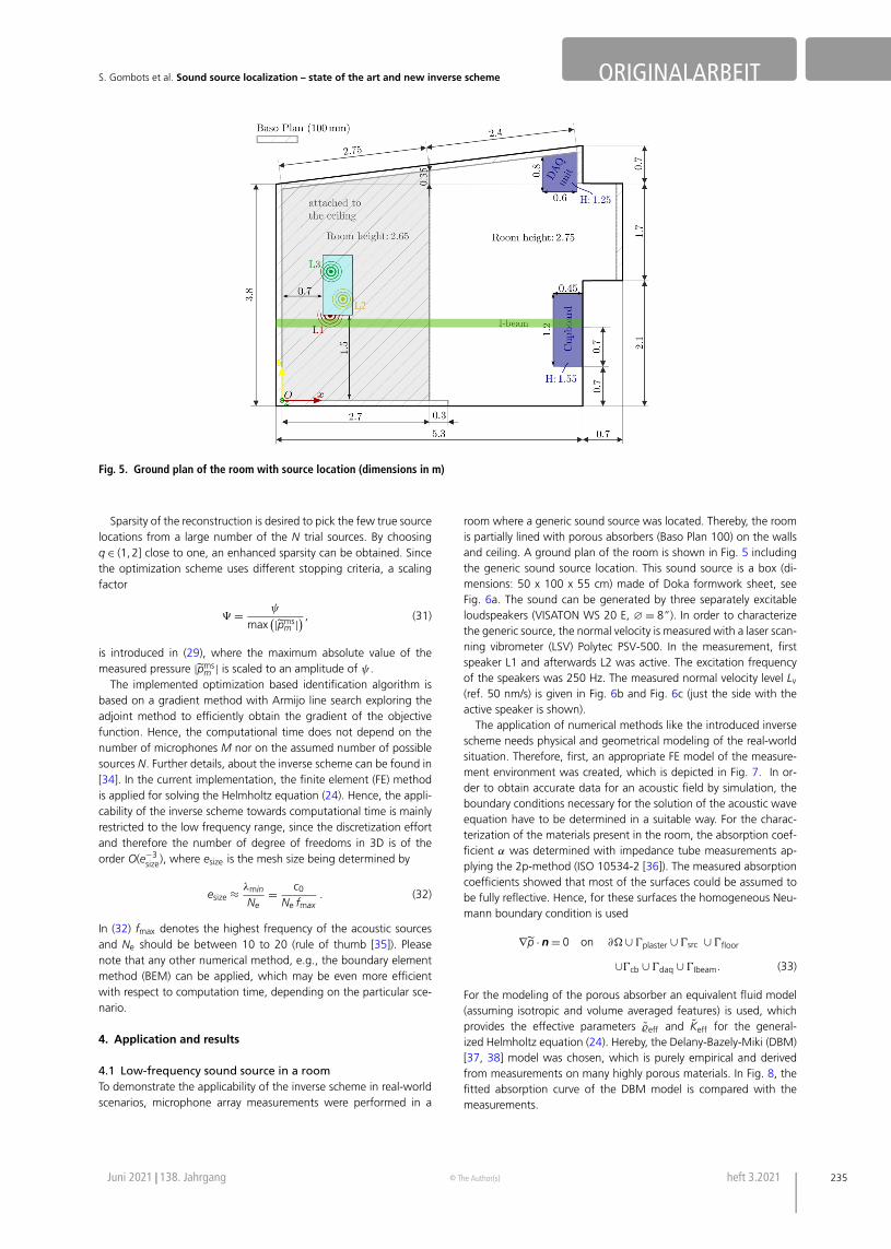
Fig. 5. Ground plan of the room with source location (dimensions in m)

Sparsity of the reconstruction is desired to pick the few true sourcelocations from a large number of the N trial sources. By choosingq ∈ (1, 2] close to one, an enhanced sparsity can be obtained. Sincethe optimization scheme uses different stopping criteria, a scalingfactor

� = ψ

max(|̃pms

m |) , (31)

is introduced in (29), where the maximum absolute value of themeasured pressure |̃pms

m | is scaled to an amplitude of ψ .The implemented optimization based identification algorithm is

based on a gradient method with Armijo line search exploring theadjoint method to efficiently obtain the gradient of the objectivefunction. Hence, the computational time does not depend on thenumber of microphones M nor on the assumed number of possiblesources N. Further details, about the inverse scheme can be found in[34]. In the current implementation, the finite element (FE) methodis applied for solving the Helmholtz equation (24). Hence, the appli-cability of the inverse scheme towards computational time is mainlyrestricted to the low frequency range, since the discretization effortand therefore the number of degree of freedoms in 3D is of theorder O(e−3

size), where esize is the mesh size being determined by

esize ≈ λmin

Ne= c0

Ne fmax. (32)

In (32) fmax denotes the highest frequency of the acoustic sourcesand Ne should be between 10 to 20 (rule of thumb [35]). Pleasenote that any other numerical method, e.g., the boundary elementmethod (BEM) can be applied, which may be even more efficientwith respect to computation time, depending on the particular sce-nario.

4. Application and results

4.1 Low-frequency sound source in a roomTo demonstrate the applicability of the inverse scheme in real-worldscenarios, microphone array measurements were performed in a

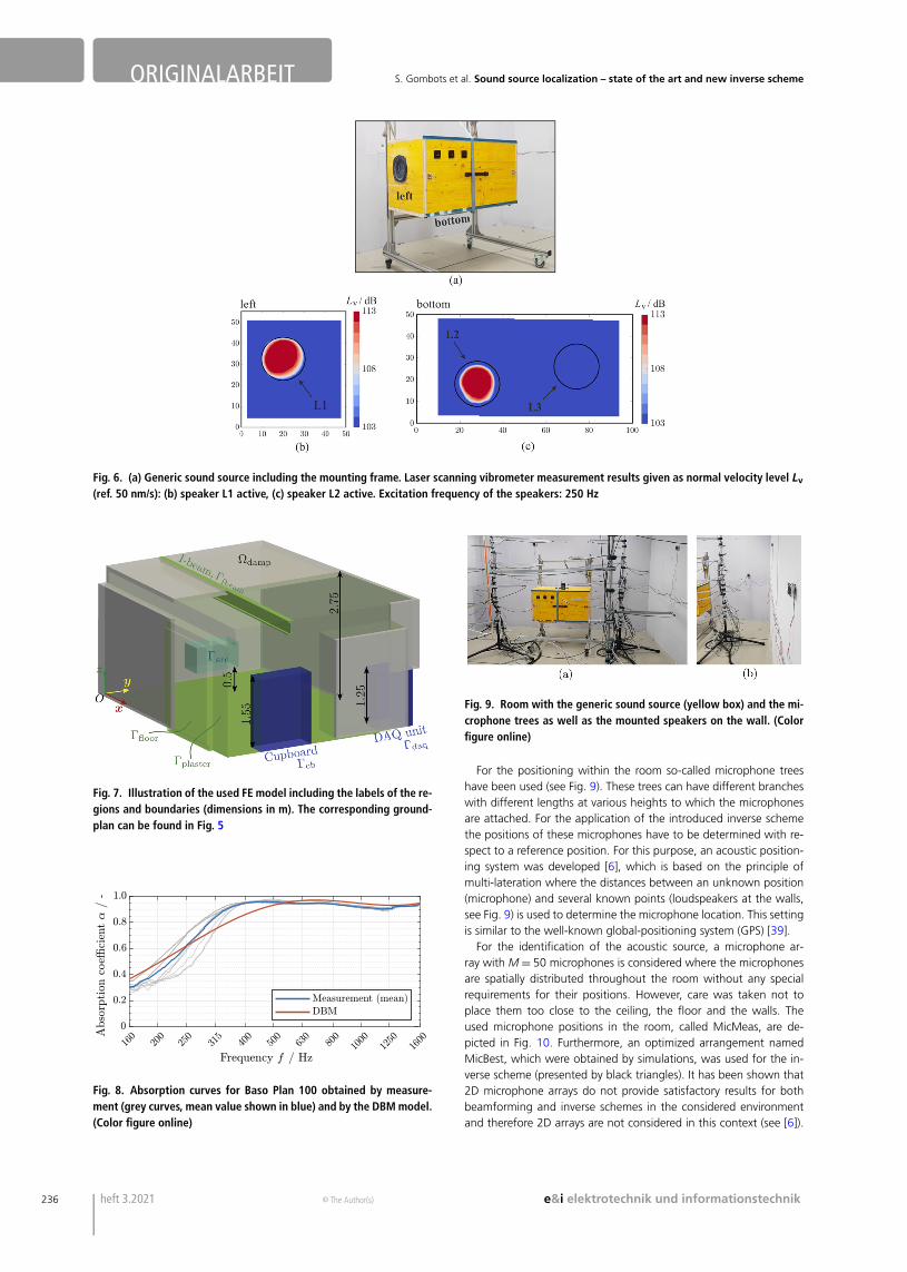
room where a generic sound source was located. Thereby, the roomis partially lined with porous absorbers (Baso Plan 100) on the wallsand ceiling. A ground plan of the room is shown in Fig. 5 includingthe generic sound source location. This sound source is a box (di-mensions: 50 x 100 x 55 cm) made of Doka formwork sheet, seeFig. 6a. The sound can be generated by three separately excitableloudspeakers (VISATON WS 20 E, ∅ = 8”). In order to characterizethe generic source, the normal velocity is measured with a laser scan-ning vibrometer (LSV) Polytec PSV-500. In the measurement, firstspeaker L1 and afterwards L2 was active. The excitation frequencyof the speakers was 250 Hz. The measured normal velocity level Lv

(ref. 50 nm/s) is given in Fig. 6b and Fig. 6c (just the side with theactive speaker is shown).

The application of numerical methods like the introduced inversescheme needs physical and geometrical modeling of the real-worldsituation. Therefore, first, an appropriate FE model of the measure-ment environment was created, which is depicted in Fig. 7. In or-der to obtain accurate data for an acoustic field by simulation, theboundary conditions necessary for the solution of the acoustic waveequation have to be determined in a suitable way. For the charac-terization of the materials present in the room, the absorption coef-ficient α was determined with impedance tube measurements ap-plying the 2p-method (ISO 10534-2 [36]). The measured absorptioncoefficients showed that most of the surfaces could be assumed tobe fully reflective. Hence, for these surfaces the homogeneous Neu-mann boundary condition is used

∇p̃ · n = 0 on ∂� ∪ �plaster ∪ �src ∪ �floor

∪�cb ∪ �daq ∪ �Ibeam. (33)

For the modeling of the porous absorber an equivalent fluid model(assuming isotropic and volume averaged features) is used, whichprovides the effective parameters �̃eff and K̃eff for the general-ized Helmholtz equation (24). Hereby, the Delany-Bazely-Miki (DBM)[37, 38] model was chosen, which is purely empirical and derivedfrom measurements on many highly porous materials. In Fig. 8, thefitted absorption curve of the DBM model is compared with themeasurements.



Fig. 6. (a) Generic sound source including the mounting frame. Laser scanning vibrometer measurement results given as normal velocity level Lv

(ref. 50 nm/s): (b) speaker L1 active, (c) speaker L2 active. Excitation frequency of the speakers: 250 Hz

Fig. 7. Illustration of the used FE model including the labels of the re-gions and boundaries (dimensions in m). The corresponding ground-plan can be found in Fig. 5

Fig. 8. Absorption curves for Baso Plan 100 obtained by measure-ment (grey curves, mean value shown in blue) and by the DBM model.(Color figure online)

Fig. 9. Room with the generic sound source (yellow box) and the mi-crophone trees as well as the mounted speakers on the wall. (Colorfigure online)

For the positioning within the room so-called microphone treeshave been used (see Fig. 9). These trees can have different brancheswith different lengths at various heights to which the microphonesare attached. For the application of the introduced inverse schemethe positions of these microphones have to be determined with re-spect to a reference position. For this purpose, an acoustic position-ing system was developed [6], which is based on the principle ofmulti-lateration where the distances between an unknown position(microphone) and several known points (loudspeakers at the walls,see Fig. 9) is used to determine the microphone location. This settingis similar to the well-known global-positioning system (GPS) [39].

For the identification of the acoustic source, a microphone ar-ray with M = 50 microphones is considered where the microphonesare spatially distributed throughout the room without any specialrequirements for their positions. However, care was taken not toplace them too close to the ceiling, the floor and the walls. Theused microphone positions in the room, called MicMeas, are de-picted in Fig. 10. Furthermore, an optimized arrangement namedMicBest, which were obtained by simulations, was used for the in-verse scheme (presented by black triangles). It has been shown that2D microphone arrays do not provide satisfactory results for bothbeamforming and inverse schemes in the considered environmentand therefore 2D arrays are not considered in this context (see [6]).



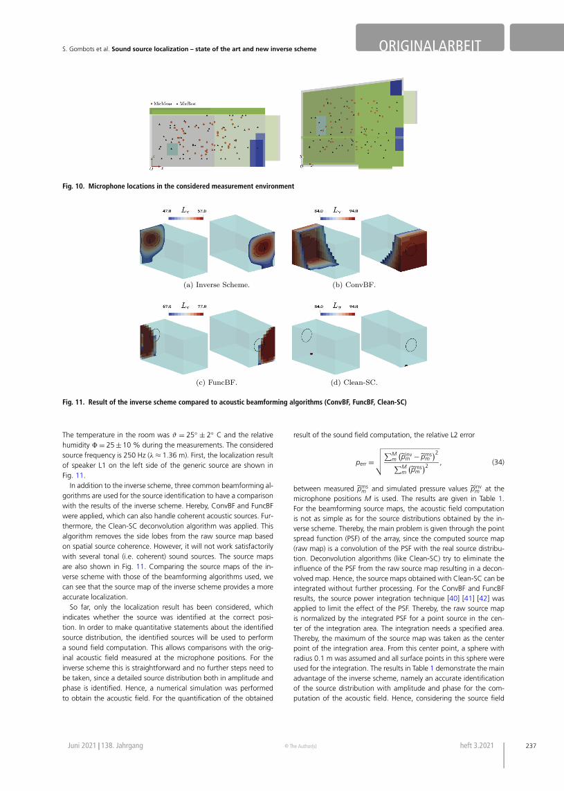
Fig. 10. Microphone locations in the considered measurement environment

Fig. 11. Result of the inverse scheme compared to acoustic beamforming algorithms (ConvBF, FuncBF, Clean-SC)

The temperature in the room was ϑ = 25◦ ± 2◦ C and the relativehumidity � = 25 ± 10 % during the measurements. The consideredsource frequency is 250 Hz (λ ≈ 1.36 m). First, the localization resultof speaker L1 on the left side of the generic source are shown inFig. 11.

In addition to the inverse scheme, three common beamforming al-gorithms are used for the source identification to have a comparisonwith the results of the inverse scheme. Hereby, ConvBF and FuncBFwere applied, which can also handle coherent acoustic sources. Fur-thermore, the Clean-SC deconvolution algorithm was applied. Thisalgorithm removes the side lobes from the raw source map basedon spatial source coherence. However, it will not work satisfactorilywith several tonal (i.e. coherent) sound sources. The source mapsare also shown in Fig. 11. Comparing the source maps of the in-verse scheme with those of the beamforming algorithms used, wecan see that the source map of the inverse scheme provides a moreaccurate localization.

So far, only the localization result has been considered, whichindicates whether the source was identified at the correct posi-tion. In order to make quantitative statements about the identifiedsource distribution, the identified sources will be used to performa sound field computation. This allows comparisons with the orig-inal acoustic field measured at the microphone positions. For theinverse scheme this is straightforward and no further steps need tobe taken, since a detailed source distribution both in amplitude andphase is identified. Hence, a numerical simulation was performedto obtain the acoustic field. For the quantification of the obtained

result of the sound field computation, the relative L2 error

perr =√

√

√

√

∑Mm

(

p̃invm − p̃ms

m)2

∑Mm

(

p̃msm

)2, (34)

between measured p̃msm and simulated pressure values p̃inv

m at themicrophone positions M is used. The results are given in Table 1.For the beamforming source maps, the acoustic field computationis not as simple as for the source distributions obtained by the in-verse scheme. Thereby, the main problem is given through the pointspread function (PSF) of the array, since the computed source map(raw map) is a convolution of the PSF with the real source distribu-tion. Deconvolution algorithms (like Clean-SC) try to eliminate theinfluence of the PSF from the raw source map resulting in a decon-volved map. Hence, the source maps obtained with Clean-SC can beintegrated without further processing. For the ConvBF and FuncBFresults, the source power integration technique [40] [41] [42] wasapplied to limit the effect of the PSF. Thereby, the raw source mapis normalized by the integrated PSF for a point source in the cen-ter of the integration area. The integration needs a specified area.Thereby, the maximum of the source map was taken as the centerpoint of the integration area. From this center point, a sphere withradius 0.1 m was assumed and all surface points in this sphere wereused for the integration. The results in Table 1 demonstrate the mainadvantage of the inverse scheme, namely an accurate identificationof the source distribution with amplitude and phase for the com-putation of the acoustic field. Hence, considering the source field



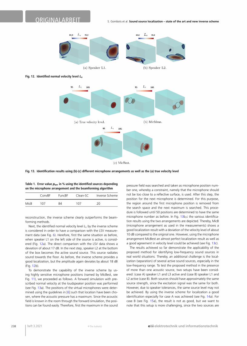
Fig. 12. Identified normal velocity level Lv

Fig. 13. Identification results using (b)-(c) different microphone arrangements as well as the (a) true velocity level

Table 1. Error value perr in % using the identified sources dependingon the microphone arrangement and the beamforming algorithm

ConvBF FuncBF Clean-SC Inverse Scheme

MicB 107 84 107 20

reconstruction, the inverse scheme clearly outperforms the beam-forming methods.

Next, the identified normal velocity level Lv by the inverse schemeis considered in order to have a comparison with the LSV measure-ment data (see Fig. 6). Herefore, first the same situation as before,when speaker L1 on the left side of the source is active, is consid-ered (Fig. 12a). The direct comparison with the LSV data shows adeviation of about 17 dB. In the next step, speaker L2 at the bottomof the box becomes the active sound source. This source radiatessound towards the floor. As before, the inverse scheme provides agood localization, but the amplitude again deviates by about 18 dB(Fig. 12b).

To demonstrate the capability of the inverse scheme by us-ing highly sensitive microphone positions (named by MicBest, seeFig. 11), we proceeded as follows. A forward simulation with pre-scribed normal velocity at the loudspeaker position was performed(see Fig. 13a). The positions of the virtual microphones were deter-mined using the guidelines in [6] such that location have been cho-sen, where the acoustic pressure has a maximum. Since the acousticfield is known in the room through the forward simulation, the posi-tions can be found easily. Therefore, first the maximum in the sound

pressure field was searched and taken as microphone position num-ber one, whereby a constraint, namely that the microphone shouldnot be too close to a reflective surface, is used. After this step, theposition for the next microphone is determined. For this purpose,the region around the first microphone position is removed fromthe search space and the next maximum is searched. This proce-dure is followed until 50 positions are determined to have the samemicrophone number as before. In Fig. 13b,c the various identifica-tion results using the two arrangements are depicted. Thereby, MicB(microphone arrangement as used in the measurements) shows agood localization result with a deviation of the velocity level of about10 dB compared to the original one. However, using the microphonearrangement MicBest an almost perfect localization result as well asa good agreement in velocity level could be achieved (see Fig. 13c).

The results achieved so far demonstrate the applicability of theproposed method for identifying low-frequency sound sources inreal world situations. Thereby, an additional challenge is the local-ization (separation) of several active sound sources, especially in thelow-frequency range. To test the proposed method in the presenceof more than one acoustic source, two setups have been consid-ered: (case A) speaker L1 and L3 active and (case B) speaker L1 andL2 active (case B). Both sources should have approximately the samesource strength, since the excitation signal was the same for both.However, due to speaker tolerances, the same source level may notbe achieved. By using the inverse scheme for localization a goodidentification especially for case A was achieved (see Fig. 14a). Forcase B (see Fig. 15a), the result is not as good, but we want tonote that this setup is more challenging, since the two sources are



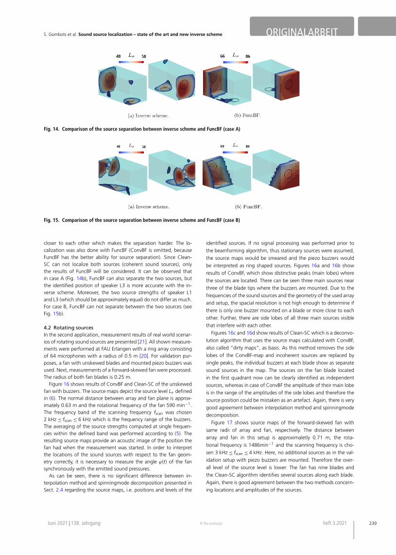
Fig. 14. Comparison of the source separation between inverse scheme and FuncBF (case A)

Fig. 15. Comparison of the source separation between inverse scheme and FuncBF (case B)

closer to each other which makes the separation harder. The lo-calization was also done with FuncBF (ConvBF is omitted, becauseFuncBF has the better ability for source separation). Since Clean-SC can not localize both sources (coherent sound sources), onlythe results of FuncBF will be considered. It can be observed thatin case A (Fig. 14b), FuncBF can also separate the two sources, butthe identified position of speaker L3 is more accurate with the in-verse scheme. Moreover, the two source strengths of speaker L1and L3 (which should be approximately equal) do not differ as much.For case B, FuncBF can not separate between the two sources (seeFig. 15b).

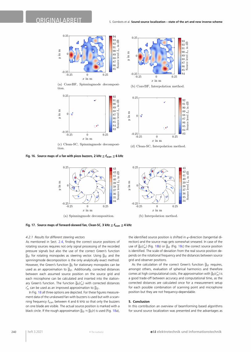
4.2 Rotating sourcesIn the second application, measurement results of real world scenar-ios of rotating sound sources are presented [21]. All shown measure-ments were performed at FAU Erlangen with a ring array consistingof 64 microphones with a radius of 0.5 m [20]. For validation pur-poses, a fan with unskewed blades and mounted piezo buzzers wasused. Next, measurements of a forward-skewed fan were processed.The radius of both fan blades is 0.25 m.

Figure 16 shows results of ConvBF and Clean-SC of the unskewedfan with buzzers. The source maps depict the source level Lσ definedin (6). The normal distance between array and fan plane is approx-imately 0.63 m and the rotational frequency of the fan 590 min−1.The frequency band of the scanning frequency fscan was chosen2 kHz ≤ fscan ≤ 6 kHz which is the frequency range of the buzzers.The averaging of the source strengths computed at single frequen-cies within the defined band was performed according to (5). Theresulting source maps provide an acoustic image of the position thefan had when the measurement was started. In order to interpretthe locations of the sound sources with respect to the fan geom-etry correctly, it is necessary to measure the angle ϕ(t) of the fansynchronously with the emitted sound pressures.

As can be seen, there is no significant difference between in-terpolation method and spinningmode decomposition presented inSect. 2.4 regarding the source maps, i.e. positions and levels of the

identified sources. If no signal processing was performed prior to

the beamforming algorithm, thus stationary sources were assumed,

the source maps would be smeared and the piezo buzzers would

be interpreted as ring shaped sources. Figures 16a and 16b show

results of ConvBF, which show distinctive peaks (main lobes) where

the sources are located. There can be seen three main sources near

three of the blade tips where the buzzers are mounted. Due to the

frequencies of the sound sources and the geometry of the used array

and setup, the spacial resolution is not high enough to determine if

there is only one buzzer mounted on a blade or more close to each

other. Further, there are side lobes of all three main sources visible

that interfere with each other.

Figures 16c and 16d show results of Clean-SC which is a deconvo-

lution algorithm that uses the source maps calculated with ConvBF,

also called “dirty maps”, as basis. As this method removes the side

lobes of the ConvBF-map and incoherent sources are replaced by

single peaks, the individual buzzers at each blade show as separate

sound sources in the map. The sources on the fan blade located

in the first quadrant now can be clearly identified as independent

sources, whereas in case of ConvBF the amplitude of their main lobe

is in the range of the amplitudes of the side lobes and therefore the

source position could be mistaken as an artefact. Again, there is very

good agreement between interpolation method and spinningmode

decomposition.

Figure 17 shows source maps of the forward-skewed fan with

same radii of array and fan, respectively. The distance between

array and fan in this setup is approximaletly 0.71 m, the rota-

tional frequency is 1486min−1 and the scanning frequency is cho-

sen 3 kHz ≤ fscan ≤ 4 kHz. Here, no additional sources as in the val-

idation setup with piezo buzzers are mounted. Therefore the over-

all level of the source level is lower. The fan has nine blades and

the Clean-SC algorithm identifies several sources along each blade.

Again, there is good agreement between the two methods concern-

ing locations and amplitudes of the sources.



Fig. 16. Source maps of a fan with piezo buzzers, 2 kHz ≤ fscan ≤ 6 kHz

Fig. 17. Source maps of forward-skewed fan, Clean-SC, 3 kHz ≤ fscan ≤ 4 kHz

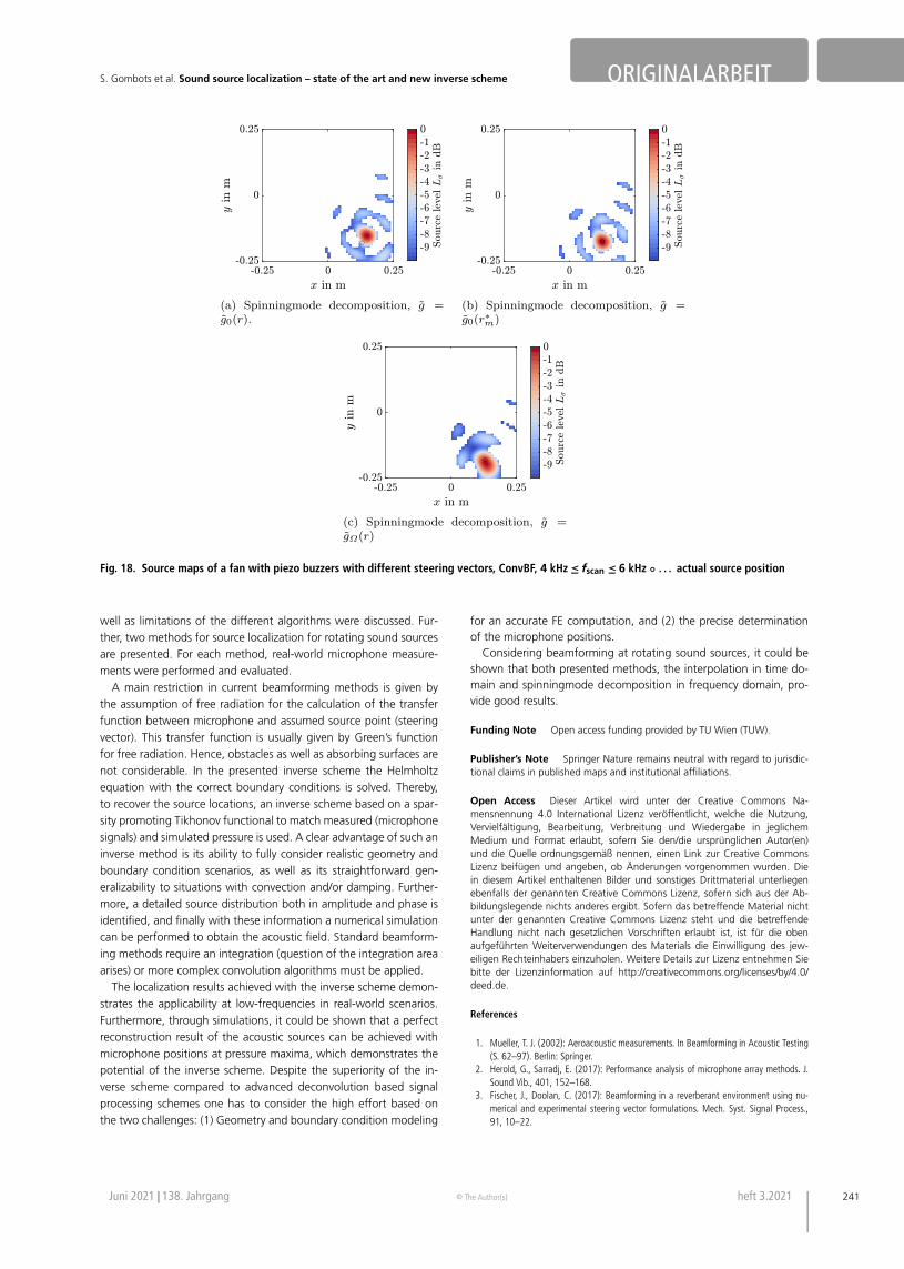
4.2.1 Results for different steering vectorsAs mentioned in Sect. 2.4, finding the correct source positions ofrotating sources requires not only signal processing of the recordedpressure signals but also the use of the correct Green’s functiong̃Ω for rotating monopoles as steering vector. Using g̃Ω and thespinningmode decomposition is the only analytically exact method.However, the Green’s function g̃0 for stationary monopoles can beused as an approximation to g̃Ω . Additionally, corrected distancesbetween each assumed source position on the source grid andeach microphone can be calculated and inserted into the station-ary Green’s function. The function g̃0(r*

m) with corrected distancesr*m can be used as an improved approximation to g̃Ω .

In Fig. 18 all three options are depicted. For these figures measure-ment data of the unskewed fan with buzzers is used but with a scan-ning frequency fscan between 4 and 6 kHz so that only the buzzerson one blade are visible. The actual source position is marked with ablack circle. If the rough approximation g̃Ω ≈ g̃0(r) is used (Fig. 18a),

the identified source position is shifted in ϕ-direction (tangential di-rection) and the source map gets somewhat smeared. In case of theuse of g̃0(r*

m) (Fig. 18b) or g̃Ω (Fig. 18c) the correct source positionis identified. The scale of deviation from the real source position de-pends on the rotational frequency and the distances between sourcegrid and observer positions.

As the calculation of the correct Green’s function g̃Ω requires,amongst others, evaluation of spherical harmonics and thereforecomes at high computational costs, the approximation with g̃0(r*

m) isa good trade-off between accuracy and computational time, as thecorrected distances are calculated once for a measurement setupfor each possible combination of scanning point and microphoneposition but they are not frequency-dependable.

5. ConclusionIn this contribution an overview of beamforming based algorithmsfor sound source localization was presented and the advantages as



Fig. 18. Source maps of a fan with piezo buzzers with different steering vectors, ConvBF, 4 kHz ≤ fscan ≤ 6 kHz ◦ . . . actual source position

well as limitations of the different algorithms were discussed. Fur-ther, two methods for source localization for rotating sound sourcesare presented. For each method, real-world microphone measure-ments were performed and evaluated.

A main restriction in current beamforming methods is given bythe assumption of free radiation for the calculation of the transferfunction between microphone and assumed source point (steeringvector). This transfer function is usually given by Green’s functionfor free radiation. Hence, obstacles as well as absorbing surfaces arenot considerable. In the presented inverse scheme the Helmholtzequation with the correct boundary conditions is solved. Thereby,to recover the source locations, an inverse scheme based on a spar-sity promoting Tikhonov functional to match measured (microphonesignals) and simulated pressure is used. A clear advantage of such aninverse method is its ability to fully consider realistic geometry andboundary condition scenarios, as well as its straightforward gen-eralizability to situations with convection and/or damping. Further-more, a detailed source distribution both in amplitude and phase isidentified, and finally with these information a numerical simulationcan be performed to obtain the acoustic field. Standard beamform-ing methods require an integration (question of the integration areaarises) or more complex convolution algorithms must be applied.

The localization results achieved with the inverse scheme demon-strates the applicability at low-frequencies in real-world scenarios.Furthermore, through simulations, it could be shown that a perfectreconstruction result of the acoustic sources can be achieved withmicrophone positions at pressure maxima, which demonstrates thepotential of the inverse scheme. Despite the superiority of the in-verse scheme compared to advanced deconvolution based signalprocessing schemes one has to consider the high effort based onthe two challenges: (1) Geometry and boundary condition modeling

for an accurate FE computation, and (2) the precise determinationof the microphone positions.

Considering beamforming at rotating sound sources, it could beshown that both presented methods, the interpolation in time do-main and spinningmode decomposition in frequency domain, pro-vide good results.

Funding Note Open access funding provided by TU Wien (TUW).

Publisher’s Note Springer Nature remains neutral with regard to jurisdic-tional claims in published maps and institutional affiliations.

Open Access Dieser Artikel wird unter der Creative Commons Na-mensnennung 4.0 International Lizenz veröffentlicht, welche die Nutzung,Vervielfältigung, Bearbeitung, Verbreitung und Wiedergabe in jeglichemMedium und Format erlaubt, sofern Sie den/die ursprünglichen Autor(en)und die Quelle ordnungsgemäß nennen, einen Link zur Creative CommonsLizenz beifügen und angeben, ob Änderungen vorgenommen wurden. Diein diesem Artikel enthaltenen Bilder und sonstiges Drittmaterial unterliegenebenfalls der genannten Creative Commons Lizenz, sofern sich aus der Ab-bildungslegende nichts anderes ergibt. Sofern das betreffende Material nichtunter der genannten Creative Commons Lizenz steht und die betreffendeHandlung nicht nach gesetzlichen Vorschriften erlaubt ist, ist für die obenaufgeführten Weiterverwendungen des Materials die Einwilligung des jew-eiligen Rechteinhabers einzuholen. Weitere Details zur Lizenz entnehmen Siebitte der Lizenzinformation auf http://creativecommons.org/licenses/by/4.0/deed.de.

References

1. Mueller, T. J. (2002): Aeroacoustic measurements. In Beamforming in Acoustic Testing(S. 62–97). Berlin: Springer.

2. Herold, G., Sarradj, E. (2017): Performance analysis of microphone array methods. J.Sound Vib., 401, 152–168.

3. Fischer, J., Doolan, C. (2017): Beamforming in a reverberant environment using nu-merical and experimental steering vector formulations. Mech. Syst. Signal Process.,91, 10–22.



4. Sarradj, E. (2012): Three-dimensional acoustic sourcemapping with different beam-forming steering vector formulations. Adv. Acoust. Vib., 2012, 292695.

5. Gombots, S., Kaltenbacher, M., Kaltenbacher, B. (2016): Combined Experimental-Simulation Based Acoustic Source Localization, Fortschritte der Akustik. DAGA 2016.Deut. Jahrestagung Akust., 42, 1092–1095.

6. Gombots, S. (2020): Acoustic source localization at low frequencies using microphonearrays. PhD Thesis, TU Wien.

7. Dougherty, R., Walker, B. (2009): Virtual Rotating Microphone Imaging of BroadbandFan Noise, 15th AIAA/CEAS Aeroacoustics Conference (30th AIAA Aeroacoustics Con-ference). AIAA 2009-3121.

8. Johnson, D. H., Dudgeon, D. E. (1993): Array signal processing: concepts and tech-niques. In Finite Continuous Apertures (S. 64–65). Englewood Cliffs: PTR PrenticeHall.

9. Dougherty, R. P., Ramachandran, R. C., Raman, G. (2013): Deconvolution of sourcesin aeroacoustic images from phased microphone arrays using linear programming. Int.J. Aeroacoust., 12(7–8), 699–717.

10. Dougherty, R. P. (2014): Functional Beamforming. In 5th Berlin Beamforming Confer-ence. BeBeC-2014-01.

11. Dougherty, R. P. (2014): Functional Beamforming for Aeroacoustic Source Distribu-tions, 20th AIAA/CEAS Aeroacoustics Conference. AIAA 2014-3066.

12. Brooks, T. F., Humphreys, W. M. (2006): A deconvolution approach for the mapping ofacoustic sources (damas) determined from phased microphone arrays. J. Sound Vib.,294, 856–879.

13. Sijtsma, P. (2007): CLEAN based on spatial source coherence. Int. J. Aeroacoust., 6(4),357–374.

14. Yardibi, T., Li, J., Stoica, P., Cattafesta, L. N. (2008): Sparsity constrained deconvolutionapproaches for acoustic source mapping. J. Acoust. Soc. Am., 123(5), 2631–2642.

15. Chu, Z., Yang, Y. (2014): Comparison of deconvolution methods for the visualization ofacoustic sources based on cross-spectral imaging function beamforming. Mech. Syst.Signal Poces., 48(3), 404–422.

16. Padois, T., Berry, A. (2017): Two and Three-Dimensional Sound Source Localizationwith Beamforming and Several Deconvolution Techniques. Acta Acust. Acust., 103(3),357–392.

17. Dowling, A. P., Ffowcs, W. J. (1983): Sound and sources of sound. Chichester: E. Hor-wood. 1983.

18. Herold, G., Sarradj, E. (2015): Microphone array method for the characterization ofrotating sound sources in axial fans. Noise Control Eng. J., 63, 546–551.

19. Dougherty, R., Walker, B. (2009): Virtual Rotating Microphone Imaging of BroadbandFan Noise., 15th AIAA/CEAS Aeroacoustics Conference (30th AIAA AeroacousticsConference). Aeroacoustics Conferences. Washington: AIAA.

20. Krömer, F. (2018): Sound emission of low-pressure axial fans under distorted inflowconditions, FAU Forschungen, Reihe B, Medizin. Naturwissenschaft, Technik.

21. Nowak, J., Krömer, F., Kaltenbacher, M. (2019): Vergleich verschiedener Methoden zurSchallquellenlokalisation bei Axialventilatoren, Fortschritte der Akustik. DAGA 2019.Deut. Jahrestagung Akust., 45, 31–34. 2019.

22. Sarradj, E. (2008): Quantitative source spectra from acoustic array measurements. In2nd Berlin Beamforming Conference. BeBeC-2008-03.

23. Sarradj, E., Geyer, T., Brick, H., Kirchner, K.-R., Kohrs, T. (2012): In Application of Beam-forming and Deconvolution Techniques to Aeroacoustic Sources at Highspeed Trains,NOVEM – Noise and Vibration: Emerging Methods, Sorrento.

24. Merino-Martínez, R., Sijtsma, P., Carpio, A. R., Zamponi, R., Luesutthiviboon, S., Mal-goezar, A. M. N., Snellen, M., Schram, C., Simons, D. G. (2019): Integration methodsfor distributed sound sources. Int. J. Aeroacoust., 18(4–5), 444–469.

25. Leclere, Q., Pereira, A., Bailly, C., Antoni, J., Picard, C. (2017): A unified formalism foracoustic imaging based on microphone array measurements. Int. J. Aeroacoust., 16,431–456.

26. Ehrenfried, K., Koop, L. (2007): Comparison of Iterative Deconvolution Algorithms forthe Mapping of Acoustic Sources. AIAA J., 45(7), 1584–1595.

27. Yardibi, T., Zawodny, N. S., Bahr, C., Liu, F., Cattafesta, L. N., Li, J. (2010): Comparisonof Microphone Array Processing Techniques for Aeroacoustic Measurements. Int. J.Aeroacoust., 9(6), 733–761.

28. Merino-Martínez, R., Sijtsma, P., Snellen, M., Ahlefeldt, T., Bahr, C. J., Blacodon, D.,Ernst, D., Finez, A., Funke, S., Geyer, T. F., Haxter, S., Herold, G., Huang, X., HumphreysWIllam, W. M., Leclère, Q., Malgoezar, A., Michel, U., Padois, T., Pereira, A., Picard, C.,Sarradj, E., Siller, H., Simons, D. G., Spehr, C. (2019): A Review of Acoustic ImagingMethods Using Phased Microphone Arrays. CEAS Aeronaut. J., 10, 197–230.

29. Chiariotti, P., Martarelli, M., Castellini, P. (2019): Acoustic beamforming for noisesource localization: Reviews, methodology and applications. Mech. Syst. Signal Pro-cess., 120, 422–448.

30. Suzuki, T. (2011): L1 generalized inverse beam-forming algorithm resolving coher-ent/incoherent, distributed and multipole sources. J. Sound Vib., 330, 5835–5851.

31. Deckers, E., Jonckheere, S., Vandepitte, D., Desmet, W. (2015): Modelling techniquesfor vibro-acoustic dynamics of poroelastic materials. Arch. Comput. Methods Eng.,22(2), 183–236.

32. Anzengruber, S. W., Hofmann, B., Mathé, P. (2014): Regularization properties of thesequential discrepancy principle for Tikhonov regularization in Banach spaces. Appl.Anal., 93(7), 1382–1400.

33. Lu, S., Pereverzev, S. V. (2011): Multi-parameter regularization and its numerical real-ization. Numer. Math., 118(1), 1–31.

34. Kaltenbacher, M., Kaltenbacher, B., Gombots, S. (2018): Inverse Scheme for AcousticSource Localization using Microphone Measurements and Finite Element Simulations.Acta Acust. Acust., 104, 647–656.

35. Kaltenbacher, M. (2015): Numerical Simulation of Mechatronic Sensors and Actuators:Finite Elements for Computational Multiphysics. 3. ed. Berlin: Springer.

36. ISO 10534-2 (2001): Acoustics – Determination of sound absorption coefficient andimpedance in impedance tubes – Part 2: Transfer-function method.

37. Delany, M. E., Bazley, E. N. (1970): Acoustical properties of fibrous absorbent materi-als. Appl. Acoust., 3(2), 105–116.

38. Delany, M. E., Bazley, E. N. (1990): Acoustical properties of porous materials. Modifi-cations of Delany-Bazley models. J. Acoust. Soc. Jpn., 11(1), 19–24.

39. Hofmann-Wellenhof, B., Lichtenegger, H., Collins, J. (2012): Global positioning system:theory and practice. Berlin: Springer.

40. Brooks, T. F., Humphreys, W. M. (1999): Effect of directional array size on the mea-surement of airframe noise components. In 5th AIAA/CEAS Aeroacoustics Conferenceand Exhibit (S. 99–1958). Washington: AIAA.

41. Sijtsma, P. (2010): Phased Array Beamforming Applied to Wind Tunnel And Fly-OverTests. SAE Brasil International Noise and Vibration Congress. SAE International.

42. Merino-Martínez, R., Neri, E., Snellen, M., Kennedy, J., Simons, D., Bennett, G. J.(2017): Comparing flyover noise measurements to full-scale nose landing gear windtunnel experiments for regional aircraft. In 23rd AIAA/CEAS Aeroacoustics Conference.AIAA 2017-3006.

Authors

Stefan Gombotsgraduated in Mechanical Engineering fromTU Wien in 2015 and received his PhD fromTU Wien in 2020. His research focuses onsound source localization utilizing acousticmeasurements and simulations.

Jonathan Nowakgraduated from TU Wien in 2018 with a mas-ters degree in Mechanical Engineering – Eco-nomics. The topic of his master thesis wassound source localization of rotating sources.Since 2018 he has been working under thesupervision of Prof. Manfred Kaltenbacher asa university assistant at the Institute of Me-chanics and Mechatronics at TU Wien in theresearch unit of Technical Acoustics. His main

research topic is sound source localization using microphone mea-surements and the Finite Element method. His teaching responsibil-ities invlove the exam and exercise of Measurement and VibrationTechnology.



Manfred Kaltenbacherreceived his Dipl.-Ing. in electrical engineer-ing from the Technical University of Graz,Austria in 1992, his Ph.D. in technical sciencefrom the Johannes Kepler University of Linz,Austria in 1996, and his habilitation fromFriedrich-Alexander-University of Erlangen-Nuremberg, Germany, in 2004. In 2008 hebecame a full professor for Applied Mecha-tronics at Alps-Adriatic University Klagenfurt,

Austria. In 2012 he moved to TU Wien, Austria, as a full professorfor Measurement and Actuator Technology, and in 2020 he becamethe head of the Institute of Fundamentals and Theory in ElectricalEngineering at TU Graz, Austria. His research involves theory, mod-eling, simulation and experimental investigation of complex systemsin engineering, material and medical science. A main focus is on thedevelopment of advanced Finite Element (FE) methods for multi-fieldproblems (electromagnetics-mechanics, mechanics-acoustics, piezo-electricity, flow dynamics – mechanics, aeroacoustics), and their ap-plication to design mechatronic sensors and actuators.


Documents

Sound source localization – state of the art and new