Sound radiation of a ba†ed plate; theoretical and ... · PDF file2.2 Boundary Element Method ... together with SYSNOISE for ... total radiated sound power normalized with respect

Sound radiation of a baffled plate;theoretical and numerical approach

A.J. van Engelen

DCT 2009.005

Research report

Supervisor: Dr.ir. I. Lopez

Eindhoven University of TechnologyDepartment of Mechanical EngineeringDynamics and Control Group

Eindhoven, January 2009

ii

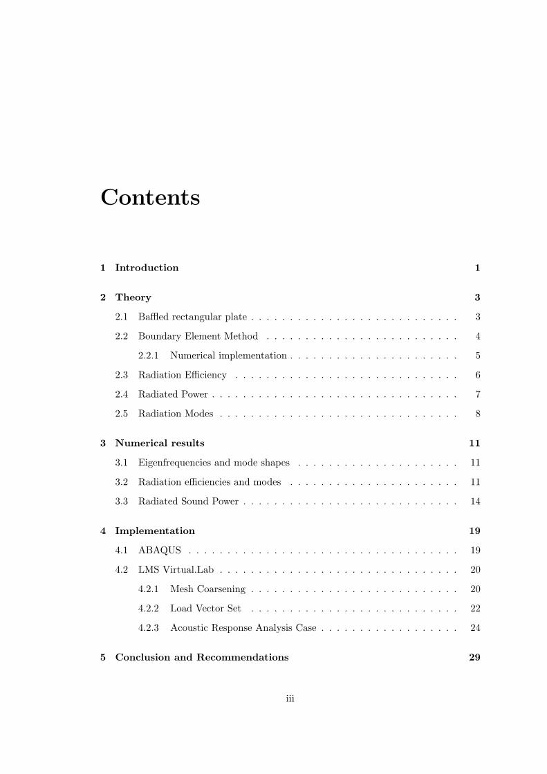
Contents

1 Introduction 1

2 Theory 3

2.1 Baffled rectangular plate . . . . . . . . . . . . . . . . . . . . . . . . . . . 3

2.2 Boundary Element Method . . . . . . . . . . . . . . . . . . . . . . . . . 4

2.2.1 Numerical implementation . . . . . . . . . . . . . . . . . . . . . . 5

2.3 Radiation Efficiency . . . . . . . . . . . . . . . . . . . . . . . . . . . . . 6

2.4 Radiated Power . . . . . . . . . . . . . . . . . . . . . . . . . . . . . . . . 7

2.5 Radiation Modes . . . . . . . . . . . . . . . . . . . . . . . . . . . . . . . 8

3 Numerical results 11

3.1 Eigenfrequencies and mode shapes . . . . . . . . . . . . . . . . . . . . . 11

3.2 Radiation efficiencies and modes . . . . . . . . . . . . . . . . . . . . . . 11

3.3 Radiated Sound Power . . . . . . . . . . . . . . . . . . . . . . . . . . . . 14

4 Implementation 19

4.1 ABAQUS . . . . . . . . . . . . . . . . . . . . . . . . . . . . . . . . . . . 19

4.2 LMS Virtual.Lab . . . . . . . . . . . . . . . . . . . . . . . . . . . . . . . 20

4.2.1 Mesh Coarsening . . . . . . . . . . . . . . . . . . . . . . . . . . . 20

4.2.2 Load Vector Set . . . . . . . . . . . . . . . . . . . . . . . . . . . 22

4.2.3 Acoustic Response Analysis Case . . . . . . . . . . . . . . . . . . 24

5 Conclusion and Recommendations 29

iii

iv Contents

Bibliography 31

A ABAQUS input file 33

B Export of BEM matrices 35

Chapter 1

Introduction

Nowadays for manufactures it is of a high importance to produce low noise products.Policies exist to minimize the sound power radiated by machinery, airports and high-ways. Besides these policies set by the government manufactures need to comply withthe demands of the costumor, who often prefer low noise designs. On the other handthere are also products that have to produce sound for functional reasons, for exam-ple a speaker system. For these reasons it is important to understand the behavior ofmechanical structures that produce sound, whether it is functional sound or noise.

To answer the need of manufactures to be able to quantify the sound production of theirproduct on beforehand without the use of a prototype, computer software is developed.With the ever increasing computational power of modern computers more powerfulsoftware is introduced to perform simulations to calculate the radiated sound power ofcomplex structures. Moreover, manufactures are able to integrate the aspect of soundproduction into an early development stage of their product design.

In this report theory about the radiated sound of a baffled rectangular plate is comparedwith simulation results obtained from computer software. In this way conclusions can bedrawn about the accuracy of the model that is used in the simulations. First the theoryabout the structural behavior of a simply supported plate is presented. Secondly sometheory about radiation efficiency and radiation modes are presented. In Chapter 3 thesetheoretical results are compared with the results from the numerical model. Chapter 4will give more insight in the process of modeling, exporting and importing results fromone software package into another one. And finally in Chapter 5 some discussions andrecommendations will be done.

1

2 Chapter 1. Introduction

Chapter 2

Theory

2.1 Baffled rectangular plate

To estimate the radiated sound power by a vibrating structure computer software canbe used. In order to be sure that a correct model is used, the results have to becompared with theory. Theory exist about simple structures like a rectangular plate.Therefore in this report a baffled rectangular plate (without damping) is investigated,see Figure 2.1(a). The plate is simply supported at the edges; there are no translationaldegrees of freedom at the edges, see Figure 2.1(b). Throughout the report the properties,mentioned in Table 2.1, of an aluminium plate are used.

The natural eigenfrequencies and eigenmodes of this simply supported rectangular platecan be calculated. From theory [Fah87] the eigenfrequencies equal

ωr =√

Dm

[(r1πa

)2+

(r2πb

)2], (2.1)

where r1 and r2 are the modal indices of the r-th mode and m and D represent the massper unit area (m = ρh) and the bending stiffness per unit length (D = Eh3/12(1− ν2))respectively. Physically the numbers r1 and r2 represent the number of half sine-wavesin x and y direction of the plate in the corresponding mode shape. In Table 2.2 thefirst 10 eigenfrequencies corresponding with the (r1, r2)-th mode are denoted. Thecorresponding structural mode shapes can be calculated with

Property Symbol Value Property Symbol ValueLength [m] a 0.414 Density [kg/m3] ρ 2700Width [m] b 0.314 Youngs Modulus [GPa] E 71Thickness [mm] h 2.0 Poisson ratio [-] ν 0.33

Table 2.1: Properties of the aluminium plate.

3

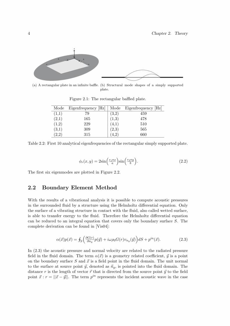
4 Chapter 2. Theory

xy

z

a b

(a) A rectangular plate in an infinite baffle. (b) Structural mode shapes of a simply supportedplate.

Figure 2.1: The rectangular baffled plate.

Mode Eigenfrequency [Hz] Mode Eigenfrequency [Hz](1,1) 79 (3,2) 459(2,1) 165 (1,3) 478(1,2) 229 (4,1) 510(3,1) 309 (2,3) 565(2,2) 315 (4,2) 660

Table 2.2: First 10 analytical eigenfrequencies of the rectangular simply supported plate.

φr(x, y) = 2sin(

r1πxa

)sin

(r2πy

b

). (2.2)

The first six eigenmodes are plotted in Figure 2.2.

2.2 Boundary Element Method

With the results of a vibrational analysis it is possible to compute acoustic pressuresin the surrounded fluid by a structure using the Helmholtz differential equation. Onlythe surface of a vibrating structure in contact with the fluid, also called wetted surface,is able to transfer energy to the fluid. Therefore the Helmholtz differential equationcan be reduced to an integral equation that covers only the boundary surface S. Thecomplete derivation can be found in [Vis04]:

α(~x)p(~x) =∮S

(∂G(r)∂ny

p(~y) + iωρ0G(r)vny(~y))dS + pin(~x). (2.3)

In (2.3) the acoustic pressure and normal velocity are related to the radiated pressurefield in the fluid domain. The term α(~x) is a geometry related coefficient, ~y is a pointon the boundary surface S and ~x is a field point in the fluid domain. The unit normalto the surface at source point ~y, denoted as ~ny, is pointed into the fluid domain. Thedistance r is the length of vector ~r that is directed from the source point ~y to the fieldpoint ~x : r = ||~x − ~y||. The term pin represents the incident acoustic wave in the case

2.2. Boundary Element Method 5

00.05

0.10.15

0.20.25

0.3

0

0.1

0.2

0.3

0.4

−1

−0.5

0

0.5

1

(a) Mode (1,1)

00.05

0.10.15

0.20.25

0.3

0

0.1

0.2

0.3

0.4

−1

−0.5

0

0.5

1

(b) Mode (2,1)

00.05

0.10.15

0.20.25

0.3

0

0.1

0.2

0.3

0.4

−1

−0.5

0

0.5

1

(c) Mode (1,2)

00.05

0.10.15

0.20.25

0.3

0

0.1

0.2

0.3

0.4

−1

−0.5

0

0.5

1

(d) Mode (3,1)

00.05

0.10.15

0.20.25

0.3

0

0.1

0.2

0.3

0.4

−1

−0.5

0

0.5

1

(e) Mode (2,2)

00.05

0.10.15

0.20.25

0.3

0

0.1

0.2

0.3

0.4

−1

−0.5

0

0.5

1

(f) Mode (3,2)

Figure 2.2: First six structural eigenmodes of the simply supported rectangular plate.

of a scattering analysis and G(r) is the Green’s function, which represents the effectobserved at point ~x created by a unit source located at point ~y.

In order to solve the Helmholtz integral equation (2.3) for a field point ~x the normalvelocity and pressure at the surface S should be known. If only the normal velocitiesare known, first the pressures at the surface have to be calculated by replacing ~x = ~yin (2.3). Secondly the pressures at the field points can be calculated.

For the flat aluminium plate the partial derivative of the Green’s function to the unitnormal will be zero. Further, the radiation into the free field is investigated, so incidentacoustic waves will not be present. Now the Helmholtz integral equation can be reducedto the first Helmholtz integral equation:

α(~x)p(~x) =∮S

(iωρ0G(r)vny(~y)

)dS. (2.4)

2.2.1 Numerical implementation

The analysis of vibrations and the resulting radiated sound can be done with the useof sophisticated computer software, e.g. for calculating the dynamics of a practicalstructure a Finite Element (FE) Model with appropriate boundary conditions can beused. This demands a discretization of the structure into a number of finite elements.If the structural dynamics are of interest all elements, interior and boundary, are tobe accounted for, as they are a measure of the total mass and stiffness of the system.

6 Chapter 2. Theory

For the total radiated sound power however, only the elements on the boundary have acontribution. Only these elements are in contact with the fluid to which energy is trans-ferred. For the purpose of determining the radiated sound by a structure a BoundaryElement (BE) model will suffice. The advantage of a BE model is that less equationsare to be solved, as in general there are less nodes in a BE model compared with aFE model. In this report ABAQUS is used for the FE analysis and LMS Virtual.Labtogether with SYSNOISE for the BE analysis. In Chapter 4 the implementation of amodel of the baffled plate is discussed in more detail.

From the structural vibration data at the nodes the acoustic pressures at the surfacecan be calculated with the first Helmholtz integral equation (2.4). This requires adiscretization of this continuous equation, see [Vis04]. This results into the followingmatrix calculations:

Ap = Bv, (2.5)

where the matrices A and B are the influence matrices. These matrices are dependenton the geometry of the structure and comply with the Helmholtz integral equation (2.4).Since the partial derivative of the Green’s function to the unit normal is zero for theflat plate, the matrix A will be the identity matrix A = I. The influence matrices arecalculated inside a BE package. The vectors p and v contain the sound pressures andnormal velocities at each node respectively. So with the velocities from the structuralvibration data the sound pressure at each node can be calculated.

2.3 Radiation Efficiency

A useful measure of the effectiveness of sound radiation by a vibrating surface is thetotal radiated sound power normalized with respect to the specific acoustic impedanceof the fluid medium, the structure area and the velocity of the surface vibration, whichis defined as the radiation efficiency. A commonly used measure of the surface vibrationis the space-average value of the time-averaged squared vibration velocity defined by

v2n = 1

S

∫S

(1T

∫ T0 v2

ny(~y)dt

)dS, (2.6)

where T is a suitable period of time over which to estimate the mean square velocityv2ny

at a point ~y and S extends over the total vibrating surface.

The radiation efficiency is defined by reference to the acoustical power radiated by auniformly vibrating baffled piston at a frequency for which the piston circumferencegreatly exceeds the acoustic wavelength k: ka À 1. For the radiated power of a baffledpiston the following relation holds:

2.4. Radiated Power 7

P = 12ρ0cSv2

n. (2.7)

The definition of the radiation efficiency is thus:

σ = P/ρ0cSv2n. (2.8)

The radiation efficiency is below unity for frequencies lower than the critical frequencyωc = c2(m/D)1/2. In this equation c is the speed of sound in air (340 m/s). At thecritical frequency the structural (bending) wavelength kb equals the acoustic wavelengthk. For the baffled plate the critical frequency in Hz equals fc = ωc

2π = 5866 Hz. At thecritical frequency the radiation efficiency will exceed unity and at higher frequencies itwill be close to unity [Fah87].

2.4 Radiated Power

In the case of a structure modeled within a FE software package the structural vibrationof this structure with R elements can be calculated with FE method. In this way itis possible to obtain a column vector of complex velocities at each node caused by aharmonic point force. Theory [Fah87] however gives the relation between the normalvelocities and sound pressures at the center of an element. These quantities at thecenter of an element can be calculated from the quantities at the surrounding nodesusing bilinear interpolation functions. When relatively small elements (small comparedto the acoustic wavelength,

√Ae ¿ λ) are used the difference between the quantities

at the nodes or center of an element can be neglected. The velocities are grouped in acolumn vector, like:

ve =[

ve1 ve2 . . . veR

]T. (2.9)

With the calculated velocities the sound pressure and radiated sound power can becalculated within a BEM package. The obtained sound pressure at each element is alsogrouped in a column vector:

pe =[

pe1 pe2 . . . peR

]T. (2.10)

From a BE model the relation between the elemental velocities and sound pressures canbe found. As a result of (2.5) the sound pressures can be denoted as

pe = A−1Bve (2.11)

8 Chapter 2. Theory

Analytical equations [Fah87] for the radiated sound power give the relationship betweenthe velocities and sound pressures as in

P (ω) =R∑

r=1

12AeRe(v∗erper) = S

2RRe(vHe pe), (2.12)

where Ae and S are respectively the areas of each element and of the whole structure.Substituting (2.11) into (2.12) result in

P (ω) = S2RRe(vH

e A−1Bve) = vHe Rve, (2.13)

with R the radiation resistance matrix for the elementary radiators. From (2.13) theradiation resistance matrix can be calculated with

R = S2RRe(A−1B). (2.14)

For the baffled finite plate it holds that A−1 = A = I. Combining this result withanalytical expressions for the radiation resistance matrix [Fah87], this results in:

R = S2RRe(B) = ω2ρ0A2

e4πc

1 sin(kR12)kR12

. . . sin(kR1R)kR1R

sin(kR21)kR21

1 . . ....

......

. . ....

sin(kRR1)kRR1

. . . . . . 1

. (2.15)

In (2.15) Rij is the distance between the centers of the i-th and j-th element. Note thatbecause of reciprocity the radiation resistance matrix R is symmetric.

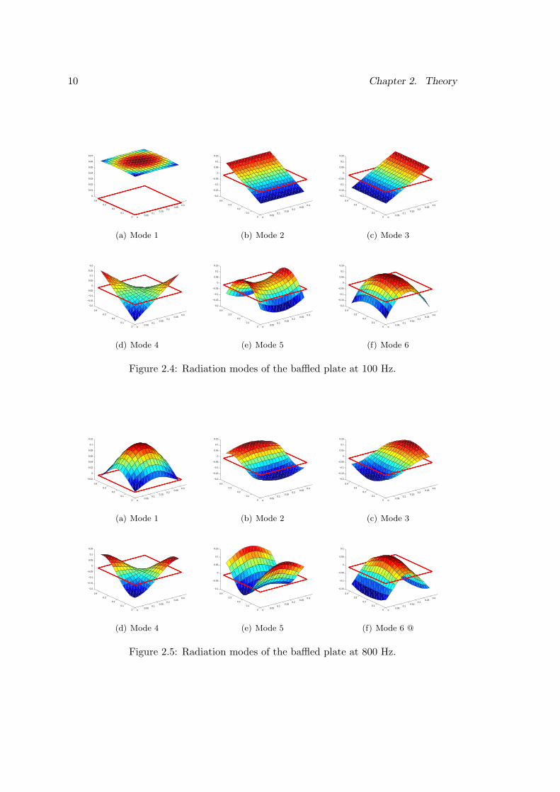
2.5 Radiation Modes

The eigenvalues of the radiation resistance matrix R are proportional to the radiationefficiencies and the eigencolumns are known as the radiation modes. These radiationmodes are frequency dependent and indicate the contribution of each element to thetotal radiated sound power. For the aluminium plate with the properties listed in Table2.1 the shapes of the first six radiation modes and their corresponding eigenvalue λr,which are proportional to the radiation efficiencies, have been calculated, see Figures2.3, 2.4 and 2.5. The eigenvalues λr are linear increasing with the frequency at lowfrequencies. For frequencies under 1 kHz the first radiation mode is by far the mostefficient one. Above 1 kHz the different modes are equally efficient. The radiationmodes are frequency dependent and are plotted at two frequencies, f1 = 100 Hz andf2 = 800 Hz. Figures 2.4 and 2.5 clearly shows that the first, and most efficient mode,

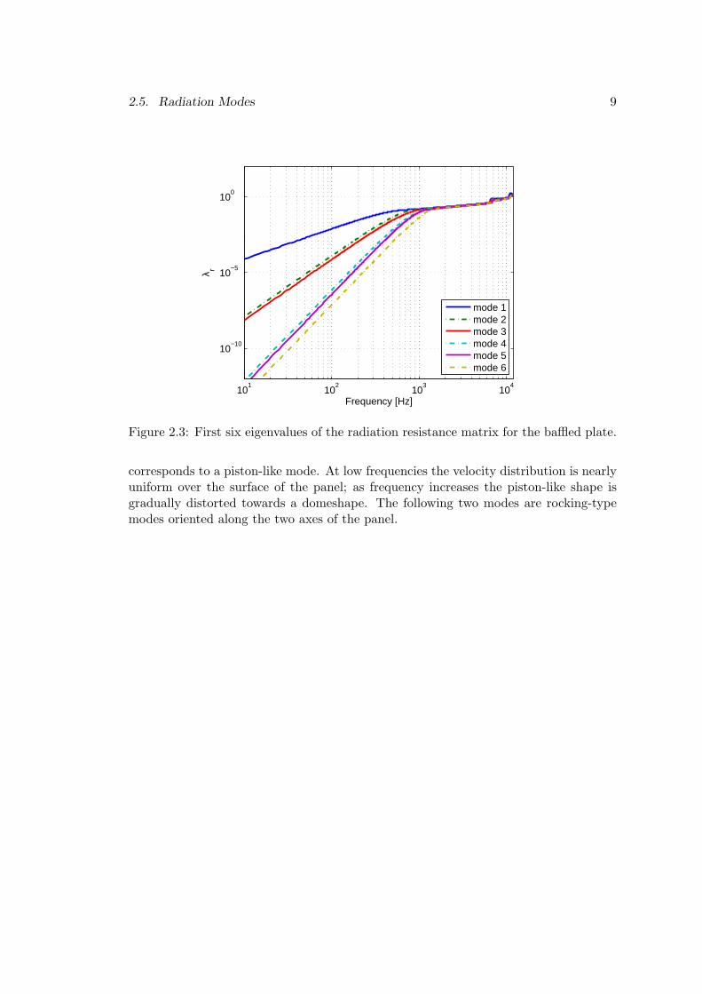
2.5. Radiation Modes 9

101

102

103

104

10−10

10−5

100

Frequency [Hz]

λ r

mode 1mode 2mode 3mode 4mode 5mode 6

Figure 2.3: First six eigenvalues of the radiation resistance matrix for the baffled plate.

corresponds to a piston-like mode. At low frequencies the velocity distribution is nearlyuniform over the surface of the panel; as frequency increases the piston-like shape isgradually distorted towards a domeshape. The following two modes are rocking-typemodes oriented along the two axes of the panel.

10 Chapter 2. Theory

00.05

0.10.15

0.20.25

0.3

0

0.1

0.2

0.3

0.4

0

0.01

0.02

0.03

0.04

0.05

0.06

0.07

(a) Mode 1

00.05

0.10.15

0.20.25

0.3

0

0.1

0.2

0.3

0.4

−0.2

−0.15

−0.1

−0.05

0

0.05

0.1

0.15

(b) Mode 2

00.05

0.10.15

0.20.25

0.3

0

0.1

0.2

0.3

0.4

−0.2

−0.15

−0.1

−0.05

0

0.05

0.1

0.15

(c) Mode 3

00.05

0.10.15

0.20.25

0.3

0

0.1

0.2

0.3

0.4

−0.2

−0.15

−0.1

−0.05

0

0.05

0.1

0.15

0.2

(d) Mode 4

00.05

0.10.15

0.20.25

0.3

0

0.1

0.2

0.3

0.4

−0.2

−0.15

−0.1

−0.05

0

0.05

0.1

0.15

(e) Mode 5

00.05

0.10.15

0.20.25

0.3

0

0.1

0.2

0.3

0.4

−0.2

−0.15

−0.1

−0.05

0

0.05

0.1

0.15

(f) Mode 6

Figure 2.4: Radiation modes of the baffled plate at 100 Hz.

00.05

0.10.15

0.20.25

0.3

0

0.1

0.2

0.3

0.4

−0.02

0

0.02

0.04

0.06

0.08

0.1

0.12

(a) Mode 1

00.05

0.10.15

0.20.25

0.3

0

0.1

0.2

0.3

0.4

−0.2

−0.15

−0.1

−0.05

0

0.05

0.1

0.15

(b) Mode 2

00.05

0.10.15

0.20.25

0.3

0

0.1

0.2

0.3

0.4

−0.2

−0.15

−0.1

−0.05

0

0.05

0.1

0.15

(c) Mode 3

00.05

0.10.15

0.20.25

0.3

0

0.1

0.2

0.3

0.4

−0.2

−0.15

−0.1

−0.05

0

0.05

0.1

0.15

(d) Mode 4

00.05

0.10.15

0.20.25

0.3

0

0.1

0.2

0.3

0.4

−0.1

−0.05

0

0.05

0.1

0.15

(e) Mode 5

00.05

0.10.15

0.20.25

0.3

0

0.1

0.2

0.3

0.4

−0.15

−0.1

−0.05

0

0.05

0.1

(f) Mode 6 @


Chapter 3

Numerical results

In literature [Fah87] the eigenfrequencies and radiation efficiencies for a finite baffledplate can be found and are mentioned in Chapter 2. By discretizing the plate intofinite elements numerical methods in software packages can be used to calculate theeigenfrequencies and radiation efficiencies and they are compared with the theoreticalvalues.

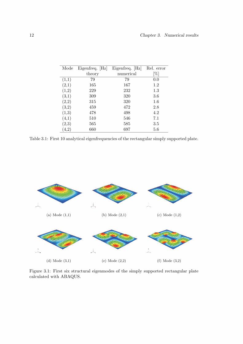
3.1 Eigenfrequencies and mode shapes

In Chapter 2 the theory about the eigenfrequencies of a simply supported finite plateis presented. In ABAQUS this simply supported plate is modeled with 16 by 16 shellelements. In Appendix A the input file that is used in ABAQUS can be found. InFigure 3.1 the mode shapes calculated with ABAQUS can be found and in Table 3.1the theoretical and numerical (ABAQUS) eigenfrequencies are denoted. As can be seenthe relative error between the eigenfrequencies is bigger for higher frequencies. Thenumerical eigenfrequencies are higher than the theoretical eigenfrequencies, because thediscretized model has a certain number of degrees of freedom (dof’s). When more ele-ments would be used this number of dof’s will increase, which results in a less stiff plateand consequently lower eigenfrequencies. Also the number of elements per structuralwavelength should be examined; at least six elements per wavelength should be used.

3.2 Radiation efficiencies and modes

As described in Chapter 2.5 the radiation efficiency is proportional to the eigenvaluesof the radiation resistance matrix R = S

2RRe(B). To compare the eigenvalues of theradiation resistance matrix obtained from an BE analysis the (complex) influence matrixB is exported from LMS Virtual.Lab. This is done for 10 different frequencies at

11

12 Chapter 3. Numerical results

Mode Eigenfreq. [Hz] Eigenfreq. [Hz] Rel. errortheory numerical [%]

(1,1) 79 79 0.0(2,1) 165 167 1.2(1,2) 229 232 1.3(3,1) 309 320 3.6(2,2) 315 320 1.6(3,2) 459 472 2.8(1,3) 478 498 4.2(4,1) 510 546 7.1(2,3) 565 585 3.5(4,2) 660 697 5.6

Table 3.1: First 10 analytical eigenfrequencies of the rectangular simply supported plate.

(a) Mode (1,1) (b) Mode (2,1) (c) Mode (1,2)

(d) Mode (3,1) (e) Mode (2,2) (f) Mode (3,2)

Figure 3.1: First six structural eigenmodes of the simply supported rectangular platecalculated with ABAQUS.

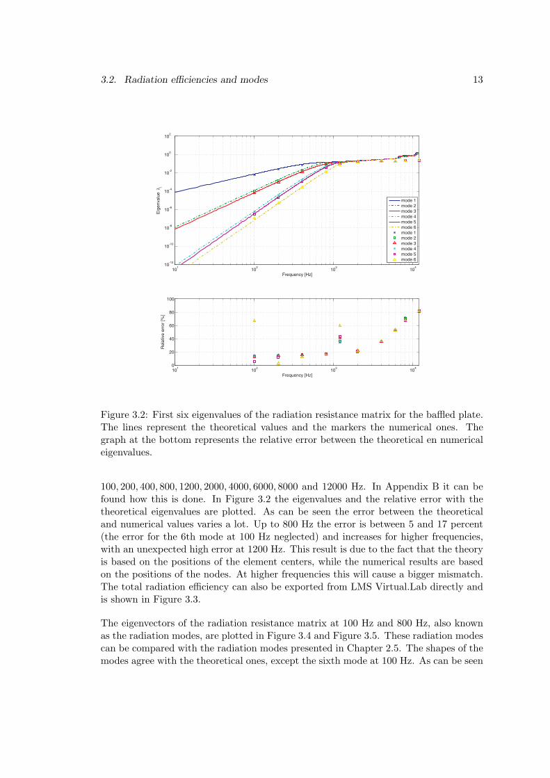
3.2. Radiation efficiencies and modes 13

Figure 3.2: First six eigenvalues of the radiation resistance matrix for the baffled plate.The lines represent the theoretical values and the markers the numerical ones. Thegraph at the bottom represents the relative error between the theoretical en numericaleigenvalues.

100, 200, 400, 800, 1200, 2000, 4000, 6000, 8000 and 12000 Hz. In Appendix B it can befound how this is done. In Figure 3.2 the eigenvalues and the relative error with thetheoretical eigenvalues are plotted. As can be seen the error between the theoreticaland numerical values varies a lot. Up to 800 Hz the error is between 5 and 17 percent(the error for the 6th mode at 100 Hz neglected) and increases for higher frequencies,with an unexpected high error at 1200 Hz. This result is due to the fact that the theoryis based on the positions of the element centers, while the numerical results are basedon the positions of the nodes. At higher frequencies this will cause a bigger mismatch.The total radiation efficiency can also be exported from LMS Virtual.Lab directly andis shown in Figure 3.3.

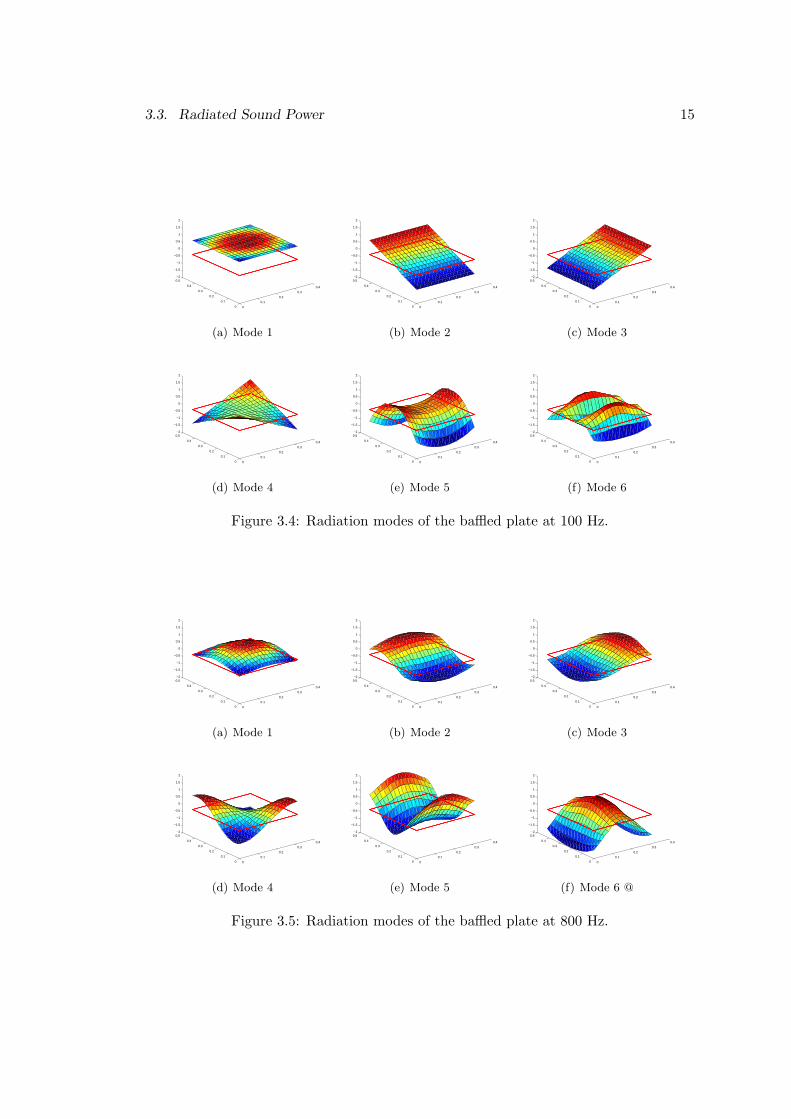
The eigenvectors of the radiation resistance matrix at 100 Hz and 800 Hz, also knownas the radiation modes, are plotted in Figure 3.4 and Figure 3.5. These radiation modescan be compared with the radiation modes presented in Chapter 2.5. The shapes of themodes agree with the theoretical ones, except the sixth mode at 100 Hz. As can be seen


101

102

103

104

10−4

10−3

10−2

10−1

100

101

Frequency [Hz]

Rad

iatio

n ef

ficie

ncy

Figure 3.3: Radiation efficiency exported from LMS Virtual.Lab.

in Figure 3.2 the eigenvalue for this mode does not agree with the theoretical value aswell. Within this report there is not an explanation for this result.

3.3 Radiated Sound Power

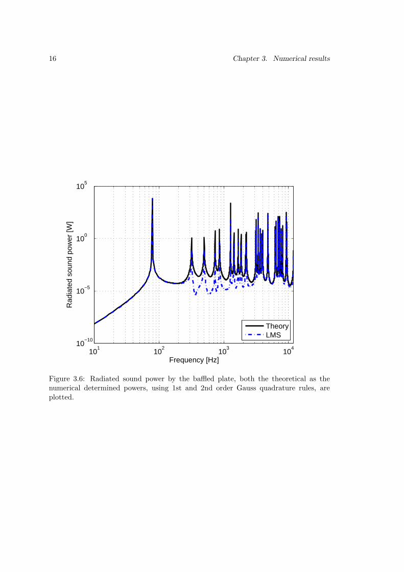
The total sound power radiated by the baffled plate for a given velocity distributioncan be calculated using (2.13). A harmonic point force with an amplitude of 1 N at thecenter and perpendicular to the plate is used to calculate the velocity distribution atthe nodes of the plate within ABAQUS. A frequency range of 1 Hz to 12001 Hz witha linear step-size of 2 Hz is used. This velocity distribution is interpolated bi-linearlyto the element centers, because the theoretical radiation resistance matrix R is definedusing the element centers and is given as in (2.15). From simulations with the BEsoftware package LMS Virtual.Lab the radiated sound power can be exported. Thesesimulations use Gaussian quadrature rules for the numerical integration of the Helmholtzintegral equation. In LMS Virtual.Lab the quadrature, i.e. the number of Gauss pointsused in one direction for the numerical evaluation of integrals, are by default set to thevalues of 2, 2, 1 for the different regions (near, medium and far respectively). In thisreport only the near field region is examined. In Figure 3.6 the results for the totalradiated sound power using both the theory and the numerical results are shown.

As can be seen in Figure 3.6 the radiated power is characterised by a sequence of

3.3. Radiated Sound Power 15

0

0.1

0.2

0.3

0.4

0

0.1

0.2

0.3

0.4

0.5−2

−1.5

−1

−0.5

0

0.5

1

1.5

2

(a) Mode 1

0

0.1

0.2

0.3

0.4

0

0.1

0.2

0.3

0.4

0.5−2

−1.5

−1

−0.5

0

0.5

1

1.5

2

(b) Mode 2

0

0.1

0.2

0.3

0.4

0

0.1

0.2

0.3

0.4

0.5−2

−1.5

−1

−0.5

0

0.5

1

1.5

2

(c) Mode 3

0

0.1

0.2

0.3

0.4

0

0.1

0.2

0.3

0.4

0.5−2

−1.5

−1

−0.5

0

0.5

1

1.5

2

(d) Mode 4

0

0.1

0.2

0.3

0.4

0

0.1

0.2

0.3

0.4

0.5−2

−1.5

−1

−0.5

0

0.5

1

1.5

2

(e) Mode 5

0

0.1

0.2

0.3

0.4

0

0.1

0.2

0.3

0.4

0.5−2

−1.5

−1

−0.5

0

0.5

1

1.5

2

(f) Mode 6


0

0.1

0.2

0.3

0.4

0

0.1

0.2

0.3

0.4

0.5−2

−1.5

−1

−0.5

0

0.5

1

1.5

2

(a) Mode 1

0

0.1

0.2

0.3

0.4

0

0.1

0.2

0.3

0.4

0.5−2

−1.5

−1

−0.5

0

0.5

1

1.5

2

(b) Mode 2

0

0.1

0.2

0.3

0.4

0

0.1

0.2

0.3

0.4

0.5−2

−1.5

−1

−0.5

0

0.5

1

1.5

2

(c) Mode 3

0

0.1

0.2

0.3

0.4

0

0.1

0.2

0.3

0.4

0.5−2

−1.5

−1

−0.5

0

0.5

1

1.5

2

(d) Mode 4

0

0.1

0.2

0.3

0.4

0

0.1

0.2

0.3

0.4

0.5−2

−1.5

−1

−0.5

0

0.5

1

1.5

2

(e) Mode 5

0

0.1

0.2

0.3

0.4

0

0.1

0.2

0.3

0.4

0.5−2

−1.5

−1

−0.5

0

0.5

1

1.5

2

(f) Mode 6 @



101

102

103

104

10−10

10−5

100

105

Frequency [Hz]

Rad

iate

d so

und

pow

er [W

]

TheoryLMS

Figure 3.6: Radiated sound power by the baffled plate, both the theoretical as thenumerical determined powers, using 1st and 2nd order Gauss quadrature rules, areplotted.

3.3. Radiated Sound Power 17

peaks corresponding to the eigenfrequencies of the plate. Note that the peaks do notcorrespond with all structural eigenfrequencies. The first four peaks correspond withthe (1,1), (3,1), (1,3) and (3,3) mode respectively. These odd-odd modes are symmetricmodes and radiate sound efficiently. The even (asymmetric) modes do not radiate soundefficiently. For example, the (2,1) mode shape is an asymmetric mode, that causes ahigh pressure at one half of the plate and a low pressure at the other half at the sametime. In this way the variation in pressure at the surface caused by the two parts of theplate cancel each contribution to the total radiated power.

Between 200 and 3000 Hz a large mismatch between the theoretical and numerical soundpower can be seen. This is due to the different methods of interpolation that are used.In theory the element centers are used. Therefore the velocities at the nodes are bi-linearly interpolated to the element center. This means that the four surrounded nodeseach have the same contribution to the resulting value at the center of the element. InGaussian quadrature, both the nodes and the weights are optimally chosen to maximizethe degree of the resulting quadrature rule [Hea02]. In LMS Virtual.Lab two Gausspoint are used, resulting in quadrature rules of degree three. Gaussian quadraturerules therefore have a higher accuracy than the bi-linearly interpolation used for thetheoretical results.


Chapter 4

Implementation

In this Chapter the implementation of a model of the baffled plate in the various softwareprograms is described in more detail. Moreover, the various steps of modeling, exportingand importing the results is described in a chronological way.

4.1 ABAQUS

First to obtain the vibrational data that causes the radiated sound, a simply supportedrectangular aluminium plate is modeled within ABAQUS. An input file with extension.inp is written, see Appendix A. In this input file first a grid of 17 by 17 nodes isdefined. Next step is defining the 16 by 16 quadrilateral shell elements, with a virtual3th dimension with a size of 2 mm (the thickness of the plate). The edges of the plateare simply supported, so a boundary condition is defined to set all translational (so notrotational) degrees of freedom at the corresponding nodes to zero. Finally two steps areapplied, the first to calculate the first 10 eigenfrequencies and the second to calculatethe velocities at the nodes generated by a harmonic point force at the center of the platefor different frequencies.

This input file can be run in the ABAQUS command window by typing

abaqus job = filename .

Now ABAQUS will generate an database file with extension .odb containing the results.Also an .dat file will be created, which may be handy for debugging the input file. The.odb file can be opened in the ABAQUS Viewer to see the results. Moreover, thecalculated velocity distribution can be exported to a text file (.txt), which can beimported in Matlab.

19

20 Chapter 4. Implementation

Figure 4.1: Select the Mesh Coarsening workbench.

4.2 LMS Virtual.Lab

A very common application of LMS Virtual.Lab is to compute the sound field radiatedby a vibrating structure. To characterize the structural vibrations in LMS Virtual.Laba structural finite element analysis, like the .odb file from ABAQUS, can be imported.In this way the mesh and analysis steps from ABAQUS can be used in LMS.

4.2.1 Mesh Coarsening

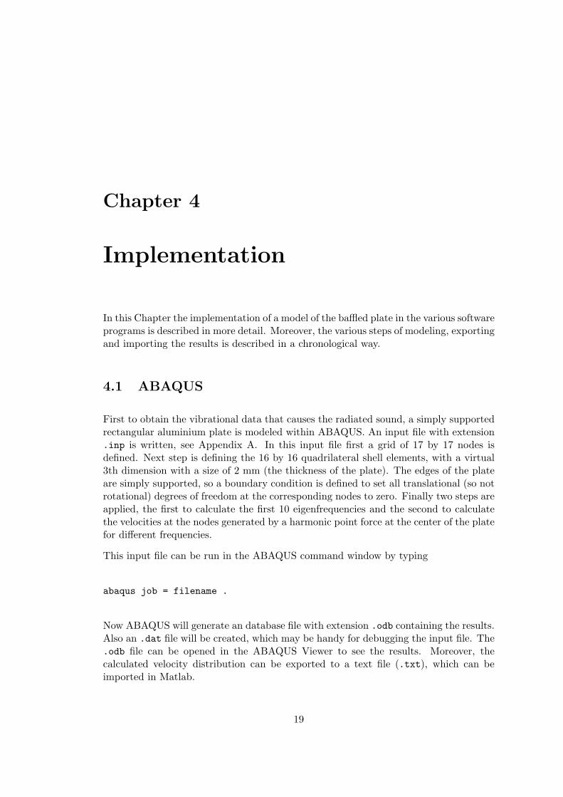
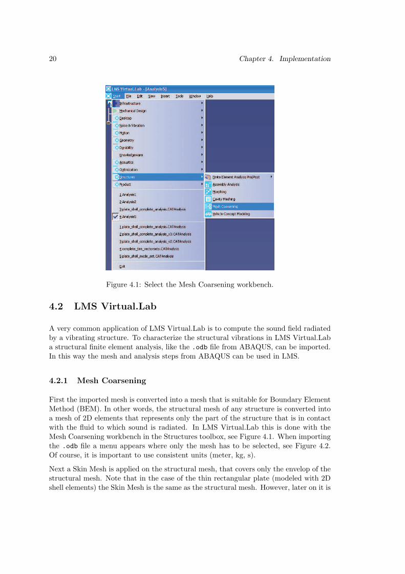
First the imported mesh is converted into a mesh that is suitable for Boundary ElementMethod (BEM). In other words, the structural mesh of any structure is converted intoa mesh of 2D elements that represents only the part of the structure that is in contactwith the fluid to which sound is radiated. In LMS Virtual.Lab this is done with theMesh Coarsening workbench in the Structures toolbox, see Figure 4.1. When importingthe .odb file a menu appears where only the mesh has to be selected, see Figure 4.2.Of course, it is important to use consistent units (meter, kg, s).

Next a Skin Mesh is applied on the structural mesh, that covers only the envelop of thestructural mesh. Note that in the case of the thin rectangular plate (modeled with 2Dshell elements) the Skin Mesh is the same as the structural mesh. However, later on it is

4.2. LMS Virtual.Lab 21

Figure 4.2: Import the structural mesh.


Figure 4.3: Export the Skin Mesh.

needed to have both a Skin (acoustic) Mesh to apply the acoustic boundary conditionsto and a structural mesh with the vibrational data. For more complex structures it canbe desired to fill holes, convert element types or delete unwanted elements to create anoptimal acoustic mesh. This is also possible in the Structures toolbox.

Finally the Skin Mesh part has to be exported to an external file, e.g. a Nastran bulkfile (.bdf), see Figure 4.3.

4.2.2 Load Vector Set

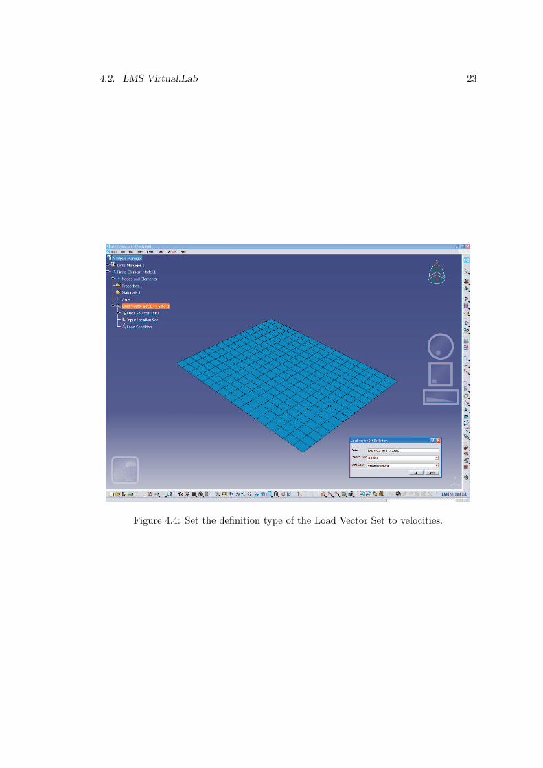
The structural vibrational data from ABAQUS is imported as a Load Vector Set intoLMS Virtual.Lab. A new System Analysis with the Noise and Vibrations toolbox isstarted and the .odb file is imported. This time the mesh and Step 2 from the LoadVector Sets are toggled on. This will create a Load Vector Set in the specificationtree. The definition type of this Load Vector Set is set to velocities, as it contains thevelocities calculated with ABAQUS, by double clicking on the Load Vector Set, seeFigure 4.4. By generating an image of the Set, the velocities can be visualized in LMSVirtual.Lab. Finally this analysis is saved as a CATAnalysis document.


Figure 4.4: Set the definition type of the Load Vector Set to velocities.


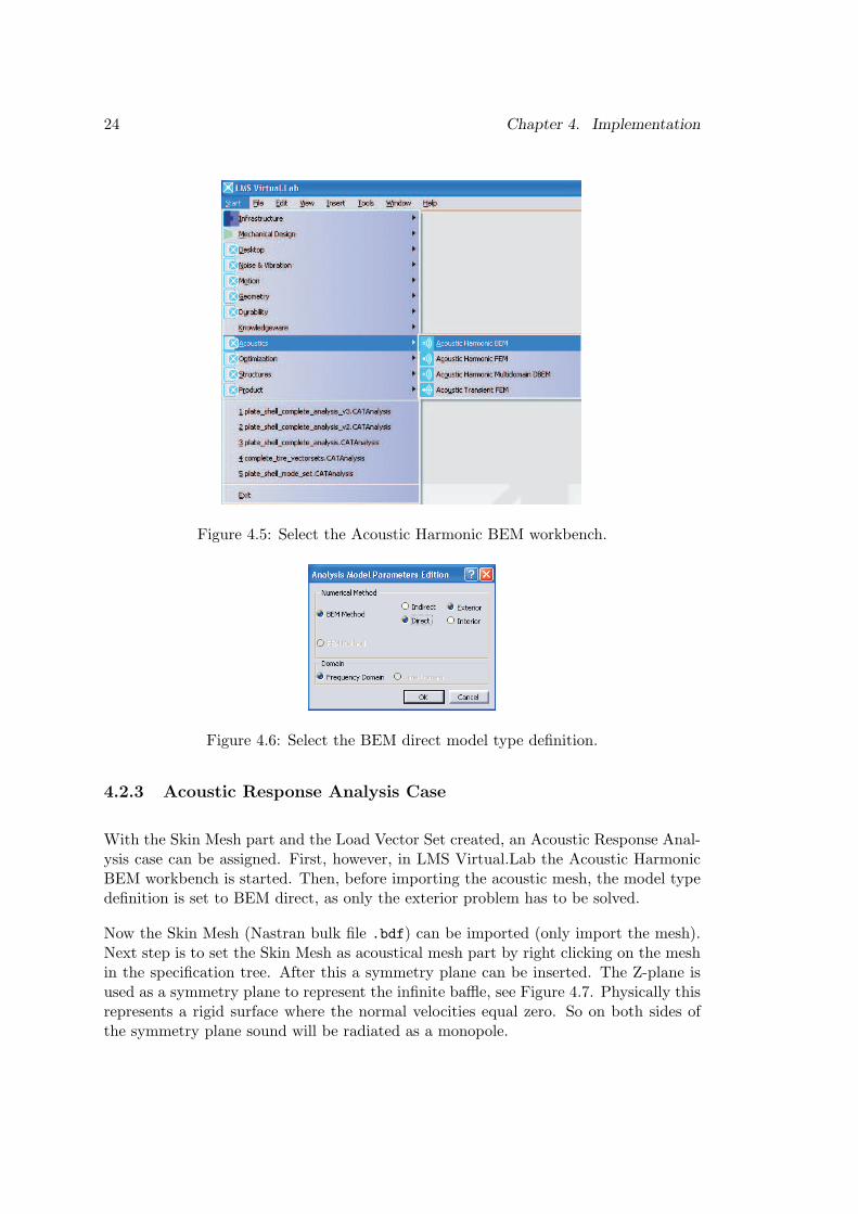
Figure 4.5: Select the Acoustic Harmonic BEM workbench.

Figure 4.6: Select the BEM direct model type definition.

4.2.3 Acoustic Response Analysis Case

With the Skin Mesh part and the Load Vector Set created, an Acoustic Response Anal-ysis case can be assigned. First, however, in LMS Virtual.Lab the Acoustic HarmonicBEM workbench is started. Then, before importing the acoustic mesh, the model typedefinition is set to BEM direct, as only the exterior problem has to be solved.

Now the Skin Mesh (Nastran bulk file .bdf) can be imported (only import the mesh).Next step is to set the Skin Mesh as acoustical mesh part by right clicking on the meshin the specification tree. After this a symmetry plane can be inserted. The Z-plane isused as a symmetry plane to represent the infinite baffle, see Figure 4.7. Physically thisrepresents a rigid surface where the normal velocities equal zero. So on both sides ofthe symmetry plane sound will be radiated as a monopole.


Figure 4.7: The symmetry plane that represents the infinite baffle.


Figure 4.8: The Data Transfer Analysis case.

The BEM direct methodology requires a strictly consistent mesh definition. The di-rection of the element normal vectors have to be consistent and on free edges the freeedge boundary condition should be applied. This is achieved by the Mesh Preprocess-ing Set. LMS Virtual.Lab will automatically prepare the acoustic mesh such that itcomplies with these requirements. This is achieved by inserting a Mesh PreprocessingSet, selecting the acoustic mesh and clicking update.

Next step is to apply a new fluid material and property. In this case the fluid mediumis air and it can be inserted from the insert menu.

The following step is to insert a Data Transfer Analysis case to transfer the vibrationaldata from the Load Vector Set to the acoustic mesh. First the structural CATAnalysisfile that contains the Load Vector Set is imported into the recent analysis. Next theData Transfer Analysis Case is created. In the Data Transfer Analysis Case dialog,Create a New Mesh Mapping Set is selected and the Load Vector Set is selected totransfer. This will create a new Data Transfer Analysis Case in the specification tree.Now the acoustic mesh is set as the Target Set and the structural mesh (in the linksmanager) as the Source Set. In the Mapping Data feature the MaxDistance algorithmis used to transfer the structural vibrations data to the acoustic mesh. In Figure 4.8 itcan be seen what the specification tree looks like at this moment.


Figure 4.9: The specification tree after inserting the Boundary Condition Set.

To define vibration boundary conditions a Boundary Condition Set feature is insertedin the specification tree. The Load Conditions are set to Automatic and the loadconditions to DataSource + Test/Subcase. Then a Boundary Condition, with velocitiesas physical type and vector as mathematical type, are added. The acoustic mesh part isassigned under the Faces feature and the Data Transfer Set is assigned under the DataSource feature. This completes the Boundary Condition Set and the specification treebecomes like in Figure 4.9.

Finally the Acoustic Response Analysis Case is created. In the Acoustic ResponseAnalysis Case dialog the just created Boundary Condition Set can be assigned. Thesolution parameters of the Acoustic Response Analysis Case can be adjusted, e.g. forthe frequency spectra the values from the boundary conditions can be used. Also itcan be adjusted whether SYSNOISE performs the computations in synchronous mode(LMS waits for SYSNOISE to complete the job, while it is possible to use other softwaresimultaneously) or in manual mode (LMS creates files to be executed by SYSNOISEseparately, outside LMS). The latter one will use all computer power available andconsequently will be faster. Moreover, some adjustments can be made to these files forextra options, like exporting the BEM matrices A and B. This is discussed in moredetail in Appendix B.


Chapter 5

Conclusion andRecommendations

In this report numerical results for the sound radiation of a baffled rectangular plateis compared with theory. For the structural vibration analysis ABAQUS is used todetermine the response of the plate to a harmonic point force. Moreover, ABAQUSis used to calculate the first ten eigenfrequencies of the plate. These eigenfrequenciesmatch the theoretical eigenfrequencies up to 92.9 %. To get a better match between thenumerical and theoretical eigenfrequencies, especially for the higher frequencies, moreelements should be used.

For the acoustic response analysis LMS Virtual.Lab and SYSNOISE are used. Thetheoretical and numerical eigenvalues of the radiation resistance matrix are compared.They match up to 83 % for frequencies below 1200 Hz. Above this frequency the errorwill grow. The numerical results for the total radiated sound power agrees well withthe theory for low frequencies, below 240 Hz. Above this frequency the results matchless. This is due to the different interpolation functions that are used. The theoreticalresults are obtained by a bilinear interpolation of the velocities at the nodes to theelement centers, while the numerical integration uses Gauss quadrature rules using twoGauss points, which will give more accurate results. Besides the use of more accuratequadrature rules, more elements will give better results in the acoustic analysis forhigher frequencies, so that more elements per wavelength are used.

29

30 Chapter 5. Conclusion and Recommendations

Bibliography

[Fah87] F. Fahy and P. Gardonio. Sound and structural vibration, radiation, transmis-sion and response. 2:145–175, 1987.

[Hea02] M.T. Heath. Scientific computing, an introductory survey. 2:351–353, 2002.

[Vis04] R. Vissers. A boundary element approach to acoustic radiation and sourceidentification. 1:22–52, 2004.

31

32 Bibliography

Appendix A

ABAQUS input file

The input file for ABAQUS that is used for the numerical results in the structuralanalysis of the plate is listed below.

*HEADING

PLATE

*NODE, NSET=ENDS

1, 0., 0., 0.

17, 0.314, 0., 0.

273, 0., 0.414, 0.

289, 0.314, 0.414,0.

*NGEN

1, 17, 1

1, 273, 17

17, 289, 17

273, 289, 1

18, 34, 1

35, 51, 1

52, 68, 1

69, 85, 1

86, 102, 1

103, 119, 1

120, 136, 1

137, 153, 1

154, 170, 1

171, 187, 1

188, 204, 1

205, 221, 1

222, 238, 1

239, 255, 1

256, 272, 1

273, 289, 1

*NSET,NSET=RAND,GENERATE,UNSORTED

1, 17, 1

18, 256, 17

273, 289, 1

34, 272, 17

*NSET,NSET=BASE,GENERATE,UNSORTED

1, 289, 1

*ELEMENT, TYPE=S4

33

34 Appendix A. ABAQUS input file

1, 1, 2, 19, 18

*ELGEN

1, 16, 1, 1, 16, 17, 16

*ELSET, ELSET=PLATE, GENERATE

1, 256, 1

*SHELL SECTION, ELSET=PLATE, MATERIAL=ALU

0.002

*MATERIAL, NAME=ALU

*ELASTIC

71.E9, 0.33

*DENSITY

2700

*BOUNDARY

RAND, 1,3

********************************************

********************************************

*STEP,INC=1,NLGEOM=YES

1: FREQUENCY_ANALYSIS

*FREQUENCY, EIGENSOLVER=LANCZOS

10

*BOUNDARY,OP=NEW

RAND, 1,3

*EL PRINT,FREQ=0

*OUTPUT,FIELD,FREQ=1

*NODE OUTPUT

U

*OUTPUT,HISTORY,FREQ=1

*END STEP

*********************************************

*********************************************

*STEP,NLGEOM=YES

2: FREQUENCY RESPONSE: STEADY STATE DYNAMICS,

DIRECT

*STEADY STATE DYNAMICS,DIRECT,

INTERVAL=RANGE,FREQUENCY SCALE=LINEAR

1,12001,6000

*CLOAD

145,3,1.

*OUTPUT,FIELD,FREQ=1

*NODE OUTPUT

V

*OUTPUT,HISTORY,FREQ=1

*END STEP

Appendix B

Export of BEM matrices

The acoustic response calculations are executed with LMS Virtual.Lab and SYSNOISE.The calculated A and B matrices in (2.5) can be exported to a file in a so called freeformat. This is only possible to calculate for a direct BEM uncoupled analysis. Tocalculate the matrices the Acoustic Response Analysis Case has to be executed manuallyresulting in a new .cmd and .bat file in the specified folder. Now the .cmd file has tobe adapted with the following command:

COMPUTE ABMATRIX

FILE "filename" FORMAT Free

FREQUENCY "beginfrequency" TO "endfrequency" LINSTEP "frequencystep"

NEAR 2

FAR 5

QUADRATURE 2 2 1

RETURN

Next step is to execute the .bat file by double clicking this file. It will use SYSNOISEwith no graphical user interface installed in the LMS Virtual.Lab destination folderto create a sysnoise database file with extension .sdb, that has to be attached to theAcoustic Response Analysis Case in LMS Virtual.Lab.

The used .cmd file for the numerical results from this report is listed below:

ENVIRONMENT SECTION SETUP USRDIR ’D:\Arjan\Sysnoise\’ RETURN

ENVIRONMENT SECTION SETUP TMPDIR ’D:\Arjan\Sysnoise\’ RETURN

Open Model 1 File s030293-638-Acoustic.sdb Original Return

Extract Summary Return

Environment Section SETUP BELL ’on’ Return

Environment Section SETUP GEO_TOLERANCE ’0.001’ Return

Parameter Model 1

Physical

Save Potentials Step 1

Save Results none

Store Results none

Return

35

36 Appendix B. Export of BEM matrices

Near 2

Far 5

Quadrature 2 2 1

Return

Solve

Frequency 0 1 3 5 7 9

...

Frequency 11989 11991 11993 11995 11997 11999

Frequency 12001

Return

Save Return

COMPUTE ABMATRIX

FILE bemmatrices FORMAT Free

FREQUENCY 2000 TO 8000 LINSTEP 2000

NEAR 2

FAR 5

QUADRATURE 2 2 1

RETURN

Close Return

New Model 1 File s030293-638-SignalFile.sdb Return

Save Return

Exit

This script will create the files bemmatrices.fre and s030293-638-SignalFile.sdbcontaining the BEM matrices and the results of the Acoustic Response Analysis Caserespectively.

The bemmatrices.fre file has the following layout:

Header Section

TITLE Title

NNBEM Number of BEM nodes (number of elements in contact with the air)

LNUSR List of BEM nodes (external numbers)

Matrix Section

Freq Frequency

AMATR [A] matrix written column by column

BMATR [B] matrix written column by column

The header section is written only once. The matrix section can be written severaltimes, once for each frequency. On each line three complex coefficients are written. So,in the case of the plate with 289 nodes, each matrix is represented by 83521 (289 times289) complex numbers. Consequently, the bemmatrices.fre file will contain 167042 (2times 83521) complex coefficients for each the A and B matrix.

To import the results in Matlab, first for each frequency a new text file with only thecontents of the matrices is distracted from the bemmatrices.fre file. Secondly, a newcomplex matrix can be distracted from this text file.

Documents

Sound radiation of a ba†ed plate; theoretical and ... · PDF file2.2 Boundary Element Method ... together with SYSNOISE for ... total radiated sound power normalized with respect