Embed Size (px)
Citation preview
Sound Quality User-defined Cursor Reading Control
-Tonality Metric
Zhong Zhang (s001071) Merina Shrestha (s001078)
IMM, DTU Brüel & Kjær
10/03/2003

Sound Quality User-defined Cursor Reading Control - Tonality Metric
Abstract Sound Quality as a relatively new product parameter has become an important competition item among the car manufactures. Sound Quality metrics is the same as Sound Quality parameters, which can reflect most of the psychoacoustic properties of the human perception of sound. There are some standardized metrics, such as Stationary Loudness, Tone to Noise Ratio, Prominence ratio, but most metrics are not standardized. They all have the advantage that they conclude with a single number on the characteristic properties of the sound. Tonality is one of the Sound Quality metrics that is not yet standardized, but it is an important parameter affecting Sound Quality because it is proportional to the human perception of tonal contents in the sound. Terhardt’s Tonality, which was proposed in 1892, is an algorithm for extraction of pitch and pitch salience from complex tonal signals. It is widely accepted that Terhardt’s method is the foundation for Tonality metric definition. Studying Terhardt’s algorithm is the start point of this thesis project. A MATLAB model according to Terhardt’s algorithm is made. AVC++ implementation is also made in order to make it ready for Brüel & Kjær Sound Quality Application to use. Furthermore, both MATLAB and VC++ programs have been tested, and validated for further research work. An overall study of Stationary Loudness and Aures’s Model of Tonality is also provided by our thesis. They broaden our knowledge in psychoacoustics research field.
1
Sound Quality User-defined Cursor Reading Control - Tonality Metric
Preface This master thesis has been carried out under the cooperation between Informatics and Mathematical Modelling Department (IMM), Technical University of Denmark (DTU), and Brüel & Kjær Sound and Vibration A/S, from Sep 9, 2002 to Mar 10, 2003. March 10, 2003 Zhong Zhang s001071 Merina Shrestha s001078
2
Sound Quality User-defined Cursor Reading Control - Tonality Metric
Acknowledgements We would like to express our sincere thanks to our thesis supervisors, Jens Thyge Kristensen and Henrik Haslev, who are on behalf of IMM, DTU and B&K respectively, for their nice guidance and suggestions during our thesis period. We would like to thank Svend Lysemose, Poul Ladegaard, Tommy Schack, Howard Mealor, Jacob Juhl Christensen and all colleagues in Sound Quality group in B&K for providing us such a convenient and friendly work environment. We would like to thank Torben Poulsen, Aaron Hastings, Wolfgang Ellermeier for providing us the helpful information.
3

Sound Quality User-defined Cursor Reading Control - Tonality Metric
Abbreviations ANSI American National Standards Institute B&K Brüel & Kjær CPB Constant Percentage Bands DFD Data Flow Diagram DIN German Standard FFT Fast Fourier Transform ISO The International Organization for Standardization SPL Sound Pressure Level SQ Sound Quality
4
Sound Quality User-defined Cursor Reading Control - Tonality Metric
Contents
Chapter 1 Introduction_______________________________________________ 10
1.1 Problem definition__________________________________________ 10
1.2 Our Difficulties and Strategies________________________________ 10
1.3 Working Process ___________________________________________ 13
1.4 Thesis Organization ________________________________________ 14
Chapter 2 Specific Background Knowledge for this Thesis __________________ 15
2.1 Sound Quality ________________________________________________ 16 2.1.1 What is Sound Quality? ______________________________________ 16 2.1.2 Why improve the Quality of Sound? ____________________________ 16 2.1.3 Work with Sound Quality ____________________________________ 16 2.1.4 Optimisation of Sound Quality Analysis _________________________ 18
2.2 Psychoacoustics _______________________________________________ 18 2.2.1 Stimuli and Sensations _______________________________________ 19 2.2.2 Hearing Area ______________________________________________ 19 2.2.3 Equal Loudness Contours and A-weighting_______________________ 20 2.2.4 Masking __________________________________________________ 21 2.2.5 Critical Bands______________________________________________ 24 2.2.6 Bark Scale ________________________________________________ 25 2.2.7 Model of Virtual Pitch _______________________________________ 26
2.3 Sound Quality Metrics _________________________________________ 29
2.4 Tonality Metric _______________________________________________ 30
2.5 Terms and Definitions__________________________________________ 30
Chapter 3 Review Tonality Algorithm ___________________________________ 37
3.1 Spectrum Analysis_____________________________________________ 38
3.2 Extraction of Tonal Components_________________________________ 38
3.3 Evaluation of Masking Effects ___________________________________ 39 3.3.1 Sound-pressure Level Excess__________________________________ 39 3.3.2 Pitch Shifts ________________________________________________ 40
3.4 Weighting of Components ______________________________________ 42
3.5 Evaluation of Virtual Pitch______________________________________ 42
Chapter 4 Tonality Model in MATLAB__________________________________ 45
4.1 What is MATLAB? ____________________________________________ 45
4.2 What is M-file ________________________________________________ 45
4.3 Data Flow of Tonality Model ____________________________________ 46
4.4 Model Simplification and Modification____________________________ 49
4.5 The Relations of Different M-files in Tonality MATLAB Model _______ 50
4.6 A Function M-file Example _____________________________________ 51
5
Sound Quality User-defined Cursor Reading Control - Tonality Metric
4.7 How to Show the Computational Results? _________________________ 53
4.8 Model Testing ________________________________________________ 55
Chapter 5 Implementation of Tonality Metric for SQ Application in VC++_____ 57
5.1 How COM Component being used in our Project? _______________ 57 5.1.1 What is a Template Library? __________________________________ 57 5.1.2 More about COM Programming _______________________________ 57 5.1.3 What is Dynamic Link Libraries (DLL)?_________________________ 58 5.1.4 Using COM in SQ Application ________________________________ 58 5.1.5 More about COM Interface ___________________________________ 61
5.2 Tonality Implementation in VC++ ____________________________ 62 5.2.1 Why Choose Vector Container Type? _______________________ 63 5.2.2 Using Pointers __________________________________________ 64 5.2.3 Using The Generic Algorithms _____________________________ 66 5.2.4 Object-based Programming________________________________ 67
Chapter 6 Testing of MATLAB and VC++ Program _______________________ 70
Chapter 7 Further Study _____________________________________________ 75
7.1 Loudness_____________________________________________________ 75 7.1.1 Stationary Loudness and Non-stationary Loudness_________________ 75 7.1.2 Method A and Method B for Stationary Loudness _________________ 75 7.1.3 Zwicker’s Stationary Loudness Model __________________________ 76 7.1.4 The Standard (ISO R 532) of Stationary Loudness _________________ 76 7.1.5 Testing of MATLAB Loudness Program_________________________ 79 7.1.6 The Available Programs for the Stationary Loudness _______________ 81
7.2 Aures’s Model of Tonality ______________________________________ 82
Chapter 8 Conclusions and Further work________________________________ 84
Bibliography _______________________________________________________ 86
Appendix A MATLAB Source Code for Tonality __________________________ 88
Appendix B VC++ Source Code for Tonality _____________________________ 89
Appendix C Power Spectrum Data for Test1 and Test2 _____________________ 90
Appendix D MATLAB Source Code for Stationary Loudness________________ 97
Appendix E Test Data for Stationary Loudness ___________________________ 98
Appendix F Test Results of MATLAB___________________________________ 99
Appendix G Algorithm for Extraction of Pitch and Pitch Salience from Complex Tonal Signals _____________________________________________________ 103
Appendix H Pitch of Complex Signals according to Virtual-pitch Theory: Tests, examples, and predictions. ___________________________________________ 104
Appendix I International Standard ISO 532 Acoustics – Method for Calculating Loudness Level ____________________________________________________ 105
Appendix J DIN 45 631 - Procedure for Calculating Loudness Level and Loudness_________________________________________________________________ 106
Appendix K An Examination of Aures’s Model of Tonality ________________ 107
6

Sound Quality User-defined Cursor Reading Control - Tonality Metric
Appendix L Lecture Notes ‘Introduction to Sound Quality’ by B&K A/S______ 108
Appendix M Lecture Notes ‘Psychoacoustics – A Qualitative Description’ by B&K A/S______________________________________________________________ 109
7
Sound Quality User-defined Cursor Reading Control - Tonality Metric
List of Figures Figure 2.1 an iterative process showing the general steps of Sound Quality Analysis__________________________________________________________________ 17 Figure 2.2 Optimisation of Sound Quality Analysis _________________________ 18 Figure 2.3 Hearing areas between threshold in quiet and threshold of pain. _____ 20 Figure 2.4 equal Loudness Contours and A-weighting_______________________ 21 Figure 2.5 per (backward) and post- (forward) masking _____________________ 22 Figure 2.6 Masking patterns for white noise ______________________________ 23 Figure 2.7 Masking patterns of narrow-band noise _________________________ 24 Figure 2.8 Critical bandwidth as a function of frequency ____________________ 25 Figure 2.9 Bark scale vs frequency scale _________________________________ 25 Figure 2.10 Masking patterns of narrow band noises centred at different frequencies__________________________________________________________________ 26 Figure 2.11 Visual analogue of the model of virtual pitch ____________________ 27 Figure 2.12 Illustration of the model of virtual pitch based on the coincidence of sub-harmonics, derived from the spectral pitches corresponding to the spectral lines of the complex tone._______________________________________________________ 28 Figure 2.13 Metrics__________________________________________________ 29 Figure 2.14 Generalized response characteristic of a band-pass filter.__________ 32 Figure 3.1 Survey on the pitch-evaluation procedure. _______________________ 37 Figure 3.2 Algorithm of the extraction of virtual pitch from the spectral-pitch pattern__________________________________________________________________ 43 Figure 4.1 DFD for Tonality Model._____________________________________ 47 Figure 4.2 Relations of main, sub and auxiliary functions in different M-files. ____ 50 Figure 4.3 Relations of main and sub functions in M-file: get_VP_Pattern.m_____ 51 Figure 4.4 Pitch analysis of a natural speech vowel /a/ ______________________ 55 Figure 4.5 Pitch analysis of an artificial complex tone produced in Brüel & Kjær_ 56 Sound Quality Type 7698 _____________________________________________ 56 Figure 5.1 Communications Between SQ Application and Cursor Reading Control 58 Figure 5.2 Communications between SQ Interface Class and Cursor Control Class 59 Figure 5.3 COM Diagrams for Tonality Cursor Control Class ________________ 60 Figure 7.1 Zwicker’s Stationary Loudness model___________________________ 76 Figure 7.2 General procedures for calculating the Stationary Loudness according to Method B __________________________________________________________ 77 Figure7.3 The loudness spectrum displays in B&K SQ Application. ____________ 79 Figure 7.4 Stationary Loudness Test Spectrum for a pure tone at 1 kHz 40 dB in MATLAB __________________________________________________________ 80 Figure 8.1 Aures’s Model of Tonality ____________________________________ 82
8

Sound Quality User-defined Cursor Reading Control - Tonality Metric
List of Table Table 6.1 Different precisions for the Power Spectrum data in MATLAB and VC++71 Table 6.2 Computational Results from Test1 ______________________________ 73 Table 6.3 Computational Results from Test2 ______________________________ 74 Table 7.1 Test Result from the Stationary Loudness_________________________ 80 Table 7.2 The available programs for stationary loudness ___________________ 81
9
Sound Quality User-defined Cursor Reading Control - Tonality Metric
Chapter 1 Introduction This chapter introduces our thesis, and includes what it is about, how it carried out and how it is organized in the following chapters. 1.1 Problem definition The B&K PULSE sound quality software, a program that records, analyses and edits sounds, that later on can be played back to a panel of listeners, is an application that is used by product designers to compare, evaluate and change the sound the product makes. In addition to the standard analysis tools, it has a built-in user-defined cursor reading functionality that allows the customers to make their own analysis functions or “metrics” as they are often called. That functionality is implemented by supporting with a specific interface definition for ActiveX controls. Data can be retrieved from the SQ program, analysed in the control and the result sent back and shown as a single number in a display in SQ. In the project carried out by Joseph Emmanuel Ammuah [1.1], a number of user – defined Cursor Controls were developed. The focus was on structuring of the code for the controls, so it would be easy for SQ customers to develop their own controls. Therefore the metrics were chosen not to be too complex. One metric, however, is very much in demand, namely the “Tonality”. Tonality, as a calculation, was proposed in 1982 by Ernst Terhardt, Gerhard Stoll and Manfred Seewan from the Technical University of Munich. The value for Tonality is proportional to the human perception of tonal contents in the sound. Knowledge about the properties of the human auditory system is built into the method making it very complex. But also, the method is based on the capabilities of the analysis equipment available at that time. Therefore, the whole calculation procedure should be revised, so present technology is utilised. Based on the original article and the present tools and techniques a User – defined cursor reading control for the Tonality metric must be implemented and documented. Visual C++ is the preferred development environment. The project requires a basic knowledge of Sound Quality. The tools for the project are,
• MATLAB • Visual C++ • ATL • Object modelling tool or data flow design tools
1.2 Our Difficulties and Strategies This is our master thesis project, and both of us are master students in computer system engineering. Through our course projects at DTU, we learned some
10
Sound Quality User-defined Cursor Reading Control - Tonality Metric
knowledge in both software engineering and system design, and also got some practical experience with programming and group work. But when we came to this project, we realized that our knowledge we learned about software in DTU was only a basic requirement for us to be able to fulfil a project like this in a real company. In addition, a deep understanding of software development in the real world and some basic knowledge used in Sound Quality field is needed in order to fulfil the task. We must say that we do not really feel that we have enough basic knowledge in the acoustics field before we start this project. So in the beginning of this project we have put lots of considerations on how to step-wise gain relevant knowledge, how to make plans in each stage and how to work together efficiently. The different aspects or difficulties, which we need to work on in order to fulfil the task through this project period, were highlighted as follows: • Frequency Analysis: We have the fundamental knowledge of advanced
mathematics, but we have never touched the field of frequency analysis before we start this project. So we decided that we definitely need some time to reach an understanding of frequency analysis and more relevant knowledge in the field of signal analysis and processing.
• Virtual Pitch theory: It is the very basic knowledge in order to understand the 2
articles which we got as an inspiration for this project which relates very much with virtual pitch theory in the psychoacoustics field. So we thought we definitely needed some time to read and understand the virtual pitch theory from the psychoacoustics point of view. Some help from the experts will also be necessary and helpful for us.
• MATLAB Programming: After reading through the two original articles and
relevant discussions with other developer in Sound Quality group, we were ready to design the workflow of the Tonality algorithm in order to implement it in a programming language. From Joseph’s final thesis, we got some idea about how VC++ or VB used as development tools in B&K SQ Application and what is the general procedure to develop a user-defined cursor reading control for B&K SQ Application. On the other hand, we feel that comparing to the several metrics that Joseph has implemented, our Tonality metric has some specialty which is that Tonality Algorithm is not a standard, it is a very general calculation procedure for complex tones and there are lots of mathematic formulas involved. Furthermore, we want to seek the possibilities to extend this algorithm into some specific applied field such as noise control. So we need to make a model in a very flexible way in order to let it have the possibility of changing some settings or parameters in the model, which will be very much helpful for further research work. In addition, VC++ programming is also quite new for us even though we have C programming and other language programming experience. MATLAB is more function oriented programming language and is one of the best tools designed for mathematic modelling purpose, which is coincident to the original algorithm in a better way than object oriented programming languages. So we finally decide to make a MATLAB model instead of going to VC++ programming directly. One can understand that making Tonality MATLAB model is an in-between procedure between understanding the algorithm and the VC++ programming for Tonality implementation.
11
Sound Quality User-defined Cursor Reading Control - Tonality Metric
• VC++ development tools: We do not often use VC++ in our study period in DTU,
so we need to be familiar with the development tools and the language. It is nice for us to have Joseph’s thesis in hand, which provides us some practical instruction on using the ATL to make COM programming. ATL makes the COM programming simpler and easier, and programmers need not bother too much about the concepts behind COM, which is probably why Joseph did not mention much about COM in his report. On the other hand, we found that Joseph did not really present much detail about how COM Components being used in developing new user-defined cursor reading controls. Therefore, we decided to acquaint ourselves with some major concepts inside COM before starting ATL COM programming and later reach a better understand on the approach that B&K SQ Application used in general user-defined cursor reading control development. So in this report we will not repeat the same content that Joseph has presented in his report, but will mention some COM concepts, which are closely related to our project. We think they are very helpful to understand the technology behind VC++ COM programming.
• The revision of the method: Ideally, it will be very nice that we could present a
new way or revision of the Tonality method. But when we really want deep into this subject, we found out that the current situation of Tonality is quite complicated. Firstly, it is not yet standardised, and the original algorithm is actually generally related with complex tones, but not for specific applied field. That means if we need to use it in noise control fields for example, or some other aspects, we need to consider more about the specific signal characteristics, which might influence the revision of the method in different directions. Secondly, different Acoustic companies have different implementations in their SQ Application, which might be specific to their customer requirement and their previous research work, which postpone the standardising work. Thirdly, we only have 6 months to work on this project, and knowledge in several fields is needed for us to understand. For a new metric definition in Sound Quality at least some subjective evaluations need to be carried out. This is both very much time-consuming and expensive. On the other hand, lacking of psychoacoustics knowledge prevent us to be able to present a method to extract a single number for Tonality metric. So we decided to do some research work on the relevant field in order to reach a better understanding of psychoacoustics.
• Why study Loudness and Aures’s model of Tonality: We must say that Tonality
algorithm is very complicated because it involves a lot of psychoacoustics knowledge. After we got the MATLAB and VC++ code done, we have gain the basic understand of the algorithm, which is more from a programmer point of view but less from psychoacoustics point of view. At this stage, it is very difficult for us to suggest a way to get a single number for Tonality metric based on spectral pitch pattern and virtual pitch pattern. While Aures’s model of tonality simplifies the tonality procedure and introduces Loudness into Tonality. So we decide to study Loudness in order to get some fresh idea and solid understand of some psychoacoustics concepts.
The strategies that we applied in the whole project period in order to complete this project in an efficient way, are as follows.
12

Sound Quality User-defined Cursor Reading Control - Tonality Metric
• The whole project period is divided into several stages. We made a detailed plan
in the beginning of each stage and wrote relevant progress documents in the end of each stage in order to summarize the work done and also keep a good track for the final thesis content in the last stage.
• We tried to balance the practical and theoretical work to make sure that the whole project has considerations from both sides.
• Using all the available possible resources from the company because it is a project integrating software development technology and acoustic knowledge in many aspects, many problems can be solved in a nice and easy way if you are able to exchange your ideas with people working in different field.
• Understanding the specific knowledge to the extent that we need for using it will have higher priority than to deeply understand it, which sometimes is very time-consuming and you easily get stuck.
• Co-operation and individual work can be easily and efficiently carried out if both of the project partners reach the same understanding of the whole project in a correct way, therefore, sharing knowledge is the right and wise thing to do for both of us in order to complete this project perfect.
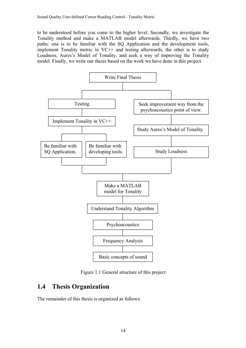
1.3 Working Process Our work has progressed as illustrated in the figure below when read in a bottom-up manner. Firstly, we build our knowledge from the basic concepts of sound, frequency analysis and psychoacoustics, which are related in a way that lower level is necessary
13
Sound Quality User-defined Cursor Reading Control - Tonality Metric
to be understood before you come to the higher level. Secondly, we investigate the Tonality method and make a MATLAB model afterwards. Thirdly, we have two paths: one is to be familiar with the SQ Application and the development tools, implement Tonality metric in VC++ and testing afterwards, the other is to study Loudness, Aures’s Model of Tonality, and seek a way of improving the Tonality model. Finally, we write our thesis based on the work we have done in this project.
Implement Tonality in VC++
Be familiar with SQ Application.
Be familiar with developing tools.
Make a MATLAB model for Tonality
Seek improvement way from the psychoacoustics point of view.
Psychoacoustics
Frequency Analysis
Basic concepts of sound
Write Final Thesis
Study Loudness
Study Aures’s Model of Tonality
Understand Tonality Algorithm
Testing
Figure 1.1 General structure of this project 1.4 Thesis Organization The remainder of this thesis is organized as follows:
14

Sound Quality User-defined Cursor Reading Control - Tonality Metric
Chapter 2 provides the specific background knowledge about Sound Quality, Psychoacoustics and Sound Quality metrics, which are necessary to know in order to understand this thesis. Chapter 3 reviews the original Tonality Algorithm presented in 1982 by Terhardt, E., Stoll,G., and Seewann, M. Chapter 4 describes how we built Tonality Model in MATLAB according to Terhardt’s method. Chapter 5 describes the technical and practical information in the progress of the implementation of Tonality metric for B&K SQ Application in VC++. Chapter 6 shows how we test our MATLAB and VC++ programs. Chapter 7 includes some theoretic study in Stationary Loudness and Aures’s Model of Tonality. Chapter 8 summarizes our work and indicates future implementation paths. Additionally, source code, test data and relevant materials of this project are available in Appendix. Chapter 2 Specific Background Knowledge for this Thesis According to the specific area of this project, we would like to present the background knowledge before we go into our thesis work in detail. This chapter covers the basic
15
Sound Quality User-defined Cursor Reading Control - Tonality Metric
concepts of Sound Quality and psychoacoustics, the metrics involved in Sound Quality field, the feature of Tonality metric, and some basic concepts. Most of the content in this chapter is taken from the relevant B&K Sound Quality Lecture Notes and it can be studied as an infrastructure of the whole thesis. 2.1 Sound Quality
2.1.1 What is Sound Quality? The sound of a product is now a product parameter that needs the same attention as its physical design, horsepower, color, weight, price etc. It all started in the automotive industry more than 10 years ago and it is still in that area that the most advanced Sound Quality developments take place. One reason is the very heavy competition between car manufacturers and the fact that most cars are of high quality and have the same performance in relation to what they are supposed to do. Sound Quality as a relatively new product parameter has then become an important item to compete on. If your car has better Sound Quality than the competition you are closer to win the sale. In recent years the focus on Sound Quality has spread to almost all other industries producing products that makes noise. The household appliance industries are good examples. Sound Quality as a product parameter is most developed in USA, Europe and Japan. In other countries is expected to grow rapidly as more and more products become not sellable unless their Sound Quality parameters has been attended to. As product sound is directly communicating with the users senses – the ears – the knowledge of how we perceive sound has got increased focus. This discipline is called Psychoacoustics and is important in the education of design and development engineers.
2.1.2 Why improve the Quality of Sound? The noise from a product is a part of the communication between the product and its user. Therefore it has to be changed into sound that is pleasing to the user and give him all the information of the function and life time of the product he needs - no more no less. The pleasing aspect of product sound is perceived subjectively and depends on the individual user. This situation leaves the designer of the product in a very challenging position. He has to optimise the product sound to the target customer group that has a taste that is not uniform and will change over time as fashion. Pleasing sounds get worn and need replacement by new exciting sounds. He has to skip old design tools and learn new ones. For example the widely used A-weighting is fine for noise but useless for sound. Three different vacuum cleaners may have the same A-weighted noise level but can have very different sounds. No noise may be a target for a noise control, but in relation to Sound Quality no sound is unacceptable. Products should always signal proper operation to the user as well as a warning signal when the electric drill is overloaded or the car is hitting rough road surface an the driver should reduce speed.
2.1.3 Work with Sound Quality
16
Sound Quality User-defined Cursor Reading Control - Tonality Metric
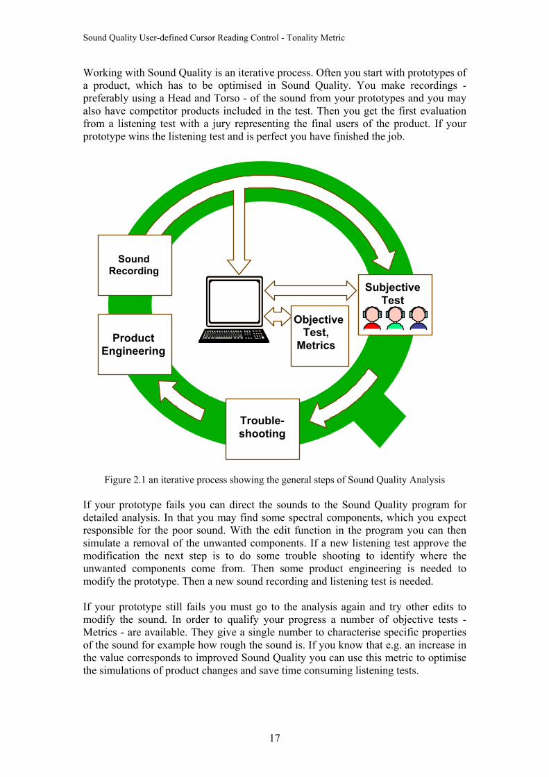
Working with Sound Quality is an iterative process. Often you start with prototypes of a product, which has to be optimised in Sound Quality. You make recordings - preferably using a Head and Torso - of the sound from your prototypes and you may also have competitor products included in the test. Then you get the first evaluation from a listening test with a jury representing the final users of the product. If your prototype wins the listening test and is perfect you have finished the job.
ObjectiveTest,
Metrics
Sound Recording
Subjective Test
Product Engineering
Trouble-shooting
Figure 2.1 an iterative process showing the general steps of Sound Quality Analysis If your prototype fails you can direct the sounds to the Sound Quality program for detailed analysis. In that you may find some spectral components, which you expect responsible for the poor sound. With the edit function in the program you can then simulate a removal of the unwanted components. If a new listening test approve the modification the next step is to do some trouble shooting to identify where the unwanted components come from. Then some product engineering is needed to modify the prototype. Then a new sound recording and listening test is needed. If your prototype still fails you must go to the analysis again and try other edits to modify the sound. In order to qualify your progress a number of objective tests - Metrics - are available. They give a single number to characterise specific properties of the sound for example how rough the sound is. If you know that e.g. an increase in the value corresponds to improved Sound Quality you can use this metric to optimise the simulations of product changes and save time consuming listening tests.
17
Sound Quality User-defined Cursor Reading Control - Tonality Metric
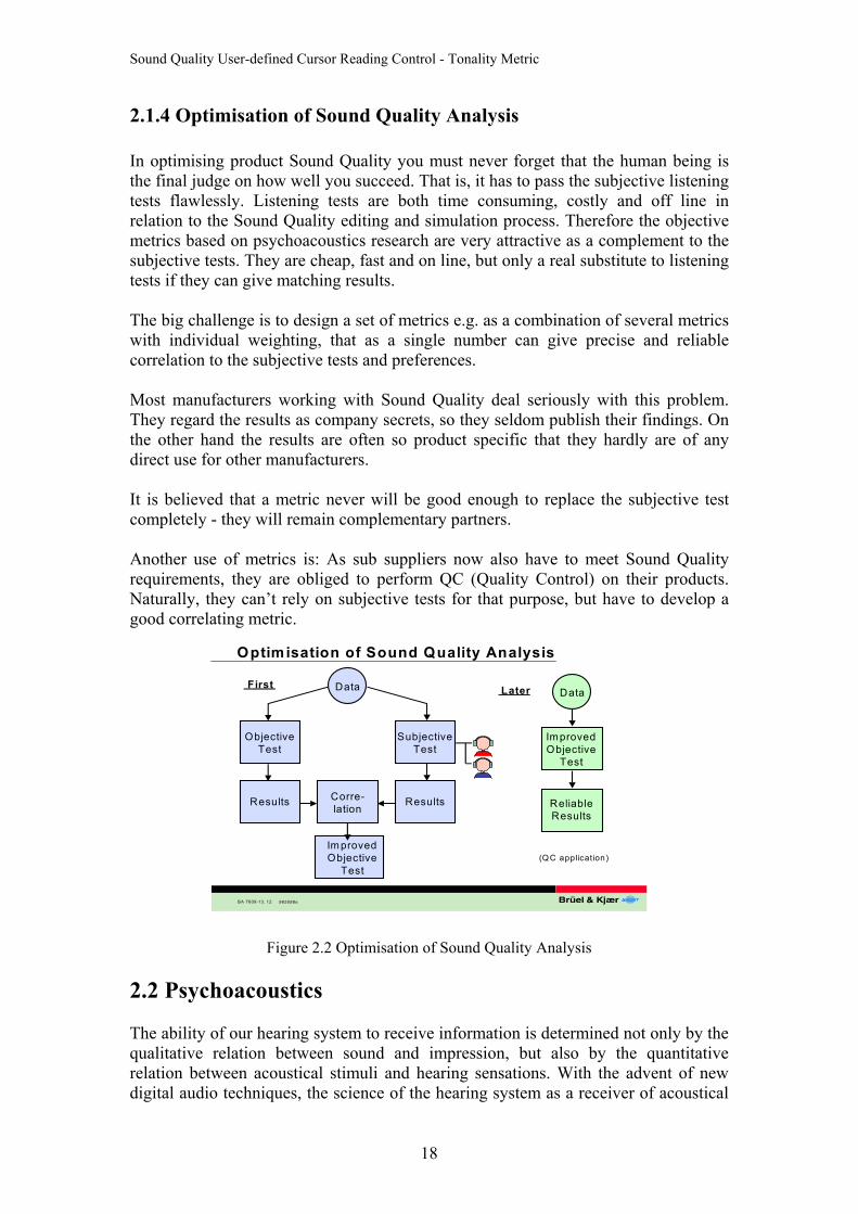
2.1.4 Optimisation of Sound Quality Analysis In optimising product Sound Quality you must never forget that the human being is the final judge on how well you succeed. That is, it has to pass the subjective listening tests flawlessly. Listening tests are both time consuming, costly and off line in relation to the Sound Quality editing and simulation process. Therefore the objective metrics based on psychoacoustics research are very attractive as a complement to the subjective tests. They are cheap, fast and on line, but only a real substitute to listening tests if they can give matching results. The big challenge is to design a set of metrics e.g. as a combination of several metrics with individual weighting, that as a single number can give precise and reliable correlation to the subjective tests and preferences. Most manufacturers working with Sound Quality deal seriously with this problem. They regard the results as company secrets, so they seldom publish their findings. On the other hand the results are often so product specific that they hardly are of any direct use for other manufacturers. It is believed that a metric never will be good enough to replace the subjective test completely - they will remain complementary partners. Another use of metrics is: As sub suppliers now also have to meet Sound Quality requirements, they are obliged to perform QC (Quality Control) on their products. Naturally, they can’t rely on subjective tests for that purpose, but have to develop a good correlating metric.
BA 7609-13, 12
ImprovedObjective
Test
Optimisation of Sound Quality Analysis
ObjectiveTest
Results
ImprovedObjective
Test
Data
SubjectiveTest
ResultsCorre-lation Reliable
Results
Data
(Q C application)
LaterFirst
965088e
Figure 2.2 Optimisation of Sound Quality Analysis 2.2 Psychoacoustics The ability of our hearing system to receive information is determined not only by the qualitative relation between sound and impression, but also by the quantitative relation between acoustical stimuli and hearing sensations. With the advent of new digital audio techniques, the science of the hearing system as a receiver of acoustical
18
Sound Quality User-defined Cursor Reading Control - Tonality Metric
information, i.e. the science of psychoacoustics, has gained additional importance. In the years from 1952 to 1967, the research group on hearing phenomena at the Institute of Telecommunications in Stuttgart made important contributions to the quantitative correlation of acoustical stimuli and hearing sensations, i.e. to psychoacoustics. Since 1967, research groups at the Institute of Electroacoustics in Munich have continued to make progress in this field. The correlation between acoustical stimuli and hearing sensations is investigated both by acquiring sets of experimental data and by models which simulate the measured facts in an understandable way.
2.2.1 Stimuli and Sensations The most important physical magnitude for psychoacoustics is the time function of sound pressure. The stimulus can be described by physical means in terms of sound pressure level, frequency, duration and so on. The physical magnitudes mentioned are correlated with the psychophysical magnitudes loudness, pitch, and subjective duration, which are called hearing sensations. However, it should be mentioned that the pitch of a pure tone depends not only on its frequency, but also to some extent on its level. Nonetheless, the main correlation of the hearing sensation pitch is the stimulus quantity frequency. Physical stimuli only lead to hearing sensations if their physical magnitudes lie within the range relevant for the hearing organ. For example, frequencies below 20Hz and above about 20kHz do not lead to a hearing sensation whatever their stimulus magnitude. Just as we can describe a stimulus by separate physical characteristics, we can also consider several hearing sensations separately. For instance, we can state, “the tone with the higher pitch was louder than the tone with the lower pitch”. This means that we can attend separately to the hearing sensation “loudness” on one hand and “pitch” on the other. A major goal of psychoacoustics is to arrive at sensation magnitudes analogous to stimulus magnitudes. For example, we can state that a 1-kHz tone with 20mPa sound pressure produces a loudness of 4sone in terms of hearing sensation. The unit “sone” is used for the hearing sensation loudness in just the same way as the unit “Pa” is used for the sound pressure. It is most important not to mix up stimulus magnitudes such as “Pa” or “dB” and sensation magnitudes such as “sone”. [2.1]
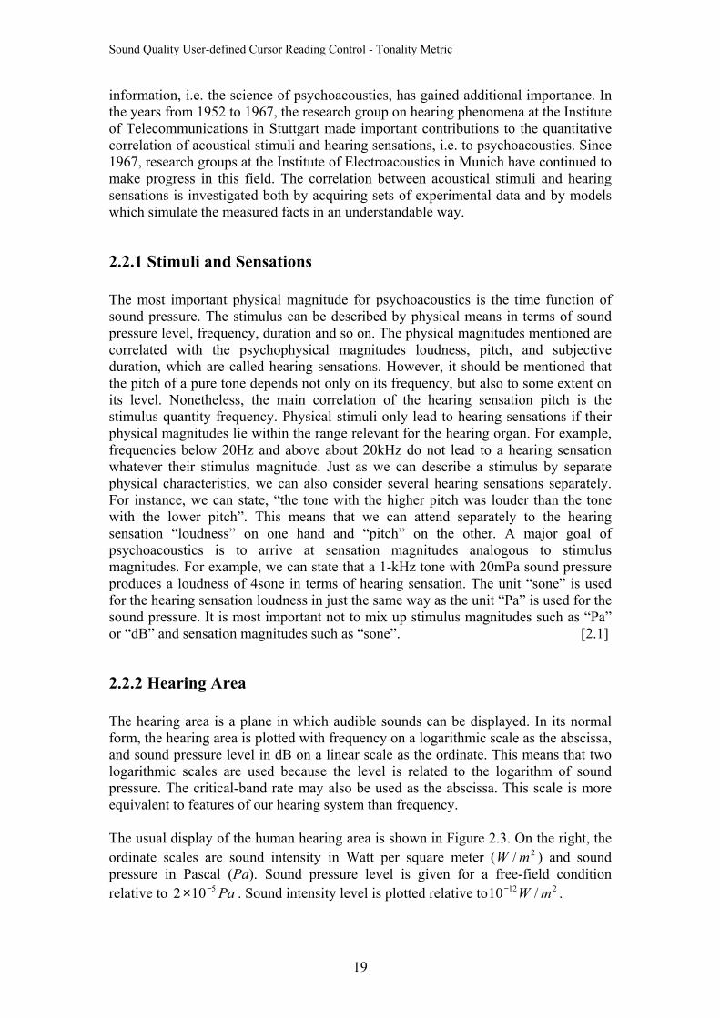
2.2.2 Hearing Area The hearing area is a plane in which audible sounds can be displayed. In its normal form, the hearing area is plotted with frequency on a logarithmic scale as the abscissa, and sound pressure level in dB on a linear scale as the ordinate. This means that two logarithmic scales are used because the level is related to the logarithm of sound pressure. The critical-band rate may also be used as the abscissa. This scale is more equivalent to features of our hearing system than frequency. The usual display of the human hearing area is shown in Figure 2.3. On the right, the ordinate scales are sound intensity in Watt per square meter (W ) and sound pressure in Pascal (Pa). Sound pressure level is given for a free-field condition relative to . Sound intensity level is plotted relative to10 .
2/ m
12 /W−Pa5102 −× 2m
19
Sound Quality User-defined Cursor Reading Control - Tonality Metric
BA 7615-13, 3
Auditory Field
960423
140dB
120
100
80
60
40
20
0
0.02 0.05 0.1 0.2 0.5 1 2 5 10 20 kHz Frequency
Soun
d In
tens
ity L
evel
Soun
d Pr
essu
re L
evel
Thresholdin Quiet
Limit of Damage Risk
Threshold of Pain
Speech
Music
140dB
120
100
80
60
40
20
0
100
W
1
10-2
10-4
10-6
10-8
10-10
10-12
200
Pa
20
2
0.2
2·10-2
2·10-3
2·10-4
2·10-5
m2
Soun
d In
tens
ity
Soun
d Pr
essu
re
Figure 2.3 Hearing areas between threshold in quiet and threshold of pain. This display of the auditory field illustrates the limits of the human auditory system. The solid line denotes, as a lower limit, the threshold in quiet for a pure tone to be just audible. The upper dashed line represents the threshold of pain. However if the Limit of Damage Risk is exceeded for a longer time, permanent hearing loss may occur. This could lead to an increase in the threshold of hearing as illustrated by the dashed curve in the lower right-hand corner. Normal speech and music have levels in the shaded areas, while higher levels require electronic amplification. Human hearing is extremely sensitive. An acoustic power intensity of only 1 mW per square metre may already exceed the limit of damage risk.
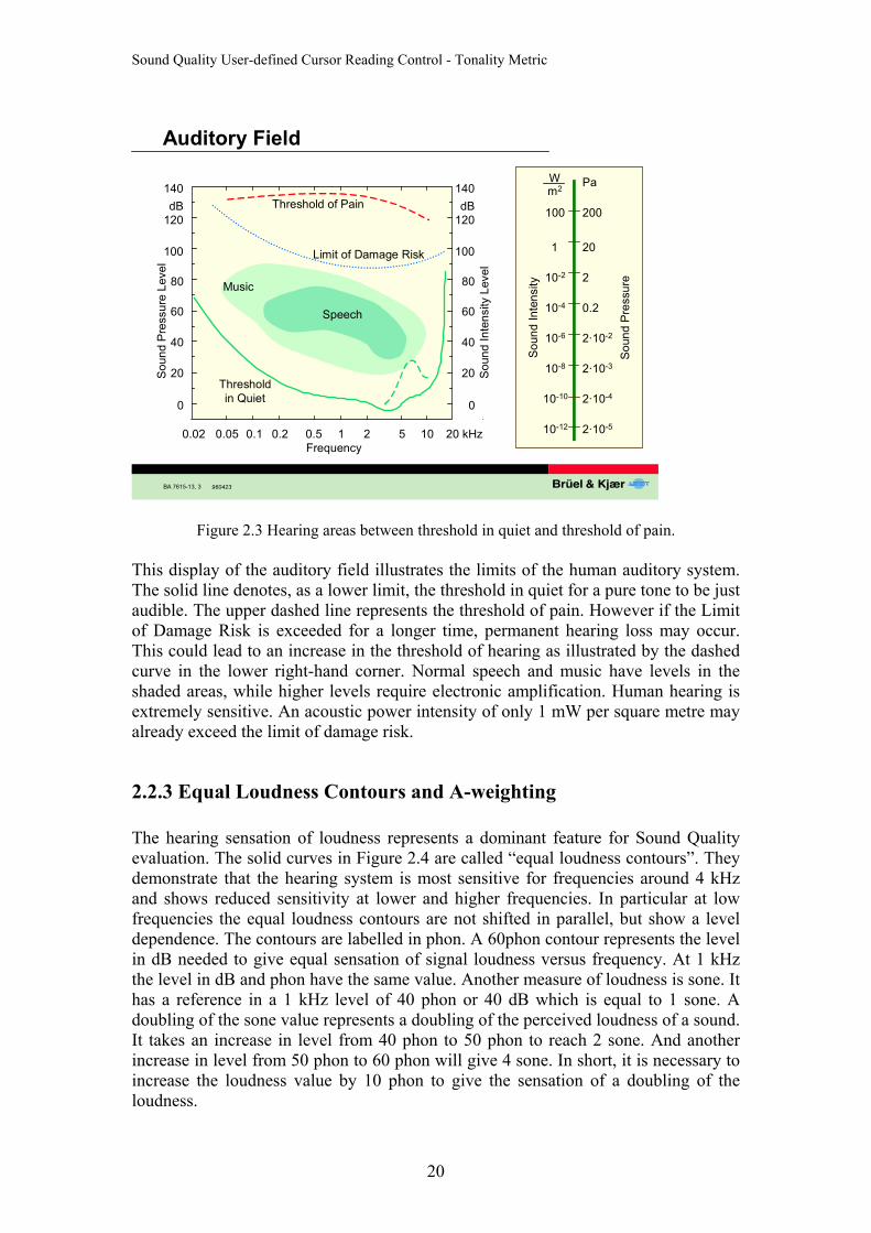
2.2.3 Equal Loudness Contours and A-weighting The hearing sensation of loudness represents a dominant feature for Sound Quality evaluation. The solid curves in Figure 2.4 are called “equal loudness contours”. They demonstrate that the hearing system is most sensitive for frequencies around 4 kHz and shows reduced sensitivity at lower and higher frequencies. In particular at low frequencies the equal loudness contours are not shifted in parallel, but show a level dependence. The contours are labelled in phon. A 60phon contour represents the level in dB needed to give equal sensation of signal loudness versus frequency. At 1 kHz the level in dB and phon have the same value. Another measure of loudness is sone. It has a reference in a 1 kHz level of 40 phon or 40 dB which is equal to 1 sone. A doubling of the sone value represents a doubling of the perceived loudness of a sound. It takes an increase in level from 40 phon to 50 phon to reach 2 sone. And another increase in level from 50 phon to 60 phon will give 4 sone. In short, it is necessary to increase the loudness value by 10 phon to give the sensation of a doubling of the loudness.
20
Sound Quality User-defined Cursor Reading Control - Tonality Metric
The dashed curve in the graph shows the well-known A-weighting. For very low sounds there is a good agreement with the 20 phon curve. At higher levels, e.g., 80 phon - typical for everyday sounds - it underestimates the loudness of their low frequency components.
BA 7615-13, 12
Equal Loudness Contours and A-weighting
960432
100
fT
LT
dB80
60
40
20
20 50 100 200 500 1 k 2 k 5 k 10 k 20 kHz
20
40
LN = 60phon
80
100
1 sone
4 sone
16 sone
2 sone
8 sone
A-weighting
Figure 2.4 equal Loudness Contours and A-weighting
2.2.4 Masking Masking plays a very important role in everyday life. For a conversation on the pavements of a quiet street, for example, little speech power is necessary for the speakers to understand each other. However, if a loud truck passes by, our conversation is severely disturbed: by keeping the speech power constant, our partner can no longer hear us. There are two ways of overcoming this phenomenon of masking. We can either wait until the truck passed and then continue our conversation, or we can raise our voice to produce more speech power and greater loudness. Our partner then can hear the speech sound again. Similar effects take place in most pieces of music. One instrument may be masked by another if one of them produces high levels while the other remains faint. If the loud instrument pauses, the faint one becomes audible again. These are typical examples of simultaneous masking. To measure the effect of masking quantitatively, the masked threshold is usually determined. The masked threshold is the sound pressure level of a test sound (usually a sinusoidal test tone), necessary to be just audible in the presence of a masker. Masked threshold, in all but a very few special cases, always lies above threshold in quiet; it is identical with threshold in quiet when the frequencies of the masker and the test sound are very different.
21
Sound Quality User-defined Cursor Reading Control - Tonality Metric
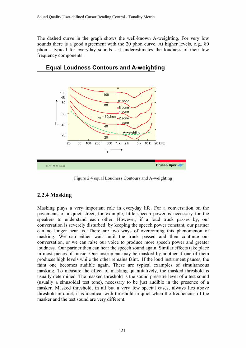
If the masker is increased steadily, there is a continuous transition between an audible (unmasked) test tone and one that is totally masked. This means that besides total masking, partial masking also occurs. Partial masking reduces the loudness of a test tone but does not mask the test tone completely. This effect often takes place in conversations. Partial masking is related to a reduction in loudness. Masking effects can be measured not only when masker and test sound are presented simultaneously, but also when they are not simultaneous. In the latter case, the test sound has to be a short burst or sound impulse, which can be presented before the masker stimulus is switched on. The masking effect produced under these conditions is called pre-stimulus masking, shorted to “premasking” (the expression “backward masking” is also used). This effect is not very strong, but if the test sound is presented after the masker is switched off, then quite pronounced effects occur. Because the test sound is presented after the termination of the masker, the effect is called post-stimulus masking, shorted to “postmasking” (the expression “forward masking” is also used), as shown in Figure 2.5.
Figure 2.5 per (backward) and post- (forward) masking Masking represents one of the most basic effects in psychoacoustics. This is normally determined as the audibility of pure tones in the presence of masking sounds. Different kinds of noises are commonly used in psychoacoustics as masker noises when investigating masking patterns.
22
Sound Quality User-defined Cursor Reading Control - Tonality Metric
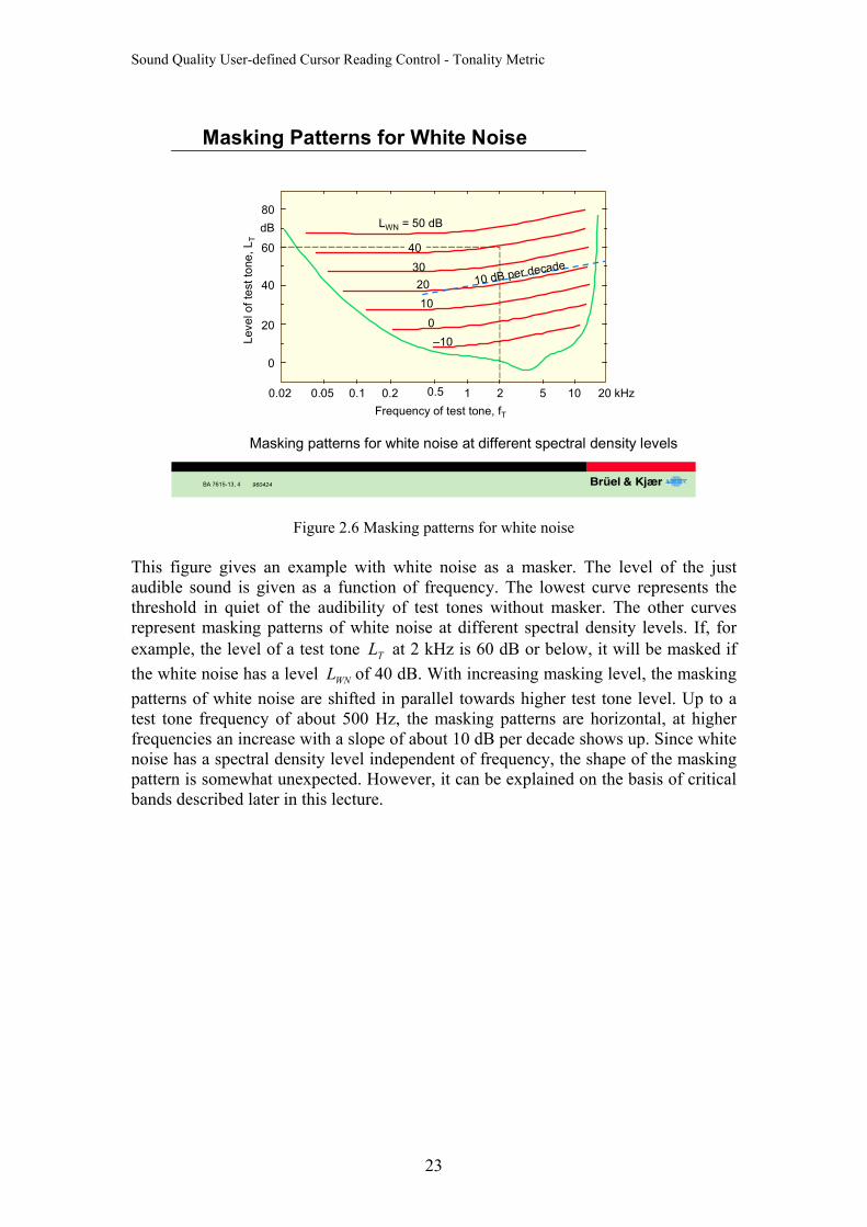
BA 7615-13, 4
Masking Patterns for White Noise
960424
Masking patterns for white noise at different spectral density levels
80dB
60
40
20
0
0.02 0.05 0.1 0.2 0.5 1 2 10 20 kHzFrequency of test tone, fT
Leve
l of t
est t
one,
LT
–100
1020
3010 dB per decade
5
40
LWN = 50 dB
Figure 2.6 Masking patterns for white noise This figure gives an example with white noise as a masker. The level of the just audible sound is given as a function of frequency. The lowest curve represents the threshold in quiet of the audibility of test tones without masker. The other curves represent masking patterns of white noise at different spectral density levels. If, for example, the level of a test tone at 2 kHz is 60 dB or below, it will be masked if the white noise has a level of 40 dB. With increasing masking level, the masking patterns of white noise are shifted in parallel towards higher test tone level. Up to a test tone frequency of about 500 Hz, the masking patterns are horizontal, at higher frequencies an increase with a slope of about 10 dB per decade shows up. Since white noise has a spectral density level independent of frequency, the shape of the masking pattern is somewhat unexpected. However, it can be explained on the basis of critical bands described later in this lecture.
TL
WNL
23
Sound Quality User-defined Cursor Reading Control - Tonality Metric
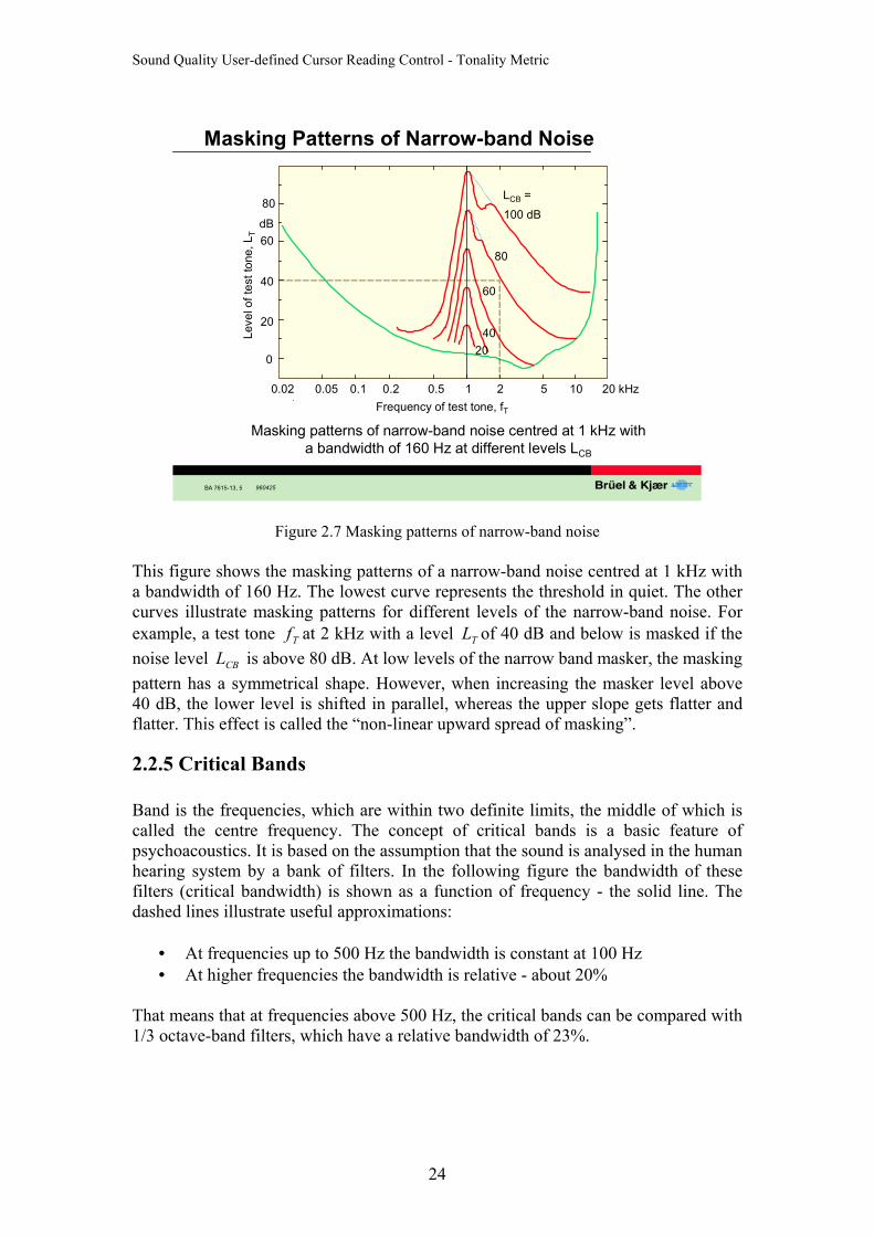
BA 7615-13, 5
Masking Patterns of Narrow-band Noise
960425
80
dB60
40
20
0
0.02 0.05 0.1 0.2 0.5 1 2 5 10 20 kHz
2040
60
80
100 dBLCB =
Masking patterns of narrow-band noise centred at 1 kHz witha bandwidth of 160 Hz at different levels LCB
Frequency of test tone, fT
Leve
l of t
est t
one,
LT
Figure 2.7 Masking patterns of narrow-band noise This figure shows the masking patterns of a narrow-band noise centred at 1 kHz with a bandwidth of 160 Hz. The lowest curve represents the threshold in quiet. The other curves illustrate masking patterns for different levels of the narrow-band noise. For example, a test tone at 2 kHz with a level of 40 dB and below is masked if the noise level is above 80 dB. At low levels of the narrow band masker, the masking pattern has a symmetrical shape. However, when increasing the masker level above 40 dB, the lower level is shifted in parallel, whereas the upper slope gets flatter and flatter. This effect is called the “non-linear upward spread of masking”.
Tf TL
CBL
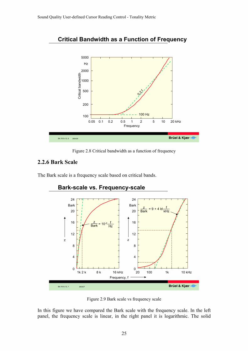
2.2.5 Critical Bands Band is the frequencies, which are within two definite limits, the middle of which is called the centre frequency. The concept of critical bands is a basic feature of psychoacoustics. It is based on the assumption that the sound is analysed in the human hearing system by a bank of filters. In the following figure the bandwidth of these filters (critical bandwidth) is shown as a function of frequency - the solid line. The dashed lines illustrate useful approximations:
• At frequencies up to 500 Hz the bandwidth is constant at 100 Hz • At higher frequencies the bandwidth is relative - about 20%
That means that at frequencies above 500 Hz, the critical bands can be compared with 1/3 octave-band filters, which have a relative bandwidth of 23%.
24
Sound Quality User-defined Cursor Reading Control - Tonality Metric
BA 7615-13, 6
Critical Bandwidth as a Function of Frequency
960426
5000
Hz
2000
1000
500
200
0.05 0.1 0.2 0.5 1 2 5 10 20 kHzFrequency
Crit
ical
ban
dwid
th
100 Hz
0.2 f
100
Figure 2.8 Critical bandwidth as a function of frequency
2.2.6 Bark Scale The Bark scale is a frequency scale based on critical bands.
BA 7615-13, 7
Bark-scale vs. Frequency-scale
960427
24
Bark
20
16
12
8
1k 2 k 8 k 16 kHz 20 100 1k 10 kHzFrequency, f
z
4
0
zBark = 10-2 f
Hz
zBark
= 9 + 4 ld fkHz
24
Bark
20
16
12
8
z
4
0
Figure 2.9 Bark scale vs frequency scale
In this figure we have compared the Bark scale with the frequency scale. In the left panel, the frequency scale is linear, in the right panel it is logarithmic. The solid
25
Sound Quality User-defined Cursor Reading Control - Tonality Metric
curves describe the relation between the Bark scale and the frequency scale. The dashed curves show the useful approximations. These are valid up to 500 Hz left panel, and above 500 Hz right panel. Examples of relation between Bark and frequency values:
• A frequency of 200 Hz corresponds to 2 Bark • A frequency of 2 kHz corresponds to 13 Bark • Bark band 1 covers the frequency range from 0 - 100 Hz • Bark band 24 covers the frequency range from 12000 - 15500 Hz
The name “Bark” is chosen in honour of the late famous acoustician Barkhausen from Dresden.
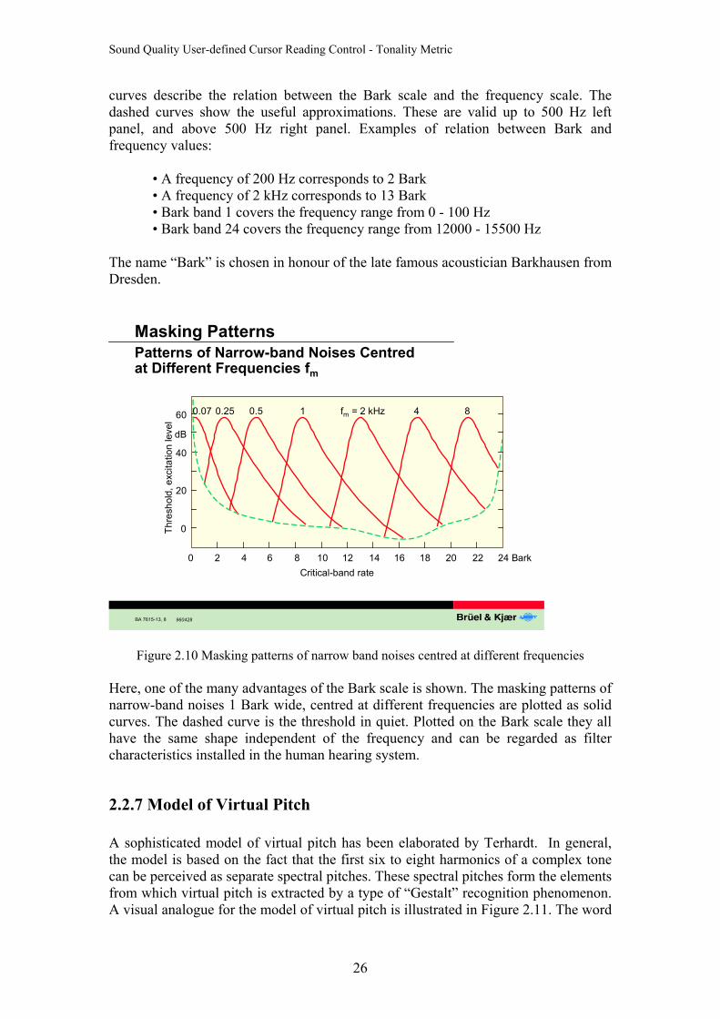
BA 7615-13, 8
Masking Patterns
960428
60
dB
40
20
0
0 2 4Critical-band rate
8 10 12 14 16 18 20 24 Bark
Thre
shol
d, e
xcita
tion
leve
l
6 22
0.250.07 0.5 1 fm = 2 kHz 4 8
Patterns of Narrow-band Noises Centredat Different Frequencies fm
Figure 2.10 Masking patterns of narrow band noises centred at different frequencies Here, one of the many advantages of the Bark scale is shown. The masking patterns of narrow-band noises 1 Bark wide, centred at different frequencies are plotted as solid curves. The dashed curve is the threshold in quiet. Plotted on the Bark scale they all have the same shape independent of the frequency and can be regarded as filter characteristics installed in the human hearing system.
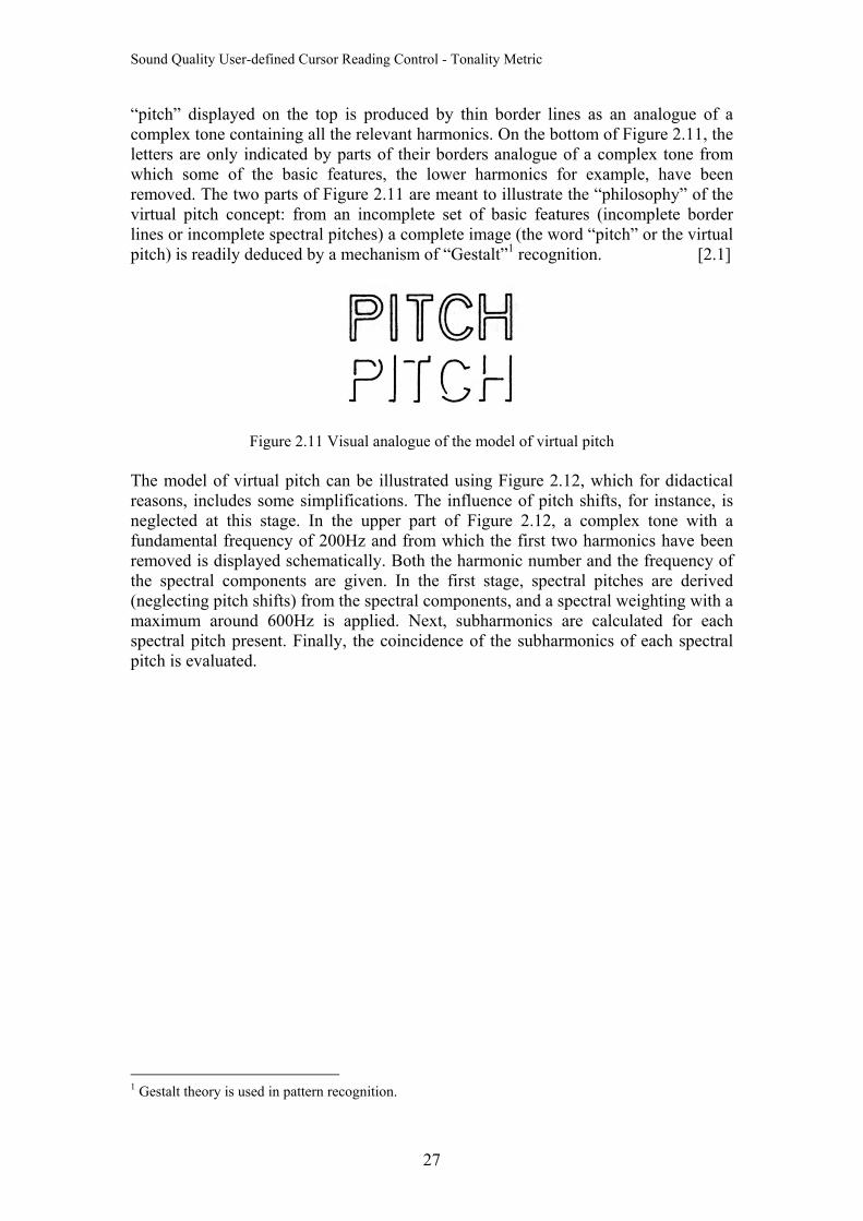
2.2.7 Model of Virtual Pitch A sophisticated model of virtual pitch has been elaborated by Terhardt. In general, the model is based on the fact that the first six to eight harmonics of a complex tone can be perceived as separate spectral pitches. These spectral pitches form the elements from which virtual pitch is extracted by a type of “Gestalt” recognition phenomenon. A visual analogue for the model of virtual pitch is illustrated in Figure 2.11. The word
26
Sound Quality User-defined Cursor Reading Control - Tonality Metric
“pitch” displayed on the top is produced by thin border lines as an analogue of a complex tone containing all the relevant harmonics. On the bottom of Figure 2.11, the letters are only indicated by parts of their borders analogue of a complex tone from which some of the basic features, the lower harmonics for example, have been removed. The two parts of Figure 2.11 are meant to illustrate the “philosophy” of the virtual pitch concept: from an incomplete set of basic features (incomplete border lines or incomplete spectral pitches) a complete image (the word “pitch” or the virtual pitch) is readily deduced by a mechanism of “Gestalt”1 recognition. [2.1]
Figure 2.11 Visual analogue of the model of virtual pitch
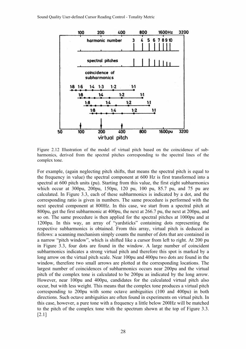
The model of virtual pitch can be illustrated using Figure 2.12, which for didactical reasons, includes some simplifications. The influence of pitch shifts, for instance, is neglected at this stage. In the upper part of Figure 2.12, a complex tone with a fundamental frequency of 200Hz and from which the first two harmonics have been removed is displayed schematically. Both the harmonic number and the frequency of the spectral components are given. In the first stage, spectral pitches are derived (neglecting pitch shifts) from the spectral components, and a spectral weighting with a maximum around 600Hz is applied. Next, subharmonics are calculated for each spectral pitch present. Finally, the coincidence of the subharmonics of each spectral pitch is evaluated.
1 Gestalt theory is used in pattern recognition.
27
Sound Quality User-defined Cursor Reading Control - Tonality Metric
Figure 2.12 Illustration of the model of virtual pitch based on the coincidence of sub-harmonics, derived from the spectral pitches corresponding to the spectral lines of the complex tone. For example, (again neglecting pitch shifts, that means the spectral pitch is equal to the frequency in value) the spectral component at 600 Hz is first transformed into a spectral at 600 pitch units (pu). Starting from this value, the first eight subharmonics which occur at 300pu, 200pu, 150pu, 120 pu, 100 pu, 85.7 pu, and 75 pu are calculated. In Figure 3.3, each of these subharmonics is indicated by a dot, and the corresponding ratio is given in numbers. The same procedure is performed with the next spectral component at 800Hz. In this case, we start from a spectral pitch at 800pu, get the first subharmonic at 400pu, the next at 266.7 pu, the next at 200pu, and so on. The same procedure is then applied for the spectral pitches at 1000pu and at 1200pu. In this way, an array of “yardsticks” containing dots representing the respective subharmonics is obtained. From this array, virtual pitch is deduced as follows: a scanning mechanism simply counts the number of dots that are contained in a narrow “pitch window”, which is shifted like a cursor from left to right. At 200 pu in Figure 3.3, four dots are found in the window. A large number of coincident subharmonics indicates a strong virtual pitch and therefore this spot is marked by a long arrow on the virtual pitch scale. Near 100pu and 400pu two dots are found in the window, therefore two small arrows are plotted at the corresponding locations. The largest number of coincidences of subharmonics occurs near 200pu and the virtual pitch of the complex tone is calculated to be 200pu as indicated by the long arrow. However, near 100pu and 400pu, candidates for the calculated virtual pitch also occur, but with less weight. This means that the complex tone produces a virtual pitch corresponding to 200pu with some octave ambiguities (100 and 400pu) in both directions. Such octave ambiguities are often found in experiments on virtual pitch. In this case, however, a pure tone with a frequency a little below 200Hz will be matched to the pitch of the complex tone with the spectrum shown at the top of Figure 3.3. [2.1]
28
Sound Quality User-defined Cursor Reading Control - Tonality Metric
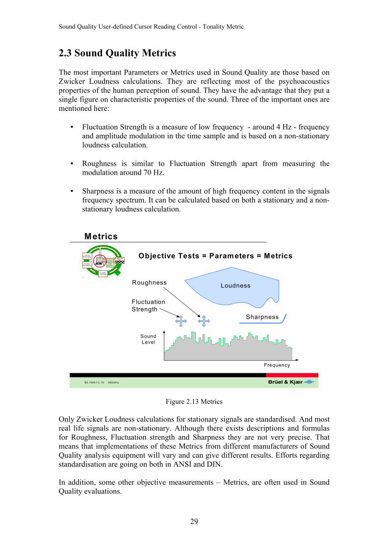
2.3 Sound Quality Metrics The most important Parameters or Metrics used in Sound Quality are those based on Zwicker Loudness calculations. They are reflecting most of the psychoacoustics properties of the human perception of sound. They have the advantage that they put a single figure on characteristic properties of the sound. Three of the important ones are mentioned here:
• Fluctuation Strength is a measure of low frequency - around 4 Hz - frequency and amplitude modulation in the time sample and is based on a non-stationary loudness calculation.
• Roughness is similar to Fluctuation Strength apart from measuring the
modulation around 70 Hz.
• Sharpness is a measure of the amount of high frequency content in the signals frequency spectrum. It can be calculated based on both a stationary and a non-stationary loudness calculation.
BA 7609-13, 10
FluctuationStrength
Metrics
Sharpness
LoudnessRoughness
Objective Tests = Parameters = Metrics
Frequency
SoundLevel
965087e
ObjectiveTest,
Metrics
SubjectiveTest
ProductEngineering
Trouble-shooting
SoundQ uality
Program
SoundRecording
Figure 2.13 Metrics Only Zwicker Loudness calculations for stationary signals are standardised. And most real life signals are non-stationary. Although there exists descriptions and formulas for Roughness, Fluctuation strength and Sharpness they are not very precise. That means that implementations of these Metrics from different manufacturers of Sound Quality analysis equipment will vary and can give different results. Efforts regarding standardisation are going on both in ANSI and DIN. In addition, some other objective measurements – Metrics, are often used in Sound Quality evaluations.
29
Sound Quality User-defined Cursor Reading Control - Tonality Metric
• Pleasantness and Annoyance are combination Metrics based on a weighted
sum of Zwicker Loudness, Fluctuation Strength, Roughness and Sharpness. • Tone to Noise Ratio is a measure describing the amount of pure tones in the
signal
• Prominence ratio is a description of the amount of noise in a critical band in relation to the noise in the adjacent bands.
• Tonality or Pitch is a measure of how strong the sensation of “frequency” is in
a complex signal.
• Speech Interference Level, Articulation Index and Speech Transmission index are all measures related to the quality of a speech transmission channel. They also find uses in some Sound Quality applications.
• Kurtosis is a measure of impulsiveness of the time signal. Basically it sums up
all time samples level differences from the signals mean value and raised to the power of 4 and then normalised. The method exaggerates the impulses in the sound and a high kurtosis value normally reflects poor Sound Quality.
2.4 Tonality Metric Tonality is an important parameter affecting Sound Quality. The perceived tonal character of sounds plays an important role both in Sound Quality research and in the study of annoyance through noise. Tonality is not standardized yet so different companies have their own version of implementation. Tonality calculation is based on pitch-extraction algorithm described by Terhardt. The algorithm provides two pitch patterns: the spectral-pitch pattern and the virtual-pitch pattern, each of which consists of pitch values and pitch weights. For more information about the algorithm, please refer to Chapter 3. 2.5 Terms and Definitions Before going into detail of the following sections, it is worth noting some of the basic concepts used in the Sound Quality field. • Attenuation Reduction in magnitude of a physical quantity such as sound, either by electronic means or by a physical barrier, including various absorptive materials. • Amplitude The instantaneous magnitude of an oscillating quantity such as sound pressure. The peak amplitude is the maximum value.
30
Sound Quality User-defined Cursor Reading Control - Tonality Metric
• Band Frequencies, which are within two definite limits, the middle of which is called the centre frequency. • Bandwidth The difference between the highest and lowest frequencies of a band, sometimes expressed in standard sizes, such as octave, half-octave, third-octave. • Central frequency The frequency in the middle of a Band of frequencies, by which the band is identified together with the Bandwidth. • Constant percentage Bands (CPB) CPB means constant percentage bandwidth. It is a way of displaying data in octave form – in Sound Quality’s case 1/3-octave spacing. • Decibel (dB) The decibel is not an absolute unit of measurement. It is a ratio between a measured quantity and an agreed reference level. The dB scale is logarithmic and uses the hearing threshold of 20 µ Pa as the reference level. This is defined as 0 dB. The advantage of using dB’s is that it converts the linear scale with large and unwieldy numbers into a much more manageable scale from 0 dB at the threshold of hearing (20 µ Pa) to 130 dB at the threshold of pain. • Diffuse field The sound is assumed to reach the listener’s ears from all directions at the same intensity. This condition is approximated in an ordinary room. The method is applicable to all types of spectra and also is based on the assumption that the sound is steady rather than intermittent. • Fast Fourier Transform (FFT) The Fast Fourier Transform is an algorithm or calculation procedure for obtaining the Discrete Fourier Transform (DFT) with a greatly reduced number of arithmetic operations compared with a direct evaluation. Since its first publication in 1965 it has revolutionized the field of signal analysis, and it is still probably the most important single analysis technique available.
31
Sound Quality User-defined Cursor Reading Control - Tonality Metric
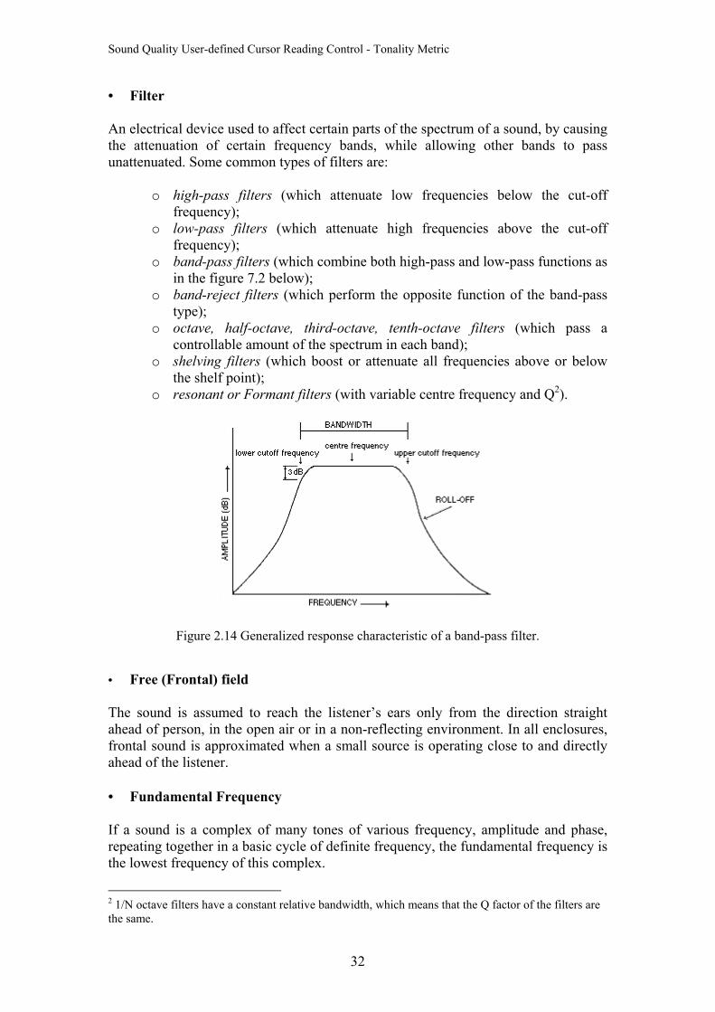
• Filter An electrical device used to affect certain parts of the spectrum of a sound, by causing the attenuation of certain frequency bands, while allowing other bands to pass unattenuated. Some common types of filters are:
o high-pass filters (which attenuate low frequencies below the cut-off frequency);
o low-pass filters (which attenuate high frequencies above the cut-off frequency);
o band-pass filters (which combine both high-pass and low-pass functions as in the figure 7.2 below);
o band-reject filters (which perform the opposite function of the band-pass type);
o octave, half-octave, third-octave, tenth-octave filters (which pass a controllable amount of the spectrum in each band);
o shelving filters (which boost or attenuate all frequencies above or below the shelf point);
o resonant or Formant filters (with variable centre frequency and Q2).
Figure 2.14 Generalized response characteristic of a band-pass filter. • Free (Frontal) field
The sound is assumed to reach the listener’s ears only from the direction straight ahead of person, in the open air or in a non-reflecting environment. In all enclosures, frontal sound is approximated when a small source is operating close to and directly ahead of the listener. • Fundamental Frequency If a sound is a complex of many tones of various frequency, amplitude and phase, repeating together in a basic cycle of definite frequency, the fundamental frequency is the lowest frequency of this complex.
2 1/N octave filters have a constant relative bandwidth, which means that the Q factor of the filters are the same.
32
Sound Quality User-defined Cursor Reading Control - Tonality Metric
• Harmonic A harmonic tone consists of a sum of pure tones (each one called a partial), whose frequencies are in integer ratios of 1, 2, 3, ... Partials related in this way are called the harmonics of the tone. • Hertz The unit of frequency measurement, representing cycles per second. • Loudness Subjective impression of the intensity of a sound. • Masking The process by which threshold of audibility of one sound is raised by the presence of another (masking) sound. • Narrow band noise Sound classed as noise, which has its energy distributed over a relatively small section of the audible range. • Octave An octave is a doubling or halving of frequency. 20Hz-40Hz is often considered the bottom octave. • One Octave bands Frequency ranges in which the upper limit of each band is twice the lower limit and Octave bands are identified by their geometric mean frequency, or centre frequency. • One-third octave bands Frequency ranges where each octave is divided into one-third octaves with the upper frequency limit being 2* (1.26) times the lower frequency. Identified by the geometric mean frequency of each band. • Pascal, Pa A unit of pressure corresponding to a force of 1 newton acting uniformly upon an area of 1 square metre. Hence 1 . 2/1 mNPa = • Phon A unit used to describe the loudness level of a given sound or noise of loudness level of a tone.
33
Sound Quality User-defined Cursor Reading Control - Tonality Metric
• Pitch Pitch is a subjective term for the perceived frequency of a tone. Pitch of pure tones depends not only on frequency, but also on other parameters such as sound pressure level. Pitch shifts are used to identify the level influence of pitch perception. Complex tones can be regarded as the sum of several pure tones. The pitch of complex tones can be assessed by pitch matches with pure tones. • Sample The signals we use in the real world, such as our voices, are called "analog" signals. To process these signals in computers, we need to convert the signals to "digital" form. While an analog signal is continuous in both time and amplitude, a digital signal is discrete in both time and amplitude. To convert a signal from continuous time to discrete time, a process called sampling is used. The value of the signal is measured at certain intervals in time. Each measurement3 is referred to as a sample. [3] • Sound Pressure Level Sound is defined as any pressure variation that the ear can detect ranging from the weakest sounds to sound levels that can damage hearing. When a sound source vibrates, it sets up pressure variations in the surrounding air. The sound pressure level, , expressed in dB’s, of a sound or noise is given by pL
dBppLp )/log(20 0= where:
p is the measured value in Pa, and 0p is a standardised reference level of 20 µ Pa--the threshold of hearing.
• Sound Power Sound power is the energy emitted by a sound source per unit time. The symbol for sound power is W and its unit is the watt. (Named after the Scottish mechanical engineer James Watt, 1736-1819, of steam engine fame.) • Sound Intensity Sound intensity, at a point in the surrounding medium, is the power passing through a unit area. Its symbol is I and its unit, watts/m2.
I = W S/
where: 3 We can also understand the measurement as a collection of time-amplitude values.
34
Sound Quality User-defined Cursor Reading Control - Tonality Metric
W is the sound power in watts and S is the surface area in m2
• Sound Intensity Level In plane traveling waves, sound pressure level and sound intensity level are related by
L = 20 dB = 10 dB )/log( 0pp )/log( 0II
The reference value is defined as 10 watts/m0I 12− 2. Note that the sound intensity level and the sound pressure level are approximately numerically equal. This means you can use the value of sound pressure level instead of the value of noise intensity level in calculation. • Sound Sound is vibration disturbance, exciting hearing mechanisms, transmitted in a predictable manner determined by the medium through, which it propagates. To be audible the disturbance must fall within the frequency range 20Hz to 20,000Hz. • Sone A linear unit of loudness. The ration of the Loudness of a sound to that of a 1 kHz tone 40 dB above the threshold of hearing. • Spectrum Spectrum is the frequency content of a sound or audio signal, often displayed as a graphic representation of amplitude (or intensity level) against frequency. The spectrum of a sound may be determined by a sound analyser or by Fourier analysis and is distributed over the audible range (20 to 20,000 Hz). It is the distribution of the energy of a signal with frequency so it is also called ppower spectrum or averaged spectrum. • Specific loudness (sone/bark) The specific loudness is the loudness per critical band of a certain sound. If the sound does not have a low level, it produces a specific loudness in other critical bands than those corresponding to the physical sound. • Sub-harmonic An integer submultiple or fraction of a fundamental frequency and Subharmonic series consists of pitches related to the fundamental by ratios: 1/2, 1/3, 1/4, 1/5, 1/6, etc.
35
Sound Quality User-defined Cursor Reading Control - Tonality Metric
• White noise Broadband noise having constant energy per unit of frequency. • Zwicker Loudness A model of loudness that provides a method of rating subjective loudness in a relatively objective way. It uses third octave measurements of sound pressure levels. It involves plotting these octave bands and finding the area under the curve to determine loudness.
36
Sound Quality User-defined Cursor Reading Control - Tonality Metric
Chapter 3 Review Tonality Algorithm In this chapter, we will review the Algorithm for Tonality, which was generally for complex tone and presented by Terhardt, E., Stoll, G., and Seewann, M. in 1982 [3.1]. It is the theoretical basis of Tonality metric definition. We focus on the general procedure and relevant formulae, but not on details of all the psychoacoustics concepts. The readers who interested in more details, please refer to the relevant Psychoacoustics books. The algorithm is based on the virtual-pitch theory. The purpose of the algorithm is to provide two pitch patterns: the spectral-pitch pattern and the virtual-pitch pattern, each of which consists of pitch (height) values (using “pu” as the unit, an abbreviation for “pitch unit”) and pitch weights. The whole pitch percept is then described by a combination of the two patterns. The spectral-pitch pattern (SP pattern) is obtained by a special process of spectral analysis, which is based on established psychoacoustics principles such as masking and spectral dominance [Figure 3.1 (a) to (d)]. The SP pattern describes the pitch percepts directly associated to the tonal spectrum components. In addition, the SP pattern is the basis of the virtual pitch pattern (VP pattern). The latter is deduced from the former by a process of subharmonic coincidence assessment [Figure 3.1 (d) to (e)]. (a) (b)
(c)
(d) W (e)
SIGNAL
SPECTRUM ANALYSIS
EXTRACTION OF TONAL COMPONENET
EXTRACTION OF VIRTUAL PITCHES
EIGHTING OF COMPONENET
PITCH – SALIENCE PATTERN Spectral & virtual pitches
EVALUATION OF MASKING EFFECTS
Figure 3.1 Survey on the pitch-evaluation procedure.
37
Sound Quality User-defined Cursor Reading Control - Tonality Metric
The steps of the algorithm given by Figure 3.1 will be covered in the following sections of this chapter. 3.1 Spectrum Analysis The conventional digital Fourier analysis (FFT) is used for the spectrum analysis. Frequency region is about 20Hz to 5kHz which is relevant to the aurally region. The power spectrum is represented by 400 samples; thus the sample spacing is 12.5 Hz. From a programmer point of view, we can say that a sample is a pair of frequency and SPL value. Moreover, A spectrum is a list of samples. 3.2 Extraction of Tonal Components As a first step, candidates for tonal components are detected by scanning the spectral samples and testing if (1) 11 +− ≥< iii LLL 4 where: • is the relative SPL of the ith spectrum sample, iL• is the relative SPL of the next lower sample, 1−iL• is the relative SPL of the next higher sample. 1+iL If a candidate was found by this criterion, it is further tested whether each of the conditions (2) ,3,2,2,3;7 ++−−=≥− + jdBLL jii
is fulfilled. If this is the case, it is assumed that the considered group of seven spectral samples (i.e., i-3; i-2; …i+3) represents a tonal component. The differential threshold value of 7 dB in Eq.(2) was determined empirically by analyzing several complex sounds. The local maximum samples in a spectrum are those which are satisfied by Eq.(1) and Eq.(2). But the tonal components are a little different from local maximum samples because we calculate the centre frequency in an approximate way as follows. A good approximation to the precise component frequency is obtained by the interpolation formula.
cf
(3) ))(/(46.0 11 −+ −+= iiic LLdBHzff where. • is the frequency of spectrum sample; if ith 4 Eq.(1) means and ii LL <−1 ii LL ≤+1
38
Sound Quality User-defined Cursor Reading Control - Tonality Metric
• and is from the Eq.(1). 1+iL 1−iL You can see from Eq.(3) that instead of using the frequency of the local maximum sample directly, the neighboring SPL values and are taken into account for calculating the frequency of tonal component.
1+iL 1−iL
In any case, the input to the next processing stage comprises the following parameters: The number N of tonal components, the frequency , and the SPL (= ) of every component.
cf cL
iL 3.3 Evaluation of Masking Effects Mutual masking of spectral components has two relevant effects. The first is that components may be inaudible and thus irrelevant for the pitch percept, while others may be more or less reduced in their individual audibility. The second effect is that the individual spectral pitches of aurally relevant components will be shifted more or less substantially, due to mutual partial masking. These two effects are evaluated quantitatively as follows.
3.3.1 Sound-pressure Level Excess The extent to which a tonal component is “aurally relevant” is described by the so-called sound-pressure level excess (SPL excess) LX. Formally, the SPL excess of the thµ tonal component, )1( NLX ≤≤ µµ is specified by
dBILLX dBfLN
N
vv
LTHdBf
Ev
++−= ∑
≠=
)10/()(2
110 10)10(log10 )20/()( µµ
µ
µ
µµ (4)
• is the component’s SPL as determined in the previous extraction procedure. µL• is the excitation level which is produced at the frequency by the )( µfL Ev
thµf
ν tonal component (notice that is incremented from 1 to N, skippingv µ ). • is the noise intensity present in the critical band around the considered tonal
component, is used to take account of the additional masking effect of “noise” spectral samples. It will be specified below.
µNI
• is the hearing threshold at the frequency . )( µfLTH µf The excitation level is specified by )( µfL Ev
)()( µµ zzsLfL vvEv −−= (5)
• is the SPL of the vL thν tonal component.
39
Sound Quality User-defined Cursor Reading Control - Tonality Metric
• z represents the critical-band rate. Thus and are the critical-band rates of the
µz vzthµ and thν components, respectively. The relationship between frequency
and critical-band rate is with high accuracy provided by
[ ] )6(})5.7/arctan(5.3)/(76.0arctan13{ 2 BarkkHzfkHzfz +=
• Equation (5) represents the triangular shape of the excitation level critical-band rate pattern, where s depicts the steepness of the slopes. The parameter is specified by
s
,/27 BarkdBs = if (7a) ;vff ≤µ
[ ] ,/)/2.0()/23.0(24 BarkdBdBLfkHzs vv +−−= if . (7b) vff >µ
The noise intensity is obtained by adding the sound intensities of those spectrum samples, which correspond to the particular critical-band rate interval extending from ( 5 Bark) to ( Bark), skipping the five central samples of every tonal component which eventually has been detected in that critical band (i.e., the samples
where i indicates the locally maximal sample defined in Sec. 3.2).
µNI
µz
and
.0−µz
1,2 −− ii
5.0+
+i 2,1,, +ii
The threshold of hearing, which in Eq. (4) is represented by , is adequately specified by the formula
THL
[ ]
dBkHzf
kHzfkHzffL TH
})/(10
)3.3/(6.0exp5.6)/(64.3{)(43
28.0
µ
µµµ
−
−
+
−−−= (8)
When the masking evaluation enabled by Eqs. (4) to (8) is carried out for all the tonal components(i.e., µ = 1 to N), the so-called SPL excess pattern is obtained. Positive values of LX indicate aural relevance, while tonal components whose LX is zero or negative are considered as irrelevant with respect to any type of pitch percept. The SPL excess pattern is considered as being representative of the tonal aspects of the stimulus.
3.3.2 Pitch Shifts Due to interaction of simultaneous spectral components in the auditory system, the spectral pitches are not exactly identical to the pitches of isolated tones with the same frequency. The individual spectral pitch of the thµ component is specified by
,)1)(/( puvHzfH µµµ += (9)
40
Sound Quality User-defined Cursor Reading Control - Tonality Metric
• is the spectral pitch of the µH thµ component, it is measured in principle on a scale proportional to frequency, the unit is “pitch units,” pu.
• µν is the induced pitch shifts (a quantity of maximally a few percent) specified by the formula
+
−+
−
−⋅+
−
−=
−
−−
KHzf
dBLX
KHzf
dBLX
KHzf
dBL
v
µµµ
µµµµ
ln36.020
exp10.3ln3
20exp105.126010.2
''2
'24
(10)
• and are the SPL and frequency of the considered component, respectively.
µL µf
• And are specific representations of the SPL excess, pertaining to
the interference of the considered component with the lower ( ) and the higher
'µLX ''
µLX'µLX
( ) ones. These specific SPL excess values are given by ''µLX
;10log201
1
)20/(10
' dBLLXv
dBfL Ev∑−
=
−=µ
µµµ (11a)
;10log201
)20/(10
'' dBLLXN
v
dBfL Ev∑+=
−=µ
µµµ (11b)
The calculation of µν is only required for those tonal components whose SPL excess is greater than 0. The pitch measure given by Eqs. (9) to (11) is called true spectral pitch. It is numerically identical to the frequency of a single pure tone at 60 dB SPL which was matched in pitch to that spectral component whose pitch is to be depicted. If the pitch shifts described by Eqs. (10) and (11) are ignored (which can be done in many cases), nominal spectral pitch is obtained; it is numerically identical to the considered component’s frequency. The data provided by the evaluation of masking algorithm to further processing consist of (1) a number R of relevant tonal components ( ), (2) the SPL excess, and (3) the spectral pitch of each of these components.
NR ≤
From a programmer’s point of view, we can say that the SPL excesses is a list of frequency and SPL excess pairs, and similar to the spectral pitches which is a list of frequency and spectral pitch pairs.
41
Sound Quality User-defined Cursor Reading Control - Tonality Metric
3.4 Weighting of Components The extend to which each tonal component contributes to the entire tonal percept is considered to depend on (1) the SPL excess and (2) the frequency of the component. The weight of a particular spectral pitch is specified by
,7.07.0
07.0115
exp1
2/12 −
−+
−−=
µ
µµµ f
KHzKHzf
dBLX
WS
if (12a) ;0≥µLX
,0=µWS if (12b) 0<µLX The pattern of spectral-pitch weights WS versus spectral pitch represented by equivalent frequency is the ultimate basis. This pattern is called the spectrum-pitch pattern (SP pattern). It is thought to represent the relative salience of competing simultaneous spectral pitches. The data relevant for the formation of virtual pitch are provided by the SP pattern. This process is described in the following section. 3.5 Evaluation of Virtual Pitch Following the principle of virtual-pitch theory, every virtual-pitch candidate is specified as a subharmonic of one of the relevant spectral pitches. If pitch shifts of spectral components and stretch of subharmonic intervals are ignored, the virtual pitch represented by the mth subharmonic of the relevant component is ith
puHzfmH iim )/(1−= (13) It is called nominal virtual pitch. But in many cases it is of interest to evaluate also the effects of pitch shifts and subharmonic interval stretch. The true virtual pitch is to be calculated by the formula
[ ] puKHzfmmKHzfm
mmsignvHzfmH
ii
iiim
}))/(1.0)/)(750(
5.218{10)1(1)(/(211
31
−−−
−−
+−−
+−−+= (14)
The eventual pitch shift of the ith component is taken into account ( ), and the subharmonic interval stretch is represented by the terms which follow the function.
iv)1( −msign
Each of the relevant components ( i ) provides M potential virtual pitches, where M is the maximal subharmonic number taken into consideration, i.e.,
. In principle, it requires testing of near coincidence of every subharmonic of every relevant component. However, by an adequate strategy it can be accomplished that the most significant virtual pitches will be extracted early in the testing process such that testing can be stopped at an appropriate stage with
R...1=
Mm ...1=
42
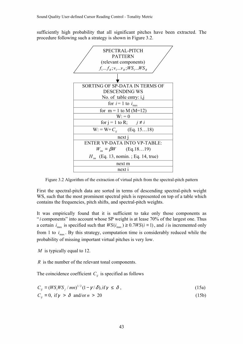
Sound Quality User-defined Cursor Reading Control - Tonality Metric
sufficiently high probability that all significant pitches have been extracted. The procedure following such a strategy is shown in Figure 3.2.
SPECTRAL-PITCH PATTERN
(relevant components) RRR WSWSvvff ...;...;... 111
SORTING OF SP-DATA IN TERMS OF
DESCENDING WS No. of table entry: i,j
for i = 1 to i max
for m = 1 to M (M=12) W: = 0
for j = 1 to R; ij ≠ W: = W+C (Eq. 15…18) ij
next j ENTER VP-DATA INTO VP-TABLE:
WWim β= (Eq.18…19)
imH (Eq. 13, nomin. ; Eq. 14, true) next m next i
Figure 3.2 Algorithm of the extraction of virtual pitch from the spectral-pitch pattern
First the spectral-pitch data are sorted in terms of descending spectral-pitch weight WS, such that the most prominent spectral pitch is represented on top of a table which contains the frequencies, pitch shifts, and spectral-pitch weights. It was empirically found that it is sufficient to take only those components as “ i components” into account whose SP weight is at lease 70% of the largest one. Thus a certain i is specified such that WS , and i is incremented only from 1 to . By this strategy, computation time is considerably reduced while the probability of missing important virtual pitches is very low.
max
maxi)1(7.0)( max =≥ iWSi
M is typically equal to 12. R is the number of the relevant tonal components.
The coincidence coefficient C is specified as follows ij
),/1()/( 2/1 δγ−= mnWSWSC jiij if ,δγ ≤ (15a)
,0=ijC if δγ > and/or (15b) 20>n
43
Sound Quality User-defined Cursor Reading Control - Tonality Metric
• and are the spectral-pitch weights of the and relevant components respectively;
iWS jWS ith jth
• and are the respective subharmonic numbers. While is set by the
algorithm, must for each coincidence test be determined from the formula m n m
n
),5.0/( += ij fmfIntn (16)
• γ is the coefficient which represents the degree of inharmonicity of the tested component pair.
1)/( −= ji fnfγ (17)
• δ is the width of the coincidence interval which is specified by a constant, 0.08.
The weight W which is assigned to the subharmonic of the ith relevant component is essentially the sum of the coincidence coefficients provided by the tested component pairs:
im mth
∑≠=
=R
ijj
ijim CW1
β (18)
• β is a factor. It is called the “fundamental frequency weight.” It has a low-pass
characteristic specified by
[ 14)800/(1 −+= puH imβ ] (19) The evaluation of virtual pitch leads to the virtual-pitch pattern (VP pattern), which contains a list of frequency, virtual pitch and virtual pitch weight triples. The algorithm described here implies that in an actual listening situation, neither of the two pitch modes is completely suppressed; rather, the whole pitch percept is described as a competition between spectral and virtual pitches. These two types of pitch are extracted from the signal and represented by the spectral-pitch pattern and the virtual-pitch pattern.
44

Sound Quality User-defined Cursor Reading Control - Tonality Metric
Chapter 4 Tonality Model in MATLAB This chapter introduces MATLAB, M-file, shows the Data Flow of Tonality model, explains how the Data Flow is related with the algorithm and the MATLAB program, and finally presents some results from model test. 4.1 What is MATLAB? The name MATLAB stands for matrix laboratory. It is a high-performance language for technical computing. It integrates computation, visualization, and programming in an easy-to-use environment where problems and solutions are expressed in familiar mathematical notation. Typical uses include:
o Math and computation o Algorithm development o Modelling, simulation, and prototyping o Data analysis, exploration, and visualization o Scientific and engineering graphics o Application development, including graphical user interface building
MATLAB is an interactive system whose basic data element is an array that does not require dimensioning. This allows you to solve many technical computing problems, especially those with matrix and vector formulations, in a fraction of the time it would take to write a program in a scalar noninteractive language such as C or Fortran. The name MATLAB stands for matrix laboratory. MATLAB was originally written to provide easy access to matrix software developed by the LINPACK and EISPACK projects. Today, MATLAB uses software developed by the LAPACK and ARPACK projects, which together represent the state-of-the-art in software for matrix computation. MATLAB has evolved over a period of years with input from many users. In university environments, it is the standard instructional tool for introductory and advanced courses in mathematics, engineering, and science. In industry, MATLAB is the tool of choice for high-productivity research, development, and analysis. 4.2 What is M-file MATLAB provides a full programming language that enables you to write a series of MATLAB statements into a file and then execute them with a single command. You write your program in an ordinary text file, giving the file a name of filename.m. The term you use for filename becomes the new command that MATLAB associates with the program. The file extension of .m makes this a MATLAB M-file. There are two kinds of M-files in MATLAB, Script M-files and Function M-files. Script M-files do not accept input arguments or return output arguments, while Function M-files can accept input arguments and return output arguments. Script M-files operate on data in the workspace, and are useful for automating a series of steps you need to perform many times, while in Function M-files, internal variables are
45

Sound Quality User-defined Cursor Reading Control - Tonality Metric
local to the function by default, and Function M-files are useful for extending the MATLAB language for your application. An M-file might contain one main function and zero, one or more sub functions, and the M-file name must be the same as the main function name. [4.1] 4.3 Data Flow of Tonality Model The Data Flow for Tonality model is shown in Figure 4.1. It is based on the pitch-evaluation procedure we presented in Figure 3.1 in Chapter 3 and considered how to implement the algorithm in MATLAB programming language.
46
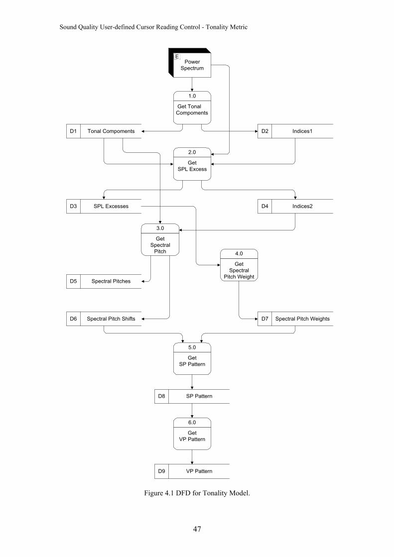
Sound Quality User-defined Cursor Reading Control - Tonality Metric
PowerSpectrum
E
Get TonalCompoments
1.0
D2 Indices1D1 Tonal Compoments
GetSPL Excess
2.0
GetSpectral
Pitch
3.0
GetSpectral
Pitch Weight
4.0
D5 Spectral Pitches
D6 Spectral Pitch Shifts
GetSP Pattern
5.0
D8 SP Pattern
GetVP Pattern
6.0
D9 VP Pattern
D3 SPL Excesses D4 Indices2
D7 Spectral Pitch Weights
Figure 4.1 DFD for Tonality Model.
47
Sound Quality User-defined Cursor Reading Control - Tonality Metric
Power spectrum is the input of the whole model. We get power spectrum from B&K Sound Quality Type 7698 and save it into Excel, then import to MATLAB as a two-column matrix:
Frequency (Hz) SPL (dB) Functions 1.0 – 6.0 are main functions in our MATLAB model. Datastores D1 – D9 are the input or output of the relevant functions, and they are represented in MATLAB as matrices. A matrix is a rectangular array of numbers. Functions 1.0-5.0 are the calculation procedure for Spectral Pitch Pattern. Function 6.0 is for Virtual Pitch Pattern. Function 1.0 implements the procedure of Section 3.2, which extracts the tonal components from power spectrum. Relevant M-file is get_tonal_comp.m in Appendix A. Function 2.0 implements the procedure of Section 3.3.1, which calculate the sound-pressure level excess. Relevant M-file is get_spl_excess.m in Appendix A. Function 3.0 implements the procedure of Section 3.3.2. It calculates the true spectral pitch by evaluating the spectral pitch shift of each relevant tonal component, whose sound-pressure level excess is larger than zero. The relevant M-file is get_spectrum_pitch.m in Appendix A. Function 4.0 implements the procedure of Section 3.4, which calculates the weighting of components whose sound-pressure level excess is larger than zero. The relevant M- file is get_sp_weight.m in Appendix A. Function 5.0 combines all the necessary information for Spectral Pitch Pattern. The relevant M-file is get_SP_Pattern.m in Appendix A. Function 6.0 is related to Section 3.5, which evaluates the true virtual pitch and get Virtual Pitch Pattern. The relevant M-file is get_VP_Pattern.m in Appendix A. D1 contains Tonal Components represented in MATLAB as a two-column matrix:
Frequency (Hz) SPL (dB) D2 (Indices1) is the Power Spectrum row indices used to remember locations of the local maximal samples. Local maximal samples satisfy Eq. (1) and Eq. (2) in Chapter 3. It is represented in MATLAB as a one-column matrix:
Row Indices D3 contains SPL Excesses information represented in MATLAB as a two-column matrix:
Frequency (Hz) SPL Excess (dB)
48
Sound Quality User-defined Cursor Reading Control - Tonality Metric
D4 (Indices2) is the Tonal Components row indices, whose SPL Excess is larger than zero. It is represented in MATLAB as a one-column matrix:
Row Indices Design of D2 and D4 is for remembering the interesting locations for programming purpose. D5 contains Spectral Pitches information represented in MATLAB as a two-column matrix:
Frequency (Hz) Spectral Pitch (pu) D6 contains Spectral Pitch Shifts information represented in MATLAB as a two-column matrix:
Frequency (Hz) Spectral Pitch Shift D7 contains Spectral Pitch Weights information represented in MATLAB as a two-column matrix:
Frequency (Hz) Spectral Pitch Weight D8 contains SP Pattern information represented in MATLAB as a three-column matrix:
Frequency (Hz) Spectral Pitch Shift Spectral Pitch Weight D9 contains VP Pattern information represented in MATLAB as a three-column matrix:
Frequency (Hz) Virtual Pitch (pu) Virtual Pitch Weight 4.4 Model Simplification and Modification The different threshold value of 7 dB in Eq. (2) in Chapter 3 was determined empirically by analysing several complex sounds. But when we test our MATLAB model with some natural speech vowels, we found that the 7 dB is so big that most of the cases, there is no tonal components or very few tonal components can be extracted. But in order to test the other pitch-evaluation procedure we must have some tonal components data. So we change it to 3 dB just for programming and testing purpose. According to the algorithm of virtual pitch evaluation, which is shown in Figure 3. 4 in Chapter 3, we will get a big number of virtual pitches, which is 12 times the number of spectral pitches. But we say that only the five most prominent virtual pitches, which have the higher weight values, are our concern.
49
Sound Quality User-defined Cursor Reading Control - Tonality Metric
4.5 The Relations of Different M-files in Tonality MATLAB Model Functions 1.0-6.0 in Figure 4.1 are implemented as M-files. Each of them has main function and some of them have sub functions. Besides all these main functions and sub functions, we also have some auxiliary functions, which are shared by different main functions or sub functions. Figure 4.2 and Figure 4.3 only show the most related functions in our MATLAB model. Each rectangular means one M-file. The first function name is the main function name, which should be the same as the M-file name. The following function(s) are sub function(s), which are defined in the same M-file. If there is an arrow, from function A to function B, then it means that function A uses function B in its definition. The purpose of presenting functions in this way is to show the layers of different functions. Lev
get_spl_excess
IN
LTH
get_spectrum_pitch
Vu
Specific_LXu
S
z
Figure 4.2 Relations of main, sub and auxiliary functions in different M-files. Figure 4.2 shows the functions and sub functions relationship among four M-files, namely, get_spl_excess.m, get_spectrum_pitch.m, Lev.m and z.m. Function get_spl_excess is the main function to calculate the SPL excesses of tonal components. IN is a sub function to calculate Noise Intensity, present in the critical band around the considered tonal component. LTH is a sub function to calculate the hearing threshold at a certain frequency. Function get_spectrum_pitch is the main function to calculate the spectral pitches for the relevant tonal components whose SPL excess is larger than zero. Vu calculates the induced pitch shifts. Specific_LXu calculates the Specific representations of the SPL excess. Function Lev and z are two
50
Sound Quality User-defined Cursor Reading Control - Tonality Metric
auxiliary functions. They are defined in different M-files. Lev calculates the excitation level, which produced at a certain frequency by one tonal component. S calculates the steepness of the slopes in the excitation level critical-band rate patern. Function S is a sub function in M-file Lev.m. Function z calculates the critical-band rate (Bark) of a certain frequency. Funciton Lev is shared by get_spl_excess and Specific_LXu. Function z is shared by Lev and IN. Get_VP_Pattern
Beta
H
C
Gamma
n
Figure 4.3 Relations of main and sub functions in M-file: get_VP_Pattern.m Figure 4.3 shows the relations of the main function and different sub functions in M-file: get_VP_Pattern.m. Sub function Beta calculates a factor, called the 'fundamental frequency weight'. H calculates the true virtual pitch. C calculates the coincidence coefficient. Gamma calculates the inharmonicity coefficient. Sub function n is related with Eq.16 in Chapter 3. 4.6 A Function M-file Example Let us take M-file: get_tonal_comp.m as an example and see how M-file looks like in MATLAB and how to use it in MATLAB Command window. function [y,z] = Get_tonal_comp(x) %Extraction of tonal components. %Input: power spectrum %Output: tonal components. %Check whether the input matrix validate. [m,n] = size(x); if (~(n == 2) | (m == 1 & n == 1)) error('Input must be a two column vector!') end k = 1; for i = 4:(length(x)-3)
%Look for local maximal samples. if x(i,2)>=x(i+1,2) & x(i,2)>x(i-1,2) & x(i,2)-x(i-3,2)>=3 & x(i,2)-x(i-2,2)>=3 & x(i,2)-x(i+2,2)>=3 & x(i,2)-x(i+3,2)>=3
51
Sound Quality User-defined Cursor Reading Control - Tonality Metric
%Calculate and save the frequency and the SPL values for tonal components.
y(k,1)=x(i,1)+0.46*(x(i+1,2)-x(i-1,2)) y(k,2)=x(i,2)
%Check whether you want to remember the power spectrum indices of the %local maximal samples. if (nargout == 2)
z(k,1)=i end k=k+1;
end end Input x is the power spectrum which contains 401 samples. Output y is the tonal components, and output z is the row indices of the local maximal samples. The if statement:
if x(i,2)>=x(i+1,2) & x(i,2)>x(i-1,2) & x(i,2)-x(i-3,2)>=7 & x(i,2)-x(i-2,2)>=7 & x(i,2)-x(i+2,2)>=7 & x(i,2)-x(i+3,2)>=7
is related to Eq.(1) and Eq.(2) in Chapter 3. The statement: y(k,1)=x(i,1)+0.46*(x(i+1,2)-x(i-1,2)) is related to Eq.(3) in Chapter 3. If we type the following command in MATLAB Command Window,
[tonal_components, indices1] = get_tonal_comp(power_spectrum)
The input: power_spectrum contains the same data as Test 1 in Appendix C. We will get the following results, tonal_components = 1.0e+003 * 0.3879 0.0581 0.7660 0.0332 0.9891 0.0265 1.5282 0.0272 1.8718 0.0397 2.0781 0.0467 2.5091 0.0417 2.6367 0.0439 2.8638 0.0372 3.0911 0.0350 3.3482 0.0406 3.4672 0.0391
52
Sound Quality User-defined Cursor Reading Control - Tonality Metric
3.5950 0.0350 3.8641 0.0268 indices1 = 37 72 93 143 175 194 234 246 267 288 312 323 335 360 The data in variable tonal_components is a list of frequency and SPL values. They will be used in the later SPL Excess and Spectral Pitch calculations, and also being used to generate the plot for Tonal Components. The data in variable indices1 is the row indices of the local maximal samples. The relations between local maximal sample and tonal components can be found in Section 3.2. More information about the other MATLAB functions can be found in Appendix A. 4.7 How to Show the Computational Results? After we have the matrices for power spectrum, tonal components, SPL excesses, spectral pitches pattern and virtual pitch pattern, we want to present them in one figure and list them as different plots. We wrote a Script M-file, namely “show.m” which use MATLAB functions “subplot” and some auxiliary functions defined by us, such as “show_spectrum” and “show_stem”. function show(ps) %show all the figures for the model %show the power spectrum in first plot %'show_spectrum' is a function we defined using Matlab's 'plot' function subplot(5,1,1); show_spectrum(ps) %get tonal components [tc1,idx1]=Get_tonal_comp(ps) %show the tonal components in second plot %'show_stem' is a function we defined using Matlab's 'stem' function, y is between 1 %to 5. subplot(5,1,2); show_stem(tc1) ylabel('SPL(dB)')
53
Sound Quality User-defined Cursor Reading Control - Tonality Metric
%get the SPL excess [tc2,idx2]=Get_spl_excess(ps,tc1,idx1) %show the SPL excess value in third plot subplot(5,1,3); show_stem(tc2) ylabel('SPL EXCESS') %calculate spectral pitch, pitch shift, spectral weight [spec_pitch,pitch_shift]=Get_spectrum_pitch(tc1,idx2) spec_weight=Get_sp_weight(tc2) %show WS in fourth plot subplot(5,1,4); show_stem(spec_weight) ylim([0 1]) ylabel('WS') %calculate virtual pitch vpp_input=Get_SP_Pattern(pitch_shift,spec_weight) vpp_output=Get_VP_Pattern(vpp_input) %show Virtual Pitch weight in fifth plot subplot(5,1,5); stem(vpp_output(:,1)/1000,vpp_output(:,3),'fill') xlim([0 5]) xlabel('Frequency(KHz)') ylabel('WP') The auxiliary function show_spectrum.m is as follows. function show_spectrum(x) % show spectrum plot(x(:,1)/1000,x(:,2)) ylabel('SPL(dB)') xlim([0 5]) The auxiliary function show_stem.m is as follows. function show_stem(x) % show stem stem(x(:,1)/1000,x(:,2),'fill') xlim([0 5])
54
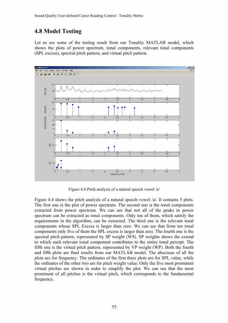
Sound Quality User-defined Cursor Reading Control - Tonality Metric
4.8 Model Testing Let us see some of the testing result from our Tonality MATLAB model, which shows the plots of power spectrum, tonal components, relevant tonal components (SPL excess), spectral pitch pattern, and virtual pitch pattern.
Figure 4.4 Pitch analysis of a natural speech vowel /a/ Figure 4.4 shows the pitch analysis of a natural speech vowel /a/. It contains 5 plots. The first one is the plot of power spectrum. The second one is the tonal components extracted from power spectrum. We can see that not all of the peaks in power spectrum can be extracted as tonal components. Only ten of them, which satisfy the requirements in the algorithm, can be extracted. The third one is the relevant tonal components whose SPL Excess is larger than zero. We can see that from ten tonal components only five of them the SPL excess is larger than zero. The fourth one is the spectral pitch pattern, represented by SP weight (WS). SP weights shows the extend to which each relevant tonal component contributes to the entire tonal percept. The fifth one is the virtual pitch pattern, represented by VP weight (WP). Both the fourth and fifth plots are final results from our MATLAB model. The abscissas of all the plots are for frequency. The ordinates of the first three plots are for SPL value, while the ordinates of the other two are for pitch weight value. Only the five most prominent virtual pitches are shown in order to simplify the plot. We can see that the most prominent of all pitches is the virtual pitch, which corresponds to the fundamental frequency.
55
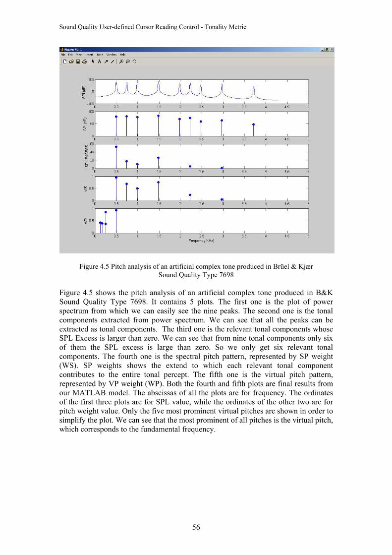
Sound Quality User-defined Cursor Reading Control - Tonality Metric
Figure 4.5 Pitch analysis of an artificial complex tone produced in Brüel & Kjær Sound Quality Type 7698
Figure 4.5 shows the pitch analysis of an artificial complex tone produced in B&K Sound Quality Type 7698. It contains 5 plots. The first one is the plot of power spectrum from which we can easily see the nine peaks. The second one is the tonal components extracted from power spectrum. We can see that all the peaks can be extracted as tonal components. The third one is the relevant tonal components whose SPL Excess is larger than zero. We can see that from nine tonal components only six of them the SPL excess is large than zero. So we only get six relevant tonal components. The fourth one is the spectral pitch pattern, represented by SP weight (WS). SP weights shows the extend to which each relevant tonal component contributes to the entire tonal percept. The fifth one is the virtual pitch pattern, represented by VP weight (WP). Both the fourth and fifth plots are final results from our MATLAB model. The abscissas of all the plots are for frequency. The ordinates of the first three plots are for SPL value, while the ordinates of the other two are for pitch weight value. Only the five most prominent virtual pitches are shown in order to simplify the plot. We can see that the most prominent of all pitches is the virtual pitch, which corresponds to the fundamental frequency.
56
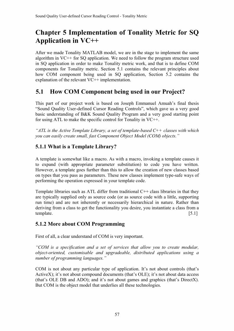
Sound Quality User-defined Cursor Reading Control - Tonality Metric
Chapter 5 Implementation of Tonality Metric for SQ Application in VC++ After we made Tonality MATLAB model, we are in the stage to implement the same algorithm in VC++ for SQ application. We need to follow the program structure used in SQ application in order to make Tonality metric work, and that is to define COM components for Tonality metric. Section 5.1 contains the relevant principles about how COM component being used in SQ application, Section 5.2 contains the explanation of the relevant VC++ implementation. 5.1 How COM Component being used in our Project? This part of our project work is based on Joseph Emmanuel Amuah’s final thesis “Sound Quality User-defined Cursor Reading Controls”, which gave us a very good basic understanding of B&K Sound Quality Program and a very good starting point for using ATL to make the specific control for Tonality in VC++. “ATL is the Active Template Library, a set of template-based C++ classes with which you can easily create small, fast Component Object Model (COM) objects.”
5.1.1 What is a Template Library? A template is somewhat like a macro. As with a macro, invoking a template causes it to expand (with appropriate parameter substitution) to code you have written. However, a template goes further than this to allow the creation of new classes based on types that you pass as parameters. These new classes implement type-safe ways of performing the operation expressed in your template code. Template libraries such as ATL differ from traditional C++ class libraries in that they are typically supplied only as source code (or as source code with a little, supporting run time) and are not inherently or necessarily hierarchical in nature. Rather than deriving from a class to get the functionality you desire, you instantiate a class from a template. [5.1]
5.1.2 More about COM Programming First of all, a clear understand of COM is very important. “COM is a specification and a set of services that allow you to create modular, object-oriented, customisable and upgradeable, distributed applications using a number of programming languages.”
COM is not about any particular type of application. It’s not about controls (that’s ActiveX); it’s not about compound documents (that’s OLE); it’s not about data access (that’s OLE DB and ADO); and it’s not about games and graphics (that’s DirectX). But COM is the object model that underlies all these technologies.
57
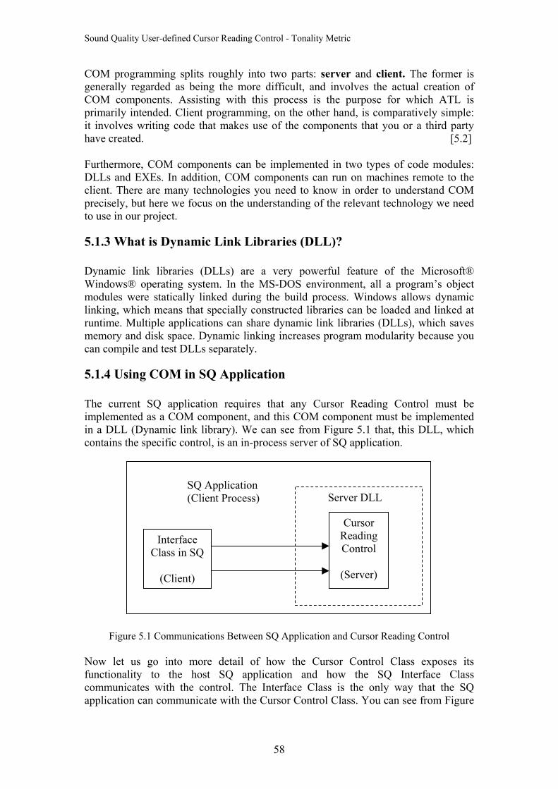
Sound Quality User-defined Cursor Reading Control - Tonality Metric
COM programming splits roughly into two parts: server and client. The former is generally regarded as being the more difficult, and involves the actual creation of COM components. Assisting with this process is the purpose for which ATL is primarily intended. Client programming, on the other hand, is comparatively simple: it involves writing code that makes use of the components that you or a third party have created. [5.2] Furthermore, COM components can be implemented in two types of code modules: DLLs and EXEs. In addition, COM components can run on machines remote to the client. There are many technologies you need to know in order to understand COM precisely, but here we focus on the understanding of the relevant technology we need to use in our project.
5.1.3 What is Dynamic Link Libraries (DLL)? Dynamic link libraries (DLLs) are a very powerful feature of the Microsoft® Windows® operating system. In the MS-DOS environment, all a program’s object modules were statically linked during the build process. Windows allows dynamic linking, which means that specially constructed libraries can be loaded and linked at runtime. Multiple applications can share dynamic link libraries (DLLs), which saves memory and disk space. Dynamic linking increases program modularity because you can compile and test DLLs separately.
5.1.4 Using COM in SQ Application The current SQ application requires that any Cursor Reading Control must be implemented as a COM component, and this COM component must be implemented in a DLL (Dynamic link library). We can see from Figure 5.1 that, this DLL, which contains the specific control, is an in-process server of SQ application.
SQ Application (Client Process)
Interface Class in SQ
(Client)
Server DLL
Cursor Reading Control
(Server)
Figure 5.1 Communications Between SQ Application and Cursor Reading Control Now let us go into more detail of how the Cursor Control Class exposes its functionality to the host SQ application and how the SQ Interface Class communicates with the control. The Interface Class is the only way that the SQ application can communicate with the Cursor Control Class. You can see from Figure
58
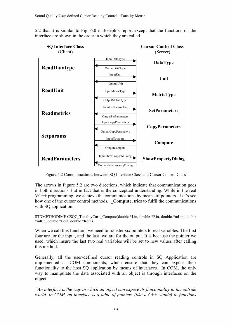
Sound Quality User-defined Cursor Reading Control - Tonality Metric
5.2 that it is similar to Fig. 6.0 in Joseph’s report except that the functions on the interface are shown in the order in which they are called. SQ Interface Class Cursor Control Class (Client) (Server)
_
_C
_Sho
InputShowPropertyDialog
OutputShowpropertyDialog
InputCompute
OutputCompute
InputCopyParameters
OutputCopyParameters
InputSetParameters
OutputSetParameters
InputDataType
OutputDataType
InputUnit
OutputUnit
InputMetricType
OutputMetricType
Thin VChowi ST*m Wfouusthi Geimfunwaob “Awo
ReadDatatype
ReadUnit
Readmetrics
Setparams
ReadParameters
Figure 5.2 Communications between SQ Interface Class and
e arrows in Figure 5.2 are two directions, which indicate both directions, but in fact that is the conceptual understa++ programming, we achieve the communications by mea
w one of the cursor control methods, _Compute, tries to fth SQ application.
DMETHODIMP CSQC_TonalityCur::_Compute(double *Lin, doubleRin, double *Lout, double *Rout)
hen we call this function, we need to transfer six pointers tr are for the input, and the last two are for the output. It i
ed, which insure the last two real variables will be set tos method.
nerally, all the user-defined cursor reading controls plemented as COM components, which ensure that ctionality to the host SQ application by means of interfay to manipulate the data associated with an object is thject.
n interface is the way in which an object can expose its furld. In COM, an interface is a table of pointers (like a C
59
_DataType
_Unit
_MetricType
SetParameters
opyParameters
_Compute
wPropertyDialog
Cursor Control Class
that communication goes nding. While in the real ns of pointers. Let’s see ulfil the communications
*Rin, double *mLin, double
o real variables. The first s because the pointer we new values after calling
in SQ Application are they can expose their ces. In COM, the only rough interfaces on the
nctionality to the outside ++ vtable) to functions
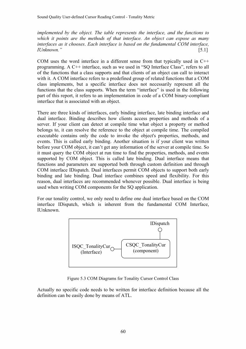
Sound Quality User-defined Cursor Reading Control - Tonality Metric
implemented by the object. The table represents the interface, and the functions to which it points are the methods of that interface. An object can expose as many interfaces as it chooses. Each interface is based on the fundamental COM interface, IUnknown.” [5.1] COM uses the word interface in a different sense from that typically used in C++ programming. A C++ interface, such as we used in “SQ Interface Class”, refers to all of the functions that a class supports and that clients of an object can call to interact with it. A COM interface refers to a predefined group of related functions that a COM class implements, but a specific interface does not necessarily represent all the functions that the class supports. When the term “interface” is used in the following part of this report, it refers to an implementation in code of a COM binary-compliant interface that is associated with an object. There are three kinds of interfaces, early binding interface, late binding interface and dual interface. Binding describes how clients access properties and methods of a server. If your client can detect at compile time what object a property or method belongs to, it can resolve the reference to the object at compile time. The compiled executable contains only the code to invoke the object's properties, methods, and events. This is called early binding. Another situation is if your client was written before your COM object, it can’t get any information of the server at compile time. So it must query the COM object at run time to find the properties, methods, and events supported by COM object. This is called late binding. Dual interface means that functions and parameters are supported both through custom definition and through COM interface IDispatch. Dual interfaces permit COM objects to support both early binding and late binding. Dual interface combines speed and flexibility. For this reason, dual interfaces are recommended whenever possible. Dual interface is being used when writing COM components for the SQ application. For our tonality control, we only need to define one dual interface based on the COM interface IDispatch, which is inherent from the fundamental COM Interface, IUnknown.
IDispatch ISQC_TonalityCur (Interface)
CSQC_TonalityCur(component)
Figure 5.3 COM Diagrams for Tonality Cursor Control Class
Actually no specific code needs to be written for interface definition because all the definition can be easily done by means of ATL.
60
Sound Quality User-defined Cursor Reading Control - Tonality Metric
5.1.5 More about COM Interface In the following part of this section, we will first introduce the notions, Interface Definition and Interface Implementation. Second we will discuss the difference between these two concepts. Last we will introduce The Interface Definition Language (IDL), which is used to write interface definition, and furthermore we present the concept of type library, which is best thought of as a binary version of an Interface Definition Language (IDL) file. • Interface Definition and Interface Implementation COM makes a fundamental distinction between interface definitions and their implementations. An interface is actually a contract that consists of a group of related function prototypes whose usage is defined but whose implementation is not. These function prototypes are equivalent to pure virtual base classes in C++ programming. An interface definition specifies the interface's member functions, called methods, their return types, the number and types of their parameters, and what they must do. There is no implementation associated with an interface. [5.1] An interface implementation is the code a programmer supplies to carry out the actions specified in an interface definition. Implementations of many of the interfaces a programmer can use in an object-based application are included in the COM libraries. However, programmers are free to ignore these implementations and write their own. An interface implementation is to be associated with an object when an instance of that object is created, and the implementation provides the services that the object offers. [5.1] The interface definition would not specify how the functions are to be implemented in code. In implementing the interface, different programmers might implement it in different ways such as using different data structures and different data flows and control flows. Regardless of a particular implementation of the interface methods, the in-memory representation of a pointer to an interface, and therefore its use by a client, is completely determined by the interface definition. • How to Understand Interface Simple objects support only a single interface. More complicated objects, such as embeddable objects, typically support several interfaces. Clients have access to a COM object only through a pointer to one of its interfaces, which, in turn, allows the client to call any of the methods that make up that interface. These methods determine how a client can use the object's data. [5.1] Interfaces define a contract between an object and its clients. The contract specifies the methods that must be associated with each interface and what the behaviour of each of the methods must be in terms of input and output. The contract generally does not define how to implement the methods in an interface. Another important aspect of the contract is that if an object supports an interface, it must support all of that interface's methods in some way. Not all of the methods in an implementation need to do something—if an object does not support the function implied by a method, its
61
Sound Quality User-defined Cursor Reading Control - Tonality Metric
implementation may be a simple return or perhaps the return of a meaningful error message—but the methods must exist. [5.1] • The Interface Definition Language Although ATL makes COM programming more simple in a way that you do not need to define the interfaces by your own code. Instead, you just follow some instructions and set-up some dialogs, then ATL will help you generate the code for interface definition. But understanding of how an unambiguous definition of the interfaces is implemented will be very helpful for you to understand the technology behind ATL COM programming. Interface definition is achieved by means of The Interface Definition Language (IDL). The Interface Definition Language (IDL) is used to provide complete definitions of COM interfaces, and it allows us to associate the methods of an interface with its IID (Interface Identifier), to specify details of the interface in a form that can be machine-processed to produce marshalling code, and to instruct clients and servers on how they should allocate and deallocate memory. [5.2] • Type Library COM is a binary standard for component implementation and integration, and therefore the language used to build or call COM objects is irrelevant. Since our component is already built on COM, you might wonder why anything special is required to make it accessible to developers using other languages. Well, to make a component more accessible to developers working in other languages, you need to create a type library. [5.1] A type library is best thought of as a binary (or compiled) version of an Interface Definition Language (IDL) file. It contains a binary description of the interfaces exposed by a component, defining the methods along with their parameters and return types. Many environments support type libraries: Visual Basic, Visual J++, and Microsoft Visual C++® all understand type libraries; so do Delphi, Microsoft Visual FoxPro®, and Microsoft Transaction Server. Rumor says that the next version of Microsoft (Visual) Macro Assembler will support COM via type libraries. [5.1] 5.2 Tonality Implementation in VC++ Before starting to write VC++ code, there are several things that we need to consider. One is what kinds of Data Structures should be used to store the data that we manipulate in each steps of the algorithm; the second is the data flow of our program based on the data structure we use. The first problem is solved by using the Vector Container Type, which is part of C++ Standard Template Library (STL), and the second problem is solved by using the analysis of our previous work, please refer to Figure 4.1 DFD for Tonality Model. In the following part of this section, we will highlight some special points, which proved to be very helpful for making the Tonality Control in VC++.
62
Sound Quality User-defined Cursor Reading Control - Tonality Metric
5.2.1 Why Choose Vector Container Type? For the purposes of making Tonality Control, We firstly think about using Array. In C++, An array is a collection of objects of a single data type. Each element is accessed by its position in the array, which is called indexing or subscripting. If the number of elements to be stored is known at compile time, an array can be used. Apparently this is not suitable for our purpose, because in each procedure the result of the calculation is generated dynamically, the number of elements to be stored is unknown and likely to vary widely. So using dynamically allocated storage for each object turns out to be a better way, and sequence container types are considered. A sequence container holds an ordered collection of elements of a single type. The sequence container types in VC++ includes, the vector, the deque, and the list, which all grow dynamically. The vector class provides an alternative representation to the built-in array, and its usage is highly recommended by experienced programmers. The vector class is part of the standard library introduced with Standard C++. There are two very different forms of using a vector, the array idiom and the STL idiom. The array idiom is analogous to defining a built-in array. In the STL idiom, a vector is used very differently. Rather than define it with a given size, we define an empty vector. Rather than using index and assign to an element, we instead insert an element into the vector. There are some STL functions in Visual C++ that we can use to operate the vector. The following list contains some of them, which are frequently used in our code. • vector::begin - Returns an iterator to start traversal of the vector. • vector::end - Returns an iterator for the last element of the vector. • vector::push_back - Appends (inserts) an element to the end of a vector, allocating
memory for it if necessary. • vector::iterator - Traverses the vector. An iterator is a standard library class that
represents the functionality of a pointer. One can dereference the iterator and access the actual object addressed.
• vector::size - Returns number of elements in the vector. • vector::erase - Deletes elements from a vector (single & range). The second form of vector, the STL idiom, is chosen due to the dynamic nature of the problem. Let’s see an example about how to define power spectrum as a vector type in C++ code. The considerations are, power spectrum of a signal can be presented as a list of frequency and SPL pairs. In C++, the pair class is part of the standard library, and allows us to associate two values of either the same or different types within a single object. So this is defined in, POWER_SPECTRUM_ITEM, which contains the pair of two double values. In fact these two double values refer to frequency and SPL respectively. Then we define a vector type, POWER_SPECTRUM, which contains POWER_SPECTRUM_ITEM. The code is as follows, #include <vector> using namespace std ; typedef struct pair<double, double> POWER_SPECTRUM_ITEM ; typedef vector<POWER_SPECTRUM_ITEM> POWER_SPECTRUM;
63
Sound Quality User-defined Cursor Reading Control - Tonality Metric
We have also defined some other vector types, such as SPECTRUM_PITCH, SPECTRUM_PITCH_SHIFT, SPECTRUM_PITCH_WEIGHT, SP_PATTERN, VP_PATTERN. For more information about the other vector type definitions, please refer to the header file, SQC_TonalityCur.h in Appendix B. Especially, we want to mention the definition of the following vector for the purpose of remembering the indices as shown in Figure 4.1. typedef vector<POWER_SPECTRUM::iterator> INDICES; We define the INDICES as a vector type contains the iterator of POWER_SPECTRUM. So actually INDICES is a vector type contains pointers, which can be used to dereference and access the actual object addressed.
5.2.2 Using Pointers Dynamic memory allocation and pointer manipulation is a fundamental aspect of real-world programming in C++. It is very efficient to transfer the pointer to a vector instead of the whole vector when you call some sub functions from the main function because it provides a way that can avoid transferring the whole variable, but only a pointer to that variable instead. It becomes more efficient when the variable needs big storage space. Let’s look at an example of the Get_Tonal_Comp function. This procedure is used after we call Get_Power_Spectrum. We need to transfer three pointers as parameters, which are referred to three real variables. After calling this function, the real variables’ value is changed because the pointers we use in this function definition. The first variable to this function call is the input, while the other two variables are the output because we assigned new values to them. Void CSQC_TonalityCur::Calc::Get_Tonal_Comp (POWER_SPECTRUM *pPS, POWER_SPECTRUM *pTC, INDICES *p_idcs1) { POWER_SPECTRUM::iterator i; POWER_SPECTRUM_ITEM tc_item; for( i = pPS->begin()+3; i != pPS->end()-3 ; i++) {
if ((*i).second >= (*(i+1)).second && (*i).second > (*(i-1)).second && (*i).second – (*(i-3)).second >=3 && (*i).second - (*(i-2)).second >= 3 && (*i).second – (*(i+2)).second >=3 && (*i).second - (*(i+3)).second >= 3)
{ tc_item.first = (*i).first+0.46 * ((*(i+1)).second - (*(i-1)).second); tc_item.second =(*i).second; pTC->push_back(tc_item); p_idcs1->push_back(i); } } } More explanation should be given for the last two lines in for loop. The first line pTC->push_back(tc_item) means to save the result into the vector by means of push_back method which is provided by the vector container type in Standard Type
64
Sound Quality User-defined Cursor Reading Control - Tonality Metric
Library(STL) in Visual C++. The second line p_idcs1->push_back(i) means to save the iterator of the current items which you just saved. An iterator can also be understood as a pointer to the current element or item in the vector in our usage. While precisely speaking, an iterator provides a general method of successively accessing each element within any of the sequential or associative container types. For more information about iterator of vector container types, STL or pointers, please refer to reference [5.3]. On the other hand, using pointers might cause some problems in some situations. For example, if you have a variable, which needs a large space to store the relevant information, and more than two pointers refer to it in your application. Let us assume a situation as follows: you have such two procedures in your main program, which use these two pointers respectively. Then what happened when both of the procedures trying to access the same variable? Yes, it will cause some security problems--make the data in the variable unsafe. So how can we solve it and avoid this kind of security problems? Actually the ultimate problem of this question is also one of the most critical issues of the design of libraries and long running programs, that is memory management. A library writer doesn’t in general know if a library will be part of an application where memory is scarce, where a memory leak would be a serious problem, or where memory-management overhead could be a serious liability. The fundamental question about memory management can be stated in this way: If f() passes or returns a pointer to an object to g(), who is responsible for the object’s destruction? A secondary question must also be answered: When can it be safely destroyed? In particular, these questions are critical to designers and users of container classes, such as lists, arrays, and associative arrays. From the point of view of a library provider, the ideal answers are “the system” and “whenever nobody is using the object any longer.” A system doing this is usually said to be garbage collecting, and the part of the system that determines that nobody uses a given object and destroys it is called the garbage collector. [5.4] Unfortunately, garbage collection implies overheads in runtime and space, service interruptions, special supportive hardware, trouble with linking to program fragments written in other languages, or system complexity. This, many users cannot afford. Consequently, although garbage collecting implementations of C++ exist, most C++ programs cannot rely on garbage collection and must devise strategies for managing objects on the free store without help from the system. [5.4] Garbage Collection can be seen as a way of simulating an infinite memory in a limited memory. For more information about Garbage Collection, please refer to [5.3] and [5.4]. This kind of security problem can be solved in C++ programming by using Exception Handling in both procedures to protect the same variable, in each procedure, use dynamic memory allocation and deallocation for the pointer. Exception handling is a mechanism that allows two separately developed program components to communicate when a program anomaly, called an exception, is encountered during the execution of the program. It is similar idea as critical region in Concurrent
65
Sound Quality User-defined Cursor Reading Control - Tonality Metric
Programming. Exception handling provides a way of transferring control and information from a point in the execution of a program to an exception handler associated with a point previously passed by the execution. A handler will be invoked only by a throw-expression invoked in code executed in the handler’s try-block or in functions called from the handler’s try-block. For more information about exception handler, throw-expression and try-block, please refer to [5.4]. Dynamic memory allocation and deallocation in C++ means that objects are allocated by a run-time library, which invoked during program execution. Contrariwise, for static memory allocation, the objects are allocated by the compiler as it processes the program source code. Whenever using the dynamic memory allocation, one needs to remember to delete the dynamically allocated memory. Otherwise it ends up with a memory leak. A memory leak is a chunk of dynamically allocated memory that we no longer have a pointer to, and thus we cannot return it to the operating system for later reuse. Actually, we simply solve this security problem in our C++ program by making sure that no pointers access the same variable at the same time. We think it is the easiest and the most convenient way to solve the problem and we do not need to bother too much about the usage of Exception Handling, which is a little bit complicated for us to try when we have strict project time limitation.
5.2.3 Using The Generic Algorithms In the VP Pattern calculation procedure in Tonality algorithm, we need to sort the SP Pattern in terms of descending WS (Spectrum Weight). Many sorting algorithms exist, such as Bubble Sort, Heap Sort, Insertion Sort, Merge Sort, Quick Sort and so on. But the most efficient way to solve this problem is not to write our own algorithm, but to use the Generic Algorithms in VC++. Generic Algorithm is also part of Standard Template Library (STL). To find the minimum or maximum value among the elements of a vector, we must instead invoke one of the generic algorithms: “algorithms” because they implement common operations such as min(), max(), find(), and sort(); “generic” because they operate across multiple container types—not only the vector and list types, for example, but also the built-in array type. The container is bound to the generic algorithm operating on it by an iterator pair marking the elements to traverse. [5.3] Each generic algorithm is implemented independently of the individual container types. Because the type dependence of the algorithm has been removed, a single template instance can work across all the container types as well as the built-in array type. [5.3] For more information about the mechanism of Generic Algorithms, Please refer to reference [5.3] and [5.1]. Let’s look at an example from my VC++ code to show how we use it when we need to solve our specific problem. The structure and type definition defined in the header file. struct VP_PATTERN_ITEM { double frequency; double vp_pitch;
66
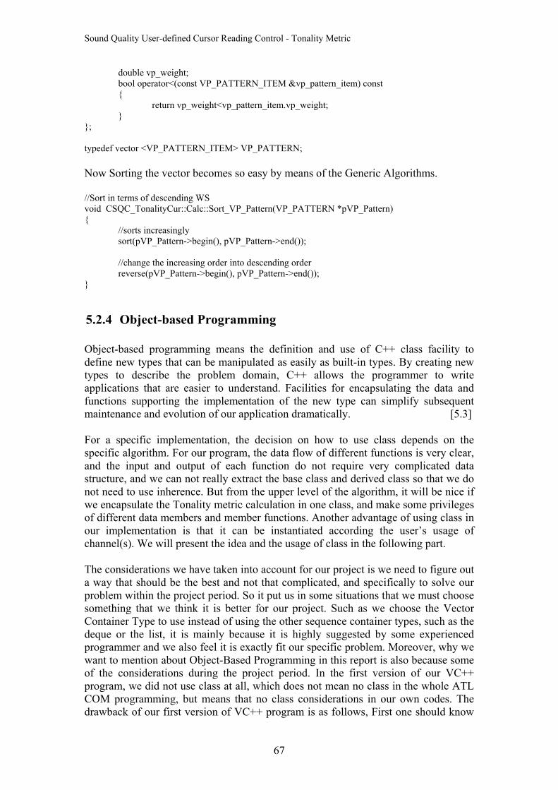
Sound Quality User-defined Cursor Reading Control - Tonality Metric
double vp_weight; bool operator<(const VP_PATTERN_ITEM &vp_pattern_item) const { return vp_weight<vp_pattern_item.vp_weight; } }; typedef vector <VP_PATTERN_ITEM> VP_PATTERN; Now Sorting the vector becomes so easy by means of the Generic Algorithms. //Sort in terms of descending WS void CSQC_TonalityCur::Calc::Sort_VP_Pattern(VP_PATTERN *pVP_Pattern) { //sorts increasingly
sort(pVP_Pattern->begin(), pVP_Pattern->end()); //change the increasing order into descending order reverse(pVP_Pattern->begin(), pVP_Pattern->end());
}
5.2.4 Object-based Programming Object-based programming means the definition and use of C++ class facility to define new types that can be manipulated as easily as built-in types. By creating new types to describe the problem domain, C++ allows the programmer to write applications that are easier to understand. Facilities for encapsulating the data and functions supporting the implementation of the new type can simplify subsequent maintenance and evolution of our application dramatically. [5.3] For a specific implementation, the decision on how to use class depends on the specific algorithm. For our program, the data flow of different functions is very clear, and the input and output of each function do not require very complicated data structure, and we can not really extract the base class and derived class so that we do not need to use inherence. But from the upper level of the algorithm, it will be nice if we encapsulate the Tonality metric calculation in one class, and make some privileges of different data members and member functions. Another advantage of using class in our implementation is that it can be instantiated according the user’s usage of channel(s). We will present the idea and the usage of class in the following part. The considerations we have taken into account for our project is we need to figure out a way that should be the best and not that complicated, and specifically to solve our problem within the project period. So it put us in some situations that we must choose something that we think it is better for our project. Such as we choose the Vector Container Type to use instead of using the other sequence container types, such as the deque or the list, it is mainly because it is highly suggested by some experienced programmer and we also feel it is exactly fit our specific problem. Moreover, why we want to mention about Object-Based Programming in this report is also because some of the considerations during the project period. In the first version of our VC++ program, we did not use class at all, which does not mean no class in the whole ATL COM programming, but means that no class considerations in our own codes. The drawback of our first version of VC++ program is as follows, First one should know
67
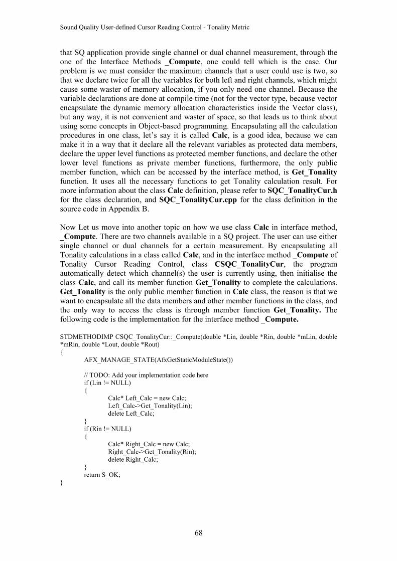
Sound Quality User-defined Cursor Reading Control - Tonality Metric
that SQ application provide single channel or dual channel measurement, through the one of the Interface Methods _Compute, one could tell which is the case. Our problem is we must consider the maximum channels that a user could use is two, so that we declare twice for all the variables for both left and right channels, which might cause some waster of memory allocation, if you only need one channel. Because the variable declarations are done at compile time (not for the vector type, because vector encapsulate the dynamic memory allocation characteristics inside the Vector class), but any way, it is not convenient and waster of space, so that leads us to think about using some concepts in Object-based programming. Encapsulating all the calculation procedures in one class, let’s say it is called Calc, is a good idea, because we can make it in a way that it declare all the relevant variables as protected data members, declare the upper level functions as protected member functions, and declare the other lower level functions as private member functions, furthermore, the only public member function, which can be accessed by the interface method, is Get_Tonality function. It uses all the necessary functions to get Tonality calculation result. For more information about the class Calc definition, please refer to SQC_TonalityCur.h for the class declaration, and SQC_TonalityCur.cpp for the class definition in the source code in Appendix B. Now Let us move into another topic on how we use class Calc in interface method, _Compute. There are two channels available in a SQ project. The user can use either single channel or dual channels for a certain measurement. By encapsulating all Tonality calculations in a class called Calc, and in the interface method _Compute of Tonality Cursor Reading Control, class CSQC_TonalityCur, the program automatically detect which channel(s) the user is currently using, then initialise the class Calc, and call its member function Get_Tonality to complete the calculations. Get_Tonality is the only public member function in Calc class, the reason is that we want to encapsulate all the data members and other member functions in the class, and the only way to access the class is through member function Get_Tonality. The following code is the implementation for the interface method _Compute. STDMETHODIMP CSQC_TonalityCur::_Compute(double *Lin, double *Rin, double *mLin, double *mRin, double *Lout, double *Rout) { AFX_MANAGE_STATE(AfxGetStaticModuleState()) // TODO: Add your implementation code here if (Lin != NULL) { Calc* Left_Calc = new Calc; Left_Calc->Get_Tonality(Lin); delete Left_Calc; } if (Rin != NULL) { Calc* Right_Calc = new Calc; Right_Calc->Get_Tonality(Rin); delete Right_Calc; } return S_OK; }
68

Sound Quality User-defined Cursor Reading Control - Tonality Metric
For more information about class CSQC_TonalityCur, Please refer to the header file SQC_TonalityCur.h and the definition of the class in file SQC_TonalityCur.cpp in Appendix B.
69
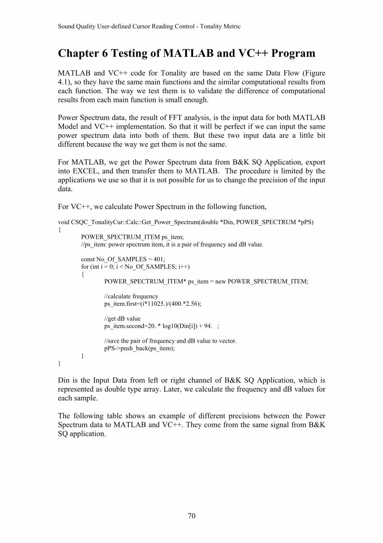
Sound Quality User-defined Cursor Reading Control - Tonality Metric
Chapter 6 Testing of MATLAB and VC++ Program MATLAB and VC++ code for Tonality are based on the same Data Flow (Figure 4.1), so they have the same main functions and the similar computational results from each function. The way we test them is to validate the difference of computational results from each main function is small enough. Power Spectrum data, the result of FFT analysis, is the input data for both MATLAB Model and VC++ implementation. So that it will be perfect if we can input the same power spectrum data into both of them. But these two input data are a little bit different because the way we get them is not the same. For MATLAB, we get the Power Spectrum data from B&K SQ Application, export into EXCEL, and then transfer them to MATLAB. The procedure is limited by the applications we use so that it is not possible for us to change the precision of the input data. For VC++, we calculate Power Spectrum in the following function, void CSQC_TonalityCur::Calc::Get_Power_Spectrum(double *Din, POWER_SPECTRUM *pPS) {
POWER_SPECTRUM_ITEM ps_item; //ps_item: power spectrum item, it is a pair of frequency and dB value.
const No_Of_SAMPLES = 401; for (int i = 0; i < No_Of_SAMPLES; i++) {
POWER_SPECTRUM_ITEM* ps_item = new POWER_SPECTRUM_ITEM; //calculate frequency
ps_item.first=(i*11025.)/(400.*2.56);
//get dB value ps_item.second=20. * log10(Din[i]) + 94. ;
//save the pair of frequency and dB value to vector.
pPS->push_back(ps_item); } } Din is the Input Data from left or right channel of B&K SQ Application, which is represented as double type array. Later, we calculate the frequency and dB values for each sample. The following table shows an example of different precisions between the Power Spectrum data to MATLAB and VC++. They come from the same signal from B&K SQ application.
70
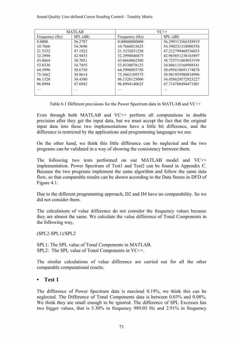
Sound Quality User-defined Cursor Reading Control - Tonality Metric
MATLAB VC++ Frequency (Hz) SPL (dB) Frequency (Hz) SPL (dB) 0.0000 10.7666 21.5332 32.2998 43.0664 53.8330 64.5996 75.3662 86.1328 96.8994 …
56.2787 54.3696 47.1922 42.9453 38.7051 34.7855 30.6750 30.9614 34.4380 47.6942 …
0.00000000000 10.7666015625 21.5332031250 32.2998046875 43.0664062500 53.8330078125 64.5996093750 75.3662109375 86.1328125000 96.8994140625 …
56.299313566358919 54.390231318086556 47.212799468536033 42.965851238165897 38.725731869053199 34.806115168988541 30.695610691174878 30.981955980834996 34.458624572923227 47.714788494471001 …
Table 6.1 Different precisions for the Power Spectrum data in MATLAB and VC++
Even through both MATLAB and VC++ perform all computations in double precision after they get the input data, but we must accept the fact that the original input data into these two implementations have a little bit difference, and the difference is restricted by the applications and programming languages we use. On the other hand, we think this little difference can be neglected and the two programs can be validated in a way of showing the consistency between them. The following two tests performed on our MATLAB model and VC++ implementation. Power Spectrum of Test1 and Test2 can be found in Appendix C. Because the two programs implement the same algorithm and follow the same data flow, so that comparable results can be shown according to the Data Stores in DFD of Figure 4.1. Due to the different programming approach, D2 and D4 have no comparability. So we did not consider them. The calculations of value difference do not consider the frequency values because they are almost the same. We calculate the value difference of Tonal Components in the following way, (SPL2-SPL1)/SPL2 SPL1: The SPL value of Tonal Components in MATLAB. SPL2: The SPL value of Tonal Components in VC++. The similar calculations of value difference are carried out for all the other comparable computational results. • Test 1 The difference of Power Spectrum data is maximal 0.19%, we think this can be neglected. The Difference of Tonal Components data is between 0.03% and 0.08%. We think they are small enough to be ignored. The difference of SPL Excesses has two bigger values, that is 5.30% in frequency 989.05 Hz and 2.91% in frequency
71
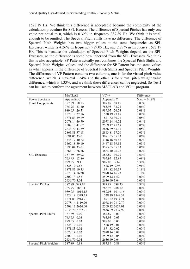
Sound Quality User-defined Cursor Reading Control - Tonality Metric
1528.19 Hz. We think this difference is acceptable because the complexity of the calculation procedure for SPL Excess. The difference of Spectral Pitches has only one value not equal to 0, which is 0.32% in frequency 387.89 Hz. We think it is small enough to be omitted. The Spectral Pitch Shifts have no difference. The difference of Spectral Pitch Weights has two bigger values at the same frequencies as SPL Excesses, which is 4.26% in frequency 989.05 Hz, and 2.27% in frequency 1528.19 Hz. This is because the calculation of Spectral Pitch Weights depend on the SPL Excesses, so the difference is some how inherited from the SPL Excesses. We think this is also acceptable. SP Pattern actually just combines the Spectral Pitch Shifts and Spectral Pitch Weights values, and the difference for SP Pattern has the same values as what appears in the difference of Spectral Pitch Shifts and Spectral Pitch Weights. The difference of VP Pattern contains two columns, one is for the virtual pitch value difference, which is maximal 0.34% and the other is for virtual pitch weight value difference, which is 1.33%, and we think these differences can be neglected. So Test1 can be used to conform the agreement between MATLAB and VC++ program. MATLAB VC++ Difference Power Spectrum Appendix C Appendix C Max. = 0.19% Tonal Components
387.89 58.13 765.95 33.20 989.05 26.51 1528.19 27.16 1871.83 39.69 2078.14 46.70 2509.13 41.67 2636.70 43.89 2863.81 37.18 3091.05 35.01 3348.17 40.62 3467.18 39.10 3595.04 35.01 3864.10 26.76
387.89 58.15 765.95 33.22 989.05 26.53 1528.19 27.18 1871.82 39.71 2078.14 46.72 2509.12 41.69 2636.69 43.91 2863.81 37.20 3091.05 35.03 3348.18 40.65 3467.18 39.12 3595.05 35.03 3864.10 26.78
0.03% 0.06% 0.08% 0.07% 0.05% 0.04% 0.05% 0.05% 0.05% 0.06% 0.07% 0.05% 0.06% 0.07%
SPL Excesses
387.89 39.02 765.95 12.86 989.05 9.11 1528.19 9.67 1871.83 10.35 2078.14 16.20 2509.13 1.52 2636.70 3.04
387.89 39.29 765.95 12.95 989.05 9.62 1528.19 9.96 1871.82 10.37 2078.14 16.23 2509.12 1.52 2636.69 3.04
0.69% 0.69% 5.30% 2.91% 0.19% 0.18% 0.00% 0.00%
Spectral Pitches
387.89 388.10 765.95 788.11 989.05 1014.15 1528.19 1549.35 1871.83 1914.71 2078.14 2119.70 2509.13 2624.00 2636.70 2737.91
387.89 389.35 765.95 788.12 989.05 1014.16 1528.19 1549.34 1871.82 1914.71 2078.14 2119.70 2509.12 2624.01 2636.69 2737.92
0.32% 0.00% 0.00% 0.00% 0.00% 0.00% 0.00% 0.00%
Spectral Pitch Shifts
387.89 0.00 765.95 0.03 989.05 0.03 1528.19 0.01 1871.83 0.02 2078.14 0.02 2509.13 0.05 2636.70 0.04
387.89 0.00 765.95 0.03 989.05 0.03 1528.19 0.01 1871.82 0.02 2078.14 0.02 2509.12 0.05 2636.69 0.04
0.00% 0.00% 0.00% 0.00% 0.00% 0.00% 0.00% 0.00%
Spectral Pitch Weights 387.89 0.88 387.89 0.88 0.00%
72
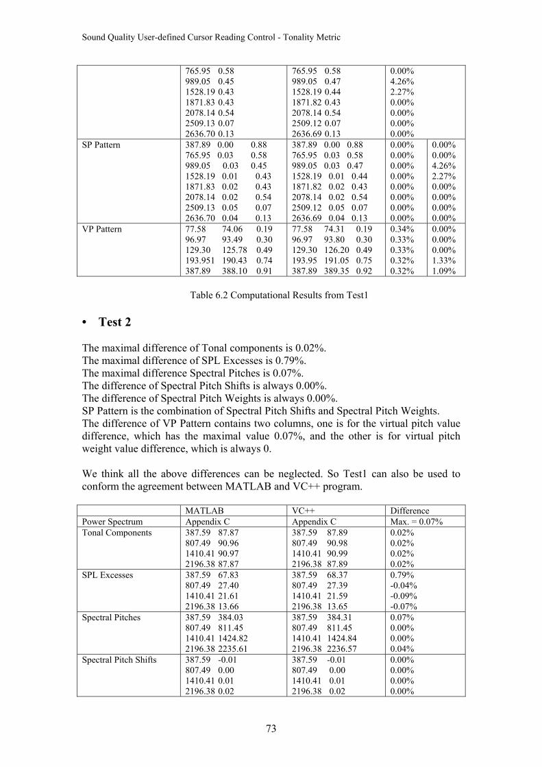
Sound Quality User-defined Cursor Reading Control - Tonality Metric
765.95 0.58 989.05 0.45 1528.19 0.43 1871.83 0.43 2078.14 0.54 2509.13 0.07 2636.70 0.13
765.95 0.58 989.05 0.47 1528.19 0.44 1871.82 0.43 2078.14 0.54 2509.12 0.07 2636.69 0.13
0.00% 4.26% 2.27% 0.00% 0.00% 0.00% 0.00%
SP Pattern
387.89 0.00 0.88 765.95 0.03 0.58 989.05 0.03 0.45 1528.19 0.01 0.43 1871.83 0.02 0.43 2078.14 0.02 0.54 2509.13 0.05 0.07 2636.70 0.04 0.13
387.89 0.00 0.88 765.95 0.03 0.58 989.05 0.03 0.47 1528.19 0.01 0.44 1871.82 0.02 0.43 2078.14 0.02 0.54 2509.12 0.05 0.07 2636.69 0.04 0.13
0.00% 0.00% 0.00% 0.00% 0.00% 0.00% 0.00% 0.00%
0.00% 0.00% 4.26% 2.27% 0.00% 0.00% 0.00% 0.00%
VP Pattern
77.58 74.06 0.19 96.97 93.49 0.30 129.30 125.78 0.49 193.951 190.43 0.74 387.89 388.10 0.91
77.58 74.31 0.19 96.97 93.80 0.30 129.30 126.20 0.49 193.95 191.05 0.75 387.89 389.35 0.92
0.34% 0.33% 0.33% 0.32% 0.32%
0.00% 0.00% 0.00% 1.33% 1.09%
Table 6.2 Computational Results from Test1
• Test 2 The maximal difference of Tonal components is 0.02%. The maximal difference of SPL Excesses is 0.79%. The maximal difference Spectral Pitches is 0.07%. The difference of Spectral Pitch Shifts is always 0.00%. The difference of Spectral Pitch Weights is always 0.00%. SP Pattern is the combination of Spectral Pitch Shifts and Spectral Pitch Weights. The difference of VP Pattern contains two columns, one is for the virtual pitch value difference, which has the maximal value 0.07%, and the other is for virtual pitch weight value difference, which is always 0. We think all the above differences can be neglected. So Test1 can also be used to conform the agreement between MATLAB and VC++ program. MATLAB VC++ Difference Power Spectrum Appendix C Appendix C Max. = 0.07% Tonal Components 387.59 87.87
807.49 90.96 1410.41 90.97 2196.38 87.87
387.59 87.89 807.49 90.98 1410.41 90.99 2196.38 87.89
0.02% 0.02% 0.02% 0.02%
SPL Excesses 387.59 67.83 807.49 27.40 1410.41 21.61 2196.38 13.66
387.59 68.37 807.49 27.39 1410.41 21.59 2196.38 13.65
0.79% -0.04% -0.09% -0.07%
Spectral Pitches
387.59 384.03 807.49 811.45 1410.41 1424.82 2196.38 2235.61
387.59 384.31 807.49 811.45 1410.41 1424.84 2196.38 2236.57
0.07% 0.00% 0.00% 0.04%
Spectral Pitch Shifts
387.59 -0.01 807.49 0.00 1410.41 0.01 2196.38 0.02
387.59 -0.01 807.49 0.00 1410.41 0.01 2196.38 0.02
0.00% 0.00% 0.00% 0.00%
73
Sound Quality User-defined Cursor Reading Control - Tonality Metric
Spectral Pitch Weights 387.59 0.94 807.49 0.84 1410.41 0.71 2196.38 0.48
387.59 0.94 807.49 0.84 1410.41 0.71 2196.38 0.48
0.00% 0.00% 0.00% 0.00%
SP Pattern 387.59 -0.01 0.94 807.49 0.00 0.84 1410.41 0.01 0.71 2196.38 0.02 0.48
387.59 -0.01 0.94 807.49 0.00 0.84 1410.41 0.01 0.71 2196.38 0.02 0.48
0.00% 0.00% 0.00% 0.00%
0.00% 0.00% 0.00% 0.00%
VP Pattern 129.20 124.43 0.33 193.80 188.40 0.36 201.49 195.94 0.31 201.87 197.61 0.37 387.59 384.03 0.37
129.20 124.52 0.33 193.80 188.54 0.36 201.49 195.94 0.31 201.87 197.61 0.37 387.59 384.31 0.37
0.07% 0.07% 0.00% 0.00% 0.07%
0.00% 0.00% 0.00% 0.00% 0.00%
Table 6.3 Computational Results from Test2
From Test 1 and Test 2, we can see that the relevant results for both MATLAB and VC++ code agree with each other very well, even though they have some different Power Spectrum as input data. So that the two programs are validated.
74
Sound Quality User-defined Cursor Reading Control - Tonality Metric
Chapter 7 Further Study This chapter introduces Loudness and Aures’s Model of Tonality. The Psychoacoustic concepts, which are used in Loudness such as masking patterns, critical bands, bark scale, we have introduced in chapter 2. The Stationary Loudness model is built as a MATLAB library and tested with a set of reference signals. 7.1 Loudness Loudness is a description of how human beings perceives the physical sound pressure level of a sound. A computational model for loudness must take some of the main properties of our hearing into account. The most important ones are masking, frequency selectivity, threshold in quiet and on accounting for frontal (free) sound field and diffuse sound field (Zwicker, 1981).
7.1.1 Stationary Loudness and Non-stationary Loudness There are two types of loudness – stationary loudness for stationary signals and non-stationary loudness for non-stationary signals.
• A stationary signal is a signal that is perceived by a human as not to change over time. For example: noise from waterfall or a tone at constant level. The stationary loudness is described in ISO 532 and DIN 45632, and DIN45632 is based on the BASIC computer program contained in the German standard DIN 45631,1991.
• Non-Stationary signals are signals that are perceived to change over time. For
example: transient signals, like a hammer hitting a nail, and modulating signals, like an alternating ambulance horn. Currently there is no standard for the calculation of non-stationary loudness. According to Poul Ladegaard, Brüel & Kjær, a standard for non-stationary Loudness is not finished yet. An International committee is working on to standardize it. It is expect to be standardized within half a year.
7.1.2 Method A and Method B for Stationary Loudness There are two methods for calculating Stationary Loudness, according to the international Standard ISO 532.
• The first Method A, referred to as Stevens method, utilizes physical measurement obtained from spectrum analysis in terms of octave bands.
• The second Method B, referred to as Zwicker’s method, utilizes spectrum
analysis in terms of one-third octave bands.
Method B, which is for Stationary Loudness, is the widely used method in Sound Quality field and also more complex than the Stevens method A. Method B provides
75
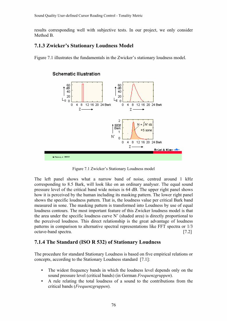
Sound Quality User-defined Cursor Reading Control - Tonality Metric
results corresponding well with subjective tests. In our project, we only consider Method B.
7.1.3 Zwicker’s Stationary Loudness Model Figure 7.1 illustrates the fundamentals in the Zwicker’s stationary loudness model.
Figure 7.1 Zwicker’s Stationary Loudness model The left panel shows what a narrow band of noise, centred around 1 kHz corresponding to 8.5 Bark, will look like on an ordinary analyser. The equal sound pressure level of the critical band wide noises is 64 dB. The upper right panel shows how it is perceived by the human including its masking pattern. The lower right panel shows the specific loudness pattern. That is, the loudness value per critical Bark band measured in sone. The masking pattern is transformed into Loudness by use of equal loudness contours. The most important feature of this Zwicker loudness model is that the area under the specific loudness curve N’ (shaded area) is directly proportional to the perceived loudness. This direct relationship is the great advantage of loudness patterns in comparison to alternative spectral representations like FFT spectra or 1/3 octave-band spectra. [7.2]
7.1.4 The Standard (ISO R 532) of Stationary Loudness The procedure for standard Stationary Loudness is based on five empirical relations or concepts, according to the Stationary Loudness standard [7.1]:
• The widest frequency bands in which the loudness level depends only on the sound pressure level (critical bands) (in German Frequenzgruppen).
• A rule relating the total loudness of a sound to the contributions from the critical bands (Frequenzgruppen).
76
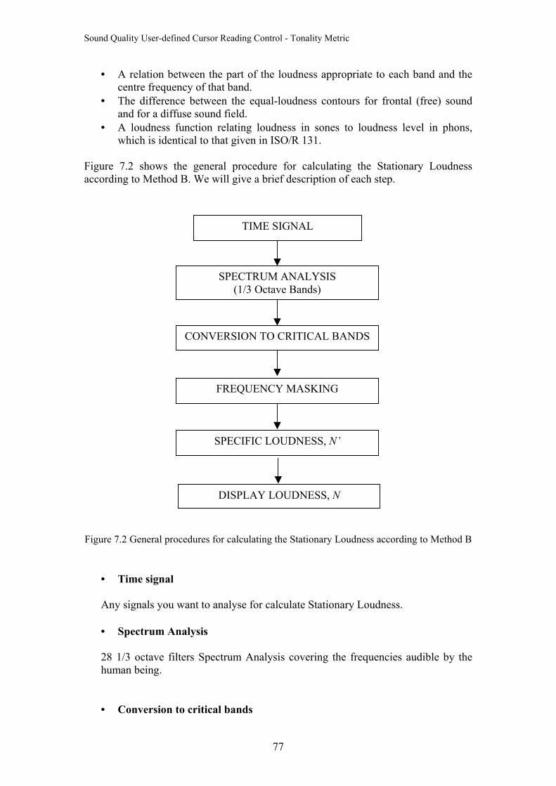
Sound Quality User-defined Cursor Reading Control - Tonality Metric
• A relation between the part of the loudness appropriate to each band and the centre frequency of that band.
• The difference between the equal-loudness contours for frontal (free) sound and for a diffuse sound field.
• A loudness function relating loudness in sones to loudness level in phons, which is identical to that given in ISO/R 131.
Figure 7.2 shows the general procedure for calculating the Stationary Loudness according to Method B. We will give a brief description of each step.
SPECTRUM ANALYSIS (1/3 Octave Bands)
CONVERSION TO CRITICAL BANDS
FREQUENCY MASKING
SPECIFIC LOUDNESS, N’
DISPLAY LOUDNESS, N
TIME SIGNAL Figure 7.2 General procedures for calculating the Stationary Loudness according to Method B
• Time signal Any signals you want to analyse for calculate Stationary Loudness.
• Spectrum Analysis 28 1/3 octave filters Spectrum Analysis covering the frequencies audible by the human being. • Conversion to critical bands
77

Sound Quality User-defined Cursor Reading Control - Tonality Metric
Above 500 Hz, critical bands are approximately one-third octave in width. Since the lower one-third octave filters are narrower than 100 Hz, the bands below 500 Hz are combined to approximate critical bands. The 28 1/3 Octave bands are combined to the critical bands in the following way. In the lowest frequency region, the one-third octave bands with centre frequencies from 25 to 80 Hz are combined to form the first band. The one-third octave bands from 100 to 160 Hz are combined to form the next band. The 200 and 250 Hz bands are combined. The bands from 315 to 12500 Hz are used individually, since their bandwidths approximate critical bands. The DIN 45631 standard describes how to obtain values for critical banded based on one-third octave bands. • Frequency masking After conversion from 28 1/3 octave bands into 20 Critical bands a correction is applied depending whether the environment is a free or diffuse field. The SPL values are then converted into loudness values and frequency masking is applied. The frequency masking is only for the masking of higher critical bands by lower critical bands. The masking of lower critical bands is considered to be negligible. • Specific Loudness, N’ Each critical band can be displayed as a specific loudness spectrum, N’. • Display Loudness, N
We display all bands of specific loudness summed into a single number as stationary loudness (Total Loudness), N.
Figure7.3 shows how the Stationary Loudness spectrum displays in B&K SQ Application. Total Loudness is the sum of Specific Loudness. The curved line represents frequency masking. The Stationary Loudness is the area under the curve.
78
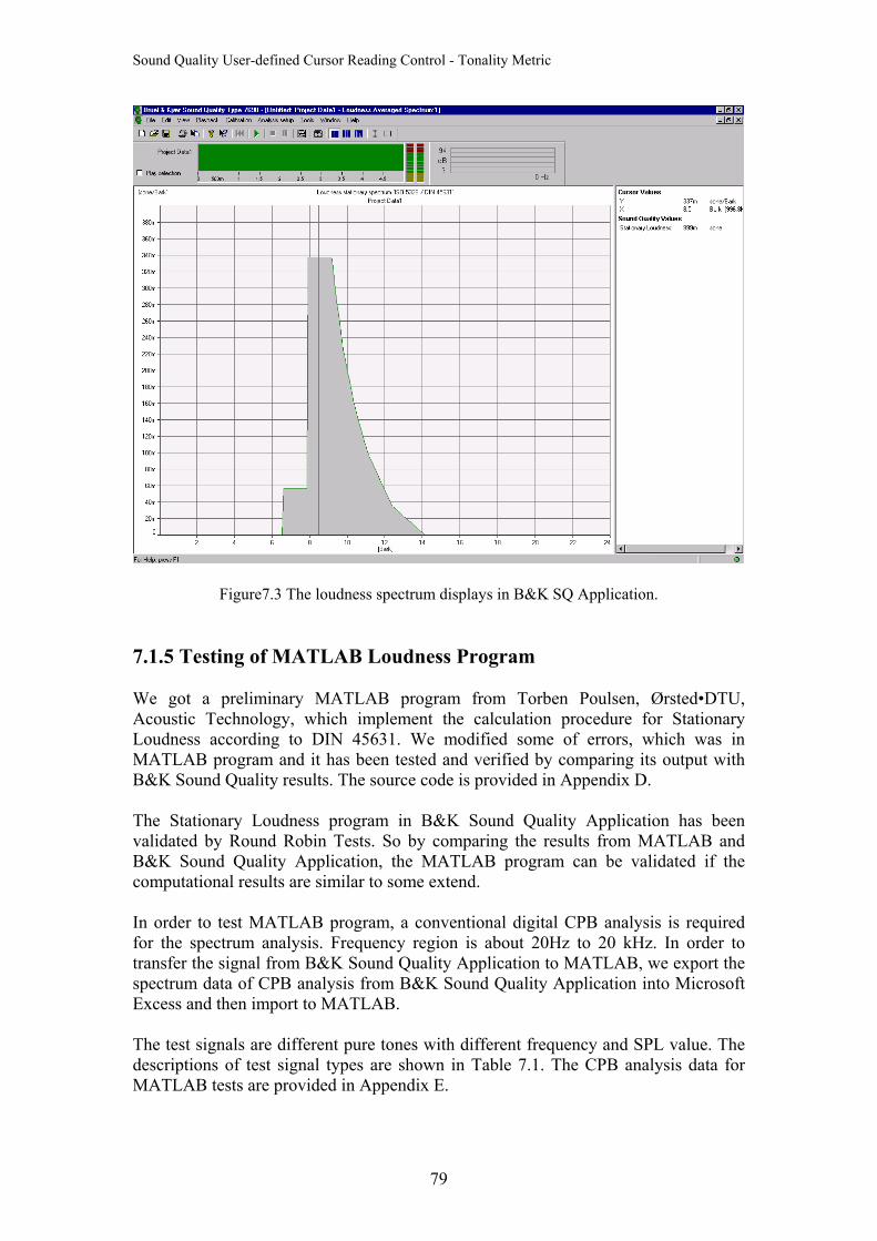
Sound Quality User-defined Cursor Reading Control - Tonality Metric
Figure7.3 The loudness spectrum displays in B&K SQ Application.
7.1.5 Testing of MATLAB Loudness Program We got a preliminary MATLAB program from Torben Poulsen, Ørsted•DTU, Acoustic Technology, which implement the calculation procedure for Stationary Loudness according to DIN 45631. We modified some of errors, which was in MATLAB program and it has been tested and verified by comparing its output with B&K Sound Quality results. The source code is provided in Appendix D. The Stationary Loudness program in B&K Sound Quality Application has been validated by Round Robin Tests. So by comparing the results from MATLAB and B&K Sound Quality Application, the MATLAB program can be validated if the computational results are similar to some extend. In order to test MATLAB program, a conventional digital CPB analysis is required for the spectrum analysis. Frequency region is about 20Hz to 20 kHz. In order to transfer the signal from B&K Sound Quality Application to MATLAB, we export the spectrum data of CPB analysis from B&K Sound Quality Application into Microsoft Excess and then import to MATLAB. The test signals are different pure tones with different frequency and SPL value. The descriptions of test signal types are shown in Table 7.1. The CPB analysis data for MATLAB tests are provided in Appendix E.
79
Sound Quality User-defined Cursor Reading Control - Tonality Metric
The following table contains the test results for Stationary Loudness from B&K Sound Quality type 7698 and MATLAB.
Loudness (unit: sone)
B&K SQ MATLAB Difference
No
Signal type
Loudness
in Theory
( ) ≈ Free (F1)
Diffuse (D1)
Free (F2)
Diffuse (D2)
|F2-F1|/F1 |D2-D1|/D1
1 Pure Tone at 1kHz of
40 dB
1
0,99
1,26
1,0
1,3
1.01%
3.17%
2 Pure Tone at 2kHz of
80 dB
19
19,4
17,9
19,3
17,9
0.52%
0.00%
3 Pure Tone at 4kHz of
80 dB
24
24,6
22,8
24,0
22,5
2.44%
1.32%
4 Pure Tone at 8kHz of
80 dB
13
13,1
16,5
12,6
15,8
3.82%
4.24%
Table 7.1 Test Result from the Stationary Loudness
Table 7.1 shows that the maximal difference of Stationary Loudness result in free field is 3.82%, and the maximal difference of Stationary Loudness result in diffuse field is 4.24%. The difference is acceptable, because we think it is courses by the different programming languages and the fact that the input data to MATLAB is slightly different from the Sound Quality Application. Besides the calculation results for Stationary Loudness, MATLAB program can also show some spectrums. Figure 7.4 shows the spectrum when we made the first test.
Figure 7.4 Stationary Loudness Test Spectrum for a pure tone at 1 kHz 40 dB in MATLAB
80
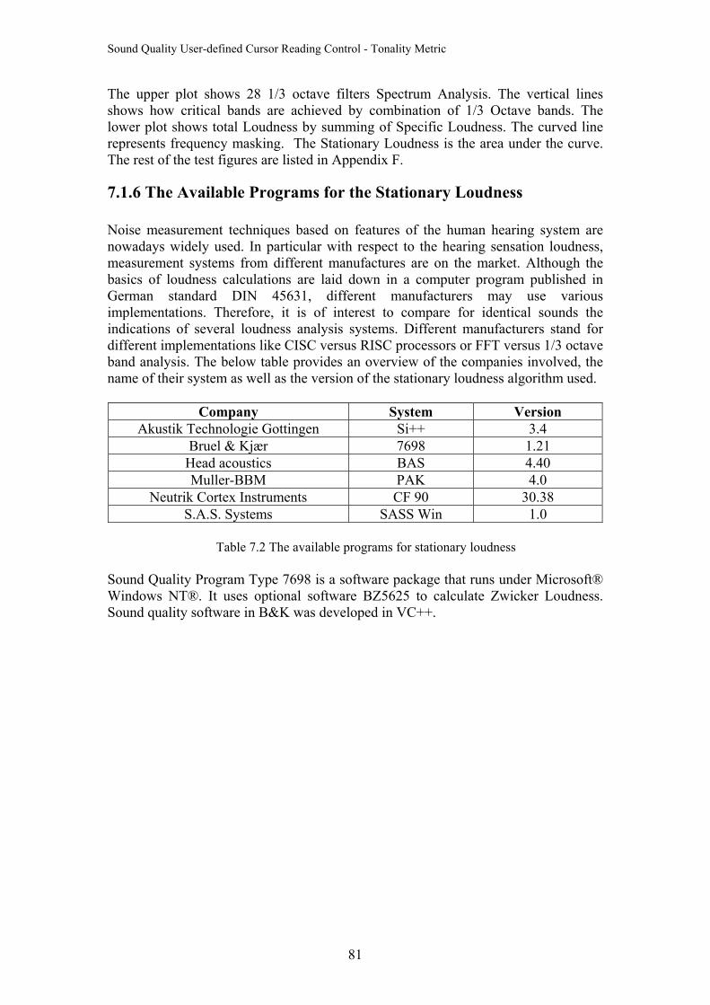
Sound Quality User-defined Cursor Reading Control - Tonality Metric
The upper plot shows 28 1/3 octave filters Spectrum Analysis. The vertical lines shows how critical bands are achieved by combination of 1/3 Octave bands. The lower plot shows total Loudness by summing of Specific Loudness. The curved line represents frequency masking. The Stationary Loudness is the area under the curve. The rest of the test figures are listed in Appendix F.
7.1.6 The Available Programs for the Stationary Loudness Noise measurement techniques based on features of the human hearing system are nowadays widely used. In particular with respect to the hearing sensation loudness, measurement systems from different manufactures are on the market. Although the basics of loudness calculations are laid down in a computer program published in German standard DIN 45631, different manufacturers may use various implementations. Therefore, it is of interest to compare for identical sounds the indications of several loudness analysis systems. Different manufacturers stand for different implementations like CISC versus RISC processors or FFT versus 1/3 octave band analysis. The below table provides an overview of the companies involved, the name of their system as well as the version of the stationary loudness algorithm used.
Company System Version Akustik Technologie Gottingen Si++ 3.4
Bruel & Kjær 7698 1.21 Head acoustics BAS 4.40 Muller-BBM PAK 4.0
Neutrik Cortex Instruments CF 90 30.38 S.A.S. Systems SASS Win 1.0
Table 7.2 The available programs for stationary loudness
Sound Quality Program Type 7698 is a software package that runs under Microsoft® Windows NT®. It uses optional software BZ5625 to calculate Zwicker Loudness. Sound quality software in B&K was developed in VC++.
81
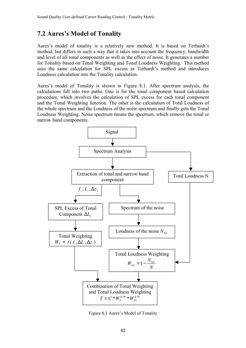
Sound Quality User-defined Cursor Reading Control - Tonality Metric
7.2 Aures’s Model of Tonality Aures’s model of tonality is a relatively new method. It is based on Terhardt’s method, but differs in such a way that it takes into account the frequency, bandwidth and level of all tonal components as well as the effect of noise. It generates a number for Tonality based on Tonal Weighting and Tonal Loudness Weighting. This method uses the same calculation for SPL excess as Terhardt’s method and introduces Loudness calculation into the Tonality calculation. Aures’s model of Tonality is shown in Figure 8.1. After spectrum analysis, the calculations fall into two paths. One is for the tonal component based calculation procedure, which involves the calculation of SPL excess for each tonal component and the Tonal Weighting function. The other is the calculation of Total Loudness of the whole spectrum and the Loudness of the noise spectrum and finally gets the Tonal Loudness Weighting. Noise spectrum means the spectrum, which remove the tonal or narrow band components.
Signal
Spectrum Analysis
Extraction of tonal and narrow band component
iii zLf ∆,,
SPL Excess of Tonal Component iL∆
Spectrum of the noise
Loudness of the noise GrN ),,( iiiT zLffW ∆∆=
Tonal Loudness Weighting
NN
W GrGr −=1
Total Loudness N
Combination of Tonal Weightingand Tonal Loudness Weighting
79.029.0 ** GrT WWCT =
Tonal Weighting
Figure 8.1 Aures’s Model of Tonality
82
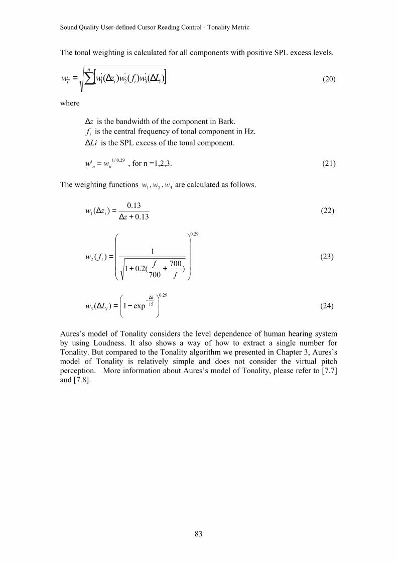
Sound Quality User-defined Cursor Reading Control - Tonality Metric
The tonal weighting is calculated for all components with positive SPL excess levels.
[ ]∑ ∆∆=n
iiiT Lwfwzww )()()( '3
'2
'1 (20)
where
is the bandwidth of the component in Bark. z∆ is the central frequency of tonal component in Hz. if is the SPL excess of the tonal component. Li∆
, for n =1,2,3. (21) 29.0/1' nn ww = The weighting functions are calculated as follows. 321 ,, www
13.013.0)(1 +∆
=∆z
zw i (22)
29.0
2
)700700
(2.01
1)(
++=
ff
fw i (23)
29.0
153 exp1)(
−=∆
∆− l
iLw (24)
Aures’s model of Tonality considers the level dependence of human hearing system by using Loudness. It also shows a way of how to extract a single number for Tonality. But compared to the Tonality algorithm we presented in Chapter 3, Aures’s model of Tonality is relatively simple and does not consider the virtual pitch perception. More information about Aures’s model of Tonality, please refer to [7.7] and [7.8].
83
Sound Quality User-defined Cursor Reading Control - Tonality Metric
Chapter 8 Conclusions and Further work The work carried out in this thesis can be described as four major parts. The first part is the study of Terhardt’s Tonality algorithm and the simulation of the algorithm by using MATLAB. The second part is the study of ATL COM programming in order to make a metric for B&K SQ Application, and the implementation of Terhardt’s Tonality algorithm in VC++. The third part is the testing of MATLAB and VC++ code by showing the consistency of the computational results. The fourth part is the study of Stationary Loudness and Aures’s model of Tonality. Simulating the algorithm in MATLAB helped us to understand the calculation procedure in detail, and proved that the algorithm could be implemented according to our Data Flow analysis. The experience of VC++ programming for Tonality metric gave us an opportunity to learn how COM technology being used in B&K Sound Quality Application, and how the same algorithm can be implemented using different programming languages. Testing results showed that the computational results agree with each other, so that our VC++ code is ready to be used in B&K Sound Quality Application for further research or development work. The study of Stationary Loudness and Aures’s model of Tonality made us understand how psychoacoustics concepts are being used in Loudness and Tonality and brought us some fresh ideas for further discussion. We think the following work can be considered and carried out based on our thesis project. • Extract a single number and make subjective test for Tonality A single number for Tonality means it could statistically show the proportional relationship between Tonality metric and the tonal perception of human hearing system for a signal, which has the tonal attribute. The Tonality algorithm used in this thesis described that in an actual listening situation, the whole pitch percept is described as a competition between spectral and virtual pitches. These two types of pitches are extracted from the signal and represented by the spectral-pitch pattern and the virtual-pitch pattern. The evaluation of the competition between spectral and virtual pitches becomes the important issues in order to extract a single number for Tonality. We are sure our MATLAB model can help to evaluate the competition, but further work need to be done in order to find a way to extract a single number for Tonality. For example, by finding a weighting function, which can be applied on both spectral-pattern and virtual- pitch pattern, the single number for Tonality can be extracted. This should be correlated with results from subjective test.
• Improve Tonality by using parts of the Loudness Model Mutual masking of spectral components has been evaluated in the Tonality algorithm through the calculation procedures for sound-pressure level excess and pitch shifts. The Stationary Loudness is an ISO Standard, which evaluate the masking effects based on Critical Bands and finally get a single number for Loudness from the specific Loudness. The single number we get from Loudness contains the overall information of how human being perceives the physical sound pressure level of a
84
Sound Quality User-defined Cursor Reading Control - Tonality Metric
sound. So if we can find a right way to introduce Loudness into Tonality, the calculation of Tonality will have more precision, better correlation with subjective results and more standardized evaluation of masking effects. Aures’s model is an example of trying to combine Tonality and Loudness. But we think they use Tonality in a very simple way, which is not enough to evaluate the tonal aspects of a sound. Aures’s model can be built based on our Tonality MATLAB model and the Loudness MATLAB Model for further research work. • Tonality for Non-stationary signal Terhardt’s Tonality algorithm, which we discussed in Chapter 3, is a pitch-evaluation procedure for any complex tone. The algorithm can work well with stationary signals, but for non-stationary signals it might have some drawbacks. For example, it will evaluate a strong tonal component as a non-tonal component if the frequency of the tone changes with time. The reason is the spectrum from FFT analysis of a non-stationary signal might merge some discrete tonal contents which can be seen in time domain, and show them as non-tonal contents in frequency domain. By assuming that the time signal can be composed by a sequence of short duration signal, we can divide the non-stationary signal into some small time blocks. Each of them can be understood as a stationary signal when the time duration is small enough. Next, evaluate each of them by using the Tonality algorithm. In the end, you will get a spectral pitch pattern and virtual pitch pattern for each short duration signal, which you can show together in a contour or waterfall graph with both frequency and time axis. Inspecting the graph more tones may show up and contribute to the overall Tonality compared to just analysing a single spectrum. • Improvement of Tonality VC++ code The Tonality metric implementation in VC++ follows the general routines of making a user-defined cursor reading control. It is the same as how B&K SQ customers make their own metrics for SQ Application. The main idea of this program structure is to simplify the connection between the user-defined metric and the main SQ program. B&K also has some metrics developed inside SQ program, which all provide the function of showing the spectrums and contours. These functions are very hard to implement by using ATL COM programming. But by embedding Tonality as a part of main SQ program, more functions can be provided for the customers, such as showing the spectrum-pitch pattern and virtual-pitch pattern in a spectrum. We suggest that Tonality should be implemented as a part of SQ main program if one day it becomes part of the commercial software.
85
Sound Quality User-defined Cursor Reading Control - Tonality Metric
Bibliography [1.1] Joseph Emmanuel Amuah, “Sound Quality User-defined Cursor Reading Controls”, Master Thesis, IMM, DTU, Lyngby, Denmark. June 2002 [2.1] E. Zwicker, H. Fastel: Psychoacoustics, Facts and Models, Springer-Verlag Berlin Heidelberg 1999. [2.2] B&KA/S, Lecture notes ‘Basic Concepts of Sound’ [2.3] B&KA/S, Lecture notes ‘Basic Frequency Analysis of Sound’ [2.4] B&KA/S, Lecture notes ‘Sound Quality Equalisation and Calibration’ [2.5] B&KA/S, Guided Tour - System Calibration, Sound Recording and Playback [2.6] B&KA/S, Lecture notes ‘Psychoacoustics – a qualitative description’. [2.7] B&KA/S, Lecture notes ‘Introduction to Sound Quality’. [2.8] http://www2.egr.uh.edu/~glover/applets/Sampling/Sampling.html (1/10/2002). [2.9] http://www.ihear.com/Pitch/paradoxical.html (1/10/2002). [2.10] http://acoustics.auc.dk/research/SQRU/index.php Sound Quality Research Unit (15/10/2002) [2.11] http://www.sfu.ca/sonic-studio/handbook/index.html Handbook For Acoustic Ecology. (20/10/2002) [3.1] Terhardt, E., Stoll, G., and Seewann, M.(1982). “An algorithm for extraction of pitch and pitch salience from complex tonal signals,” J. Acoust. Soc. Am. 71, 679-688. [3.2] Terhardt, E., Stoll, G., and Seewann, M.(1982). “Pitch of complex signals according to virtual-pitch theory: Test, examples, and predictions,” J. Acoust. Soc. Am. 71, 671-678. [3.3] International Standard ISO 532 Acoustics-Method for calculating loudness level. [4.1] MATLAB Help [5.1] Richard Grimes, Beginning ATL 3 COM Programming, Wrox Press, Birmingham, UK, 1999. [5.2] Stanley B. Lippman, Josee Lajoie, C++ Primer, Addison-Wesley, Canada, 1999. [5.3] The Microsoft Developer Network (MSDN) Library, October 2001. [5.4] David J.Kruglinski, Inside Visual C++ , Microsoft Press, Washington, 1993. [5.5] Bjarne Stroustrup, The C++ Programming Language, Second Edition, AT&T Bell Laboratories, Murray Hill, New Jersey, 1992. [7.1] E.Zwicker and H.Fastl, Psychoacoustics. Springer Verlag, 2nd ed.,1999 [7.2] B&Ksoftware, Sound Quality type 7698 [7.3] May, P.G., “Assessment of Refrigerator Sound Quality”, Purdue University, 1998. [7.4] International standard ISO 131, [7.5] International standard ISO 532, Acoustics –Method for calculation loudness level, 1st ed., 1975 [7.6] Brüel & Kjær, “Psychoacoustics”, Lecture, BA 7615-13. [7.7] W.Aures, Procedure for Calculating the Sensory Euphony of Arbitrary Sound Signals, Acusitca 59, 130-141, 1985.
86

Sound Quality User-defined Cursor Reading Control - Tonality Metric
[7.8]Aaron Hastings and Patricia Davies, An examination of Aures’s model of Tonality, InterNoise 2002.
87

Sound Quality User-defined Cursor Reading Control - Tonality Metric
Appendix A MATLAB Source Code for Tonality
88

Sound Quality User-defined Cursor Reading Control - Tonality Metric
Appendix B VC++ Source Code for Tonality
89
Sound Quality User-defined Cursor Reading Control - Tonality Metric
Appendix C Power Spectrum Data for Test1 and Test2 Test1: Maximal SPL Difference = 0.19% Test2: Maximal SPL Difference = 0.07%
Power Spectrum of Test 1 Power Spectrum of Test 2 MATLAB VC++ MATLAB VC++
Freq. (Hz)
SPL1 (dB)
Freq. (Hz)
SPL2 (dB)
(SPL2-SPL1) /SPL2
Freq. (Hz)
SPL3 (dB)
Freq. (Hz)
SPL4 (dB)
(SPL4-SPL3) /SPL4
0.00 10.77 21.53 32.30 43.07 53.83 64.60 75.37 86.13 96.90 107.67 118.43 129.20 139.97 150.73 161.50 172.27 183.03 193.80 204.57 215.33 226.10 236.87 247.63 258.40 269.17 279.93 290.70 301.47 312.23 323.00 333.76 344.53 355.30 366.06 376.83 387.60 398.36 409.13 419.90 430.66 441.43 452.20 462.96 473.73 484.50 495.26
56.28 54.37 47.19 42.95 38.71 34.79 30.68 30.96 34.44 47.69 56.08 56.83 56.25 55.49 54.61 51.36 42.02 34.99 35.80 45.26 53.91 54.98 53.77 55.36 57.31 55.94 51.85 49.88 48.31 47.14 52.91 55.15 53.04 53.03 54.09 56.31 58.13 56.95 53.23 51.32 54.41 54.67 50.90 48.38 46.08 46.07 45.04
0.00 10.77 21.53 32.30 43.07 53.83 64.60 75.37 86.13 96.90 107.67 118.43 129.20 139.97 150.73 161.50 172.27 183.03 193.80 204.57 215.33 226.10 236.87 247.63 258.40 269.17 279.93 290.70 301.46 312.23 323.00 333.76 344.53 355.30 366.06 376.83 387.60 398.36 409.13 419.90 430.66 441.43 452.20 462.96 473.73 484.50 495.26
56.30 54.39 47.21 42.97 38.73 34.81 30.70 30.98 34.46 47.71 56.10 56.85 56.27 55.51 54.63 51.38 42.04 35.01 35.82 45.28 53.93 55.00 53.79 55.38 57.33 55.96 51.87 49.90 48.33 47.16 52.93 55.17 53.06 53.05 54.11 56.33 58.15 56.97 53.25 51.34 54.43 54.69 50.92 48.40 46.10 46.09 45.06
0.00 10.77 21.53 32.30 43.07 53.83 64.60 75.37 86.13 96.90 107.67 118.43 129.20 139.97 150.73 161.50 172.27 183.03 193.80 204.57 215.33 226.10 236.87 247.63 258.40 269.17 279.93 290.70 301.46 312.23 323.00 333.76 344.53 355.30 366.06 376.83 387.60 398.36 409.13 419.90 430.66 441.43 452.20 462.96 473.73 484.50 495.26
51.51 50.44 48.99 48.95 49.78 50.28 50.37 49.12 49.38 49.36 48.95 48.89 47.49 49.62 49.37 49.34 49.05 49.31 49.07 49.17 48.93 48.95 48.98 49.20 48.75 48.89 49.29 49.27 49.77 49.19 48.96 49.29 49.30 48.82 49.11 81.88 87.89 81.87 49.42 48.71 49.35 49.57 49.17 49.43 49.74 48.87 48.73
0.04% 0.04% 0.04% 0.04% 0.04% 0.04% 0.04% 0.04% 0.04% 0.04% 0.04% 0.04% 0.04% 0.06% 0.04% 0.04% 0.04% 0.04% 0.04% 0.04% 0.04% 0.04% 0.04% 0.04% 0.06% 0.04% 0.04% 0.06% 0.04% 0.06% 0.04% 0.04% 0.04% 0.04% 0.04% 0.02% 0.02% 0.02% 0.06% 0.04% 0.04% 0.04% 0.04% 0.04% 0.04% 0.06% 0.04%
0.04% 0.04% 0.04% 0.05% 0.05% 0.06% 0.07% 0.06% 0.06% 0.04% 0.04% 0.04% 0.04%
0.04% 0.04% 0.05% 0.06% 0.06% 0.04% 0.04% 0.04% 0.04% 0.04% 0.03% 0.04% 0.04% 0.04% 0.04% 0.04% 0.04% 0.04% 0.04% 0.04% 0.04% 0.04% 0.03% 0.04% 0.04% 0.04%
0.04% 0.04% 0.04% 0.04% 0.04% 0.04%
0.00 51.49 10.77 50.42 21.53 32.30 43.07
96.90 107.67 118.43 129.20 139.97 150.73 161.50 172.27 183.03 193.80
215.33 226.10 236.87 247.63 258.40 269.17 279.93 290.70 301.47 312.23 323.00 333.76 344.53 355.30 366.06 376.83
398.36 409.13 419.90 430.66 441.43 452.20 462.96 473.73 484.50 495.26
48.97 48.93 49.76
53.83 50.26 64.60 50.35 75.37 49.10 86.13 49.36
49.34 48.93 48.87 47.47
0.04% 49.59 49.35 49.32 49.03 49.29 49.05
204.57 49.15 48.91 48.93 48.96 49.18 48.72 48.87 49.27 49.24 49.75 49.16 48.94 49.27 49.28 48.80 49.09 81.86
387.60 87.87 81.85 49.39 48.69
0.04% 49.33 49.55 49.15 49.41 49.72 48.84 48.71
90
Sound Quality User-defined Cursor Reading Control - Tonality Metric
506.03 516.80 527.56 538.33 549.10 559.86 570.63 581.40 592.16 602.93 613.70 624.46 635.23 646.00 656.76 667.53 678.30 689.06 699.83 710.60 721.36 732.13 742.90 753.66 764.43 775.20 785.96 796.73 807.50 818.26 829.03 839.80 850.56 861.33 872.10 882.86 893.63 904.39 915.16 925.93 936.69 947.46 958.23 968.99 979.76 990.53 1001.29 1012.06 1022.83 1033.59 1044.36 1055.13 1065.89 1076.66 1087.43 1098.19 1108.96 1119.73 1130.49 1141.26
42.25 40.51 39.39 39.47 41.97 39.32 35.92 35.76 35.02 33.09 32.97 33.56 33.92 36.16 36.28 33.01 29.53 26.61 26.21 26.77 26.69 25.71 24.87 28.68 33.20 31.98 29.53 28.79 25.52 24.34 25.68 24.06 21.94 22.57 25.21 24.33 22.55 22.04 22.72 21.64 20.04 19.73 20.96 21.95 25.52 26.51 22.31 20.94 20.05 22.58 22.70 19.50 19.91 22.77 22.72 22.43 20.85 20.57 19.32 18.68
506.03 516.80 527.56 538.33 549.10 559.86 570.63 581.40 592.16 602.93 613.70 624.46 635.23 646.00 656.76 667.53 678.30 689.06 699.83 710.60 721.36 732.13 742.90 753.66 764.43 775.20 785.96 796.73 807.50 818.26 829.03 839.79 850.56 861.33 872.09 882.86 893.63 904.39 915.16 925.93 936.69 947.46 958.23 968.99 979.76 990.53 1001.29 1012.06 1022.83 1033.59 1044.36 1055.13 1065.89 1076.66 1087.43 1098.19 1108.96 1119.731130.49 1141.26
42.27 40.53 39.41 39.49 41.99 39.34 35.94 35.78 35.04 33.11 32.99 33.58 33.94 36.19 36.30 33.03 29.55 26.64 26.23 26.79 26.71 25.73 24.89 28.70 33.22 32.01 29.55 28.81 25.54 24.36 25.70 24.08 21.96 22.59 25.24 24.35 22.57 22.06 22.74 21.66 20.06 19.75 20.98 21.97 25.54 26.53 22.33 20.96 20.07 22.60 22.72 19.52 19.93 22.79 22.74 22.45 20.87 20.59 19.34 18.70
49.61 48.45
48.86 48.34 48.34 84.97 90.96 84.96 49.82 48.84 48.51
49.57 48.80 48.80 48.45 48.17 48.66 49.15
49.61
48.50 49.09 49.70 50.09 49.21 48.95 49.62
49.20 50.23 49.13 48.97 49.44 50.00 49.14 48.68 49.49 49.69 49.12
506.03 516.80 527.56 538.33 549.10 559.86 570.63 581.40 592.16 602.93 613.70 624.46 635.23 646.00 656.76 667.53 678.30 689.06 699.83 710.60 721.36 732.13 742.90 753.66 764.43 775.20 785.96 796.73 807.50 818.26 829.03 839.79 850.56 861.33 872.09 882.86 893.63 904.39 915.16 925.93 936.69 947.46 958.23 968.99 979.76 990.53 1001.29 1012.06 1022.83 1033.59 1044.36 1055.13 1065.89 1076.66 1087.43 1098.19 1108.96 1119.731130.49 1141.26
48.63 48.64 48.81 49.02 49.95 49.60 49.25 49.63 49.85 49.88 50.26 49.52 48.38 49.55 49.90 49.29 49.40 49.57 49.41 49.12 50.00 49.63 48.47 49.15 48.88 48.36 48.36 84.99 90.98 84.98 49.84 48.86 48.53 49.27 49.59 48.82 48.82 48.47 48.19 48.68 49.17 48.52 49.11 49.72 50.11 49.23 48.97 49.64 49.63 49.22 50.25 49.16 48.99 49.46 50.02 49.16 48.70 49.51 49.71 49.14
0.04% 0.04% 0.04% 0.04% 0.04% 0.04% 0.04% 0.04% 0.04% 0.04% 0.06% 0.04% 0.04% 0.04% 0.04% 0.04% 0.04% 0.04% 0.04% 0.04% 0.06% 0.04% 0.04% 0.04% 0.04% 0.04% 0.04% 0.02% 0.02% 0.02% 0.04% 0.04% 0.04% 0.04% 0.04% 0.04% 0.04% 0.04% 0.04% 0.04% 0.04% 0.04% 0.04% 0.04% 0.04% 0.04% 0.04% 0.04% 0.04% 0.04% 0.04% 0.06% 0.04% 0.04% 0.04% 0.04% 0.04% 0.04% 0.04% 0.04%
0.05% 0.05% 0.05% 0.05% 0.05% 0.05% 0.06% 0.06% 0.06% 0.06% 0.06% 0.06% 0.06% 0.08% 0.06% 0.06% 0.07% 0.11% 0.08% 0.07% 0.07% 0.08% 0.08% 0.07% 0.06% 0.09% 0.07% 0.07%
0.08% 0.08% 0.08% 0.09% 0.09% 0.12% 0.08% 0.09% 0.09% 0.09% 0.09% 0.10% 0.10% 0.10% 0.09% 0.08% 0.08% 0.09% 0.10% 0.10% 0.09% 0.09%
506.03 516.80 527.56 538.33 549.10 559.86
581.40 592.16 602.93 613.70 624.46 635.23 646.00 656.76 667.53 678.30 689.06 699.83 710.60 721.36 732.13 742.90
764.43 775.20 785.96 796.73 807.50 818.26 829.03 839.80 850.56 861.33 872.10 882.86 893.63 904.39 915.16 925.93 936.69
48.61 48.62 48.79 49.00 49.93 49.58
570.63 49.23 49.61 49.83 49.86 50.23 49.50 48.36 49.53 49.88 49.27 49.38 49.55 49.39 49.10 49.97
753.66 49.13
0.08%
49.25
947.46 958.23 968.99 979.76 990.53 1001.29 1012.06 1022.83 1033.59 1044.36
0.10% 1055.13 0.10% 1065.89 0.09% 1076.66 0.09% 1087.43 0.09% 1098.19 0.10% 1108.96 0.10%0.10%
1119.73 1130.49 1141.26 0.11%
91
Sound Quality User-defined Cursor Reading Control - Tonality Metric
1152.03 1162.79 1173.56 1184.33 1195.09 1205.86 1216.63 1227.39 1238.16 1248.93 1259.69 1270.46 1281.23 1291.99 1302.76 1313.53 1324.29 1335.06 1345.83 1356.59 1367.36 1378.13 1388.89 1399.66 1410.42 1421.19 1431.96 1442.72 1453.49 1464.26 1475.02 1485.79 1496.56 1507.32 1518.09 1528.86 1539.62 1550.39 1561.16 1571.92 1582.69 1593.46 1604.22 1614.99 1625.76 1636.52 1647.29 1658.06 1668.82 1679.59 1690.36 1701.12 1711.89 1722.66 1733.42 1744.19 1754.96 1765.72 1776.49 1787.26
19.10 21.58 20.80 20.60 23.33 24.91 25.30 23.82 19.21 18.59 17.33 19.60 21.23 21.51 22.18 21.59 20.09 20.38 20.45 19.54 17.82 16.24 18.23 18.91 23.24 24.04 23.11 22.49 24.38 24.46 23.97 21.65 20.05 19.56 25.57 27.16 24.12 23.79 23.55 24.45 25.49 27.21 25.57 23.45 26.43 28.37 25.76 24.92 27.50 25.97 25.02 29.02 30.64 28.23 28.54 33.55 32.50 25.36 27.82 28.57
1152.03 1162.79 1173.56 1184.33 1195.09 1205.86 1216.63 1227.39 1238.16 1248.93 1259.69 1270.46 1281.23 1291.99 1302.76 1313.53 1324.29 1335.06 1345.83 1356.59 1367.36 1378.13 1388.89 1399.66 1410.42 1421.19 1431.96 1442.72 1453.49 1464.26 1475.02 1485.79 1496.56 1507.32 1518.09 1528.86 1539.62 1550.39 1561.16 1571.92 1582.69 1593.46 1604.22 1614.99 1625.76 1636.52 1647.29 1658.06 1668.82 1679.59 1690.36 1701.12 1711.89 1722.66 1733.42 1744.19 1754.96 1765.72 1776.49 1787.26
19.12 21.60 20.82 20.62 23.35 24.93 25.32 23.84 19.23 18.61 17.35 19.62 21.25 21.54 22.20 21.61 20.11 20.40 20.47 19.56 17.84 16.26 18.25 18.93 23.26 24.06 23.13 22.51 24.40 24.49 23.99 21.67 20.07 19.58 25.59 27.18 24.14 23.81 23.57 24.47 25.51 27.23 25.60 23.47 26.45 28.39 25.78 24.94 27.52 25.99 25.04 29.04 30.66 28.25 28.56 33.57 32.52 25.38 27.84 28.59
49.06 48.62 48.96 49.17 49.22 49.29 49.46 48.94 48.70 48.84 49.43 49.95 49.65 49.33 50.26 49.30 49.34 49.08 48.79 48.84 48.93 48.23 48.58 84.97 90.97 84.94 48.91 49.20 49.50 49.16 49.05 49.03 49.88 49.46 48.89 49.23 49.72 50.32 49.60 48.55 48.78 48.86 50.17 49.58 48.63 48.81 49.35 49.59 48.73 49.22 49.81 49.43 48.97 49.19 48.49 49.56 49.72 48.94 48.46 49.43
1152.03 1162.79 1173.56 1184.33 1195.09 1205.86 1216.63 1227.39 1238.16 1248.93 1259.69 1270.46 1281.23 1291.99 1302.76 1313.53 1324.29 1335.06 1345.83 1356.59 1367.36 1378.13 1388.89 1399.66 1410.42 1421.19 1431.96 1442.72 1453.49 1464.26 1475.02 1485.79 1496.56 1507.32 1518.09 1528.86 1539.62 1550.39 1561.16 1571.92 1582.69 1593.46 1604.22 1614.99 1625.76 1636.52 1647.29 1658.06 1668.82 1679.59 1690.36 1701.12 1711.89 1722.66 1733.42 1744.19 1754.96 1765.72 1776.49 1787.26
49.08 48.64 48.98 49.19 49.24 49.31 49.48 48.96 48.72 48.86 49.45 49.97 49.67 49.35 50.28 49.32 49.36 49.10 48.81 48.86 48.95 48.25 48.60 84.99 90.99 84.96 48.94 49.22 49.52 49.18 49.07 49.05 49.90 49.49 48.91 49.25 49.74 50.34 49.62 48.57 48.80 48.88 50.19 49.60 48.65 48.83 49.37 49.61 48.75 49.24 49.83 49.45 48.99 49.21 48.51 49.58 49.74 48.96 48.48 49.45
0.04% 0.04% 0.04% 0.04% 0.04% 0.04% 0.04% 0.04% 0.04% 0.04% 0.04% 0.04% 0.04% 0.04% 0.04% 0.04% 0.04% 0.04% 0.04% 0.04% 0.04% 0.04% 0.04% 0.02% 0.02% 0.02% 0.06% 0.04% 0.04% 0.04% 0.04% 0.04% 0.04% 0.06% 0.04% 0.04% 0.04% 0.04% 0.04% 0.04% 0.04% 0.04% 0.04% 0.04% 0.04% 0.04% 0.04% 0.04% 0.04% 0.04% 0.04% 0.04% 0.04% 0.04% 0.04% 0.04% 0.04% 0.04% 0.04% 0.04%
0.10% 1152.03
1173.56 1184.33 1195.09
1216.63 1227.39 1238.16
1259.69 1270.46 1281.23
1302.76 1313.53 1324.29
1345.83 1356.59 1367.36
1388.89 1399.66 1410.42
0.09% 1162.79 0.10% 0.10% 0.09% 0.08% 1205.86 0.08% 0.08% 0.10% 0.11% 0.12% 0.10%
0.14% 0.09% 0.09% 0.10%
0.10% 0.10% 0.11% 0.12% 0.11% 0.11% 0.09% 0.08% 0.09% 0.09% 0.08% 0.12% 0.08%
0.10% 0.10% 0.08% 0.07% 0.08% 0.08% 0.08% 0.08% 0.08% 0.07% 0.12% 0.09% 0.08%
0.08% 0.08% 0.07% 0.08% 0.08% 0.07% 0.07% 0.07% 0.07% 0.06% 0.06% 0.08% 0.07% 0.07%
1248.93
0.09% 1291.99
0.10% 1335.06
1378.13
1421.19 1431.96 1442.72 1453.49 1464.26 1475.02
0.09% 1485.79 1496.56 1507.32 1518.09 1528.86 1539.62 1550.39 1561.16 1571.92 1582.69 1593.46 1604.22 1614.99 1625.76
0.07% 1636.52 1647.29 1658.06 1668.82 1679.59 1690.36 1701.12 1711.89 1722.66 1733.42 1744.19 1754.96 1765.72 1776.49 1787.26
92
Sound Quality User-defined Cursor Reading Control - Tonality Metric
1798.02 1808.79 1819.56 1830.32 1841.09 1851.86 1862.62 1873.39 1884.16 1894.92 1905.69 1916.46 1927.22 1937.99 1948.75 1959.52 1970.29 1981.05 1991.82 2002.59 2013.35 2024.12 2034.89 2045.65 2056.42 2067.19 2077.95 2088.72 2099.49 2110.25 2121.02 2131.79 2142.55 2153.32 2164.09 2174.85 2185.62 2196.39 2207.15 2217.92 2228.69 2239.45 2250.22 2260.99 2271.75 2282.52 2293.29 2304.05 2314.82 2325.59 2336.35 2347.12 2357.89 2368.65 2379.42 2390.19 2400.95 2411.72 2422.49 2433.25
28.09 28.62 28.94 32.67 33.98 35.26 39.14 39.69 35.74 34.80 35.70 33.71 35.74 37.44 38.73 42.91 42.00 42.86 45.36 44.50 44.21 42.42 39.37 42.30 42.27 43.55 46.70 43.96 42.98 43.06 40.26 41.32 39.98 38.81 38.79 38.58 40.40 36.57 33.42 34.65 33.42 36.50 35.76 35.21 34.43 34.75 37.65 35.32 32.87 31.44 30.83 32.16 31.15 33.59 37.21 35.30 35.58 36.03 35.12 30.96
1798.02 1808.79 1819.56 1830.32 1841.09 1851.86 1862.62 1873.39 1884.16 1894.92 1905.69 1916.46 1927.22 1937.99 1948.75 1959.52 1970.29 1981.05 1991.82 2002.59 2013.35 2024.12 2034.89 2045.65 2056.42 2067.19 2077.95 2088.72 2099.49 2110.25 2121.02 2131.79 2142.55 2153.32 2164.09 2174.85 2185.62 2196.39 2207.15 2217.92 2228.69 2239.45 2250.22 2260.99 2271.75 2282.52 2293.29 2304.05 2314.82 2325.59 2336.35 2347.12 2357.89 2368.65 2379.42 2390.19 2400.95 2411.72 2422.49 2433.25
28.11 28.64 28.96 32.69 34.00 35.28 39.16 39.71 35.76 34.82 35.72 33.73 35.76 37.46 38.75 42.93 42.02 42.88 45.38 44.52 44.24 42.45 39.39 42.32 42.29 43.57 46.72 43.98 43.00 43.08 40.28 41.35 40.00 38.83 38.81 38.60 40.42 36.59 33.44 34.67 33.44 36.52 35.78 35.24 34.45 34.77 37.67 35.34 32.89 31.46 30.85 32.18 31.17 33.61 37.23 35.32 35.60 36.05 35.14 30.98
49.37 48.25 48.67 49.51 49.89 50.07 49.93 49.07 49.06 49.12 48.07 48.68 49.97 49.61 48.70 48.85 48.43 48.57 48.87 49.45 48.84 49.49 49.52 48.94 49.22 50.00 49.54 48.62 48.54 49.38 49.95 49.35 49.51 49.50 48.89 49.52 81.88 87.87 81.85 49.79 50.12 49.30 48.95 48.78 49.21 48.58 49.15 49.39 49.31 48.90 49.59 49.14 48.53 50.17 50.08 49.65 48.90 49.08 48.96 48.54
1798.02 1808.79 1819.56 1830.32 1841.09 1851.86 1862.62 1873.39 1884.16 1894.92 1905.69 1916.46 1927.22 1937.99 1948.75 1959.5 1970.29 1981.05 1991.82 2002.59 2013.35 2024.12 2034.89 2045.65 2056.42 2067.19 2077.95 2088.72 2099.49 2110.25 2121.02 2131.79 2142.55 2153.32 2164.09 2174.85 2185.62 2196.39 2207.15 2217.92 2228.69 2239.45 2250.22 2260.99 2271.75 2282.52 2293.29 2304.05 2314.82 2325.59 2336.35 2347.12 2357.89 2368.65 2379.42 2390.19 2400.95 2411.72 2422.49 2433.25
49.39 48.27 48.69 49.53 49.91 50.09 49.95 49.09 49.08 49.14 48.09 48.70 49.99 49.63 48.72 48.87 48.45 48.59 48.89 49.47 48.86 49.51 49.54 48.96 49.24 50.02 49.56 48.64 48.56 49.40 49.97 49.37 49.53 49.52 48.91 49.54 81.90 87.89 81.87 49.81 50.14 49.32 48.97 48.80 49.23 48.60 49.17 49.41 49.33 48.92 49.61 49.16 48.55 50.19 50.10 49.67 48.92 49.10 48.98 48.56
0.04% 0.04% 0.04% 0.04% 0.04% 0.04% 0.04% 0.04% 0.04% 0.04% 0.04% 0.04% 0.04% 0.04% 0.04% 0.04% 0.04% 0.04% 0.04% 0.04% 0.04% 0.04% 0.04% 0.04% 0.04% 0.04% 0.04% 0.04% 0.04% 0.04% 0.04% 0.04% 0.04% 0.04% 0.04% 0.04% 0.02% 0.02% 0.02% 0.04% 0.04% 0.04% 0.04% 0.04% 0.04% 0.04% 0.04% 0.04% 0.04% 0.04% 0.04% 0.04% 0.04% 0.04% 0.04% 0.04% 0.04% 0.04% 0.04% 0.04%
0.07% 1798.02 0.07% 0.07% 0.06% 0.06% 0.06% 0.05% 0.05% 0.06% 0.06% 0.06% 0.06% 0.06% 0.05% 0.05%
0.05% 0.05% 0.04% 0.04% 0.07% 0.07% 0.05% 0.05% 0.05% 0.05% 0.04% 0.05% 0.05%
0.05% 0.07% 0.05% 0.05% 0.05% 0.05% 0.05% 0.05% 0.06% 0.06% 0.06% 0.05% 0.06% 0.09% 0.06% 0.06% 0.05%
0.06% 0.06% 0.06% 0.06% 0.06% 0.06% 0.05% 0.06% 0.06% 0.06% 0.06% 0.06%
1808.79 1819.56 1830.32 1841.09 1851.86 1862.62 1873.39 1884.16 1894.92 1905.69 1916.46 1927.22 1937.99 1948.75
0.05% 1959.52 1970.29 1981.05 1991.82 2002.59 2013.35 2024.12 2034.89 2045.65 2056.42 2067.19 2077.95 2088.72 2099.49 2110.25 0.05% 2121.02 2131.79 2142.55 2153.32 2164.09 2174.85 2185.62 2196.39 2207.15 2217.92 2228.69 2239.45 2250.22 2260.99 2271.75 2282.52 2293.29
0.06% 2304.05 2314.82 2325.59 2336.35 2347.12 2357.89 2368.65 2379.42 2390.19 2400.95 2411.72 2422.49 2433.25
93
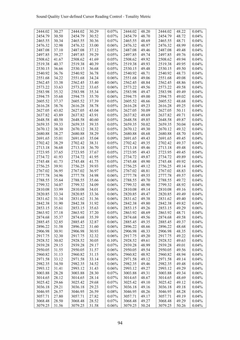
Sound Quality User-defined Cursor Reading Control - Tonality Metric
2444.02 2454.79 2465.55 2476.32 2487.08 2497.85 2508.62 2519.38 2530.15 2540.92 2551.68 2562.45 2573.22 2583.98 2594.75 2605.52 2616.28 2627.05 2637.82 2648.58 2659.35 2670.12 2680.88 2691.65 2702.42 2713.18 2723.95 2734.72 2745.48 2756.25 2767.02 2777.78 2788.55 2799.32 2810.08 2820.85 2831.62 2842.38 2853.15 2863.92 2874.68 2885.45 2896.22 2906.98 2917.75 2928.52 2939.28 2950.05 2960.82 2971.58 2982.35 2993.12 3003.88 3014.65 3025.42 3036.18 3046.95 3057.71 3068.48 3079.25
30.27 30.50 30.34 32.98 37.10 39.27 41.67 40.37 36.66 36.76 34.22 33.38 33.63 35.32 35.68 37.37 38.76 43.02 43.89 40.58 39.33 38.30 38.27 35.01 38.29 36.68 37.65 41.93 41.73 39.91 36.95 34.96 35.64 34.07 33.99 33.34 31.34 31.90 35.61 37.18 35.37 32.85 31.58 30.91 32.30 30.02 29.15 31.55 31.13 33.12 34.50 31.41 28.28 28.12 29.66 29.21 26.57 27.80 28.50 31.56
2444.02 2454.79 2465.55 2476.32 2487.08 2497.85 2508.62 2519.38 2530.15 2540.92 2551.68 2562.45 2573.22 2583.98 2594.75 2605.52 2616.28 2627.05 2637.82 2648.58 2659.35 2670.12 2680.88 2691.65 2702.42 2713.18 2723.95 2734.72 2745.48 2756.25 2767.02 2777.78 2788.55 2799.32 2810.08 2820.85 2831.62 2842.38 2853.15 2863.92 2874.68 2885.45 2896.22 2906.98 2917.75 2928.52 2939.28 2950.05 2960.82 2971.58 2982.35 2993.12 3003.88 3014.65 3025.42 3036.18 3046.95 3057.713068.48 3079.25
30.29 30.52 30.36 33.00 37.12 39.29 41.69 40.39 36.68 36.78 34.24 33.40 33.65 35.34 35.70 37.39 38.78 43.04 43.91 40.60 39.35 38.32 38.29 35.04 38.31 36.70 37.67 41.95 41.75 39.93 36.97 34.98 35.66 34.09 34.01 33.36 31.36 31.92 35.63 37.20 35.39 32.87 31.60 30.93 32.32 30.05 29.17 31.57 31.15 33.14 34.52 31.43 28.30 28.14 29.68 29.23 26.59 27.82 28.52 31.58
48.20 48.70 48.69 48.97 49.46 49.74 49.92 49.93 49.48 48.71 49.06 48.84 49.56 49.47 49.00 48.66 49.23 50.09 49.69 49.85 50.02 49.30 48.68 49.43 49.35 49.46 49.43 49.87 49.90 49.12 48.81 49.55 49.70 48.90 49.14 49.47 49.38 49.80 49.26 48.69 49.56 49.35 48.66 48.33 49.20 49.61 48.99 49.54 48.92 49.12 49.46 49.27 49.31 48.67 49.10 49.16 48.26 49.17 49.27 50.24
2444.02 2454.79 2465.55 2476.32 2487.08 2497.85 2508.62 2519.38 2530.15 2540.92 2551.68 2562.45 2573.22 2583.98 2594.752605.52 2616.28 2627.05 2637.82 2648.58 2659.35 2670.12 2680.88 2691.65 2702.42 2713.18 2723.95 2734.72 2745.48 2756.25 2767.02 2777.78 2788.55 2799.32 2810.08 2820.85 2831.62 2842.38 2853.15 2863.92 2874.68 2885.45 2896.22 2906.98 2917.75 2928.52 2939.28 2950.05 2960.82 2971.58 2982.35 2993.12 3003.88 3014.65 3025.42 3036.18 3046.95 3057.71 3068.48 3079.25
48.22 48.72 48.71 48.99 49.48 49.76 49.94 49.95 49.50 48.73 49.08 48.86 49.58 49.49 49.02 48.68 49.25 50.11 49.71 49.87 50.04 49.32 48.70 49.45 49.37 49.48 49.45 49.89 49.92 49.14 48.83 49.57 49.72 48.92 49.16 49.49 49.40 49.82 49.29 48.71 49.58 49.37 48.68 48.35 49.22 49.63 49.01 49.56 48.94 49.14 49.48 49.29 49.34 48.69 49.12 49.18 48.28 49.19 49.29 50.26
0.04% 0.04% 0.04% 0.04% 0.04% 0.04% 0.04% 0.04% 0.04% 0.04% 0.04% 0.04% 0.04% 0.04% 0.04% 0.04% 0.04% 0.04% 0.04% 0.04% 0.04% 0.04% 0.04% 0.04% 0.04% 0.04% 0.04% 0.04% 0.04% 0.04% 0.04% 0.04% 0.04% 0.04% 0.04% 0.04% 0.04% 0.04% 0.06% 0.04% 0.04% 0.04% 0.04% 0.04% 0.04% 0.04% 0.04% 0.04% 0.04% 0.04% 0.04% 0.04% 0.06% 0.04% 0.04% 0.04% 0.04% 0.04% 0.04% 0.04%
0.07% 0.07% 0.07% 0.06% 0.05% 0.05% 0.05% 0.05% 0.05%
2444.02 2454.79 2465.55 2476.32 2487.08 2497.85 2508.62 2519.38 2530.15
0.05% 2540.92 0.06% 2551.68 0.06% 2562.45 0.06% 2573.22 0.06% 2583.98 0.06% 2594.75 0.05% 2605.52 0.05% 2616.28 0.05% 2627.05 0.05% 2637.82 0.05% 2648.58 0.05% 2659.35 0.05% 2670.12 0.05% 2680.88 0.09% 2691.65 0.05% 2702.42 0.05% 2713.18 0.05% 2723.95 0.05% 2734.72 0.05% 2745.48 0.05% 2756.25 0.05% 2767.02 0.06% 2777.78 0.06% 2788.55 0.06% 2799.32 0.06% 2810.08 0.06% 2820.85 0.06% 2831.62 0.06% 2842.38 0.06% 2853.15 0.05% 2863.92 0.06% 2874.68 0.06% 2885.45 0.06% 2896.22 0.06% 2906.98 0.06% 2917.75 0.10% 2928.52 0.07% 2939.28 0.06% 2950.05 0.06% 2960.82 0.06% 2971.58
2982.35 0.06% 0.06% 2993.12
3003.88 0.07% 0.07% 3014.65
3025.42 0.07% 0.07% 3036.18 0.08% 3046.95
3057.71 0.07% 0.07% 3068.48 0.06% 3079.25
94
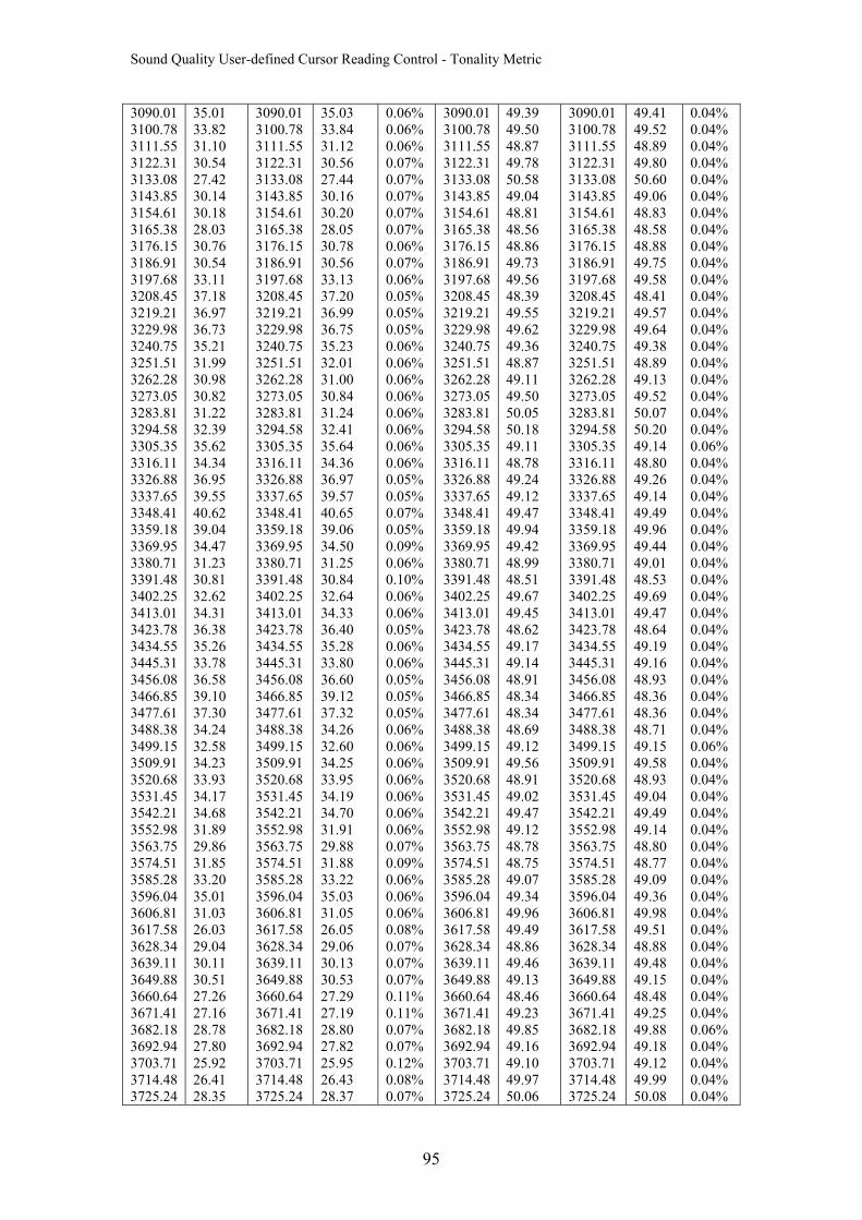
Sound Quality User-defined Cursor Reading Control - Tonality Metric
3090.01 3100.78 3111.55 3122.31 3133.08 3143.85 3154.61 3165.38 3176.15 3186.91 3197.68 3208.45 3219.21 3229.98 3240.75 3251.51 3262.28
35.01 33.82 31.10 30.54 27.42 30.14 30.18 28.03 30.76 30.54 33.11 37.18 36.97 36.73
3090.01 3100.78 3111.55 3122.31 3133.08 3143.85 3154.61 3165.38 3176.15 3186.91 3197.68 3208.45 3219.21 3229.98 3240.75 3251.51
35.03 33.84 31.12 30.56 27.44 30.16 30.20 28.05 30.78 30.56 33.13 37.20 36.99 36.75 35.23 32.01
0.06% 0.06% 0.06% 0.07% 0.07% 0.07% 0.07% 0.07% 0.06% 0.07% 0.06% 0.05% 0.05% 0.05% 0.06% 0.06% 0.06% 0.06% 0.06% 0.06%
0.06% 0.05% 0.05% 0.07% 0.05% 0.09% 0.06% 0.10% 0.06% 0.06% 0.05% 0.06% 0.06% 0.05% 0.05% 0.05% 0.06% 0.06% 0.06% 0.06% 0.06% 0.06% 0.06% 0.07% 0.09% 0.06% 0.06% 0.06% 0.08% 0.07% 0.07% 0.07% 0.11% 0.11% 0.07% 0.07% 0.12% 0.08% 0.07%
3090.01 3100.78 3111.55 3122.31 3133.08 3143.85 3154.61 3165.38 3176.15 3186.91 3197.68 3208.45 3219.21 3229.98 3240.75 3251.51 3262.28 3273.05 3283.81 3294.58 3305.35 3316.11 3326.88 3337.65 3348.41 3359.18 3369.95 3380.71 3391.48 3402.25 3413.01 3423.78 3434.55 3445.31 3456.08 3466.85 3477.61 3488.38 3499.15 3509.91 3520.68 3531.45 3542.21 3552.98 3563.75 3574.51 3585.28 3596.04 3606.81 3617.58 3628.34 3639.11 3649.88 3660.64 3671.41 3682.18 3692.94 3703.71 3714.48 3725.24
49.39 49.50 48.87 49.78 50.58 49.04 48.81 48.56 48.86 49.73 49.56 48.39 49.55 49.62 49.36 48.87 49.11 49.50 50.05 50.18 49.11 48.78 49.24 49.12 49.47 49.94 49.42 48.99 48.51 49.67 49.45 48.62 49.17 49.14 48.91 48.34 48.34 48.69 49.12 49.56 48.91 49.02 49.47 49.12 48.78 48.75 49.07 49.34 49.96 49.49 48.86 49.46 49.13 48.46 49.23 49.85 49.16 49.10 49.97 50.06
3090.01 3100.78 3111.55 3122.31 3133.08 3143.85 3154.61 3165.38 3176.15 3186.91 3197.68 3208.45 3219.21 3229.98 3240.753251.51 3262.28 3273.05 3283.81 3294.58 3305.35 3316.11 3326.88 3337.65 3348.41 3359.18 3369.95 3380.71 3391.48 3402.25 3413.01 3423.78 3434.55 3445.31 3456.08 3466.85 3477.61 3488.38 3499.15 3509.91 3520.68 3531.45 3542.21 3552.98 3563.75 3574.51 3585.28 3596.04 3606.81 3617.58 3628.34 3639.11 3649.88 3660.64 3671.41 3682.18 3692.94 3703.71 3714.48 3725.24
49.41 49.52 48.89 49.80 50.60 49.06 48.83 48.58 48.88 49.75 49.58 48.41 49.57 49.64 49.38 48.89 49.13 49.52 50.07 50.20 49.14 48.80 49.26 49.14 49.49 49.96 49.44 49.01 48.53 49.69 49.47 48.64 49.19 49.16 48.93 48.36 48.36 48.71 49.15 49.58 48.93 49.04 49.49 49.14 48.80 48.77 49.09 49.36 49.98 49.51 48.88 49.48 49.15 48.48 49.25 49.88 49.18 49.12 49.99 50.08
0.04% 0.04% 0.04% 0.04% 0.04% 0.04% 0.04% 0.04% 0.04% 0.04% 0.04% 0.04% 0.04% 0.04% 0.04% 0.04% 0.04% 0.04% 0.04% 0.04% 0.06% 0.04% 0.04% 0.04% 0.04% 0.04% 0.04% 0.04% 0.04% 0.04% 0.04% 0.04% 0.04% 0.04% 0.04% 0.04% 0.04% 0.04% 0.06% 0.04% 0.04% 0.04% 0.04% 0.04% 0.04% 0.04% 0.04% 0.04% 0.04% 0.04% 0.04% 0.04% 0.04% 0.04% 0.04% 0.06% 0.04% 0.04% 0.04% 0.04%
35.21 31.99 30.98 3262.28 31.00
3273.05 30.82 3273.05 30.84 3283.81 31.22 3283.81 31.24 3294.58 32.39 3294.58 32.41 3305.35 35.62 3305.35 35.64 0.06% 3316.11 34.34 3316.11 34.36 3326.88 36.95 3326.88 36.97 3337.65 39.55 3337.65 39.57 3348.41 40.62 3348.41 40.65 3359.18 39.04 3359.18 39.06 3369.95 34.47 3369.95 34.50 3380.71 31.23 3380.71 31.25 3391.48 30.81 3391.48 30.84 3402.25 32.62 3402.25 32.64 3413.01 34.31 3413.01 34.33 3423.78 36.38 3423.78 36.40 3434.55 35.26 3434.55 35.28 3445.31 33.78 3445.31 33.80 3456.08 36.58 3456.08 36.60 3466.85 39.10 3466.85 39.12 3477.61 37.30 3477.61 37.32 3488.38 34.24 3488.38 34.26 3499.15 32.58 3499.15 32.60 3509.91 34.23 3509.91 34.25 3520.68 33.93 3520.68 33.95 3531.45 34.17 3531.45 34.19 3542.21 34.68 3542.21 34.70 3552.98 31.89 3552.98 31.91 3563.75 29.86 3563.75 29.88 3574.51 31.85 3574.51 31.88 3585.28 33.20 3585.28 33.22 3596.04 35.01 3596.04 35.03 3606.81 31.03 3606.81 31.05 3617.58 26.03 3617.58 26.05 3628.34 29.04 3628.34 29.06 3639.11 30.11 3639.11 30.13 3649.88 30.51 3649.88 30.53 3660.64 27.26 3660.64 27.29 3671.41 27.16 3671.41 27.19 3682.18 28.78 3682.18 28.80 3692.94 27.80 3692.94 27.82 3703.71 25.92 3703.71 25.95
26.43 28.37
3714.48 26.41 3714.48 3725.24 28.35 3725.24
95
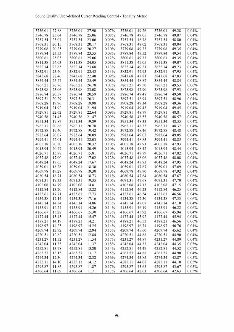
Sound Quality User-defined Cursor Reading Control - Tonality Metric
0.07% 0.08% 0.09% 0.10% 0.10% 0.08% 0.12% 0.08% 0.13% 0.13% 0.09% 0.08% 0.07% 0.09% 0.10% 0.10% 0.10% 0.09% 0.09% 0.09% 0.10% 0.10% 0.10% 0.10% 0.09% 0.10% 0.10% 0.19% 0.12% 0.11% 0.11% 0.10% 0.11% 0.10% 0.14% 0.15% 0.11% 0.12% 0.13% 0.14% 0.13% 0.13% 0.14% 0.14% 0.15% 0.16% 0.17% 0.18% 0.14% 0.15% 0.16% 0.14% 0.17% 0.17%
3736.01 3746.78 3757.54 3768.31 3779.08 3789.84 3800.61 3811.38 3822.14 3832.91 3843.68 3854.44 3865.21 3875.98 3886.74 3897.51 3908.28 3919.04 3929.81 3940.58 3951.34 3962.11 3972.88 3983.64 3994.41 4005.18 4015.94 4026.71 4037.48 4048.24 4059.01 4069.78 4080.54 4091.31 4102.08 4112.84 4123.61 4134.38 4145.14 4155.91 4166.67 4177.44 4188.21 4198.97 4209.74 4220.51 4231.27 4242.04 4252.81 4263.57 4274.34 4285.11 4295.87 4306.64
49.26 49.05 48.78 48.02 49.33 49.52 49.33 49.05 49.21 47.93 47.81 48.82 49.50 47.90 49.48 48.94 49.34 49.43 48.79 48.55 48.33 48.35 48.46 49.03 48.83 47.91 48.42 47.79 48.06 47.93 47.67 47.90 47.64 47.68 47.13 46.23 46.54 47.30 47.08 46.19 45.92 45.92 46.53 46.74 45.60 44.88 44.87 44.33 44.49 44.88 43.85 44.08 43.65 42.61
3736.01 3746.78 3757.54 3768.31 3779.08 3789.84 3800.61 3811.38 3822.14 3832.91 3843.68 3854.44 3865.21 3875.98 3886.74 3897.51 3908.28 3919.04 3929.81 3940.58 3951.34 3962.11 3972.88 3983.64 3994.41 4005.18 4015.94 4026.71 4037.48 4048.24 4059.01 4069.78 4080.54 4091.31 4102.08 4112.84 4123.61 4134.38 4145.14 4155.91 4166.67 4177.44 4188.21 4198.97 4209.74 4220.51 4231.27 4242.04 4252.81 4263.57 4274.34 4285.11 4295.87 4306.64
49.28 49.07 48.80 48.04 49.35 49.54 49.35 49.07 49.23 47.95 47.83 48.84 49.53 47.93 49.50 48.96 49.36 49.45 48.81 48.57 48.35 48.37 48.48 49.05 48.85 47.93 48.44 47.82 48.08 47.95 47.69 47.92 47.67 47.70 47.15 46.25 46.56 47.33 47.10 46.22 45.94 45.94 46.56 46.76 45.62 44.90 44.89 44.35 44.52 44.90 43.87 44.10 43.67 42.63
0.04% 0.04% 0.04% 0.04% 0.04% 0.04% 0.04% 0.04% 0.04% 0.04% 0.04% 0.04% 0.06% 0.06% 0.04% 0.04% 0.04% 0.04% 0.04% 0.04% 0.04% 0.04% 0.04% 0.04% 0.04% 0.04% 0.04% 0.06% 0.04% 0.04% 0.04% 0.04% 0.06% 0.04% 0.04% 0.04% 0.04% 0.06% 0.04% 0.06% 0.04% 0.04% 0.06% 0.04% 0.04% 0.04% 0.04% 0.05% 0.07% 0.04% 0.05% 0.05% 0.05% 0.05%
27.90 25.06 23.06
20.27 23.55 25.06 24.05 23.68
22.48 25.49 26.78 23.08 20.59
19.98 21.94 22.64 21.47 19.89
19.42 20.09 22.03 20.32 20.49
17.02 17.67 18.30 19.30 18.73
14.81 13.22 17.73 17.16 14.86
15.30 15.47 14.21 14.25 12.94
11.54 11.37 13.80 13.17 12.32
11.87 11.71
3736.01 27.88 3736.01 3746.78 25.04 3746.78 3757.54 23.04 3757.54
20.17 3768.31 20.15 3768.31 3779.08 20.25 3779.08 3789.84 23.53 3789.84 3800.61 25.03 3800.61 3811.38 24.03 3811.38 3822.14 23.65 3822.14
23.43 3832.91 23.40 3832.91 3843.68 22.46 3843.68 3854.44 25.47 3854.44 3865.21 26.76 3865.21 3875.98 23.06 3875.98 3886.74 20.57 3886.74
20.31 3897.51 20.29 3897.51 3908.28 19.96 3908.28 3919.04 21.92 3919.04 3929.81 22.62 3929.81 3940.58 21.45 3940.58 3951.34 19.87 3951.34
20.70 3962.11 20.68 3962.11 3972.88 19.40 3972.88 3983.64 20.07 3983.64 3994.41 22.01 3994.41 4005.18 20.30 4005.18 4015.94 20.47 4015.94
15.81 4026.71 15.78 4026.71 4037.48 17.00 4037.48 4048.24 17.65 4048.24 4059.01 18.28 4059.01 4069.78 19.28 4069.78 4080.54 18.71 4080.54
19.35 4091.31 19.33 4091.31 4102.08 14.79 4102.08 4112.84 13.20 4112.84 4123.61 17.71 4123.61 4134.38 17.14 4134.38 4145.14 14.84 4145.14
14.26 4155.91 14.24 4155.91 4166.67 15.28 4166.67 4177.44 15.45 4177.44 4188.21 14.19 4188.21 4198.97 14.23 4198.97 4209.74 12.92 4209.74
12.84 4220.51 12.82 4220.51 4231.27 11.52 4231.27 4242.04 11.35 4242.04 4252.81 13.78 4252.81 4263.57 13.15 4263.57 4274.34 12.30 4274.34
14.12 4285.11 14.10 4285.11 4295.87 11.85 4295.87 4306.64 11.69 4306.64
96

Sound Quality User-defined Cursor Reading Control - Tonality Metric
Appendix D MATLAB Source Code for Stationary Loudness
97
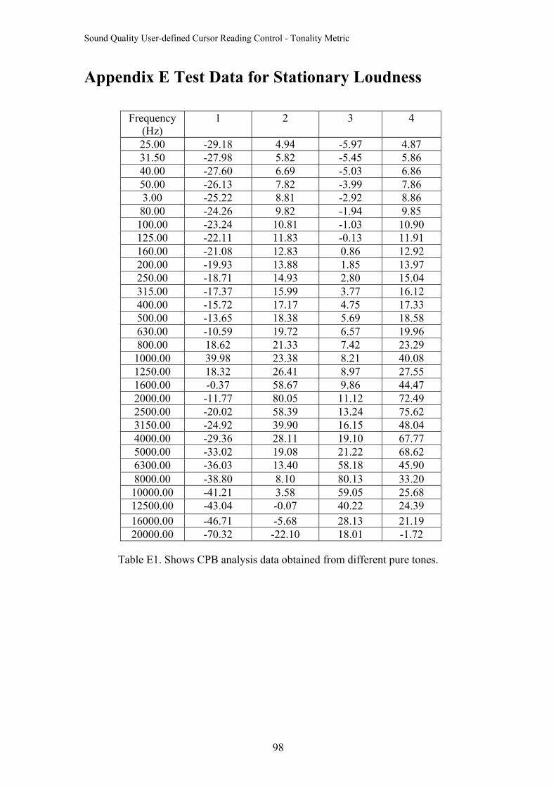
Sound Quality User-defined Cursor Reading Control - Tonality Metric
Appendix E Test Data for Stationary Loudness
Frequency
(Hz) 1 2 3 4
25.00 -29.18 4.94 -5.97 4.87 31.50 -27.98 5.82 -5.45 5.86 40.00 -27.60 6.69 -5.03 6.86 50.00 -26.13 7.82 -3.99 7.86 3.00 -25.22 8.81 -2.92 8.86 80.00 -24.26 9.82 -1.94 9.85 100.00 -23.24 10.81 -1.03 10.90 125.00 -22.11 11.83 -0.13 11.91 160.00 -21.08 12.83 0.86 12.92 200.00 -19.93 13.88 1.85 13.97 250.00 -18.71 14.93 2.80 15.04 315.00 -17.37 15.99 3.77 16.12 400.00 -15.72 17.17 4.75 17.33 500.00 -13.65 18.38 5.69 18.58 630.00 -10.59 19.72 6.57 19.96 800.00 18.62 21.33 7.42 23.29 1000.00 39.98 23.38 8.21 40.08 1250.00 18.32 26.41 8.97 27.55 1600.00 -0.37 58.67 9.86 44.47 2000.00 -11.77 80.05 11.12 72.49 2500.00 -20.02 58.39 13.24 75.62 3150.00 -24.92 39.90 16.15 48.04 4000.00 -29.36 28.11 19.10 67.77 5000.00 -33.02 19.08 21.22 68.62 6300.00 -36.03 13.40 58.18 45.90 8000.00 -38.80 8.10 80.13 33.20 10000.00 -41.21 3.58 59.05 25.68 12500.00 -43.04 -0.07 40.22 24.39 16000.00 -46.71 -5.68 28.13 21.19 20000.00 -70.32 -22.10 18.01 -1.72
Table E1. Shows CPB analysis data obtained from different pure tones.
98
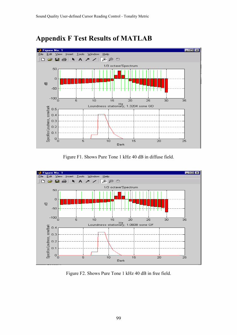
Sound Quality User-defined Cursor Reading Control - Tonality Metric
Appendix F Test Results of MATLAB
Figure F1. Shows Pure Tone 1 kHz 40 dB in diffuse field.
Figure F2. Shows Pure Tone 1 kHz 40 dB in free field.
99
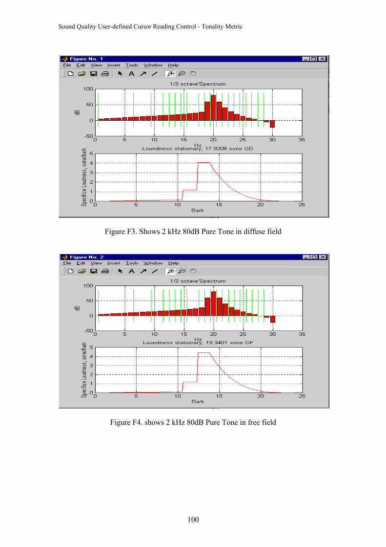
Sound Quality User-defined Cursor Reading Control - Tonality Metric
Figure F3. Shows 2 kHz 80dB Pure Tone in diffuse field
Figure F4. shows 2 kHz 80dB Pure Tone in free field
100
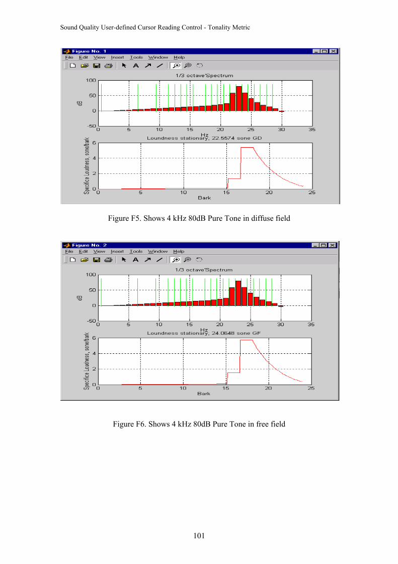
Sound Quality User-defined Cursor Reading Control - Tonality Metric
Figure F5. Shows 4 kHz 80dB Pure Tone in diffuse field
Figure F6. Shows 4 kHz 80dB Pure Tone in free field
101
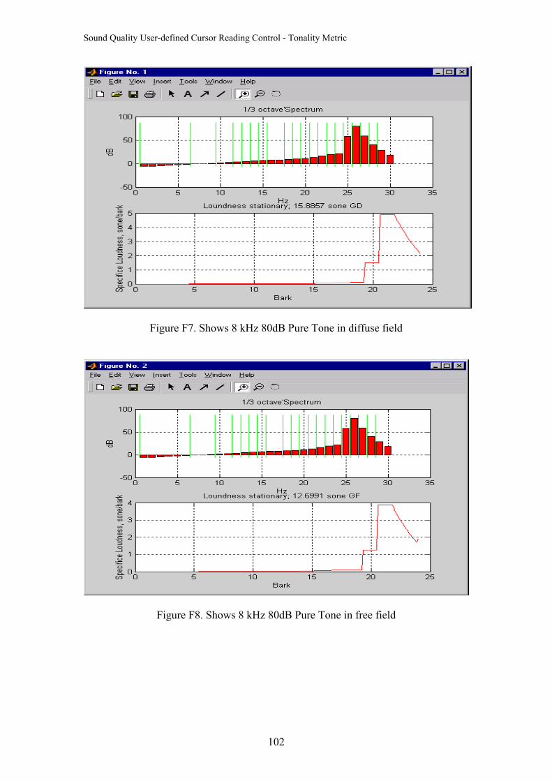
Sound Quality User-defined Cursor Reading Control - Tonality Metric
Figure F7. Shows 8 kHz 80dB Pure Tone in diffuse field
Figure F8. Shows 8 kHz 80dB Pure Tone in free field
102

Sound Quality User-defined Cursor Reading Control - Tonality Metric
Appendix G Algorithm for Extraction of Pitch and Pitch Salience from Complex Tonal Signals
103

Sound Quality User-defined Cursor Reading Control - Tonality Metric
Appendix H Pitch of Complex Signals according to Virtual-pitch Theory: Tests, examples, and predictions.
104

Sound Quality User-defined Cursor Reading Control - Tonality Metric
Appendix I International Standard ISO 532 Acoustics – Method for Calculating Loudness Level
105

Sound Quality User-defined Cursor Reading Control - Tonality Metric
Appendix J DIN 45 631 - Procedure for Calculating Loudness Level and Loudness
106

Sound Quality User-defined Cursor Reading Control - Tonality Metric
Appendix K An Examination of Aures’s Model of Tonality
107

Sound Quality User-defined Cursor Reading Control - Tonality Metric
Appendix L Lecture Notes ‘Introduction to Sound Quality’ by B&K A/S
108

Sound Quality User-defined Cursor Reading Control - Tonality Metric
Appendix M Lecture Notes ‘Psychoacoustics – A Qualitative Description’ by B&K A/S
109
Filename: Tonality_Final_Thesis Directory: E:\ThesisCD Template: C:\Documents and Settings\fkc\Application
Data\Microsoft\Templates\Normal.dot Title: Sound Quality User-defined Cursor Reading Control Subject: Author: zzhong Keywords: Comments: Creation Date: 09-03-2003 16:17 Change Number: 4 Last Saved On: 09-03-2003 16:45 Last Saved By: zzhong Total Editing Time: 13 Minutes Last Printed On: 11-03-2003 11:16 As of Last Complete Printing Number of Pages: 110 Number of Words: 28.621 (approx.) Number of Characters: 163.145 (approx.)