Embed Size (px)
Citation preview
Last Updated: 12-03-13 11:11 AM CSE 2011 Prof. J. Elder - 1 -
Sorting
Chapter 11
Last Updated: 12-03-13 11:11 AM CSE 2011 Prof. J. Elder - 2 -
Sorting
Ø We have seen the advantage of sorted data representations for a number of applications q Sparse vectors
q Maps
q Dictionaries
Ø Here we consider the problem of how to efficiently transform an unsorted representation into a sorted representation.
Ø We will focus on sorted array representations.

Last Updated: 12-03-13 11:11 AM CSE 2011 Prof. J. Elder - 3 -
Sorting Algorithms Ø Comparison Sorting
q Selection Sort
q Bubble Sort
q Insertion Sort
q Merge Sort
q Heap Sort
q Quick Sort
Ø Linear Sorting q Counting Sort
q Radix Sort
q Bucket Sort
Last Updated: 12-03-13 11:11 AM CSE 2011 Prof. J. Elder - 4 -
Comparison Sorts
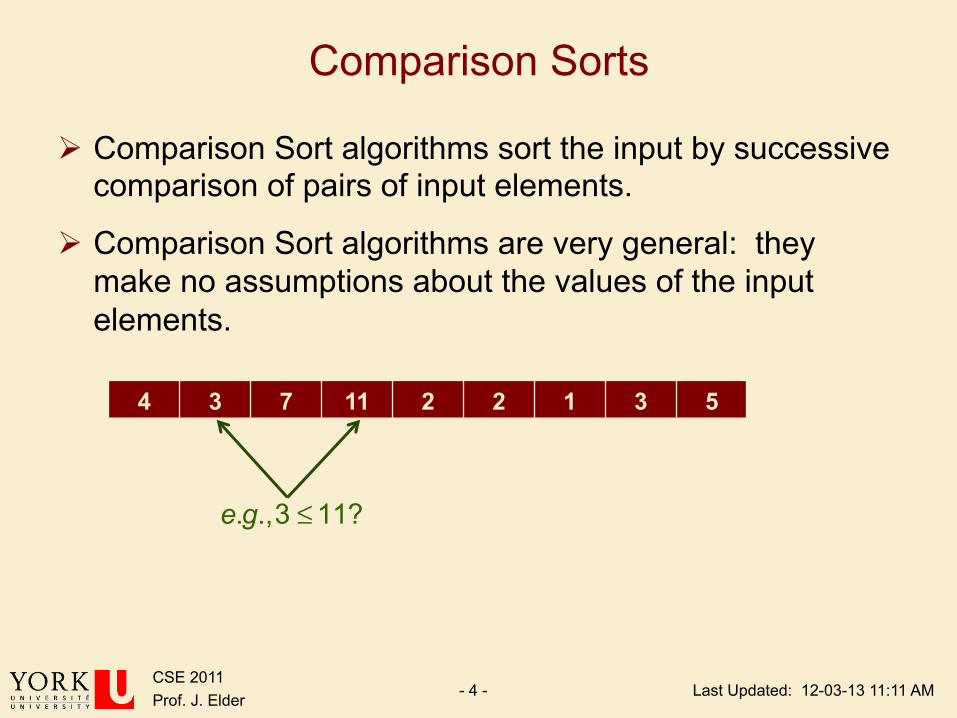
Ø Comparison Sort algorithms sort the input by successive comparison of pairs of input elements.
Ø Comparison Sort algorithms are very general: they make no assumptions about the values of the input elements.
4 3 7 11 2 2 1 3 5
e.g.,3 !11?
Last Updated: 12-03-13 11:11 AM CSE 2011 Prof. J. Elder - 5 -
Sorting Algorithms and Memory
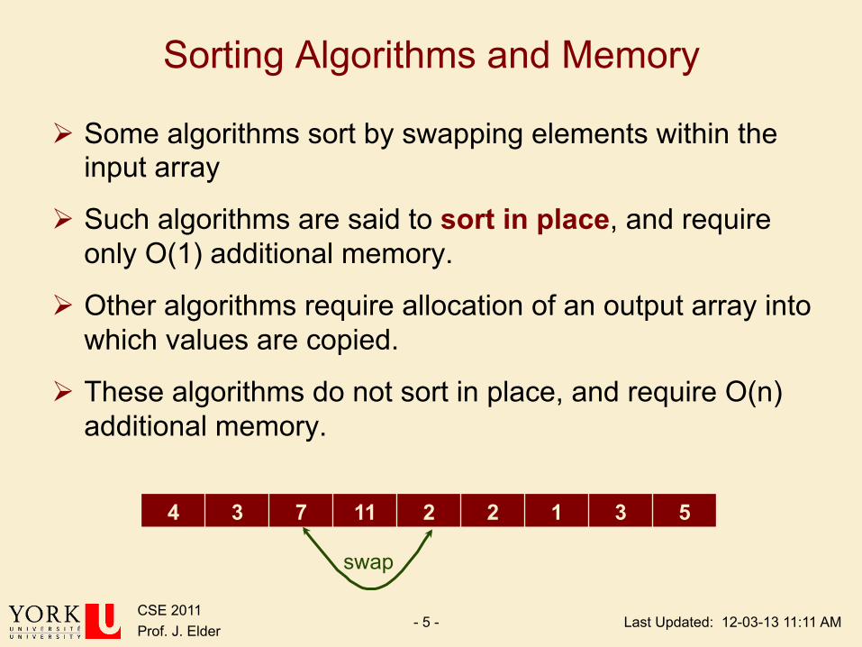
Ø Some algorithms sort by swapping elements within the input array
Ø Such algorithms are said to sort in place, and require only O(1) additional memory.
Ø Other algorithms require allocation of an output array into which values are copied.
Ø These algorithms do not sort in place, and require O(n) additional memory.
4 3 7 11 2 2 1 3 5
swap
Last Updated: 12-03-13 11:11 AM CSE 2011 Prof. J. Elder - 6 -
Stable Sort
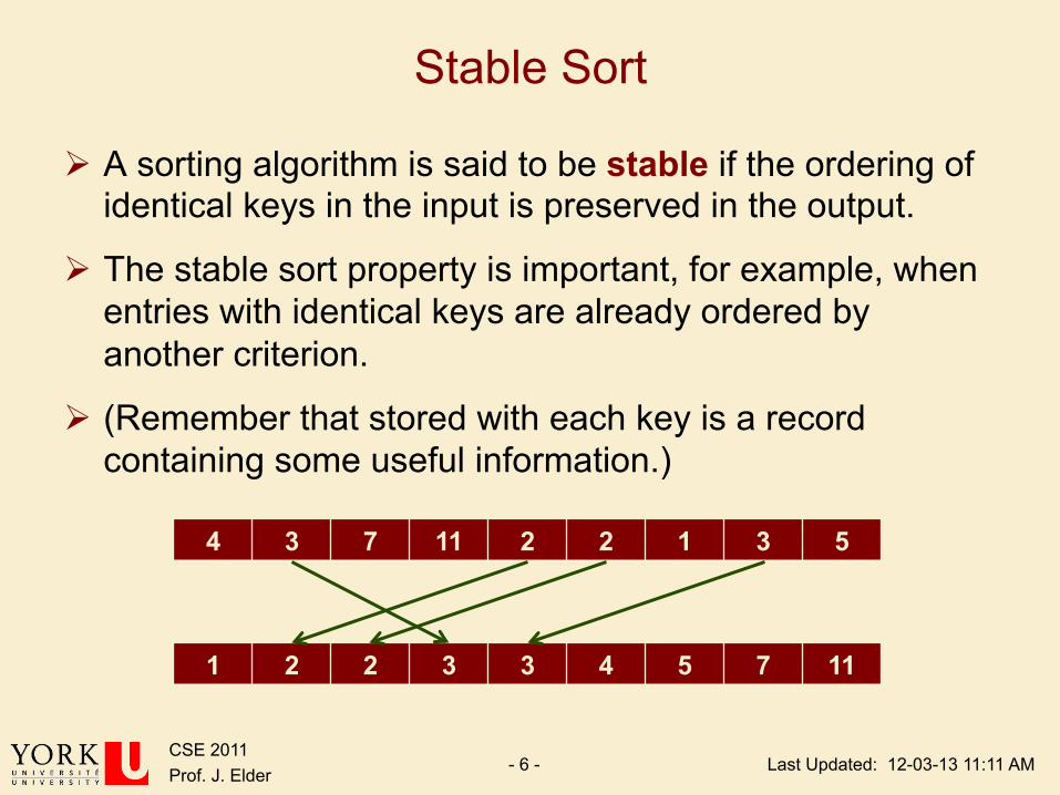
Ø A sorting algorithm is said to be stable if the ordering of identical keys in the input is preserved in the output.
Ø The stable sort property is important, for example, when entries with identical keys are already ordered by another criterion.
Ø (Remember that stored with each key is a record containing some useful information.)
4 3 7 11 2 2 1 3 5
1 2 2 3 3 4 5 7 11
Last Updated: 12-03-13 11:11 AM CSE 2011 Prof. J. Elder - 7 -
Selection Sort
Ø Selection Sort operates by first finding the smallest element in the input list, and moving it to the output list.
Ø It then finds the next smallest value and does the same.
Ø It continues in this way until all the input elements have been selected and placed in the output list in the correct order.
Ø Note that every selection requires a search through the input list.
Ø Thus the algorithm has a nested loop structure
Ø Selection Sort Example
Last Updated: 12-03-13 11:11 AM CSE 2011 Prof. J. Elder - 8 -
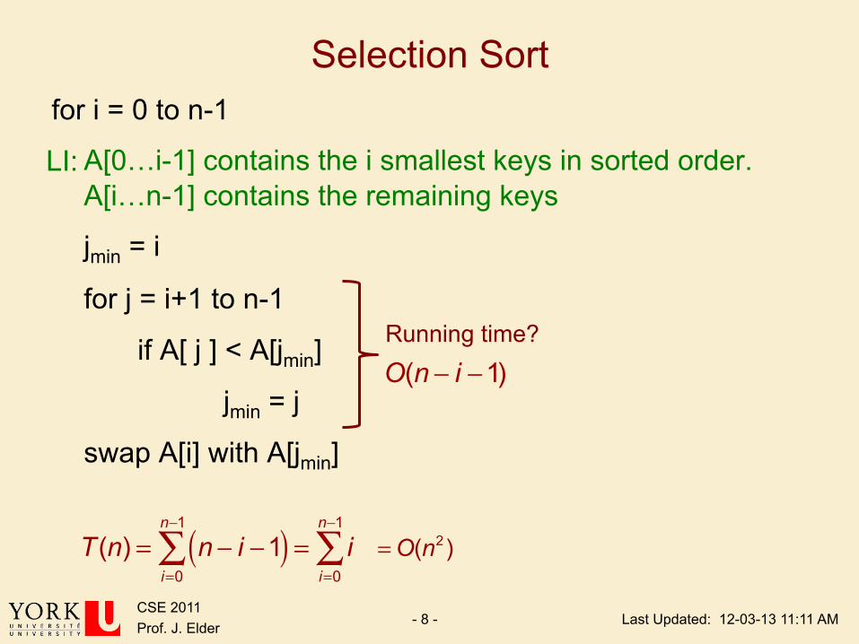
Selection Sort for i = 0 to n-1
A[0…i-1] contains the i smallest keys in sorted order. A[i…n-1] contains the remaining keys
jmin = i
for j = i+1 to n-1
if A[ j ] < A[jmin]
jmin = j
swap A[i] with A[jmin]
O(n ! i !1)
T(n) = n ! i !1( )
i=0
n!1
" = ii=0
n!1
" = O(n2)
Running time?
LI:
Last Updated: 12-03-13 11:11 AM CSE 2011 Prof. J. Elder - 9 -
Bubble Sort
Ø Bubble Sort operates by successively comparing adjacent elements, swapping them if they are out of order.
Ø At the end of the first pass, the largest element is in the correct position.
Ø A total of n passes are required to sort the entire array.
Ø Thus bubble sort also has a nested loop structure
Ø Bubble Sort Example

Last Updated: 12-03-13 11:11 AM CSE 2011 Prof. J. Elder - 10 -
Expert Opinion on Bubble Sort
Last Updated: 12-03-13 11:11 AM CSE 2011 Prof. J. Elder - 11 -
Bubble Sort
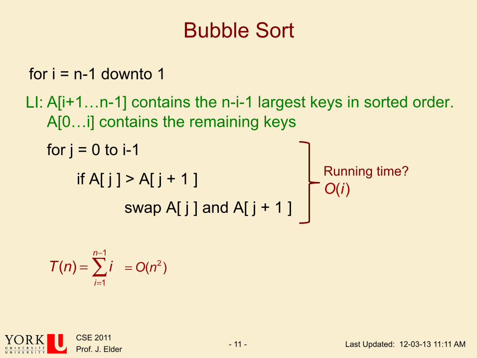
for i = n-1 downto 1
A[i+1…n-1] contains the n-i-1 largest keys in sorted order. A[0…i] contains the remaining keys
for j = 0 to i-1
if A[ j ] > A[ j + 1 ]
swap A[ j ] and A[ j + 1 ]
O(i)
T(n) = i
i=1
n!1
" = O(n2)
Running time?
LI:
Last Updated: 12-03-13 11:11 AM CSE 2011 Prof. J. Elder - 12 -
Comparison
Ø Thus both Selection Sort and Bubble Sort have O(n2) running time.
Ø However, both can also easily be designed to q Sort in place
q Stable sort
Last Updated: 12-03-13 11:11 AM CSE 2011 Prof. J. Elder - 13 -
Insertion Sort
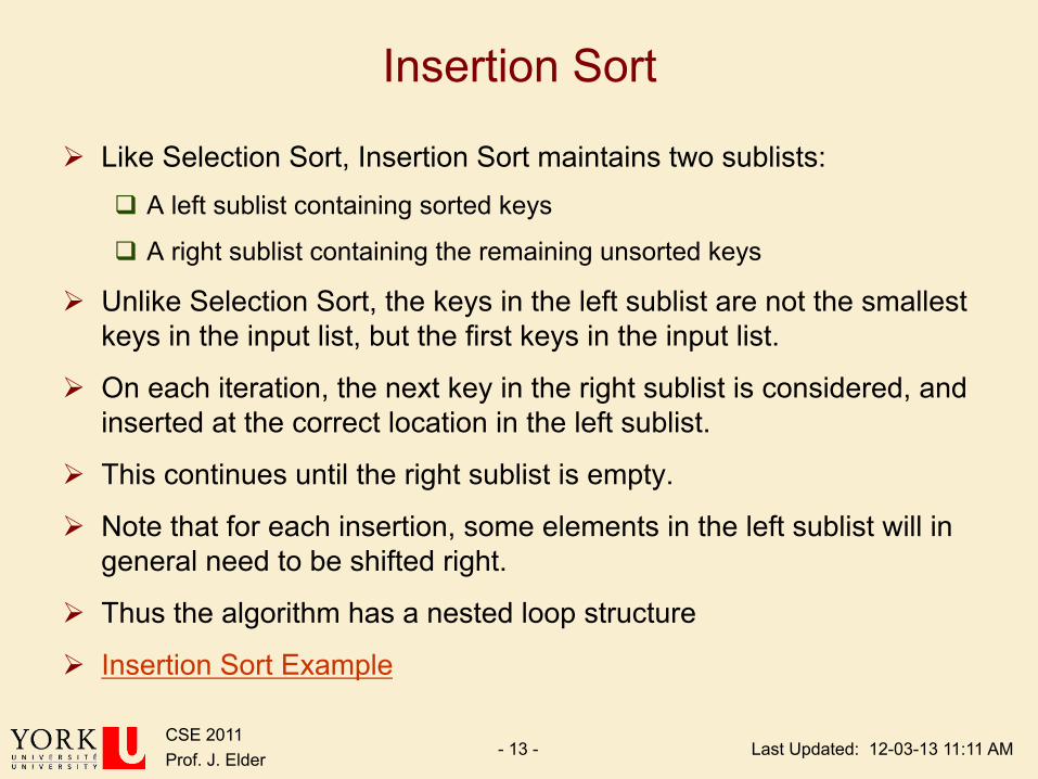
Ø Like Selection Sort, Insertion Sort maintains two sublists: q A left sublist containing sorted keys
q A right sublist containing the remaining unsorted keys
Ø Unlike Selection Sort, the keys in the left sublist are not the smallest keys in the input list, but the first keys in the input list.
Ø On each iteration, the next key in the right sublist is considered, and inserted at the correct location in the left sublist.
Ø This continues until the right sublist is empty.
Ø Note that for each insertion, some elements in the left sublist will in general need to be shifted right.
Ø Thus the algorithm has a nested loop structure
Ø Insertion Sort Example
Last Updated: 12-03-13 11:11 AM CSE 2011 Prof. J. Elder - 14 -
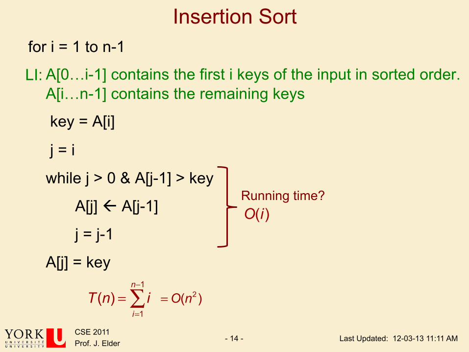
Insertion Sort for i = 1 to n-1
A[0…i-1] contains the first i keys of the input in sorted order. A[i…n-1] contains the remaining keys
key = A[i]
j = i
while j > 0 & A[j-1] > key
A[j] ß A[j-1]
j = j-1
A[j] = key
O(i)
T(n) = i
i=1
n!1
" = O(n2)
Running time?
LI:
Last Updated: 12-03-13 11:11 AM CSE 2011 Prof. J. Elder - 15 -
Comparison
Ø Selection Sort
Ø Bubble Sort
Ø Insertion Sort q Sort in place
q Stable sort
q But O(n2) running time.
Ø Can we do better?
Last Updated: 12-03-13 11:11 AM CSE 2011 Prof. J. Elder - 16 -
Divide-and-Conquer
Ø Divide-and conquer is a general algorithm design paradigm: q Divide: divide the input data S in two disjoint subsets S1 and S2
q Recur: solve the subproblems associated with S1 and S2
q Conquer: combine the solutions for S1 and S2 into a solution for S
Ø The base case for the recursion is a subproblem of size 0 or 1
Last Updated: 12-03-13 11:11 AM CSE 2011 Prof. J. Elder - 17 -
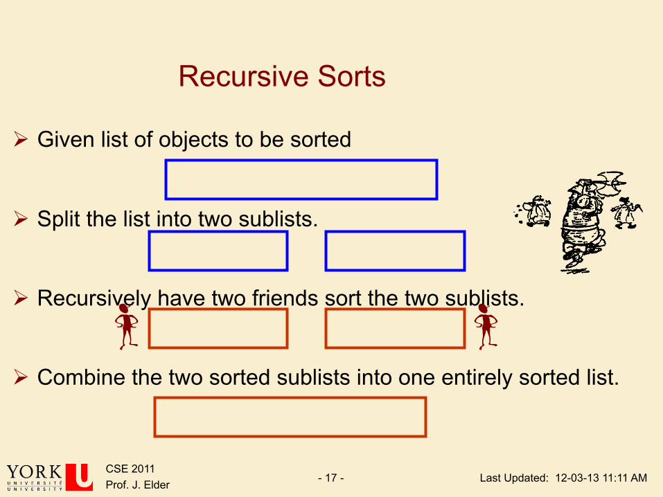
Recursive Sorts
Ø Given list of objects to be sorted
Ø Split the list into two sublists.
Ø Recursively have two friends sort the two sublists.
Ø Combine the two sorted sublists into one entirely sorted list.

Last Updated: 12-03-13 11:11 AM CSE 2011 Prof. J. Elder - 18 -
Merge Sort
88 14 98 25
62
52
79
30 23
31
Divide and Conquer

Last Updated: 12-03-13 11:11 AM CSE 2011 Prof. J. Elder - 19 -
Merge Sort
Ø Merge-sort is a sorting algorithm based on the divide-and-conquer paradigm
Ø It was invented by John von Neumann, one of the pioneers of computing, in 1945
Last Updated: 12-03-13 11:11 AM CSE 2011 Prof. J. Elder - 20 -
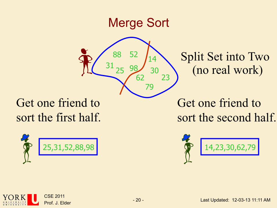
Merge Sort
88 14 98 25
62
52
79
30 23
31 Split Set into Two
(no real work)
25,31,52,88,98
Get one friend to sort the first half.
14,23,30,62,79
Get one friend to sort the second half.
Last Updated: 12-03-13 11:11 AM CSE 2011 Prof. J. Elder - 21 -
Merge Sort
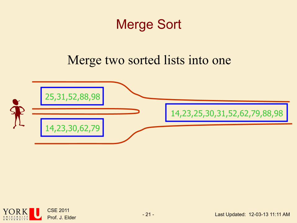
Merge two sorted lists into one
25,31,52,88,98
14,23,30,62,79
14,23,25,30,31,52,62,79,88,98
Last Updated: 12-03-13 11:11 AM CSE 2011 Prof. J. Elder - 22 -
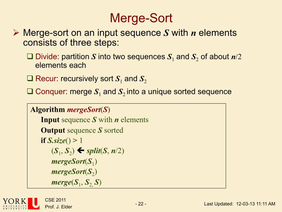
Merge-Sort Ø Merge-sort on an input sequence S with n elements
consists of three steps: q Divide: partition S into two sequences S1 and S2 of about n/2
elements each
q Recur: recursively sort S1 and S2
q Conquer: merge S1 and S2 into a unique sorted sequence
Algorithm mergeSort(S) Input sequence S with n elements Output sequence S sorted if S.size() > 1
(S1, S2) ç split(S, n/2) mergeSort(S1) mergeSort(S2) merge(S1, S2, S)
Last Updated: 12-03-13 11:11 AM CSE 2011 Prof. J. Elder - 23 -
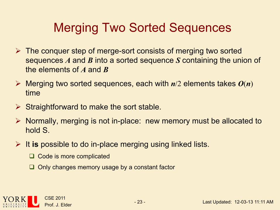
Merging Two Sorted Sequences
Ø The conquer step of merge-sort consists of merging two sorted sequences A and B into a sorted sequence S containing the union of the elements of A and B
Ø Merging two sorted sequences, each with n/2 elements takes O(n) time
Ø Straightforward to make the sort stable.
Ø Normally, merging is not in-place: new memory must be allocated to hold S.
Ø It is possible to do in-place merging using linked lists. q Code is more complicated
q Only changes memory usage by a constant factor
Last Updated: 12-03-13 11:11 AM CSE 2011 Prof. J. Elder - 24 -
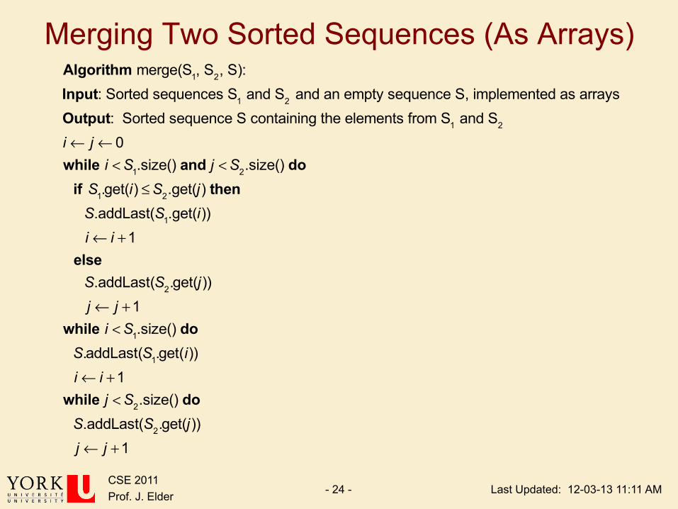
Merging Two Sorted Sequences (As Arrays)
Algorithm merge(S1, S2, S):
Input: Sorted sequences S1 and S2 and an empty sequence S, implemented as arrays
Output: Sorted sequence S containing the elements from S1 and S2
i ! j ! 0while i <S1.size() and j <S2.size() do
if S1.get(i) "S2.get(j) thenS.addLast(S1.get(i))i ! i +1
elseS.addLast(S2.get(j))j ! j +1
while i <S1.size() doS.addLast(S1.get(i))i ! i +1
while j <S2.size() doS.addLast(S2.get(j))j ! j +1
Last Updated: 12-03-13 11:11 AM CSE 2011 Prof. J. Elder - 25 -
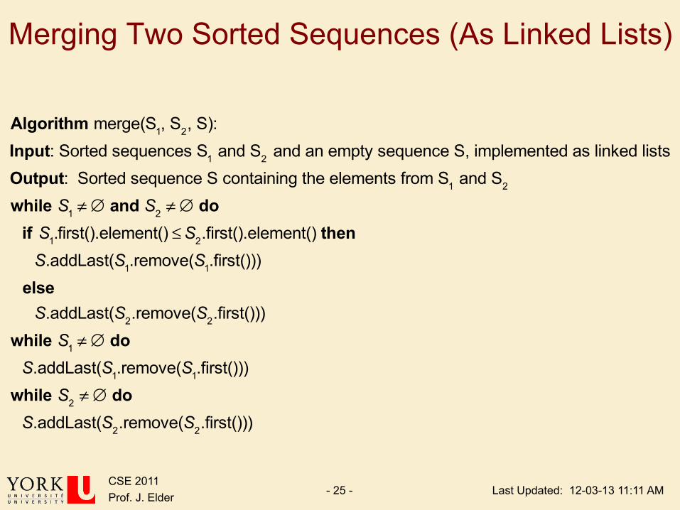
Merging Two Sorted Sequences (As Linked Lists)
Algorithm merge(S1, S2, S):
Input: Sorted sequences S1 and S2 and an empty sequence S, implemented as linked lists
Output: Sorted sequence S containing the elements from S1 and S2
while S1 ! " and S2 ! " doif S1.first().element() #S2.first().element() then
S.addLast(S1.remove(S1.first()))
elseS.addLast(S2.remove(S2.first()))
while S1 ! " doS.addLast(S1.remove(S1.first()))
while S2 ! " doS.addLast(S2.remove(S2.first()))
Last Updated: 12-03-13 11:11 AM CSE 2011 Prof. J. Elder - 26 -
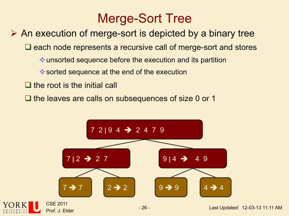
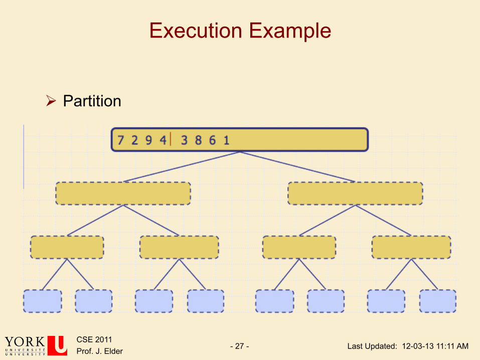
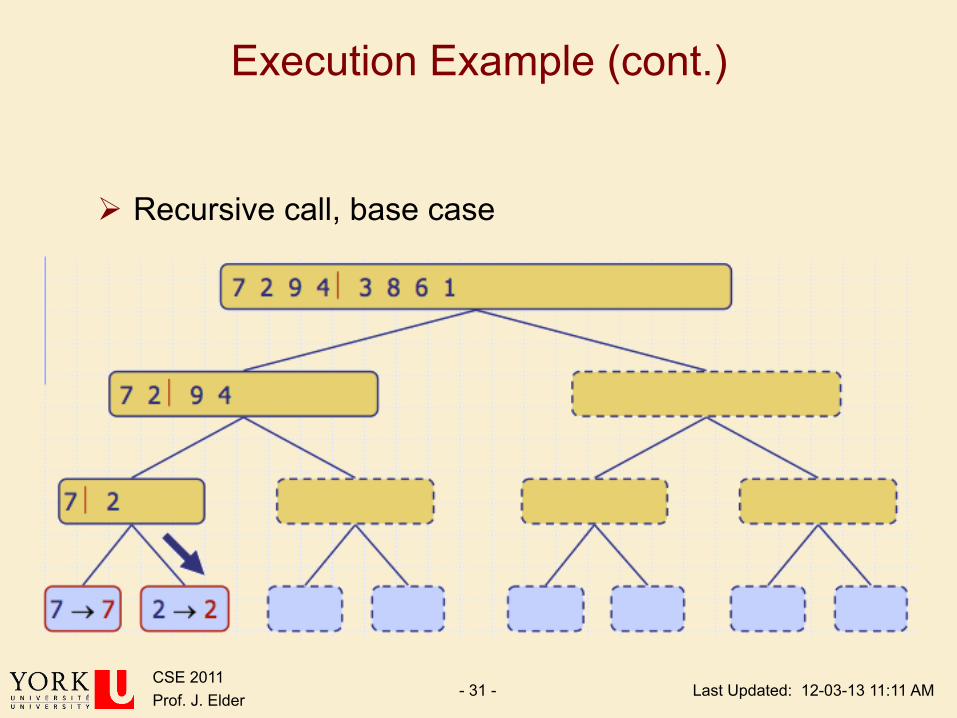
Merge-Sort Tree Ø An execution of merge-sort is depicted by a binary tree
q each node represents a recursive call of merge-sort and stores ² unsorted sequence before the execution and its partition
² sorted sequence at the end of the execution
q the root is the initial call q the leaves are calls on subsequences of size 0 or 1
7 2 | 9 4 è 2 4 7 9
7 | 2 è 2 7 9 | 4 è 4 9
7 è 7 2 è 2 9 è 9 4 è 4
Last Updated: 12-03-13 11:11 AM CSE 2011 Prof. J. Elder - 27 -
Execution Example
Ø Partition
Last Updated: 12-03-13 11:11 AM CSE 2011 Prof. J. Elder - 28 -
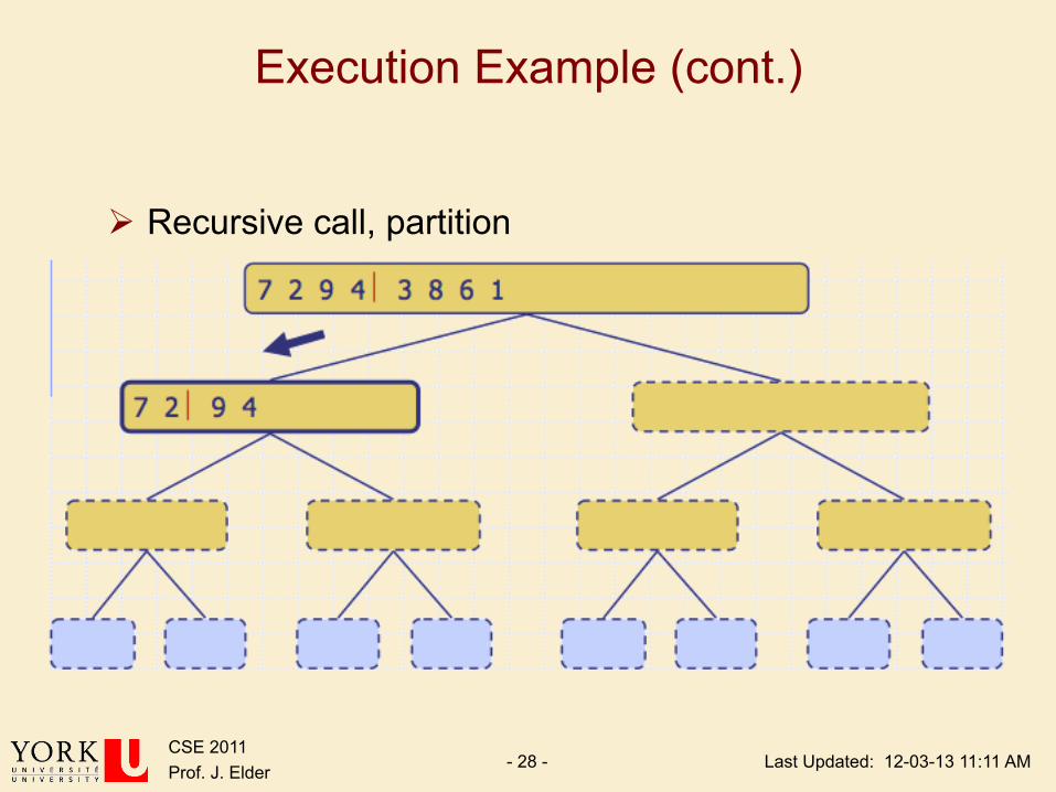
Execution Example (cont.)
Ø Recursive call, partition
Last Updated: 12-03-13 11:11 AM CSE 2011 Prof. J. Elder - 29 -
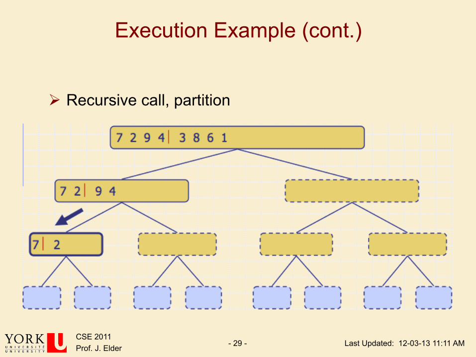
Execution Example (cont.)
Ø Recursive call, partition
Last Updated: 12-03-13 11:11 AM CSE 2011 Prof. J. Elder - 30 -
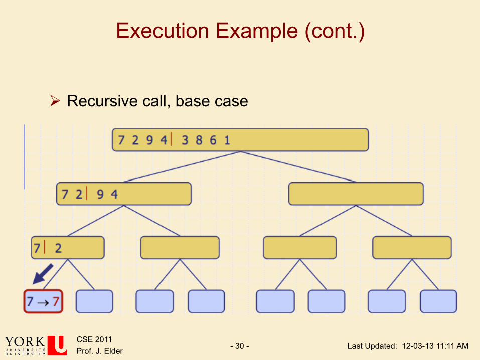
Execution Example (cont.)
Ø Recursive call, base case
Last Updated: 12-03-13 11:11 AM CSE 2011 Prof. J. Elder - 31 -
Execution Example (cont.)
Ø Recursive call, base case

Last Updated: 12-03-13 11:11 AM CSE 2011 Prof. J. Elder - 32 -
Execution Example (cont.)
Ø Merge
Last Updated: 12-03-13 11:11 AM CSE 2011 Prof. J. Elder - 33 -
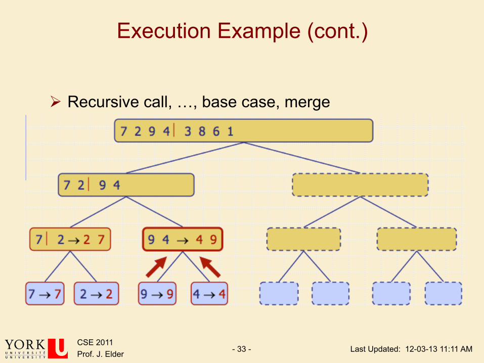
Execution Example (cont.)
Ø Recursive call, …, base case, merge

Last Updated: 12-03-13 11:11 AM CSE 2011 Prof. J. Elder - 34 -
Execution Example (cont.)
Ø Merge

Last Updated: 12-03-13 11:11 AM CSE 2011 Prof. J. Elder - 35 -
Execution Example (cont.)
Ø Recursive call, …, merge, merge

Last Updated: 12-03-13 11:11 AM CSE 2011 Prof. J. Elder - 36 -
Execution Example (cont.)
Ø Merge

Last Updated: 12-03-13 11:11 AM CSE 2011 Prof. J. Elder - 37 -
End of Lecture
March 11, 2012
Last Updated: 12-03-13 11:11 AM CSE 2011 Prof. J. Elder - 38 -
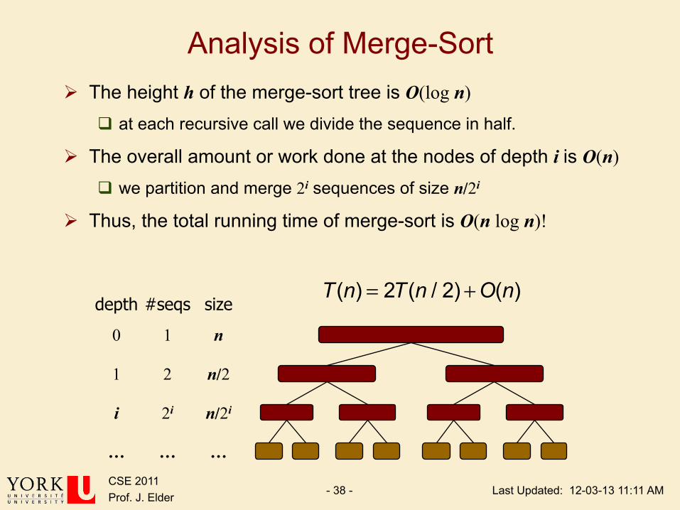
Analysis of Merge-Sort Ø The height h of the merge-sort tree is O(log n)
q at each recursive call we divide the sequence in half.
Ø The overall amount or work done at the nodes of depth i is O(n) q we partition and merge 2i sequences of size n/2i
Ø Thus, the total running time of merge-sort is O(n log n)!
depth #seqs size
0 1 n
1 2 n/2
i 2i n/2i
… … …
T(n) = 2T(n / 2) +O(n)

Last Updated: 12-03-13 11:11 AM CSE 2011 Prof. J. Elder - 39 -
Running Time of Comparison Sorts
Ø Thus MergeSort is much more efficient than SelectionSort, BubbleSort and InsertionSort. Why?
Ø You might think that to sort n keys, each key would have to at some point be compared to every other key:
Ø However, this is not the case. q Transitivity: If A < B and B < C, then you know that A < C, even
though you have never directly compared A and C.
q MergeSort takes advantage of this transitivity property in the merge stage.
!O n2( )
Last Updated: 12-03-13 11:11 AM CSE 2011 Prof. J. Elder - 40 -
Heapsort
Ø Invented by Williams & Floyd in 1964
Ø O(nlogn) worst case – like merge sort
Ø Sorts in place – like selection sort
Ø Combines the best of both algorithms
Last Updated: 12-03-13 11:11 AM CSE 2011 Prof. J. Elder - 41 -
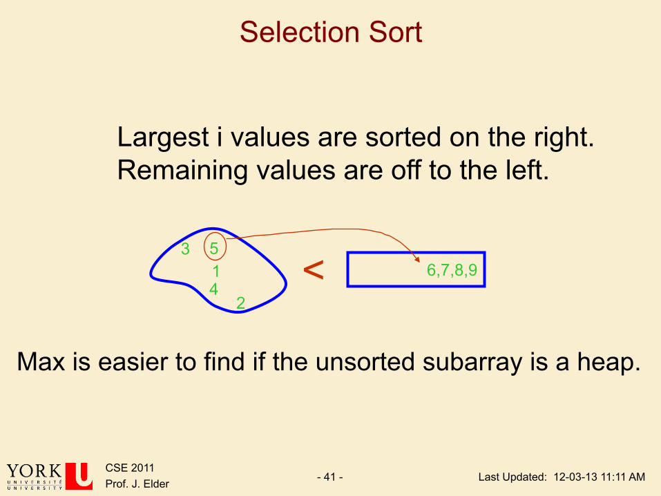
Selection Sort
Largest i values are sorted on the right. Remaining values are off to the left.
6,7,8,9 < 3
4 1 5
2
Max is easier to find if the unsorted subarray is a heap.
Last Updated: 12-03-13 11:11 AM CSE 2011 Prof. J. Elder - 42 -
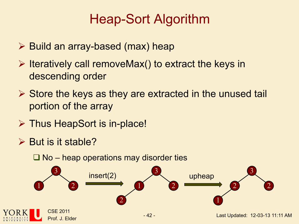
Heap-Sort Algorithm
Ø Build an array-based (max) heap
Ø Iteratively call removeMax() to extract the keys in descending order
Ø Store the keys as they are extracted in the unused tail portion of the array
Ø Thus HeapSort is in-place!
Ø But is it stable? q No – heap operations may disorder ties
3
2 1
3
2 1
2
3
2 2
1
insert(2) upheap
Last Updated: 12-03-13 11:11 AM CSE 2011 Prof. J. Elder - 43 -
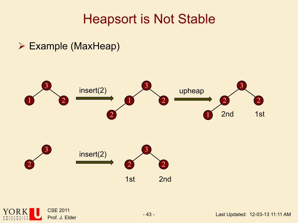
Heapsort is Not Stable
Ø Example (MaxHeap)
3
2 1
3
2 1
2
3
2 2
1
insert(2) upheap
3
2 insert(2)
1st 2nd
3
2 2
1st 2nd
Last Updated: 12-03-13 11:11 AM CSE 2011 Prof. J. Elder - 44 -
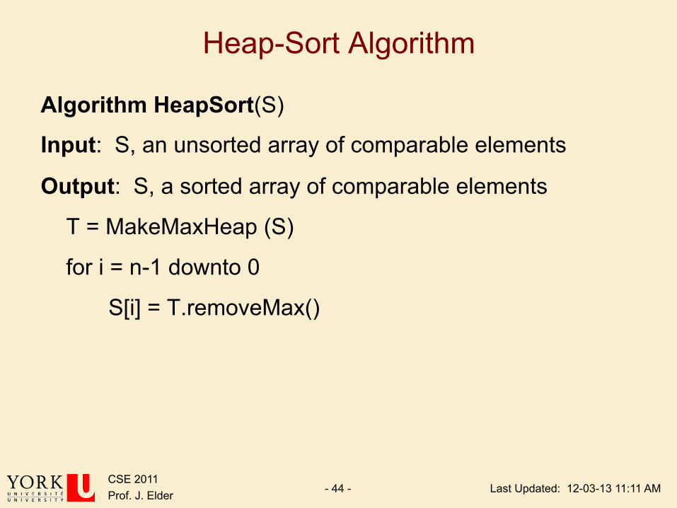
Heap-Sort Algorithm
Algorithm HeapSort(S)
Input: S, an unsorted array of comparable elements
Output: S, a sorted array of comparable elements
T = MakeMaxHeap (S)
for i = n-1 downto 0
S[i] = T.removeMax()
Last Updated: 12-03-13 11:11 AM CSE 2011 Prof. J. Elder - 45 -
Heap Sort Example (Using Min Heap)

Last Updated: 12-03-13 11:11 AM CSE 2011 Prof. J. Elder - 46 -
Heap-Sort Running Time
Ø The heap can be built bottom-up in O(n) time
Ø Extraction of the ith element takes O(log(n - i+1)) time (for downheaping)
Ø Thus total run time is
T(n) = O(n) + log(n ! i +1)i=1
n
"
= O(n) + log ii=1
n
"
#O(n) + logni=1
n
"= O(n logn)
Last Updated: 12-03-13 11:11 AM CSE 2011 Prof. J. Elder - 47 -
Heap-Sort Running Time
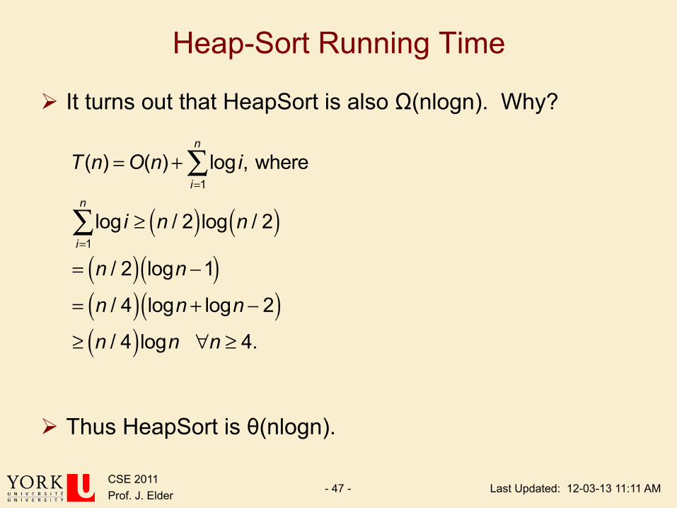
Ø It turns out that HeapSort is also Ω(nlogn). Why?
Ø Thus HeapSort is θ(nlogn).
T(n) = O(n)+ log ii=1
n
! , where
log ii=1
n
! " n / 2( )log n / 2( )= n / 2( ) logn #1( )= n / 4( ) logn + logn # 2( )" n / 4( )logn $n " 4.
Last Updated: 12-03-13 11:11 AM CSE 2011 Prof. J. Elder - 48 -
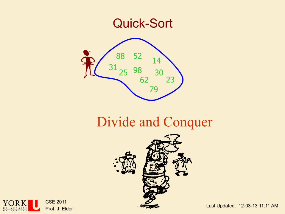
Quick-Sort
88 14 98 25
62
52
79
30 23
31
Divide and Conquer
Last Updated: 12-03-13 11:11 AM CSE 2011 Prof. J. Elder - 49 -
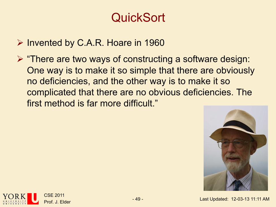
QuickSort
Ø Invented by C.A.R. Hoare in 1960
Ø “There are two ways of constructing a software design: One way is to make it so simple that there are obviously no deficiencies, and the other way is to make it so complicated that there are no obvious deficiencies. The first method is far more difficult.”
Last Updated: 12-03-13 11:11 AM CSE 2011 Prof. J. Elder - 50 -
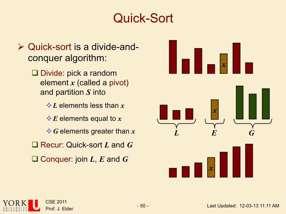
Quick-Sort
Ø Quick-sort is a divide-and-conquer algorithm: q Divide: pick a random
element x (called a pivot) and partition S into ² L elements less than x
² E elements equal to x
² G elements greater than x
q Recur: Quick-sort L and G
q Conquer: join L, E and G
x
x
L G E
x

Last Updated: 12-03-13 11:11 AM CSE 2011 Prof. J. Elder - 51 -
The Quick-Sort Algorithm
Algorithm QuickSort(S)
if S.size() > 1
(L, E, G) = Partition(S)
QuickSort(L) //Small elements are sorted
QuickSort(G) //Large elements are sorted
S = (L, E, G) //Thus input is sorted
Last Updated: 12-03-13 11:11 AM CSE 2011 Prof. J. Elder - 52 -
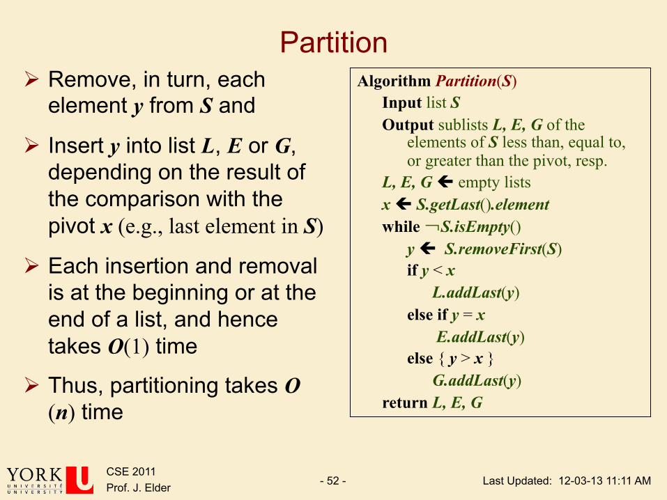
Partition Ø Remove, in turn, each
element y from S and
Ø Insert y into list L, E or G, depending on the result of the comparison with the pivot x (e.g., last element in S)
Ø Each insertion and removal is at the beginning or at the end of a list, and hence takes O(1) time
Ø Thus, partitioning takes O(n) time
Algorithm Partition(S) Input list S Output sublists L, E, G of the elements of S less than, equal to, or greater than the pivot, resp. L, E, G ç empty lists x ç S.getLast().element while S.isEmpty()
y ç S.removeFirst(S) if y < x L.addLast(y) else if y = x E.addLast(y) else { y > x } G.addLast(y)
return L, E, G
¬

Last Updated: 12-03-13 11:11 AM CSE 2011 Prof. J. Elder - 53 -
Partition Ø Since elements are
removed at the beginning and added at the end, this partition algorithm is stable.
Algorithm Partition(S) Input sequence S Output subsequences L, E, G of the elements of S less than, equal to, or greater than the pivot, resp. L, E, G ç empty sequences x ç S.getLast().element while S.isEmpty()
y ç S.removeFirst(S) if y < x L.addLast(y) else if y = x E.addLast(y) else { y > x } G.addLast(y)
return L, E, G
¬

Last Updated: 12-03-13 11:11 AM CSE 2011 Prof. J. Elder - 54 -
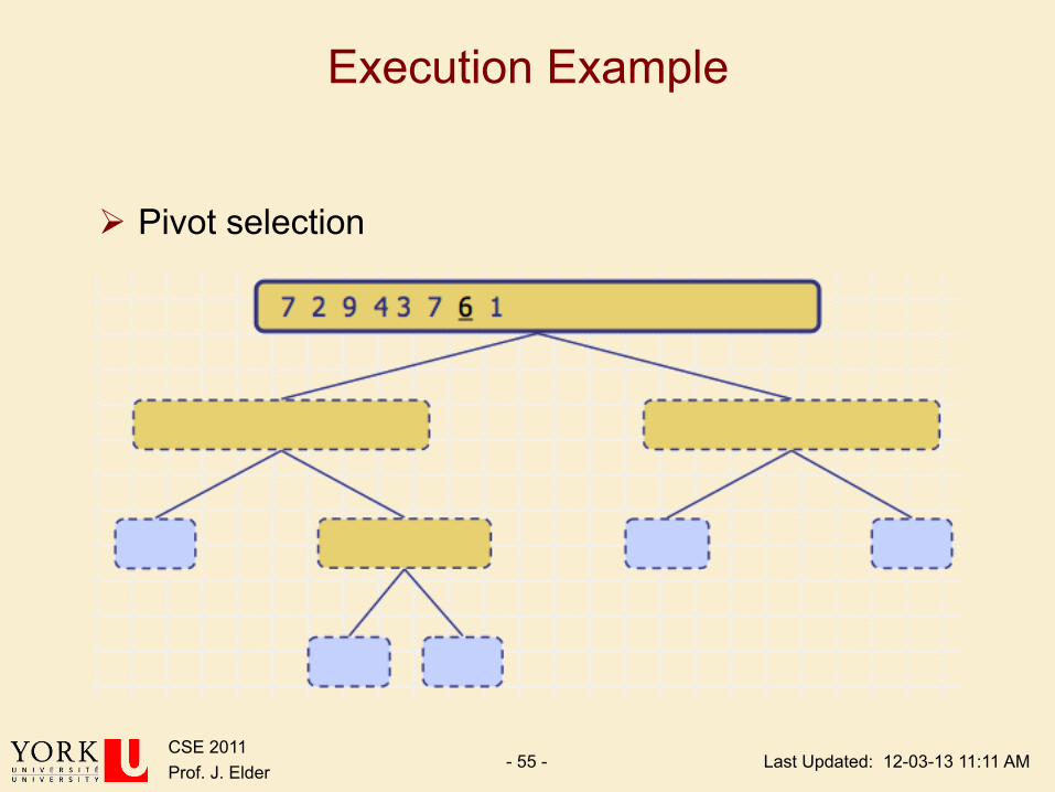
Quick-Sort Tree Ø An execution of quick-sort is depicted by a binary tree
q Each node represents a recursive call of quick-sort and stores ² Unsorted sequence before the execution and its pivot
² Sorted sequence at the end of the execution
q The root is the initial call
q The leaves are calls on subsequences of size 0 or 1
Last Updated: 12-03-13 11:11 AM CSE 2011 Prof. J. Elder - 55 -
Execution Example
Ø Pivot selection
Last Updated: 12-03-13 11:11 AM CSE 2011 Prof. J. Elder - 56 -
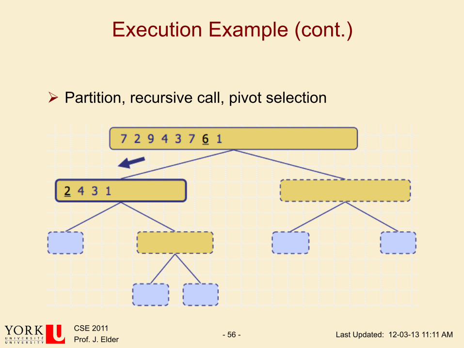
Execution Example (cont.)
Ø Partition, recursive call, pivot selection
Last Updated: 12-03-13 11:11 AM CSE 2011 Prof. J. Elder - 57 -
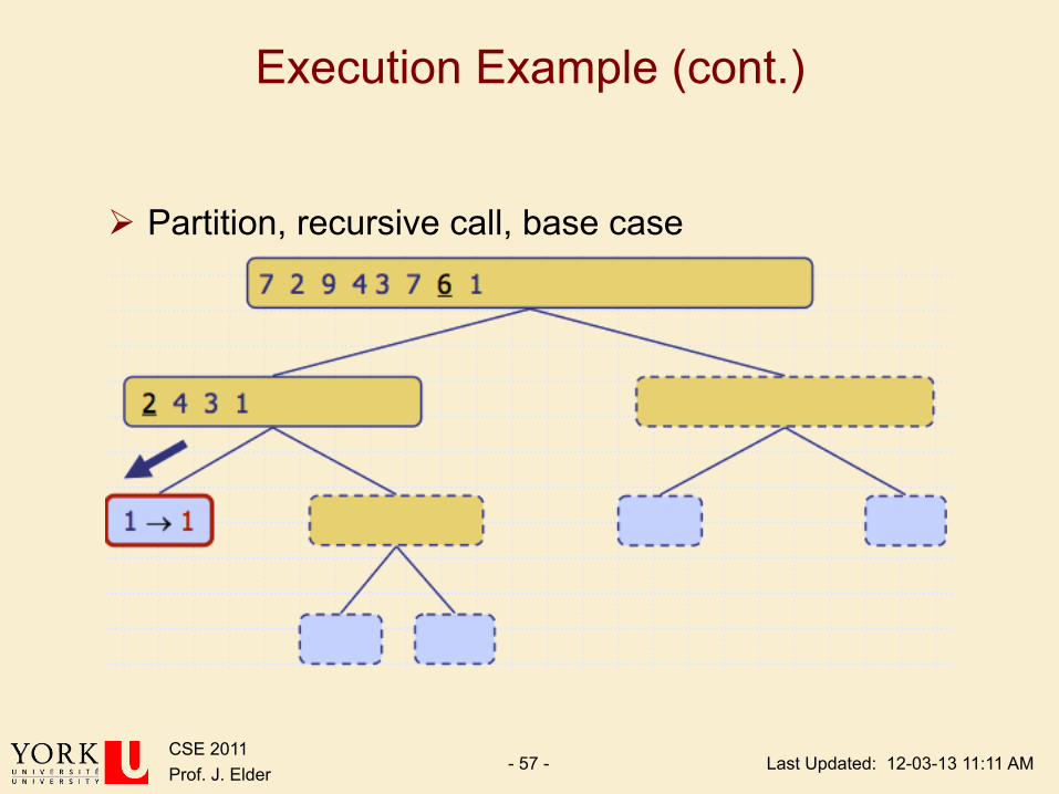
Execution Example (cont.)
Ø Partition, recursive call, base case
Last Updated: 12-03-13 11:11 AM CSE 2011 Prof. J. Elder - 58 -
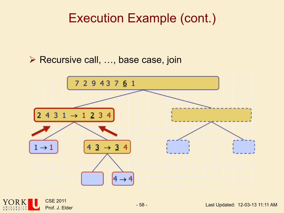
Execution Example (cont.)
Ø Recursive call, …, base case, join
Last Updated: 12-03-13 11:11 AM CSE 2011 Prof. J. Elder - 59 -
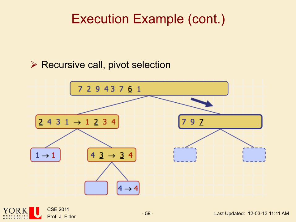
Execution Example (cont.)
Ø Recursive call, pivot selection

Last Updated: 12-03-13 11:11 AM CSE 2011 Prof. J. Elder - 60 -
Execution Example (cont.)
Ø Partition, …, recursive call, base case
Last Updated: 12-03-13 11:11 AM CSE 2011 Prof. J. Elder - 61 -
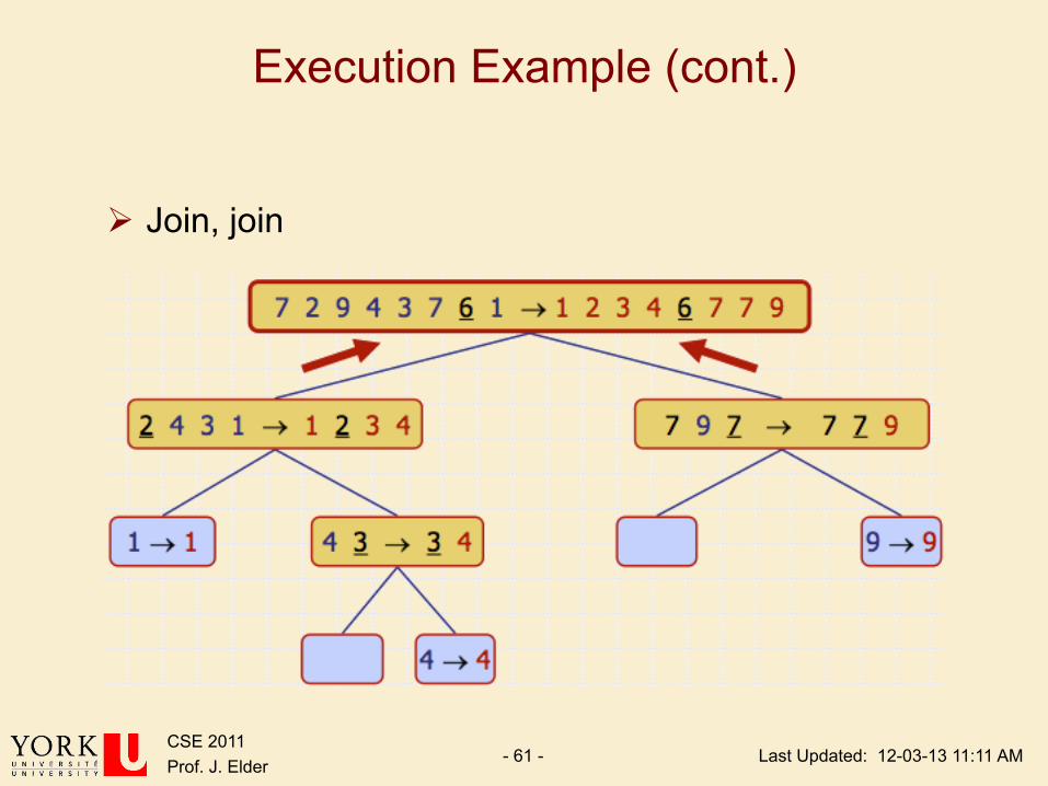
Execution Example (cont.)
Ø Join, join
Last Updated: 12-03-13 11:11 AM CSE 2011 Prof. J. Elder - 62 -
Quick-Sort Properties
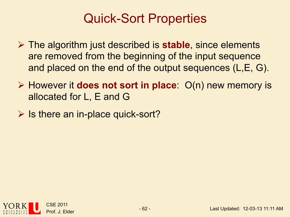
Ø The algorithm just described is stable, since elements are removed from the beginning of the input sequence and placed on the end of the output sequences (L,E, G).
Ø However it does not sort in place: O(n) new memory is allocated for L, E and G
Ø Is there an in-place quick-sort?

Last Updated: 12-03-13 11:11 AM CSE 2011 Prof. J. Elder - 63 -
In-Place Quick-Sort Ø Note: Use the lecture slides here instead of the textbook
implementation (Section 11.2.2)
88 14 98 25
62
52
79
30 23
31
Partition set into two using randomly chosen pivot
14
25 30
23 31
88 98 62
79 ≤ 52 <
Last Updated: 12-03-13 11:11 AM CSE 2011 Prof. J. Elder - 64 -
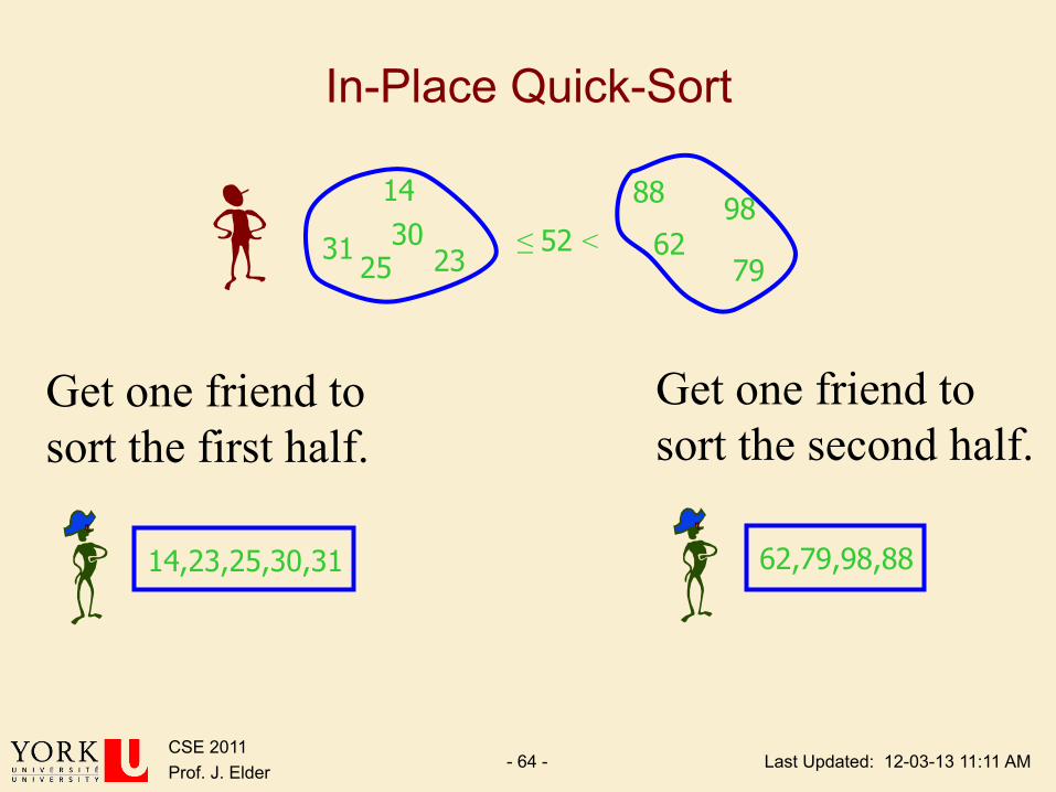
In-Place Quick-Sort
14
25 30
23 31
88 98 62
79 ≤ 52 <
14,23,25,30,31
Get one friend to sort the first half.
62,79,98,88
Get one friend to sort the second half.
Last Updated: 12-03-13 11:11 AM CSE 2011 Prof. J. Elder - 65 -
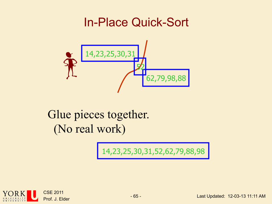
In-Place Quick-Sort
14,23,25,30,31
62,79,98,88 52
Glue pieces together. (No real work)
14,23,25,30,31,52,62,79,88,98
Last Updated: 12-03-13 11:11 AM CSE 2011 Prof. J. Elder - 66 -
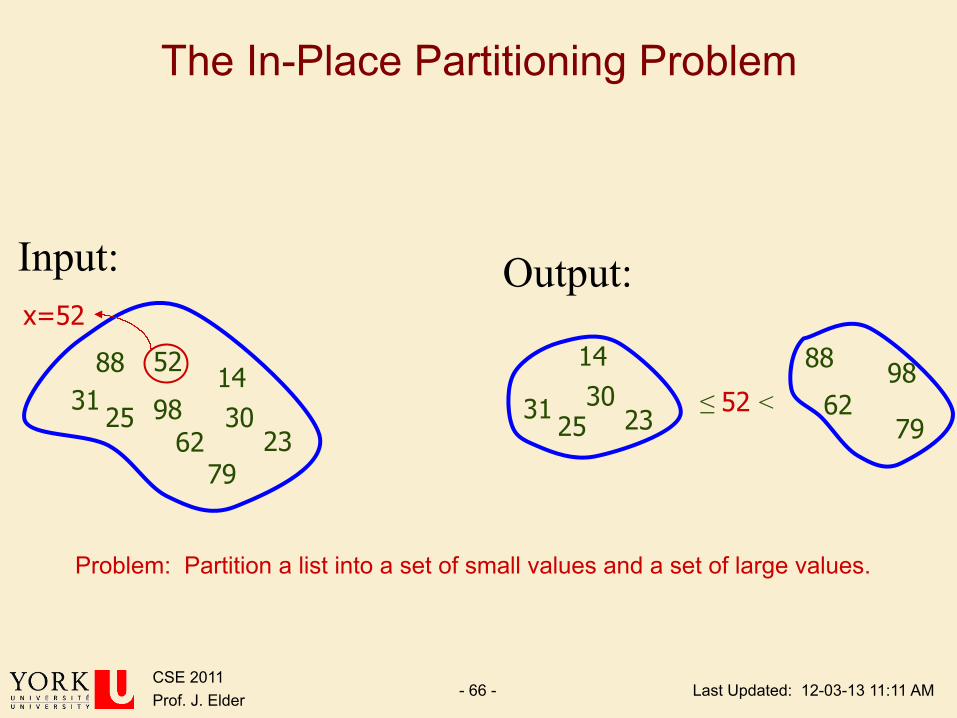
The In-Place Partitioning Problem
88 14 98 25
62
52
79
30 23
31
Input:
14
25 30
23 31
88 98 62
79 ≤ 52 <
Output: x=52
Problem: Partition a list into a set of small values and a set of large values.

Last Updated: 12-03-13 11:11 AM CSE 2011 Prof. J. Elder - 67 -
Precise Specification
[ ... ] is an arbitrary list of values. [ ] is the pivoPrecondit .i ton: A p r x A r=
p r
− ≤ = < + is rearranged such that [ ... 1] [ ] [ 1... ]for some Postcondition
q.: A A p q A q x A q r
p r q

Last Updated: 12-03-13 11:11 AM CSE 2011 Prof. J. Elder - 68 -
Ø 3 subsets are maintained q One containing values less
than or equal to the pivot
q One containing values greater than the pivot
q One containing values yet to be processed
Loop Invariant
Last Updated: 12-03-13 11:11 AM CSE 2011 Prof. J. Elder - 69 -
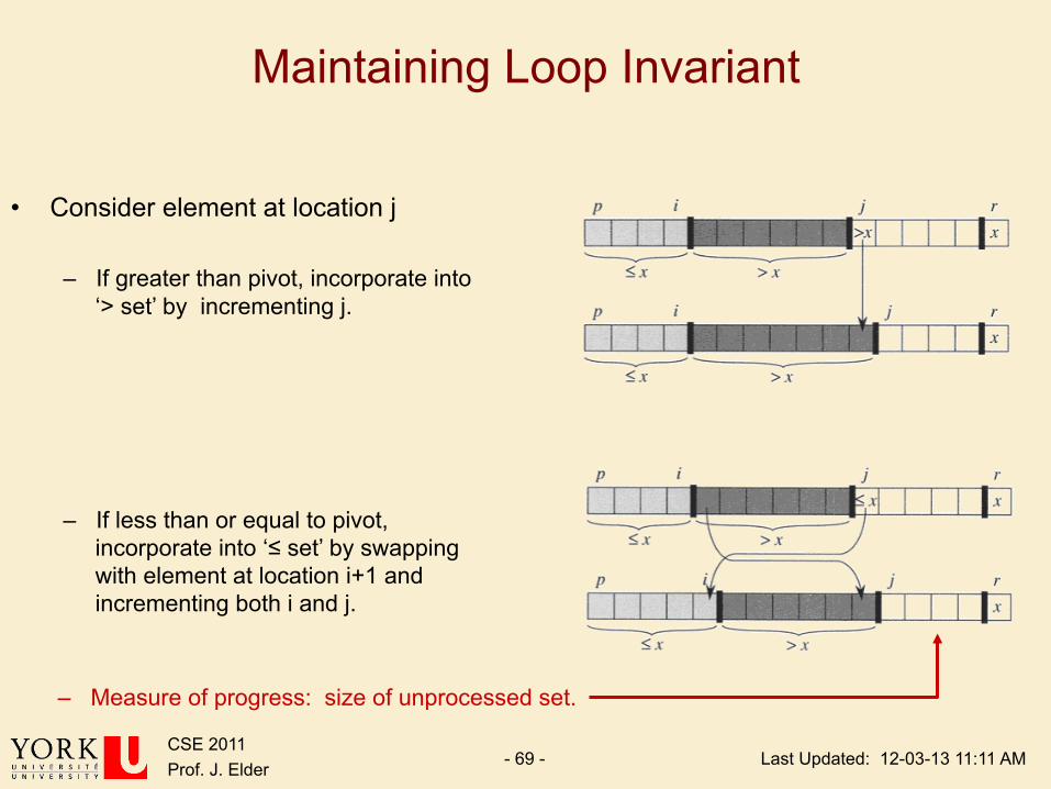
Maintaining Loop Invariant
• Consider element at location j
– If greater than pivot, incorporate into ‘> set’ by incrementing j.
– If less than or equal to pivot, incorporate into ‘≤ set’ by swapping with element at location i+1 and incrementing both i and j.
– Measure of progress: size of unprocessed set.
Last Updated: 12-03-13 11:11 AM CSE 2011 Prof. J. Elder - 70 -
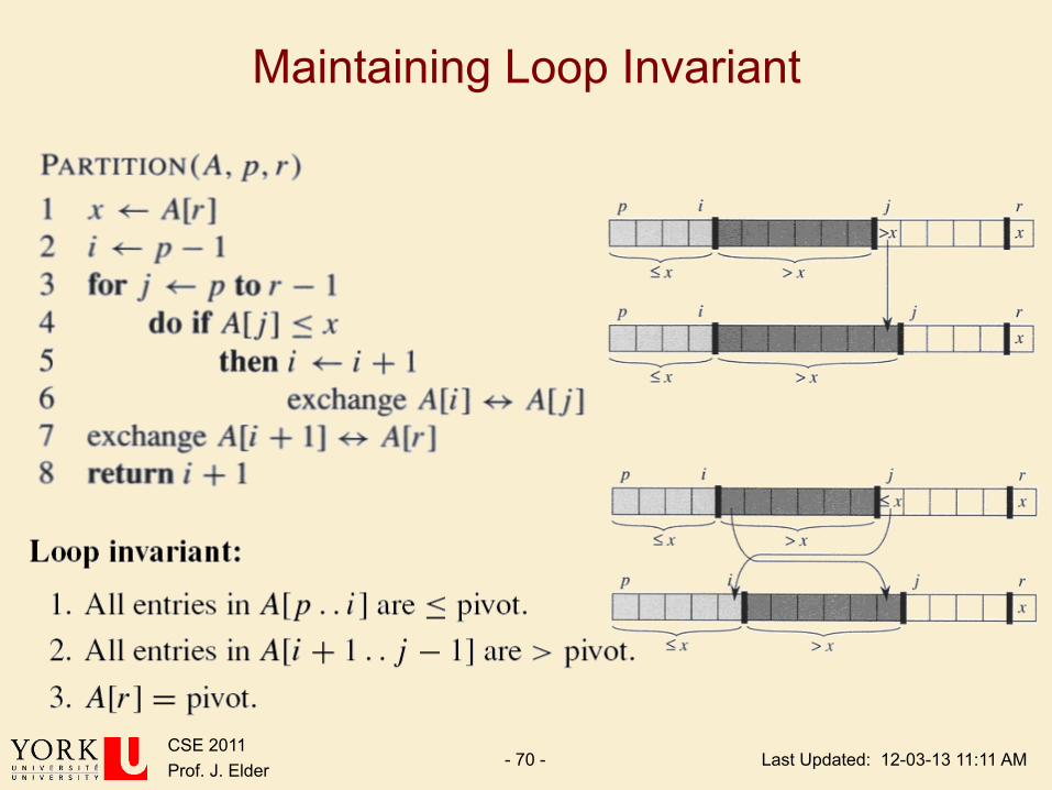
Maintaining Loop Invariant
Last Updated: 12-03-13 11:11 AM CSE 2011 Prof. J. Elder - 71 -
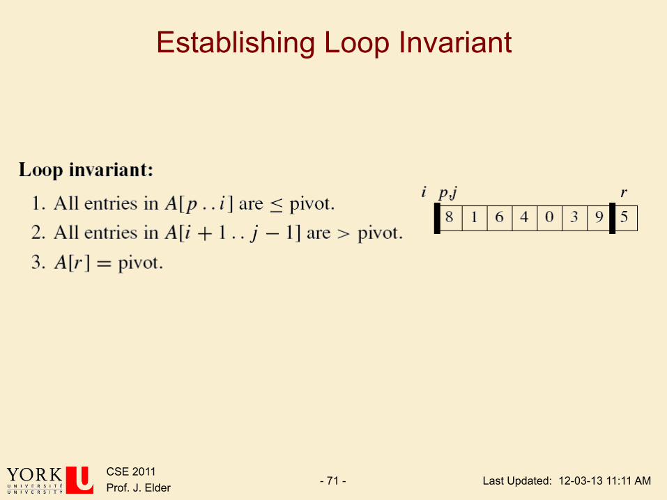
Establishing Loop Invariant
Last Updated: 12-03-13 11:11 AM CSE 2011 Prof. J. Elder - 72 -
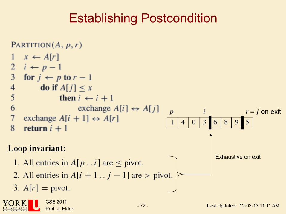
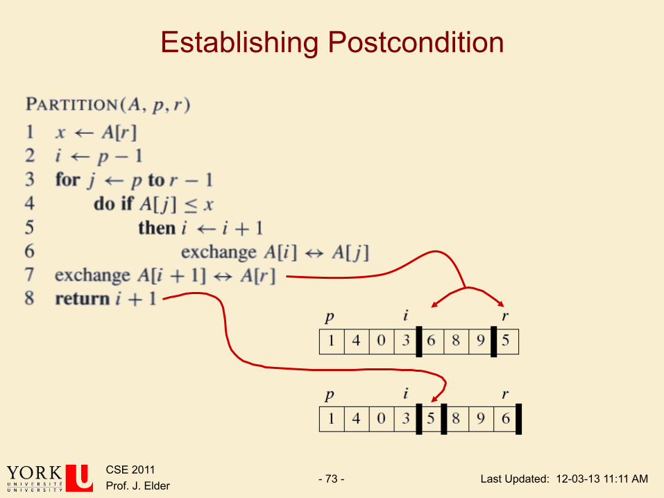
Establishing Postcondition
on exitj=
Exhaustive on exit
Last Updated: 12-03-13 11:11 AM CSE 2011 Prof. J. Elder - 73 -
Establishing Postcondition

Last Updated: 12-03-13 11:11 AM CSE 2011 Prof. J. Elder - 74 -
An Example
Last Updated: 12-03-13 11:11 AM CSE 2011 Prof. J. Elder - 75 -
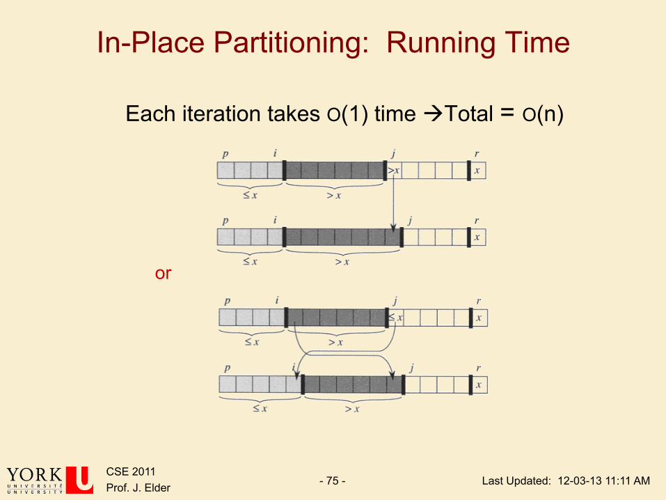
In-Place Partitioning: Running Time
Each iteration takes O(1) time àTotal = O(n)
or
Last Updated: 12-03-13 11:11 AM CSE 2011 Prof. J. Elder - 76 -
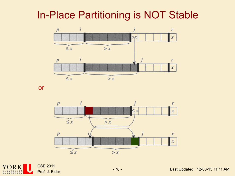
In-Place Partitioning is NOT Stable
or

Last Updated: 12-03-13 11:11 AM CSE 2011 Prof. J. Elder - 77 -
The In-Place Quick-Sort Algorithm
Algorithm QuickSort(A, p, r)
if p < r
q = Partition(A, p, r)
QuickSort(A, p, q - 1) //Small elements are sorted
QuickSort(A, q + 1, r) //Large elements are sorted
//Thus input is sorted
Last Updated: 12-03-13 11:11 AM CSE 2011 Prof. J. Elder - 78 -
Running Time of Quick-Sort
Last Updated: 12-03-13 11:11 AM CSE 2011 Prof. J. Elder - 79 -
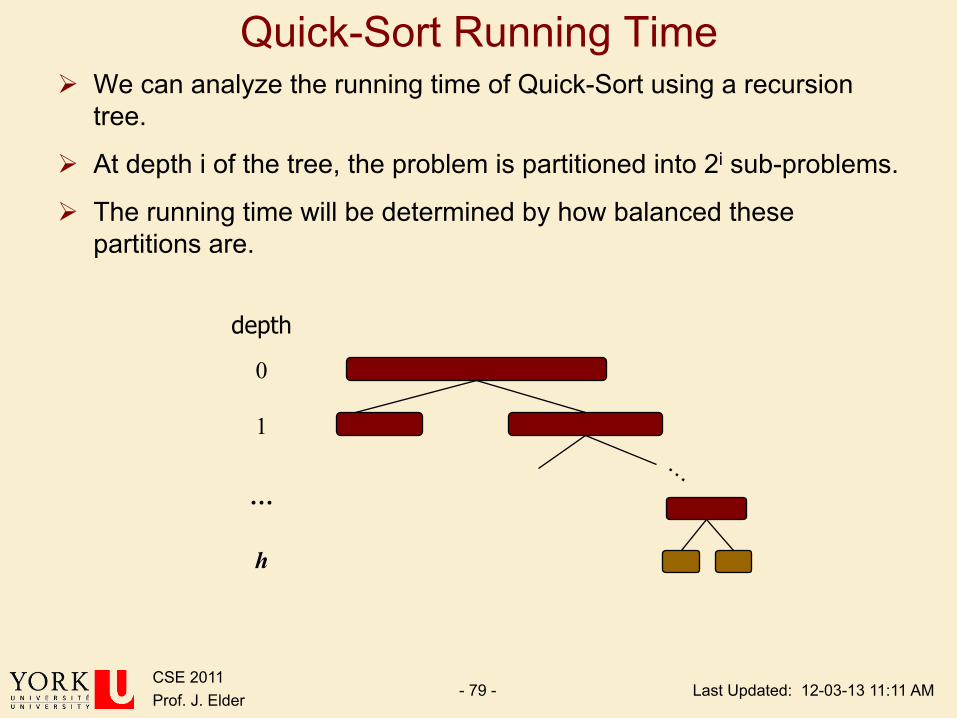
Quick-Sort Running Time Ø We can analyze the running time of Quick-Sort using a recursion
tree.
Ø At depth i of the tree, the problem is partitioned into 2i sub-problems.
Ø The running time will be determined by how balanced these partitions are.
depth
0
1
…
h
Last Updated: 12-03-13 11:11 AM CSE 2011 Prof. J. Elder - 80 -
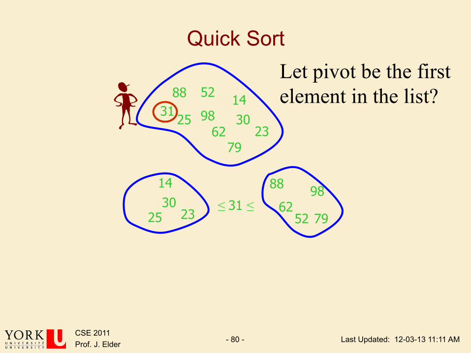
Quick Sort
88 14 98 25
62
52
79
30 23
31
Let pivot be the first element in the list?
14
25 30
23
88 98 62
79 ≤ 31 ≤
52
Last Updated: 12-03-13 11:11 AM CSE 2011 Prof. J. Elder - 81 -
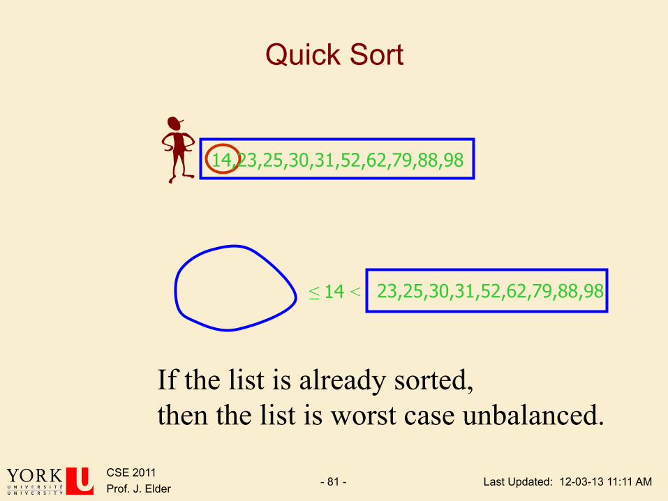
Quick Sort
≤ 14 <
14,23,25,30,31,52,62,79,88,98
23,25,30,31,52,62,79,88,98
If the list is already sorted, then the list is worst case unbalanced.

Last Updated: 12-03-13 11:11 AM CSE 2011 Prof. J. Elder - 82 -
QuickSort: Choosing the Pivot
Ø Common choices are: q random element
q middle element
q median of first, middle and last element
Last Updated: 12-03-13 11:11 AM CSE 2011 Prof. J. Elder - 83 -
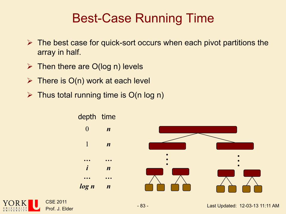
Best-Case Running Time
Ø The best case for quick-sort occurs when each pivot partitions the array in half.
Ø Then there are O(log n) levels
Ø There is O(n) work at each level
Ø Thus total running time is O(n log n)
depth time
0 n
1 n
… … i n
… … log n n
! !
Last Updated: 12-03-13 11:11 AM CSE 2011 Prof. J. Elder - 84 -
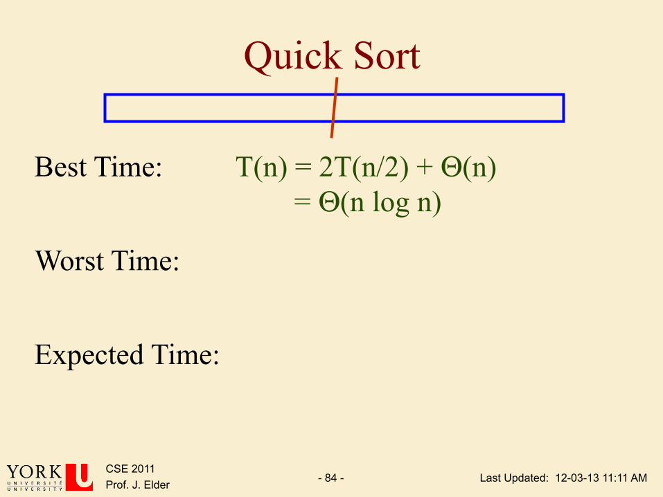
Quick Sort
Best Time:
Worst Time:
Expected Time:
T(n) = 2T(n/2) + Θ(n) = Θ(n log n)
Last Updated: 12-03-13 11:11 AM CSE 2011 Prof. J. Elder - 85 -
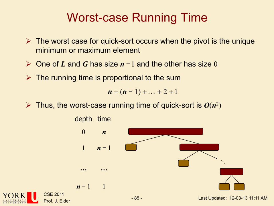
Worst-case Running Time
Ø The worst case for quick-sort occurs when the pivot is the unique minimum or maximum element
Ø One of L and G has size n - 1 and the other has size 0
Ø The running time is proportional to the sum
n + (n - 1) + … + 2 + 1
Ø Thus, the worst-case running time of quick-sort is O(n2)
depth time
0 n
1 n - 1
… …
n - 1 1
Last Updated: 12-03-13 11:11 AM CSE 2011 Prof. J. Elder - 86 -
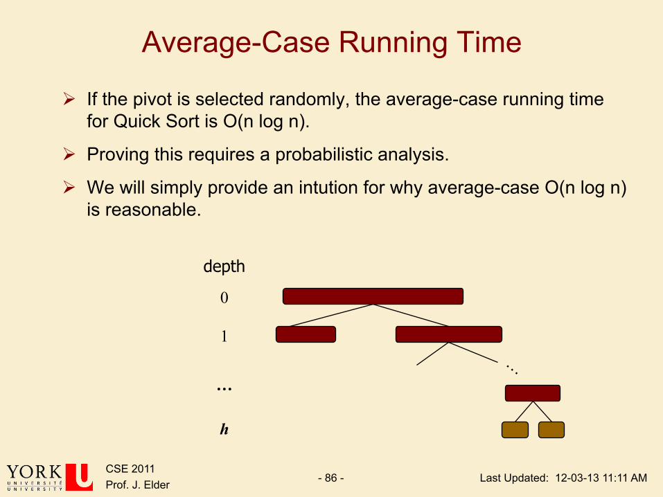
Average-Case Running Time
Ø If the pivot is selected randomly, the average-case running time for Quick Sort is O(n log n).
Ø Proving this requires a probabilistic analysis.
Ø We will simply provide an intution for why average-case O(n log n) is reasonable.
depth
0
1
…
h
Last Updated: 12-03-13 11:11 AM CSE 2011 Prof. J. Elder - 87 -
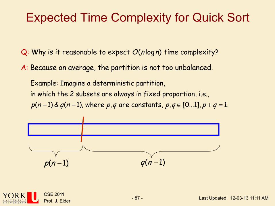
Expected Time Complexity for Quick Sort
Q: Why is it reasonable to expect O(n logn) time complexity?
Because on average, the partition is not too unbalanA: ced.
− − ∈ + =
Example: Imagine a deterministic partition, in which the 2 subsets are always in fixed proportion, i.e.,
( 1) & ( 1), where , are constants, , [0...1], 1.p n q n p q p q p q
( 1)p n − ( 1)q n −

Last Updated: 12-03-13 11:11 AM CSE 2011 Prof. J. Elder - 88 -
Expected Time Complexity for Quick Sort
( 1)p n − ( 1)q n −
Then T (n) =T (p(n ! 1)) +T (q(n ! 1)) +O(n)
wlog, suppose that q > p.Let k be the depth of the recursion tree Then qkn = 1 ! k = logn / log(1 / q)Thus k "O(logn) :
O(n) work done per level !T (n) = O(nlogn).

Last Updated: 12-03-13 11:11 AM CSE 2011 Prof. J. Elder - 89 -
Properties of QuickSort
Ø In-place?
Ø Stable?
Ø Fast? q Depends.
q Worst Case:
q Expected Case:
ü ü
2( )nΘ( log ), with small constantsn nΘ
But not both!

Last Updated: 12-03-13 11:11 AM CSE 2011 Prof. J. Elder - 90 -
Summary of Comparison Sorts
Algorithm Best Case
Worst Case
Average Case
In Place
Stable Comments
Selection n2
n2
Yes Yes
Bubble n
n2
Yes Yes Must count swaps for linear best case running time.
Insertion n n2
Yes Yes Good if often almost sorted
Merge n log n n log n No Yes Good for very large datasets that require swapping to disk
Heap n log n n log n Yes No Best if guaranteed n log n required
Quick n log n n2 n log n Yes Yes Usually fastest in practice
But not both!
Last Updated: 12-03-13 11:11 AM CSE 2011 Prof. J. Elder - 91 -
Comparison Sort: Lower Bound
MergeSort and HeapSort are both !(n logn) (worst case).
Can we do better?
Last Updated: 12-03-13 11:11 AM CSE 2011 Prof. J. Elder - 92 -
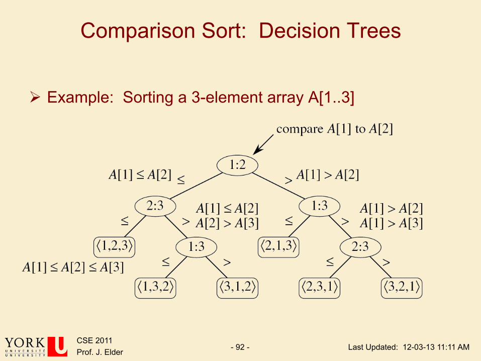
Comparison Sort: Decision Trees
Ø Example: Sorting a 3-element array A[1..3]
Last Updated: 12-03-13 11:11 AM CSE 2011 Prof. J. Elder - 93 -
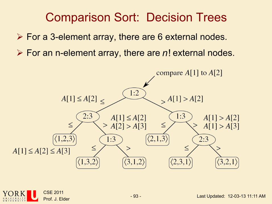
Comparison Sort: Decision Trees Ø For a 3-element array, there are 6 external nodes.
Ø For an n-element array, there are external nodes. n!

Last Updated: 12-03-13 11:11 AM CSE 2011 Prof. J. Elder - 94 -
Comparison Sort
Ø To store n! external nodes, a decision tree must have a height of at least
Ø Worst-case time is equal to the height of the binary decision tree.
Thus T(n)!" logn!( )where logn! = log i
i=1
n
# $ log n / 2%& '(i=1
n / 2%& '(
# !"(n logn)
Thus T(n)!"(n logn)
Thus MergeSort & HeapSort are asymptotically optimal.
logn!!" #$
Last Updated: 12-03-13 11:11 AM CSE 2011 Prof. J. Elder - 95 -
Linear Sorts?
Comparison sorts are very general, but are ( log )n nΩ
Faster sorting may be possible if we can constrain the nature of the input.

Last Updated: 12-03-13 11:11 AM CSE 2011 Prof. J. Elder - 96 -
Example 1. Counting Sort
Ø Invented by Harold Seward in 1954.
Ø Counting Sort applies when the elements to be sorted come from a finite (and preferably small) set.
Ø For example, the elements to be sorted are integers in the range [0…k-1], for some fixed integer k.
Ø We can then create an array V[0…k-1] and use it to count the number of elements with each value [0…k-1].
Ø Then each input element can be placed in exactly the right place in the output array in constant time.
Last Updated: 12-03-13 11:11 AM CSE 2011 Prof. J. Elder - 97 -
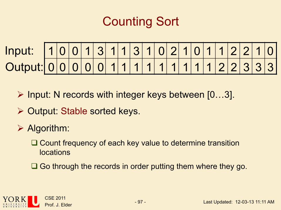
Counting Sort
Ø Input: N records with integer keys between [0…3].
Ø Output: Stable sorted keys.
Ø Algorithm: q Count frequency of each key value to determine transition
locations
q Go through the records in order putting them where they go.
Input: Output: 0 0 0 0 0 1 1 1 1 1 1 1 1 1 2 2 3 3 3
1 0 0 1 3 1 1 3 1 0 2 1 0 1 1 2 2 1 0
Last Updated: 12-03-13 11:11 AM CSE 2011 Prof. J. Elder - 98 -
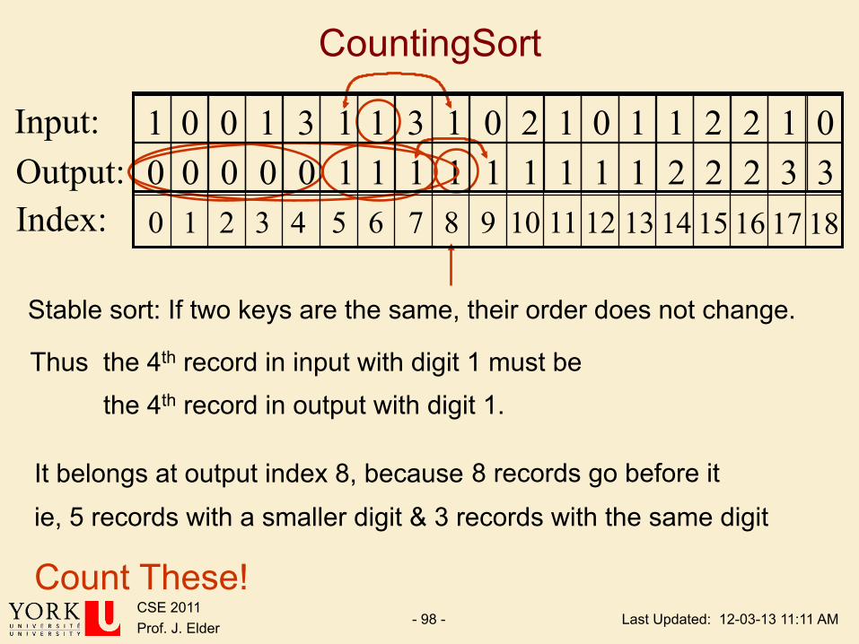
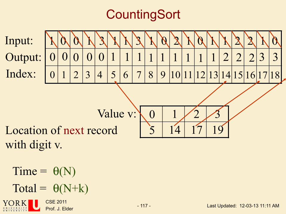
CountingSort
Stable sort: If two keys are the same, their order does not change.
Input: Output:
1 0 0 1 3 1 1 3 1 0 2 1 0 1 1 2 2 1 0
Thus the 4th record in input with digit 1 must be the 4th record in output with digit 1.
It belongs at output index 8, because 8 records go before it
ie, 5 records with a smaller digit & 3 records with the same digit
0 0 0 0 0 1 1 1 1 1 1 1 1 1 2 2 2 3 3
Count These!
Index: 11 10 9 8 7 6 5 4 3 2 1 0 12 13 14 15 16 17 18
Last Updated: 12-03-13 11:11 AM CSE 2011 Prof. J. Elder - 99 -
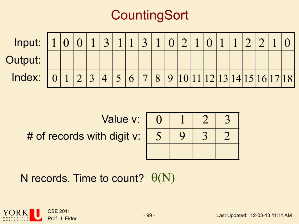
CountingSort
Input: Output:
Index: 11 10 9 8 7 6 5 4 3 2 1 0 12 13 14 15 16 17 18
Value v: # of records with digit v:
1 0 0 1 3 1 1 3 1 0 2 1 0 1 1 2 2 1 0
3 2 1 0 2 3 9 5
N records. Time to count? θ(N)
Last Updated: 12-03-13 11:11 AM CSE 2011 Prof. J. Elder - 100 -
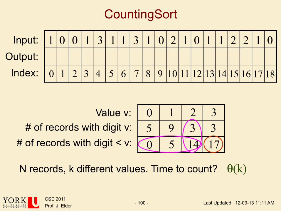
CountingSort
Input: Output:
Index: 11 10 9 8 7 6 5 4 3 2 1 0 12 13 14 15 16 17 18
Value v: # of records with digit v:
# of records with digit < v:
1 0 0 1 3 1 1 3 1 0 2 1 0 1 1 2 2 1 0
3 2 1 0 3 3 9 5 17 14 5 0
N records, k different values. Time to count? θ(k)
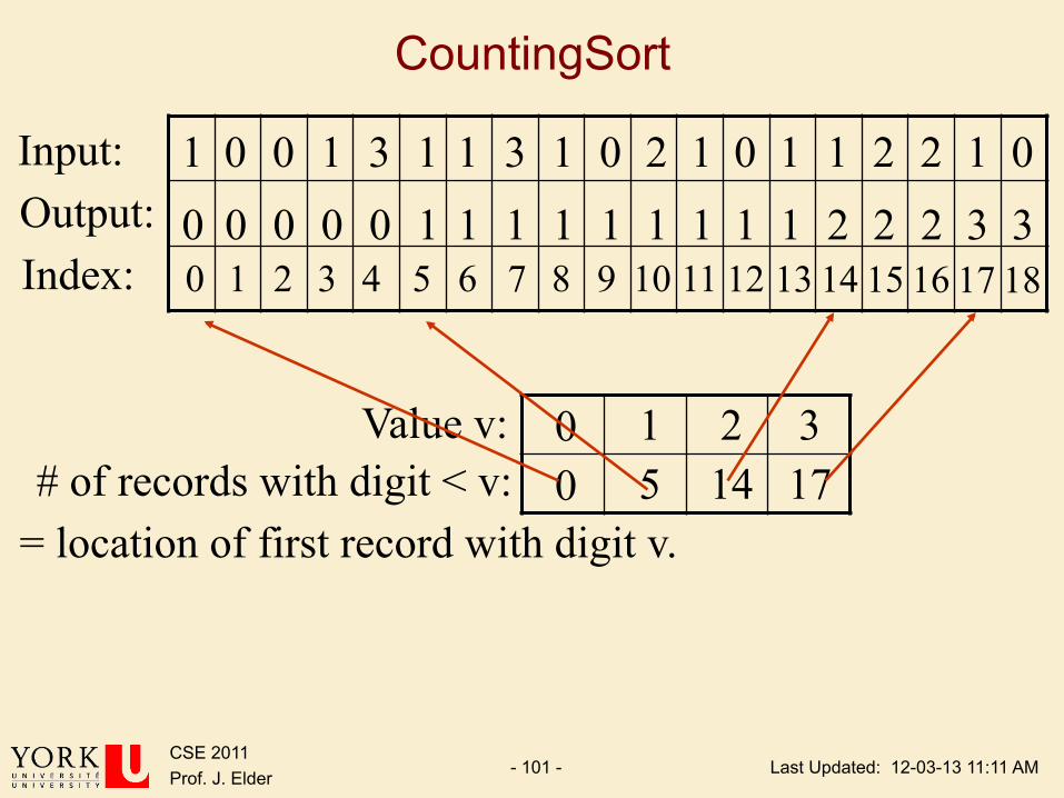
Last Updated: 12-03-13 11:11 AM CSE 2011 Prof. J. Elder - 101 -
CountingSort
Input: Output: Index: 11 10 9 8 7 6 5 4 3 2 1 0 12 13 14 15 16 17 18
Value v: # of records with digit < v:
1 0 0 1 3 1 1 3 1 0 2 1 0 1 1 2 2 1 0
3 2 1 0 17 14 5 0
= location of first record with digit v.
0 0 0 0 0 1 1 1 1 1 1 1 1 1 2 2 2 3 3
Last Updated: 12-03-13 11:11 AM CSE 2011 Prof. J. Elder - 102 -
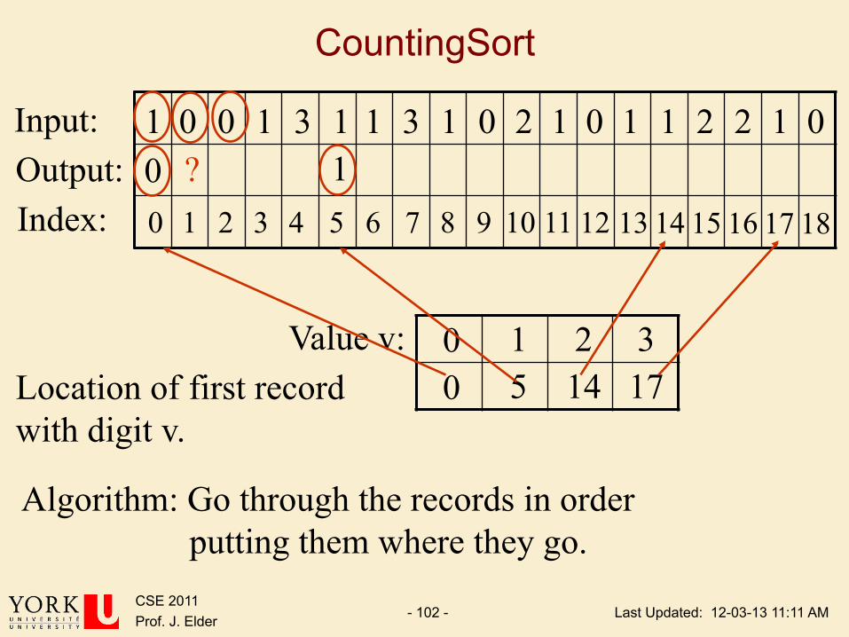
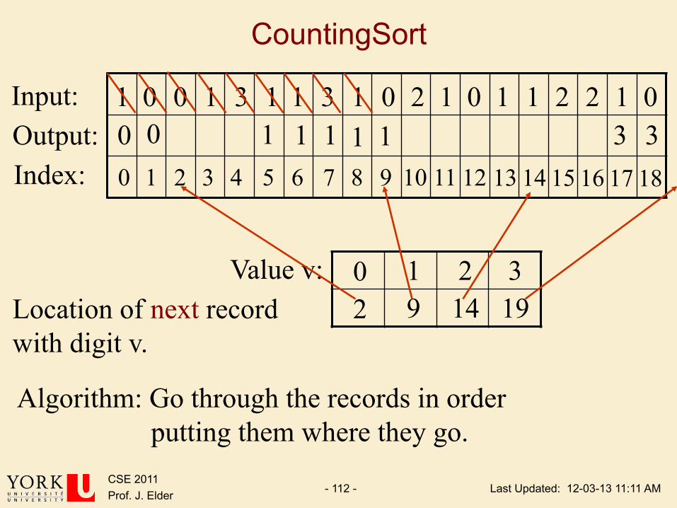
CountingSort
Input: Output: Index: 11 10 9 8 7 6 5 4 3 2 1 0 12 13 14 15 16 17 18
Value v:
1 0 0 1 3 1 1 3 1 0 2 1 0 1 1 2 2 1 0
3 2 1 0 17 14 5 0 Location of first record
with digit v.
Algorithm: Go through the records in order putting them where they go.
1 0 ?

Last Updated: 12-03-13 11:11 AM CSE 2011 Prof. J. Elder - 103 -
Loop Invariant
Ø The first i-1 keys have been placed in the correct locations in the output array
Ø The auxiliary data structure v indicates the location at which to place the ith key for each possible key value from [0..k-1].
Last Updated: 12-03-13 11:11 AM CSE 2011 Prof. J. Elder - 104 -
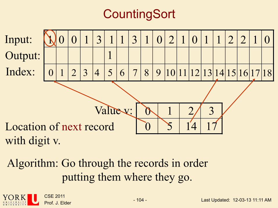
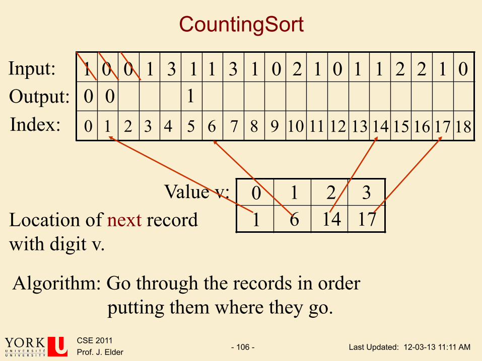
CountingSort
Input: Output: Index: 11 10 9 8 7 6 5 4 3 2 1 0 12 13 14 15 16 17 18
Value v:
1 0 0 1 3 1 1 3 1 0 2 1 0 1 1 2 2 1 0
3 2 1 0 17 14 5 0 Location of next record
with digit v.
1
Algorithm: Go through the records in order putting them where they go.
Last Updated: 12-03-13 11:11 AM CSE 2011 Prof. J. Elder - 105 -
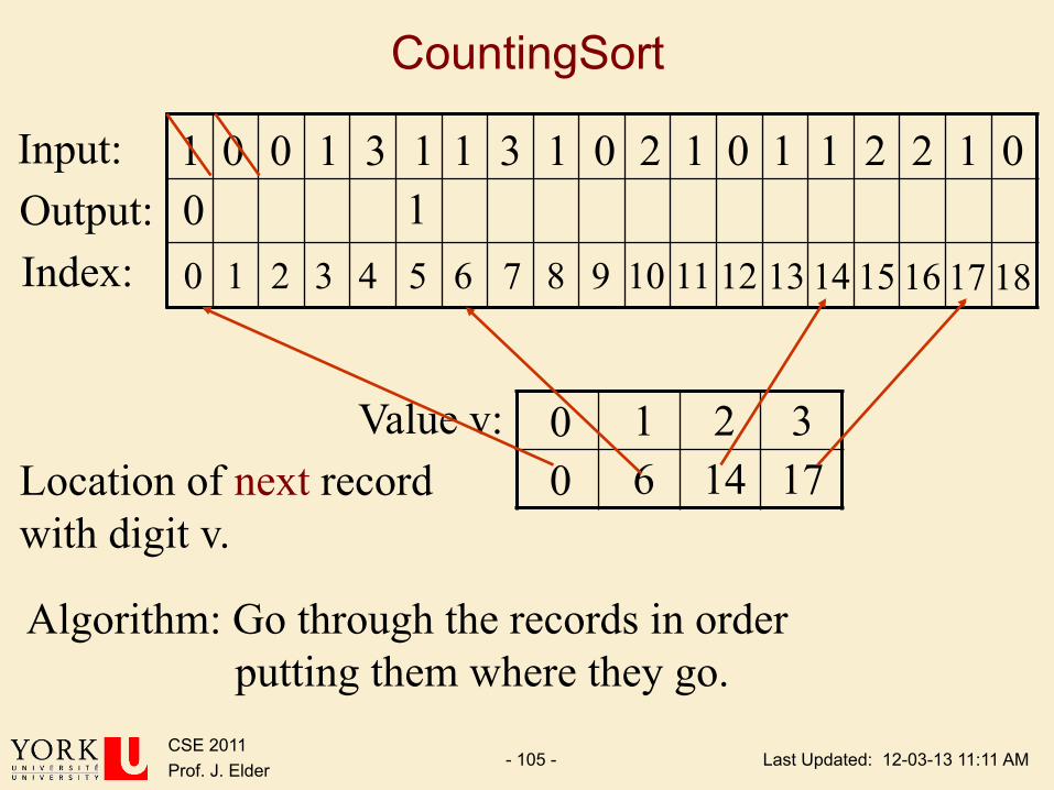
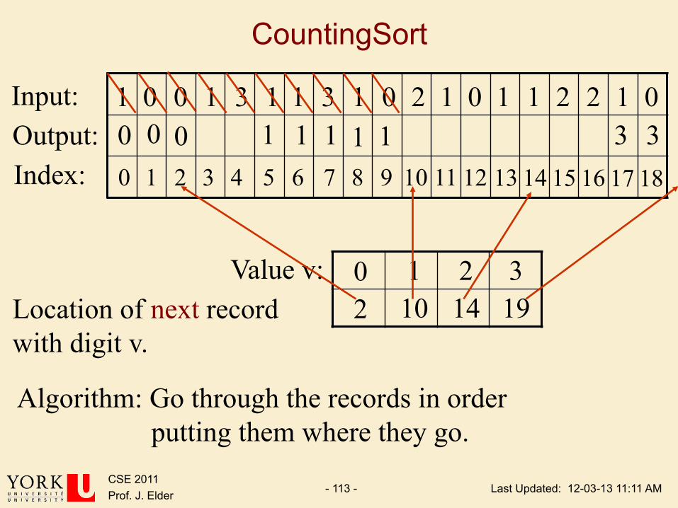
CountingSort
Input: Output: Index: 11 10 9 8 7 6 5 4 3 2 1 0 12 13 14 15 16 17 18
Value v:
1 0 0 1 3 1 1 3 1 0 2 1 0 1 1 2 2 1 0
3 2 1 0 17 14 6 0 Location of next record
with digit v.
0
Algorithm: Go through the records in order putting them where they go.
1
Last Updated: 12-03-13 11:11 AM CSE 2011 Prof. J. Elder - 106 -
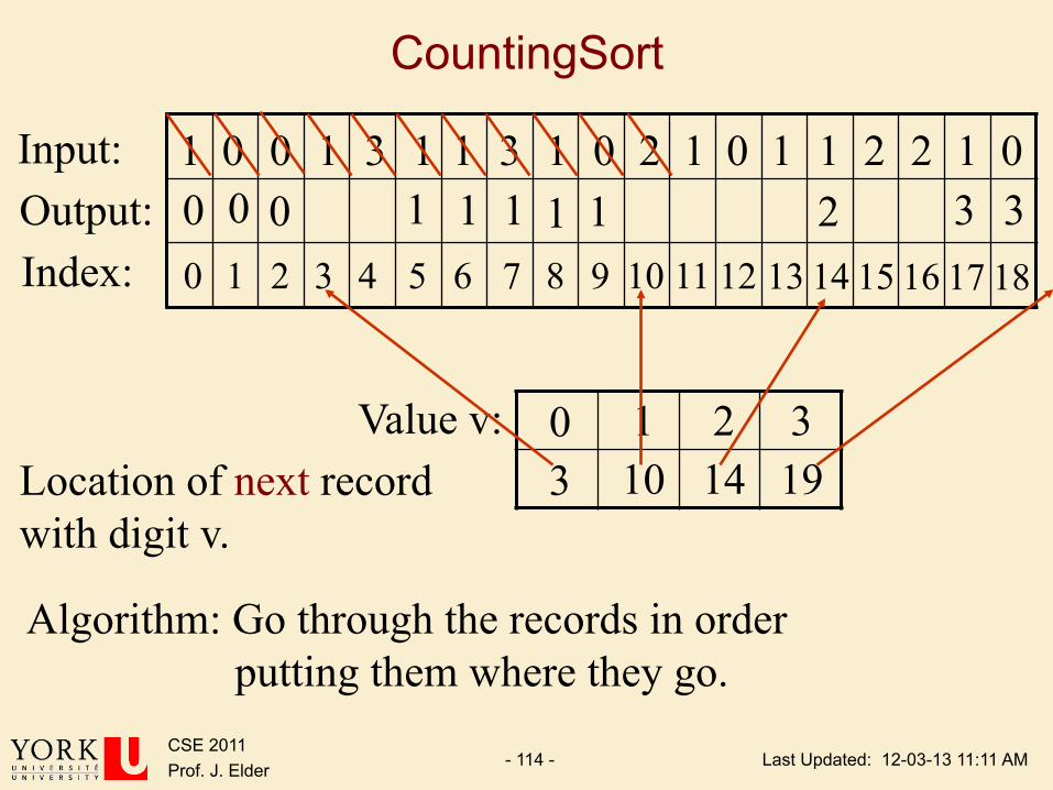
CountingSort
Input: Output: Index: 11 10 9 8 7 6 5 4 3 2 1 0 12 13 14 15 16 17 18
Value v:
1 0 0 1 3 1 1 3 1 0 2 1 0 1 1 2 2 1 0
3 2 1 0 17 14 6 1 Location of next record
with digit v.
0 0
Algorithm: Go through the records in order putting them where they go.
1
Last Updated: 12-03-13 11:11 AM CSE 2011 Prof. J. Elder - 107 -
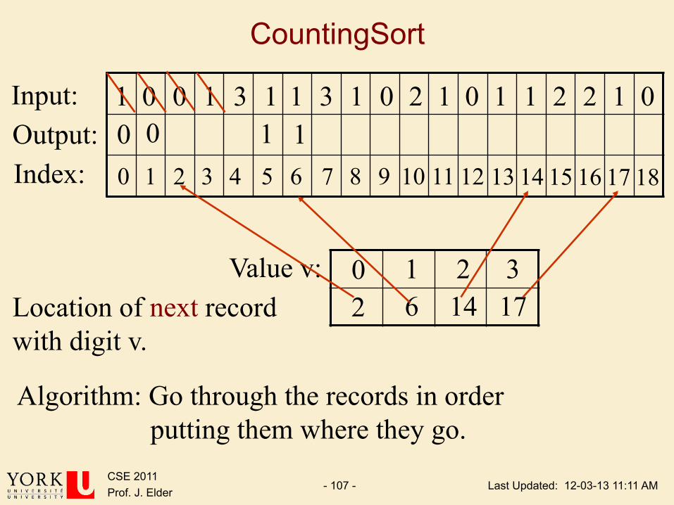
CountingSort
Input: Output: Index: 11 10 9 8 7 6 5 4 3 2 1 0 12 13 14 15 16 17 18
Value v:
1 0 0 1 3 1 1 3 1 0 2 1 0 1 1 2 2 1 0
3 2 1 0 17 14 6 2 Location of next record
with digit v.
0 1
Algorithm: Go through the records in order putting them where they go.
1 0

Last Updated: 12-03-13 11:11 AM CSE 2011 Prof. J. Elder - 108 -
CountingSort
Input: Output: Index: 11 10 9 8 7 6 5 4 3 2 1 0 12 13 14 15 16 17 18
Value v:
1 0 0 1 3 1 1 3 1 0 2 1 0 1 1 2 2 1 0
3 2 1 0 17 14 7 2 Location of next record
with digit v.
0 1
Algorithm: Go through the records in order putting them where they go.
1 0 3
Last Updated: 12-03-13 11:11 AM CSE 2011 Prof. J. Elder - 109 -
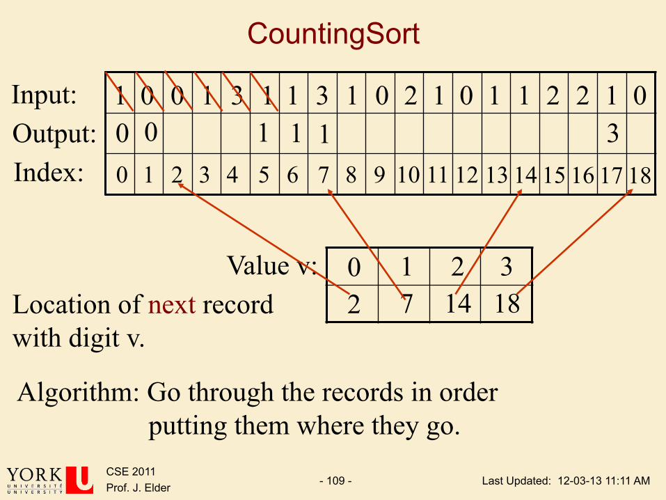
CountingSort
Input: Output: Index: 11 10 9 8 7 6 5 4 3 2 1 0 12 13 14 15 16 17 18
Value v:
1 0 0 1 3 1 1 3 1 0 2 1 0 1 1 2 2 1 0
3 2 1 0 18 14 7 2 Location of next record
with digit v.
0 1
Algorithm: Go through the records in order putting them where they go.
1 0 1 3
Last Updated: 12-03-13 11:11 AM CSE 2011 Prof. J. Elder - 110 -
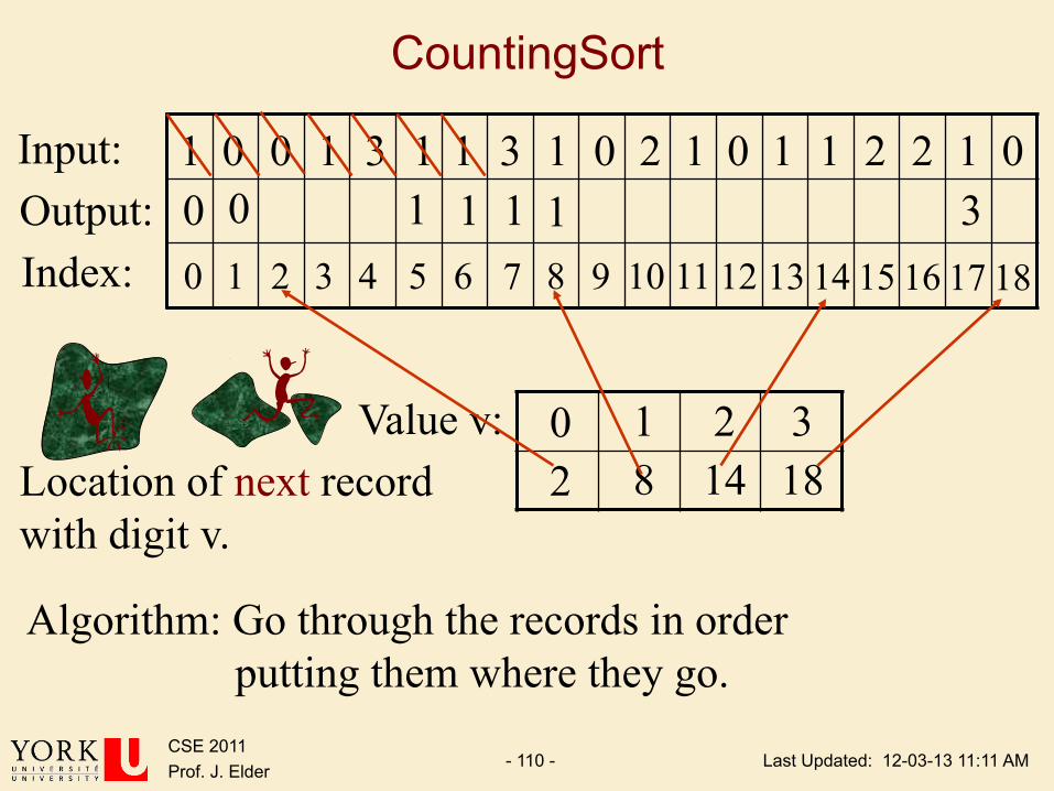
CountingSort
Input: Output: Index: 11 10 9 8 7 6 5 4 3 2 1 0 12 13 14 15 16 17 18
Value v:
1 0 0 1 3 1 1 3 1 0 2 1 0 1 1 2 2 1 0
3 2 1 0 18 14 8 2 Location of next record
with digit v.
0 1
Algorithm: Go through the records in order putting them where they go.
1 0 1 3 1

Last Updated: 12-03-13 11:11 AM CSE 2011 Prof. J. Elder - 111 -
CountingSort
Input: Output: Index: 11 10 9 8 7 6 5 4 3 2 1 0 12 13 14 15 16 17 18
Value v:
1 0 0 1 3 1 1 3 1 0 2 1 0 1 1 2 2 1 0
3 2 1 0 18 14 9 2 Location of next record
with digit v.
0 1
Algorithm: Go through the records in order putting them where they go.
1 0 3 3 1 1
Last Updated: 12-03-13 11:11 AM CSE 2011 Prof. J. Elder - 112 -
CountingSort
Input: Output: Index: 11 10 9 8 7 6 5 4 3 2 1 0 12 13 14 15 16 17 18
Value v:
1 0 0 1 3 1 1 3 1 0 2 1 0 1 1 2 2 1 0
3 2 1 0 19 14 9 2 Location of next record
with digit v.
0 1
Algorithm: Go through the records in order putting them where they go.
1 0 1 3 1 1 3
Last Updated: 12-03-13 11:11 AM CSE 2011 Prof. J. Elder - 113 -
CountingSort
Input: Output: Index: 11 10 9 8 7 6 5 4 3 2 1 0 12 13 14 15 16 17 18
Value v:
1 0 0 1 3 1 1 3 1 0 2 1 0 1 1 2 2 1 0
3 2 1 0 19 14 10 2 Location of next record
with digit v.
0 1
Algorithm: Go through the records in order putting them where they go.
1 0 0 1 1 1 3 3
Last Updated: 12-03-13 11:11 AM CSE 2011 Prof. J. Elder - 114 -
CountingSort
Input: Output: Index: 11 10 9 8 7 6 5 4 3 2 1 0 12 13 14 15 16 17 18
Value v:
1 0 0 1 3 1 1 3 1 0 2 1 0 1 1 2 2 1 0
3 2 1 0 19 14 10 3 Location of next record
with digit v.
0 1
Algorithm: Go through the records in order putting them where they go.
1 0 2 1 1 1 3 3 0

Last Updated: 12-03-13 11:11 AM CSE 2011 Prof. J. Elder - 115 -
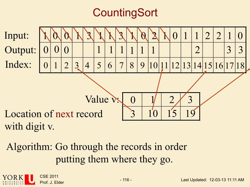
CountingSort
Input: Output: Index: 11 10 9 8 7 6 5 4 3 2 1 0 12 13 14 15 16 17 18
Value v:
1 0 0 1 3 1 1 3 1 0 2 1 0 1 1 2 2 1 0
3 2 1 0 19 15 10 3 Location of next record
with digit v.
0 1
Algorithm: Go through the records in order putting them where they go.
1 0 1 1 1 1 3 3 0 2
Last Updated: 12-03-13 11:11 AM CSE 2011 Prof. J. Elder - 116 -
CountingSort
Input: Output: Index: 11 10 9 8 7 6 5 4 3 2 1 0 12 13 14 15 16 17 18
Value v:
1 0 0 1 3 1 1 3 1 0 2 1 0 1 1 2 2 1 0
3 2 1 0 19 15 10 3 Location of next record
with digit v.
0 1
Algorithm: Go through the records in order putting them where they go.
1 0 1 1 1 1 3 3 0 2
Last Updated: 12-03-13 11:11 AM CSE 2011 Prof. J. Elder - 117 -
CountingSort
Input: Output: Index: 11 10 9 8 7 6 5 4 3 2 1 0 12 13 14 15 16 17 18
Value v:
1 0 0 1 3 1 1 3 1 0 2 1 0 1 1 2 2 1 0
3 2 1 0 19 17 14 5 Location of next record
with digit v.
0 1 1 0 1 1 1 1 3 3 0 2 0 0 1 1 1 2 2
θ(N) Time = θ(N+k) Total =
Last Updated: 12-03-13 11:11 AM CSE 2011 Prof. J. Elder - 118 -
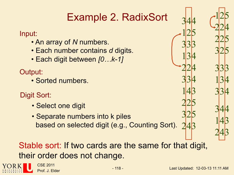
Input: • An array of N numbers. • Each number contains d digits. • Each digit between [0…k-1]
Output: • Sorted numbers.
Example 2. RadixSort 344 125 333 134 224 334 143 225 325 243
Digit Sort: • Select one digit • Separate numbers into k piles based on selected digit (e.g., Counting Sort).
125 224 225 325
333 134 334
344 143 243
Stable sort: If two cards are the same for that digit, their order does not change.
Last Updated: 12-03-13 11:11 AM CSE 2011 Prof. J. Elder - 119 -
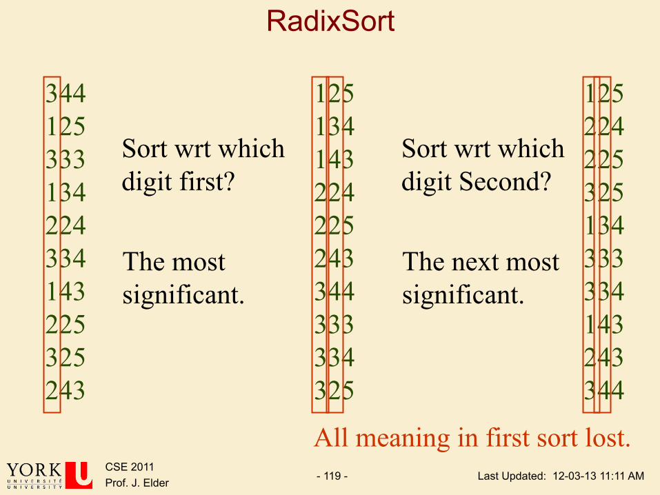
RadixSort
344 125 333 134 224 334 143 225 325 243
Sort wrt which digit first?
The most significant.
125 134 143 224 225 243 344 333 334 325
Sort wrt which digit Second?
The next most significant.
125 224 225 325 134 333 334 143 243 344
All meaning in first sort lost.
Last Updated: 12-03-13 11:11 AM CSE 2011 Prof. J. Elder - 120 -
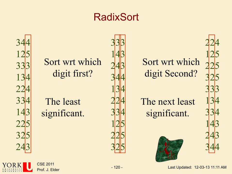
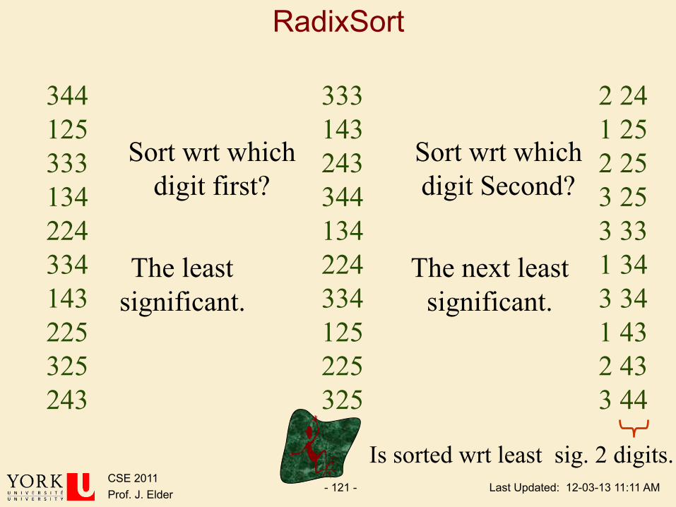
RadixSort
344 125 333 134 224 334 143 225 325 243
Sort wrt which digit first?
Sort wrt which digit Second?
The least significant.
333 143 243 344 134 224 334 125 225 325
The next least significant.
224 125 225 325 333 134 334 143 243 344
Last Updated: 12-03-13 11:11 AM CSE 2011 Prof. J. Elder - 121 -
RadixSort
344 125 333 134 224 334 143 225 325 243
Sort wrt which digit first?
Sort wrt which digit Second?
The least significant.
333 143 243 344 134 224 334 125 225 325
The next least significant.
2 24 1 25 2 25 3 25 3 33 1 34 3 34 1 43 2 43 3 44 Is sorted wrt least sig. 2 digits.
Last Updated: 12-03-13 11:11 AM CSE 2011 Prof. J. Elder - 122 -
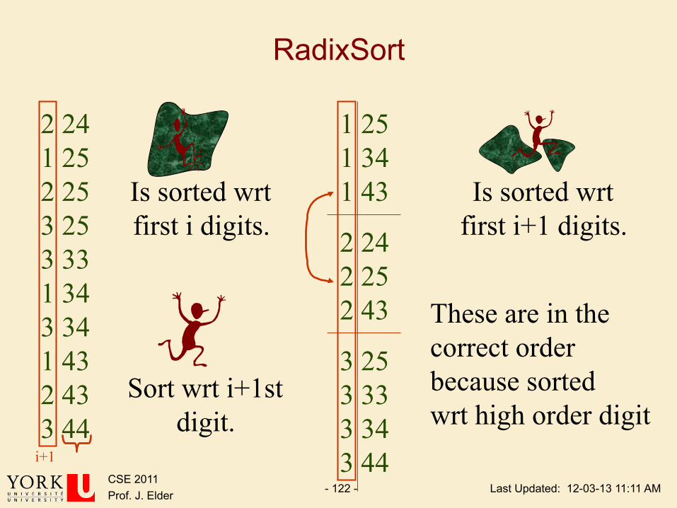
Sort wrt i+1st digit.
2 24 1 25 2 25 3 25 3 33 1 34 3 34 1 43 2 43 3 44
Is sorted wrt first i digits.
1 25 1 34 1 43
2 24 2 25 2 43
3 25 3 33 3 34 3 44
Is sorted wrt first i+1 digits.
i+1
These are in the correct order because sorted wrt high order digit
RadixSort

Last Updated: 12-03-13 11:11 AM CSE 2011 Prof. J. Elder - 123 -
Sort wrt i+1st digit.
2 24 1 25 2 25 3 25 3 33 1 34 3 34 1 43 2 43 3 44
Is sorted wrt first i digits.
1 25 1 34 1 43
2 24 2 25 2 43
3 25 3 33 3 34 3 44
i+1
These are in the correct order because was sorted & stable sort left sorted
Is sorted wrt first i+1 digits.
RadixSort
Last Updated: 12-03-13 11:11 AM CSE 2011 Prof. J. Elder - 124 -
Loop Invariant
Ø The keys have been correctly stable-sorted with respect to the i-1 least-significant digits.

Last Updated: 12-03-13 11:11 AM CSE 2011 Prof. J. Elder - 125 -
Running Time
Running time is ( ( ))Where
# of digits in each number # of elements to be sorted# of possible values for each digit
d n k
dnk
Θ +
===
Last Updated: 12-03-13 11:11 AM CSE 2011 Prof. J. Elder - 126 -
Example 3. Bucket Sort
Ø Applicable if input is constrained to finite interval, e.g., real numbers in the range [0…1).
Ø If input is random and uniformly distributed, expected run time is Θ(n).
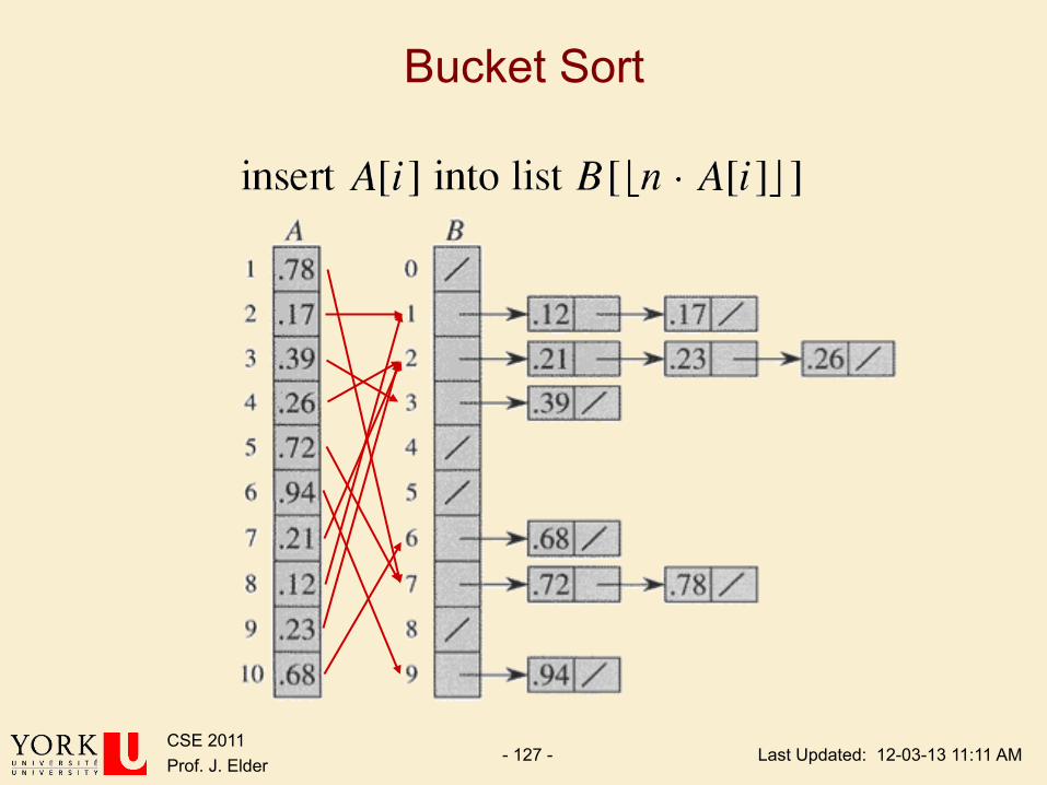
Last Updated: 12-03-13 11:11 AM CSE 2011 Prof. J. Elder - 127 -
Bucket Sort
Last Updated: 12-03-13 11:11 AM CSE 2011 Prof. J. Elder - 128 -
Loop Invariants
Ø Loop 1 q The first i-1 keys have been correctly placed into buckets of
width 1/n.
Ø Loop 2 q The keys within each of the first i-1 buckets have been correctly
stable-sorted.
Last Updated: 12-03-13 11:11 AM CSE 2011 Prof. J. Elder - 129 -
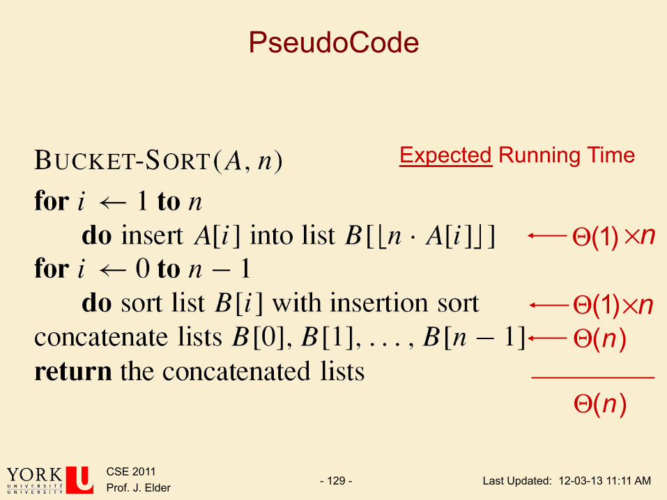
PseudoCode
(1)Θ
(1)Θ( )nΘ
n×
( )nΘ
Expected Running Time
n×
Last Updated: 12-03-13 11:11 AM CSE 2011 Prof. J. Elder - 130 -
Sorting Algorithms Ø Comparison Sorting
q Selection Sort
q Bubble Sort
q Insertion Sort
q Merge Sort
q Heap Sort
q Quick Sort
Ø Linear Sorting q Counting Sort
q Radix Sort
q Bucket Sort

Last Updated: 12-03-13 11:11 AM CSE 2011 Prof. J. Elder - 131 -
Sorting: Learning Outcomes Ø You should be able to:
q Explain the difference between comparison sorts and linear sorting methods
q Identify situations when linear sorting methods can be applied and know why
q Select a sorting method that is well-suited for a specific application.
q Explain what is meant by sorting in place and stable sorting
q State a tight bound on the problem of comparison sorting, and explain why no algorithm can do better.
q Explain and/or code any of the sorting algorithms we have covered, and state their asymptotic run times.