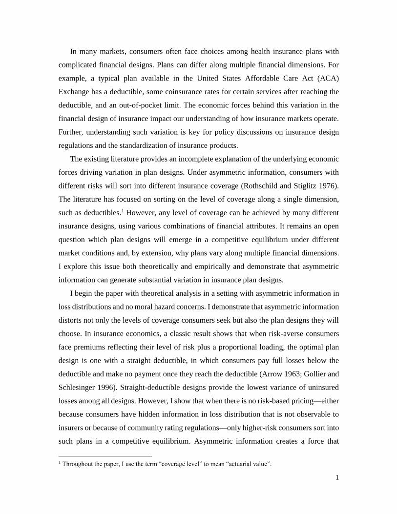
Sorting on Plan Design:

Theory and Evidence from the Affordable Care Act

Chenyuan Liu*

2 March 2021

Latest Version Available Here

Abstract

This paper explores both theoretically and empirically the implications of allowing

multiple cost-sharing attributes for the functioning of health insurance markets. I

characterize a competitive equilibrium under asymmetric information where individuals

with different health risks demand plans with different designs, generating plan variation

even when the coverage level is regulated. Analyzing data from the ACA Exchange, I find

that cost-sharing variations within coverage tiers create significant differences in the risk

protection to consumers. Further, consumers sort by health status in ways consistent with

the theoretical predictions. I discuss how these insights can inform discussions around the

standardization of insurance plans. JEL Codes: D82, G22, I13.

__________________________________ *Department of Economics, School of Economics and Management, Tsinghua University (e-mail:

liuchy3@sem.tsinghua.edu.cn). I thank my adviser Justin Sydnor for his guidance throughout the

development of the paper. For their comments and suggestions, I also thank Naoki Aizawa, Daniel

Bauer, Thomas DeLeire, Yu Ding, Ben Handel, Ty Leverty, David Molitor, John Mullahy, Margie

Rosenberg, Casey Rothschild, Joan Schmit, Mark Shepard, Alan Sorensen, and various seminar

participants. Financial support from the Geneva Association is gratefully acknowledged.

1

In many markets, consumers often face choices among health insurance plans with

complicated financial designs. Plans can differ along multiple financial dimensions. For

example, a typical plan available in the United States Affordable Care Act (ACA)

Exchange has a deductible, some coinsurance rates for certain services after reaching the

deductible, and an out-of-pocket limit. The economic forces behind this variation in the

financial design of insurance impact our understanding of how insurance markets operate.

Further, understanding such variation is key for policy discussions on insurance design

regulations and the standardization of insurance products.

The existing literature provides an incomplete explanation of the underlying economic

forces driving variation in plan designs. Under asymmetric information, consumers with

different risks will sort into different insurance coverage (Rothschild and Stiglitz 1976).

The literature has focused on sorting on the level of coverage along a single dimension,

such as deductibles.1 However, any level of coverage can be achieved by many different

insurance designs, using various combinations of financial attributes. It remains an open

question which plan designs will emerge in a competitive equilibrium under different

market conditions and, by extension, why plans vary along multiple financial dimensions.

I explore this issue both theoretically and empirically and demonstrate that asymmetric

information can generate substantial variation in insurance plan designs.

I begin the paper with theoretical analysis in a setting with asymmetric information in

loss distributions and no moral hazard concerns. I demonstrate that asymmetric information

distorts not only the levels of coverage consumers seek but also the plan designs they will

choose. In insurance economics, a classic result shows that when risk-averse consumers

face premiums reflecting their level of risk plus a proportional loading, the optimal plan

design is one with a straight deductible, in which consumers pay full losses below the

deductible and make no payment once they reach the deductible (Arrow 1963; Gollier and

Schlesinger 1996). Straight-deductible designs provide the lowest variance of uninsured

losses among all designs. However, I show that when there is no risk-based pricing—either

because consumers have hidden information in loss distribution that is not observable to

insurers or because of community rating regulations—only higher-risk consumers sort into

such plans in a competitive equilibrium. Asymmetric information creates a force that

1 Throughout the paper, I use the term “coverage level” to mean “actuarial value”.

2

pushes lower-risk consumers to choose plan designs with more coverage for smaller losses

(in the form of coinsurance and lower deductible) while forgoing coverage on larger losses

(in the form of higher out-of-pocket limits).2

Using formal proofs and numeric simulation, I demonstrate that this theoretical

prediction holds both in an unregulated competitive separating equilibrium and in regulated

markets with perfect risk adjustment. In a competitive market, plan prices reflect the cost

of consumers who actually enroll. In such environments, lower-risk consumers want

insurance coverage but also want a plan that higher-risk consumers find unattractive. Plan

designs that offer relatively strong coverage for smaller losses but high out-of-pocket limits

strike this balance for lower-risk consumers. Under perfect risk adjustment, plan prices

reflect the average cost of coverage under that plan for the full population. In this market,

lower-risk consumers cross-subsidize higher-risk consumers and face prices reflecting

market-average risk levels. Lower-risk consumers generally want plans covering more of

their own losses. Given a fixed premium level, a plan offering more coverage for smaller

losses and less coverage for larger losses gives lower-risk consumers more coverage than

a straight-deductible plan.

The theoretical model is a natural extension of the classic model of Arrow (1963) and

Rothschild and Stiglitz (1976). The model extends Arrow (1963) by allowing for

asymmetric information in loss distributions, and it extends Rothschild and Stiglitz (1976)

by allowing for multiple loss states. While Arrow illustrate the first best plan for multiple

loss states should have a straight-deductible design, my model shows that under

asymmetric information, only the high-risk type sort into such designs. The classic adverse

selection forces in Rothschild and Stiglitz (1976) indicate that the coverage for the lower-

risk type will be distorted downward in a single-loss state scenario. My results characterize

the form of such distortion in a multi-loss-state environment when all designs are available.

In the second part of the paper, I examine the empirical relevance of sorting by plan

design in the ACA Federal Exchange (healthcare.gov), a market with risk-adjustment

regulations. I combine publicly available data on the cost-sharing attributes, premiums,

enrollment, and claims costs for plans launched between 2014 and 2017 in this market. The

2 In my framework, consumers have multiple loss states. Lower (higher) risk types are defined as individuals

having a distribution of losses weighted more heavily toward smaller (larger) losses.

3

ACA Federal Exchange organizes plans into four “metal tiers” based on the level of

coverage they provide for a benchmark average population: Bronze (60%), Silver (70%),

Gold (80%), and Platinum (90%). Within these tiers, insurers have significant latitude in

designing the cost-sharing attributes of their plans in different combinations. I document

that insurers use this latitude to offer plans whose designs vary substantially. For example,

consider the Gold tier, where plans should cover around 80% of costs for the benchmark

average population. I find that, on average, a consumer shopping for plans in this tier face

options with out-of-pocket limits varying by more than $2,000 within a county. This

variation in plan designs within a metal tier is stable over time in the data, with no clear

trends toward more plans with higher out-of-pocket limits or toward straight-deductible

designs. Further, I find that the variation in plan designs is widespread among counties and

insurers.

The variation in financial attributes translates to economically meaningful differences

in the risk protection provided by different plans in the same coverage tier. I quantify the

design variation across plans by calculating the expected utility of choosing each plan for

an individual with a market-average distribution of health risk and a moderate degree of

risk aversion. For such an individual, the straight-deductible plan offers the best risk

protection. Sorting into the other plans available in each tier can have utility costs

equivalent to as much as $1,000 per year.

Variation in plan design creates room for sorting by risk type in the ACA market. My

theoretical model predicts that plans with straight-deductible designs will be attractive to

those with average to above-average risk but will be unattractive for lower-risk consumers.

Using plan-level claims costs and insurer-level risk transfers collected from the Uniform

Rate Review data set, I find that within a metal tier, the straight-deductible plans are chosen

by individuals with significantly larger ex-ante risk scores and ex-post medical expenditure.

My theoretical prediction that consumers will sort by risk level into different plan designs

is reflected in these measures.

In the absence of risk adjustment, straight-deductible plans attracting higher-cost

enrollees would be expected to put pressure on the premiums of those plans. However, I

find that premiums are similar for different plan designs in the same metal tier, suggesting

that the risk adjustment scheme and pricing regulations in the ACA Exchange blunt the

4

pass-through of these selection differences to consumers. Ultimately, the patterns of sorting

by risk type help explain why a wide range of plan designs can emerge in this market, while

the effectiveness of the risk-adjustment scheme helps explain why the market does not

converge to the designs that attract lower-risk consumers.

The theory and empirical analysis presented here highlight how asymmetric

information in risk types can explain the variation in plan designs. However, moral hazard

is another rationale for the existence of non-straight-deductible plans. Theoretical research

has shown that moral hazard can affect the optimal plan design, changing either the

deductible level or the form of coverage (Zeckhauser 1970). Although models with moral

hazard can help explain why plan designs are complex, they offer no ready explanation for

the simultaneous existence of different plan designs. Empirically, my results using risk

scores illustrate that the expenditure differences within an ACA coverage tier are mainly

driven by selection and cannot be explained by moral hazard alone. Interesting dynamics

might be at play when people have asymmetric information about their moral hazard

responses. Those considerations are outside the scope of this paper but could be a valuable

direction for future research.

In the last part of the paper, I explore the implications of variation in plan designs for

market efficiency and regulation. The analysis is motivated by the fact that many countries

are moving towards standardizing health insurance plan designs. For example, in

Netherland, only straight-deductible plans are allowed, while in the California State

Exchange, only standardized non-straight-deductible designs are allowed. To evaluate the

implication of such regulations, I construct realistic distributions of health risks derived

from Truven MarketScan data and use levels of risk aversion estimated in the literature.3 I

then simulate the plans chosen by each risk type when all plans are available in the market,

or when only straight-deductible plans are available. Finally, I calculate the difference in

market efficiency between these two environments.4

I find that the effects of regulating away plan design variation within coverage tiers on

efficiency depend on the underlying market conditions. In a market with perfect risk

3 I use the k-means clustering method to group people based on age, gender, prior expenditure, and pre-

existing conditions. Then I estimate separate spending distributions within these groups. 4 Market efficiency is defined as each consumer’s willingness to pay for the chosen plan and the cost to

insurers to provide that plan, weighted by each consumers’ population size.

5

adjustment, the existence of plan-design variation has a relatively small and ambiguous

impact on market efficiency. Under risk adjustment, lower-risk consumers are inefficiently

under-insured because they respond to market-average prices. For a given price, plans with

non-straight-deductible designs provide more insurance to lower-risk consumers. This

benefit can help offset consumers’ inefficiently low levels of coverage. On the margin,

however, consumers’ decisions may be inefficient because the marginal price they pay for

the additional coverage under these designs may be below the marginal cost of providing

it to them. Ultimately, the overall impact of restricting to straight-deductible plans depends

on the relative importance of the two effects and is ambiguous in risk-adjusted markets.

In unregulated competitive markets, however, plan design variation—specifically, the

existence of plans with low deductibles and high out-of-pocket limits—helps sustain a

more efficient separating equilibrium. When people can sort along only one dimension of

cost-sharing (i.e., deductibles), lower-risk consumers end up sacrificing substantially more

coverage to avoid pooling with higher-risk individuals and may drop out of the market

completely.

To quantify the potential benefits of regulating plan designs in the ACA market, I use

a multinomial logit model to simulate a counterfactual scenario where the actual exchange

plans are replaced with straight-deductible plans that carry the same premium. Consistent

with my general simulations for markets with risk adjustments, I estimate that overall

efficiency for the ACA would be only slightly higher ($10 per person per year) with

regulated plan designs. I also extend the model to allow for the possibility that some

consumers make mistakes when selecting plans, which has been shown to be an issue in

health insurance choice in other settings (e.g., Abaluck and Gruber 2011, 2019; Bhargava,

Lowenstein and Sydnor 2017). Plans with high out-of-pocket limits create the possibility

of a costly mistake for higher-risk consumers, who are disproportionately adversely

affected by such plans. I show that the efficiency benefits of regulating plan designs in the

ACA Exchange are significantly higher if a moderate share of consumers makes plan-

choice mistakes.

Related Literature

The paper builds on and offers new insights into the literature on insurance coverage

distortions under asymmetric information. This paper's theoretical framework follows

6

Rothschild and Stiglitz (1976) and adds to subsequent works on endogenous contract

design under asymmetric information (Crocker and Snow 2011; Hendren 2013; Handel,

Hendel, and Whinston 2015; Veiga and Weyl 2016; Azevedo and Gottlieb 2017). A stream

of this theoretical literature model individual heterogeneity along one dimension. For

example, individuals have a binary loss state (Rothschild and Stiglitz 1976; Hendren 2013)

or differ by their willingness to pay for one contract (Einav, Finkelstein and Cullen, 2010;

Handel, Hendel, and Whinston 2015). Unlike this approach, I allow private information on

multiple loss states and model consumer choices when they face contracts with multiple

cost-sharing attributes. Thus, the model informs the mechanism driving complex cost-

sharing designs available in health insurance markets and help explain endogenous cost-

sharing designs.5

My model also adds to the applied theory literature on contract design under risk

adjustment (Frank, Glazer and McGuire 2000; Glazer and McGuire 2000, 2002; Ellis and

McGuire 2006; Jack 2006). While previous works focus on a risk-adjusted environment

where individuals differ in the likelihood of incurring different diseases, I characterize

individual behaviors when they differ in the loss distribution of multiple loss states. My

model shows that selection along multiple cost-sharing attributes exists in a market with

perfect risk adjustment.

The paper also adds to a growing empirical literature documenting adverse selection

and contract screening in health insurance markets. Previous works document a range of

consumer selection and insurer screening channels, including coverage levels (see Breyer,

Bundorf, and Pauly (2011) for a review), managed care plans (see Glied (2000) for a

review), provider networks (Shepard 2016), drug formulary and covered benefits (Lavetti

and Simon 2014; Carey 2016; Geruso, Layton, and Prinz 2019), and advertisement

(Aizawa and Kim 2018). This paper presents empirical evidence of a new channel of

selection in the health insurance market: sorting by multidimensional cost-sharing

attributes. This channel is different from selection coverage levels or premiums,

representing a vertical differentiation among plans. Instead, the paper documents

5 For example, Decarolis and Guglielmo (2017) documented that 5-star Medicare Part C plans increase OOP

limits and decrease deductible levels in the face of the pressure of worsening risk pools. Under my framework,

this is consistent with non-straight-deductible plans being more attractive to healthy types.

7

sorting within a coverage tier: In the ACA Exchange, sorting happens among plans

differing along multiple cost-sharing attributes but with equal premiums, a unique pattern

not documented before. Moreover, in contrast to the above works' findings that risk-

adjustment schemes are imperfect, I find that the ACA risk-adjustment scheme is effective

at flattening the effect of adverse selection on premiums across plans with different

financial designs.

Finally, the research presented in this paper identifies an understudied mechanism

shaping the complex financial plan designs in insurance markets. Previous studies find that

moral hazard (Pauly 1968; Zeckhauser 1970; Einav et al. 2013), nonlinear loading factors

or risk-averse insurers (Raviv 1979), background risk (Doherty and Schlesinger 1983), and

liquidity constraints (Ericson and Sydnor 2018) can lead people to select into these types

of plan designs. This paper illustrates how asymmetric information can also rationalize

complex plan design variation. I find empirical evidence that different risk types sort on

different plan designs, suggesting that this mechanism can play a role in rationalizing

observed plan offerings and sorting in the ACA Exchange.

The rest of the paper is organized as follows: In Section 2, I lay out the conceptual

framework and derive the conditions leading to design distortion. In Section 3, I examine

the issue empirically using the ACA Federal Exchange data. In Section 4, I discuss the

implications for regulating plan designs. The final section concludes.

2 Conceptual Framework of Optimal Plan Design

Arrow (1963) began a large literature exploring the optimal design of insurance plans

in the absence of moral hazard concerns. A classic result from this literature is that straight-

deductible plans offer optimal insurance (Arrow 1963; Gollier and Schlesinger 1996).

Under such plans, consumers pay full losses out-of-pocket before the deductible level and

get full insurance once they reach the deductible level. However, whether the straight-

deductible design remains optimal hinges on the assumption that all plans are priced based

on individual risk. With heterogeneous risk types and asymmetric information or

community rating, theorems establishing the optimality of straight deductible plans do not

apply. I show that in general, higher-risk consumers will sort into straight-deductible

8

designs while lower-risk consumers choose designs that allow them to trade more coverage

for smaller losses with less coverage for worst-case events.

2.1 Model Setup

Setting. Individual 𝑖 faces uncertainty. I model this uncertainty via a set of finite states 𝑆

with generic element 𝑠. The realization of 𝑠 ∈ 𝑆 is uncertain, with state 𝑠 obtaining with

probability 𝑓𝑠𝑖 for individual 𝑖. Each state 𝑠 is associated with a loss 𝑥𝑠. Individuals differ

from each other by the probabilities of experiencing each loss state. Let 𝑓𝑠𝑖 denote the

probability of individual 𝑖 being in state 𝑠 . 6 This model generalizes the binary loss

environment by allowing individuals to have more than one possible loss amount.

I consider a general state-dependent insurance plan that captures the wide range of

potentially complex plan design consumers could desire. Specifically, an insurance plan is

defined as a function 𝒍: 𝑠 → 𝑅+ . I also define 𝑙𝑠 ≡ 𝑙(𝑠) as the value of the function

evaluated at 𝑠, so 𝑙𝑠 represents the insurer indemnity in state 𝑠. The insurance payment 𝑙𝑠

satisfies the condition 0 ≤ 𝑙𝑠 ≤ 𝑥𝑠, which implies the insurance payment is non-negative

and no larger than the size of the loss. The expected insurer indemnity for individual 𝑖 is

∑ 𝑓𝑠𝑖𝑙𝑠𝑠 .

The financial outcome (consumption) after insurance in each loss state is 𝑤𝑖 − 𝑥𝑠 +

𝑙𝑠 − 𝑝(𝒍) , where 𝑤𝑖 is the non-stochastic initial wealth level and 𝑝(𝒍) represents the

premium of plan 𝒍. In the baseline model, I assume individuals have a concave utility

function 𝑢𝑖 over the financial outcome of each loss state: 𝑢𝑖′ > 0, 𝑢𝑖

′′ < 0. Consumers are

offered a menu of contracts 𝐶 and choose the plan maximizing their expected utility:

𝑚𝑎𝑥𝒍∈𝐶

∑ 𝑢𝑖(𝑤𝑖 − 𝑥𝑠 + 𝑙𝑠𝑠

− 𝑝(𝒍))𝑓𝑠𝑖. (1)

In the following analysis, I consider the competitive equilibrium under three different

market conditions: symmetric information (risk-based pricing), asymmetric information

(community rating), and asymmetric information (community rating) with risk adjustment.

Under each case, the menu of plans (𝐶) faced by individuals and the premium of each plan

𝑝(𝒍) will be different.

Case 1. Symmetric Information/Risk-Based Pricing

6 In this setup, I consider discretely distributed loss states. The setting and proofs can be extended to a

scenario where losses are continuously distributed.

9

I first show that if there is a single risk type in the market (or, equivalently, if risk types

are fully known and can be priced), and if all contracts have equal loading, then the optimal

plan has a straight deductible design. This is a specific case of the classic results of Arrow

(1963) and Gollier and Schlesinger (1996) by assuming premiums is a linear function of

expected covered losses.

For this single-risk-type case, I drop subscript 𝑖 for simplicity of exposition. Assume

perfectly competitive insurers set premiums as a linear function of the expected covered

expenditure: 𝑝(𝒍) = 𝜃 ∑ 𝑓𝑠𝑙𝑠𝑠 + 𝑐, where 𝜃 ≥ 1 is a proportional loading factor, and 𝑐 ≥

0 is a fixed loading.7 The premium of insurance plan 𝒍 is:

𝑝(𝒍) = 𝜃 ∑ 𝑓𝑠𝑙𝑠𝑠

+ 𝑐.

Suppose further that all possible insurance contracts are available and priced this way.

Proposition 1 states the form of optimal insurance in this case:

Proposition 1. [Arrow: The Optimality of Straight-Deductible Plans under Risk-based

Pricing] Suppose there is a single risk type in the market, and the premium is a linear

function of the expected covered expenditure. For any fixed loading factors, the expected-

utility-maximizing contract is a straight deductible plan.

Proof: See Appendix A.

One way to see the optimal insurance is to consider the first-order-condition:

𝑢𝑠′ ≤ 𝜃 ∑ 𝑢𝜏

′ 𝑓𝜏𝜏

, ∀𝑠, (2)

with equality if 𝑙𝑠 > 0.

The left-hand side represents the marginal benefit of the reduction in out-of-pocket

costs, and the right-hand-side represents the marginal costs (via the effects on premium) of

increasing coverage for that loss state. The left-hand side is a decreasing function with

regard to 𝑙𝑠 because 𝑢𝑠′′ < 0 for all loss states (consumers are risk averse). When 𝜃 = 1,

the left-hand side can be the same for all loss states. Essentially, individuals get full

insurance. When 𝜃 > 1, 𝑢𝑠′ < 𝜃 ∑ 𝑢𝜏

′ 𝑓𝜏𝜏 for small loss states and thus 𝑙𝑠 = 0 (no coverage

for smaller losses). When 𝑥𝑠 is large enough, 𝑙𝑠 > 0 and 𝑢𝑠′ is the same across these loss

states. This implies that for these loss states the consumption, 𝑤 − 𝑥𝑠 + 𝑙𝑠 − 𝑝(𝒍), is

7 The loadings capture costs of operation for the competitive insurers.

10

constant. As a result, consumers pay a fixed deductible ( 𝑥𝑠 − 𝑙𝑠) in these states. In

summary, when 𝜃 > 1, the optimal insurance is in the form of no coverage for small losses,

and a deductible once the loss is large enough. Intuitively, a straight-deductible plan

smooths consumption for large losses and has the lowest variance in uninsured risk,

holding fixed the premium. The deductible level is determined by the loading factor and

risk aversion level.

Case 2. Asymmetric Information/Community Rating

Now consider the case where there are two risk types (𝐿 and 𝐻) equally distributed in

the market. Their respective probabilities of being in state 𝑠 are 𝑓𝑠𝐿 and 𝑓𝑠

𝐻, and the utility

functions are 𝑢𝐿 and 𝑢𝐻 respectively. Let 𝑙𝐿𝑠∗ and 𝑙𝐻𝑠

∗ denote the utility-maximizing

insurance payment in state 𝑠 for each type. There is asymmetric information in the market:

insurers cannot distinguish 𝐿 from 𝐻 ex-ante, or they could not charge different premiums

for the same plan because of community rating regulations.

Analogous to Rothschild and Stiglitz (1976), consider a potential separating

equilibrium where one risk type (𝐻) gets the optimal contract under full information, and

the other type (𝐿) distorts their coverage to prevent the higher-risk type from pooling with

them.8 A necessary condition for such an equilibrium requires no deviation for the 𝐻 type.

This suggests that in such an equilibrium, the contracts 𝐿 choose from have to give 𝐻 no

more expected utility than the first-best plan chosen by 𝐻 (incentive compatibility).

I also look at equilibria in which premiums are a mechanical function of the expected

covered losses given who sorts into that plan. Examples of such equilibria include

Rothschild and Stiglitz (1976), and Azevedo and Gottlieb (2017). This model rules out

equilibrium concepts with cross-subsidization among plans (as in Spence 1978). 9 Note the

similarity and difference of the problem faced by the low-risk type between this case and

Case 1. In both cases, plans are priced based on expected covered loss of 𝐿. However, in

Case 1, 𝐿 can choose from all possible contracts; In Case 2, 𝐿 can only choose from

incentive compatible contracts. These contracts prevent 𝐻 from deviating from their

equilibrium plan.

8 Here, the 𝐻 and 𝐿 types are defined such that the incentive compatibility constraint for the 𝐻 type is

constrained while the incentive compatibility constraint for 𝐿 is slack. The exercise is to characterize the

property of such an equilibrium if it exists. 9 In Appendix A, I show a similar proposition which relaxes the premium requirement.

11

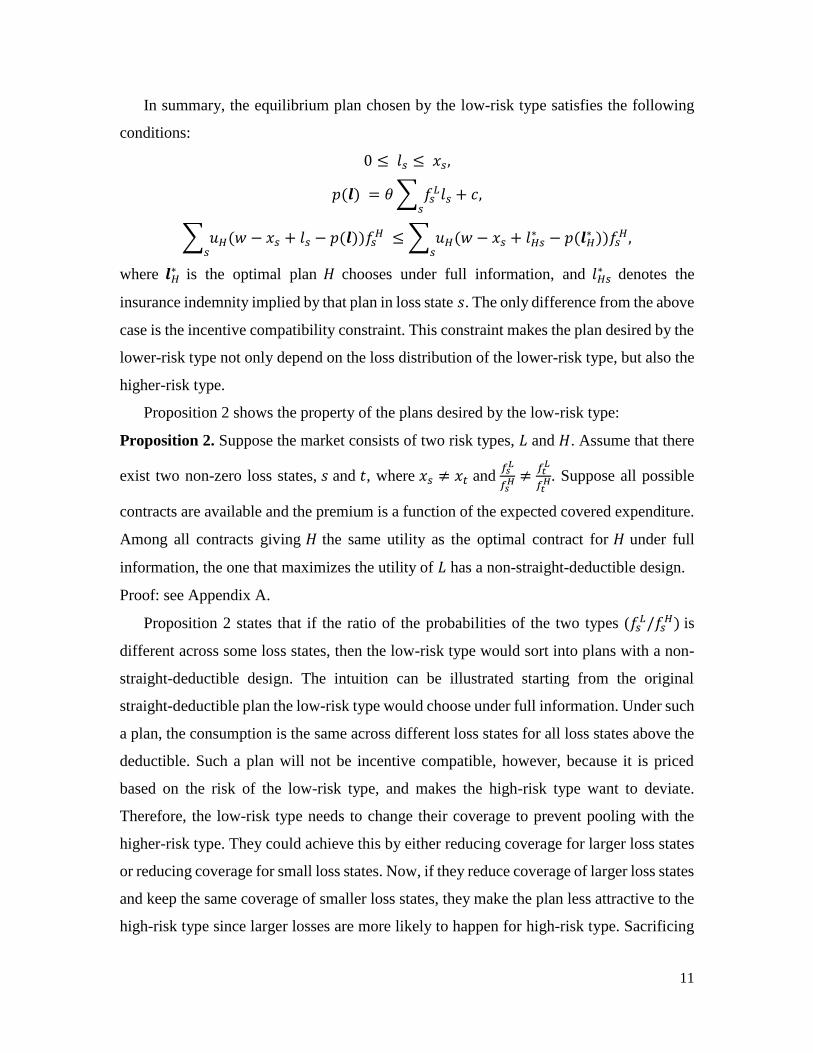
In summary, the equilibrium plan chosen by the low-risk type satisfies the following

conditions:

0 ≤ 𝑙𝑠 ≤ 𝑥𝑠,

𝑝(𝒍) = 𝜃 ∑ 𝑓𝑠𝐿𝑙𝑠

𝑠+ 𝑐,

∑ 𝑢𝐻(𝑤 − 𝑥𝑠 + 𝑙𝑠𝑠

− 𝑝(𝒍))𝑓𝑠𝐻 ≤ ∑ 𝑢𝐻(𝑤 − 𝑥𝑠 + 𝑙𝐻𝑠

∗

𝑠− 𝑝(𝒍𝐻

∗ ))𝑓𝑠𝐻,

where 𝒍𝐻∗ is the optimal plan 𝐻 chooses under full information, and 𝑙𝐻𝑠

∗ denotes the

insurance indemnity implied by that plan in loss state 𝑠. The only difference from the above

case is the incentive compatibility constraint. This constraint makes the plan desired by the

lower-risk type not only depend on the loss distribution of the lower-risk type, but also the

higher-risk type.

Proposition 2 shows the property of the plans desired by the low-risk type:

Proposition 2. Suppose the market consists of two risk types, 𝐿 and 𝐻. Assume that there

exist two non-zero loss states, 𝑠 and 𝑡, where 𝑥𝑠 ≠ 𝑥𝑡 and 𝑓𝑠

𝐿

𝑓𝑠𝐻 ≠

𝑓𝑡𝐿

𝑓𝑡𝐻. Suppose all possible

contracts are available and the premium is a function of the expected covered expenditure.

Among all contracts giving 𝐻 the same utility as the optimal contract for 𝐻 under full

information, the one that maximizes the utility of 𝐿 has a non-straight-deductible design.

Proof: see Appendix A.

Proposition 2 states that if the ratio of the probabilities of the two types (𝑓𝑠𝐿/𝑓𝑠

𝐻) is

different across some loss states, then the low-risk type would sort into plans with a non-

straight-deductible design. The intuition can be illustrated starting from the original

straight-deductible plan the low-risk type would choose under full information. Under such

a plan, the consumption is the same across different loss states for all loss states above the

deductible. Such a plan will not be incentive compatible, however, because it is priced

based on the risk of the low-risk type, and makes the high-risk type want to deviate.

Therefore, the low-risk type needs to change their coverage to prevent pooling with the

higher-risk type. They could achieve this by either reducing coverage for larger loss states

or reducing coverage for small loss states. Now, if they reduce coverage of larger loss states

and keep the same coverage of smaller loss states, they make the plan less attractive to the

high-risk type since larger losses are more likely to happen for high-risk type. Sacrificing

12

coverage for large losses and transferring to coverage for small losses is less problematic

for the low-risk type, though, since most of their losses are likely to be small.

Case 3. Asymmetric Information/Community Rating with Perfect Risk Adjustment

In many markets, regulators impose risk adjustment regulations to flatten premium

differences among different plans and to remove screening incentives for insurers. Such

regulation enforces a cross-subsidization from lower-risk type to higher-risk type. I

consider a market with perfect risk adjustment where the premium reflects the market

average risk and is a linear function of the expected costs that would be obtained if all risk

types enroll in the plan.10 This approximates the regulatory environment in many US health

insurance markets, including Medicare Advantage, Medicare Part D, and the ACA

Exchange, and will be relevant for the empirical analyses in Section 3.11

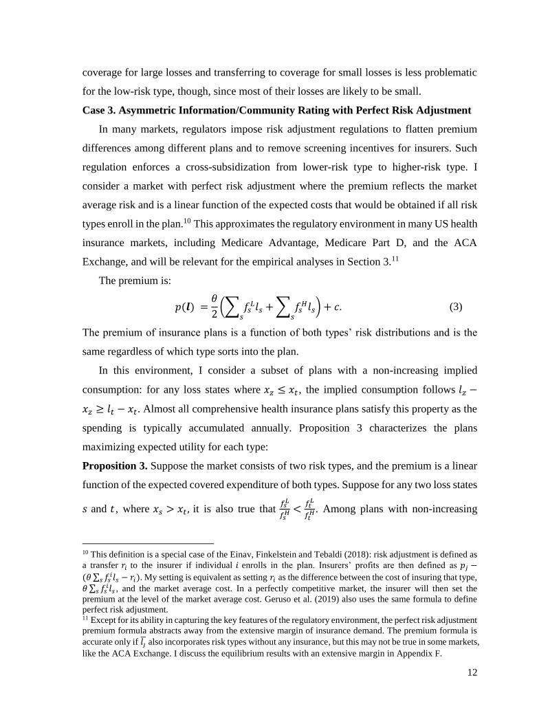
The premium is:

𝑝(𝒍) =𝜃

2(∑ 𝑓𝑠

𝐿𝑙𝑠𝑠

+ ∑ 𝑓𝑠𝐻𝑙𝑠

𝑠) + 𝑐. (3)

The premium of insurance plans is a function of both types’ risk distributions and is the

same regardless of which type sorts into the plan.

In this environment, I consider a subset of plans with a non-increasing implied

consumption: for any loss states where 𝑥𝑧 ≤ 𝑥𝑡 , the implied consumption follows 𝑙𝑧 −

𝑥𝑧 ≥ 𝑙𝑡 − 𝑥𝑡. Almost all comprehensive health insurance plans satisfy this property as the

spending is typically accumulated annually. Proposition 3 characterizes the plans

maximizing expected utility for each type:

Proposition 3. Suppose the market consists of two risk types, and the premium is a linear

function of the expected covered expenditure of both types. Suppose for any two loss states

𝑠 and 𝑡 , where 𝑥𝑠 > 𝑥𝑡 , it is also true that 𝑓𝑠

𝐿

𝑓𝑠𝐻 <

𝑓𝑡𝐿

𝑓𝑡𝐻 . Among plans with non-increasing

10 This definition is a special case of the Einav, Finkelstein and Tebaldi (2018): risk adjustment is defined as

a transfer 𝑟𝑖 to the insurer if individual 𝑖 enrolls in the plan. Insurers’ profits are then defined as 𝑝𝑗 −

(𝜃 ∑ 𝑓𝑠𝑖𝑙𝑠𝑠 − 𝑟𝑖). My setting is equivalent as setting 𝑟𝑖 as the difference between the cost of insuring that type,

𝜃 ∑ 𝑓𝑠𝑖𝑙𝑠𝑠 , and the market average cost. In a perfectly competitive market, the insurer will then set the

premium at the level of the market average cost. Geruso et al. (2019) also uses the same formula to define

perfect risk adjustment. 11 Except for its ability in capturing the key features of the regulatory environment, the perfect risk adjustment

premium formula abstracts away from the extensive margin of insurance demand. The premium formula is

accurate only if 𝑙�̅� also incorporates risk types without any insurance, but this may not be true in some markets,

like the ACA Exchange. I discuss the equilibrium results with an extensive margin in Appendix F.

13

implied consumption, the higher-risk type will sort into a straight-deductible plan, but not

the lower-risk type.

Proof: see Appendix A.

Under perfect risk adjustment, the premiums are effectively “shared” between the two

types. The marginal cost of reducing out-of-pocket spending does not only depend on their

own spending, but also the spending of the other type. Ideally, both types want to have the

premium covering more of their own spending than the spending of the other type. Holding

fixed a premium level, the straight-deductible plans give the low-risk type the lowest

expected coverage relative to all other possible designs. This is because straight-deductible

designs offer full coverage for larger losses, and it is that coverage that gets reflected in the

premium for these plans. High-loss states though, are dominated by higher-risk individuals.

Alternatively, a plan that gives up coverage of large losses for coinsurance rates of small

losses is more beneficial to the low-risk type because they are more likely to incur small

losses, and thus get more expected coverage from such a plan. This suggests that the plan

desired by the low-risk type has coinsurance rates (if not full coverage) for smaller losses,

and smaller or even no coverage for large losses. For the high-risk type, the opposite is true.

A straight-deductible plan provides them with higher consumption in larger loss states, and

are thus is chosen optimally in a competitive equilibrium.

Note on the definition of risk types. In Proposition 2 and 3, 𝐻 and 𝐿 are defined based on

the ratio of the probability density function. In Proposition 2, the implicit requirement is

that the incentive compatibility constraint is slack for 𝐻 and constrained for 𝐿. Under this

condition, and the condition that there exist two loss states where the ratio of the probability

density function is different, 𝐿 prefers non-straight-deductible plan over a straight-

deductible design. In proposition 3, the condition under which sorting happens is that 𝑓𝑠

𝐿

𝑓𝑠𝐻 <

𝑓𝑡𝐿

𝑓𝑡𝐻 for any 𝑥𝑠 > 𝑥𝑡. Under this condition, the expected loss is smaller for 𝐿 than 𝐻.

Corollary 1. Suppose the market consists of two risk types, 𝐿 and 𝐻. Suppose for any two

loss states 𝑠 and 𝑡, where 𝑥𝑠 > 𝑥𝑡 , it is also true that 𝑓𝑠

𝐿

𝑓𝑠𝐻 <

𝑓𝑡𝐿

𝑓𝑡𝐻. Then 𝐸𝐿(𝑥) < 𝐸𝐻(𝑥).

Proof: see Appendix A.

In both Case 2 and Case 3, what matters is the ratio of the probability density function.

Intuitively, the probability density function ratio represents the slope of the iso-profit line

14

in the consumption space. A difference in the slope implies 𝐿 is better off by differentiating

consumption in the two loss states, a deviation from the straight-deductible plan. Appendix

Figure 1 provides a graphical illustration for the intuition.

2.2 Model Extensions

In this section, I discuss the robustness of the pattern with more than two risk types,

heterogeneity in risk aversion, and the existence of moral hazard responses.

2.2.1 More than Two Risk Types

The sorting on plan design mechanism can be easily extended to a market with more

than two discrete risk types. The intuition is similar: Non-straight-deductible designs

provide more coverage in loss states where the lower-risk types are more likely to

experience relative to the higher-risk types. Appendix Figure 2 shows a numeric example

with 15 risk distributions constructed from the Truven MarketScan data (I discuss the detail

on how I construct these distributions in Section 2.3.1 and Appendix C). Under perfect risk

adjustment, the types choosing the straight-deductible design have significantly more

probability mass on the right tail of their loss distribution.

2.2.2 Heterogeneity in Risk Aversion

A growing literature documents the existence of advantageous selection. One potential

explanation for it may be heterogeneity in risk aversion, or more specifically, risk aversion

being negatively correlated to risk types (Finkelstein and McGarry 2006; Fang, Keane, and

Silverman 2008). In my model, adding heterogeneity in risk aversion does not change the

basic sorting pattern where different risk types sort into different designs in equilibrium.

The proofs of Proposition 2 and 3 incorporate cases where the two risk types have different

risk aversion. The sorting pattern persists as long as both types are risk averse.12 Intuitively,

if the low risk types are more risk averse, in equilibrium, they will want more insurance

coverage in the form of lower coinsurance rate and lower deductible levels. But as long as

there is a difference in the ratio of the loss probability across loss states between the two

12 Proposition 2 relies on the assumption that at least one risk type has a binding incentive compatibility

constraint, which depend on the parametric form of the utility function.

15

types, then the low risk types always have an incentive to deviate from the straight-

deductible design.

2.2.3 Moral Hazard

Literature shows the optimality of straight-deductible plan may not hold when there is

ex-post moral hazard (Zeckhauser 1970). The empirical literature examining moral hazard

in health insurance plans typically leverages the variation across different coverage levels

(Einav et al. 2013; Brot-Goldberg et al. 2018). There are limited research modeling moral

hazard responses when consumers face options with rich variations in financial designs

within a coverage or premium level, the focus of this paper. In this section, I modify my

model to allow ex-post moral hazard responses in consumers’ utility function and illustrate

the robustness of the sorting pattern when there is both moral hazard and adverse selection.

I follow the framework introduced by Einav et al. (2013) in modeling moral hazard.

The model assumes that after the health risk is realized, individuals get utility from both

the financial outcome and the level of medical expenditure. I assume that consumers over

spend by 20% of the health shock when moving from no insurance to full insurance. I also

assume that insurers can perfectly observe the level of ex-post moral hazard responses of

each type, making the information asymmetry only come from ex-ante loss distribution. I

then use the model to simulate the plans chosen by each risk type under different market

conditions. The details of the model are in Appendix B.

There are two key insights from the model. First, under risk-based pricing, the plans

desired by both types have straight-deductible designs, suggesting that this specific form

of moral hazard responses alone cannot explain the existence of many different designs.

Second, when there are both moral hazard and asymmetric information in the loss

distributions, the plan desired by the higher-risk type has a straight deductible design, and

the plan desired by the lower-risk type has a non-straight-deductible design. These results

suggest that the key prediction of my model, that high-risk sorts into straight-deductible

plans but not the low-risk, holds when there are both moral hazard and asymmetric

information in risk types.

2.3 Illustrative Example

In this section, I present a numerical example illustrating the sorting pattern based on

an empirically realistic set of risk distributions.

16

2.3.1 Setup

The Demand Side. In this simulation, I parameterize the consumer preference using the

constant-absolute-risk-aversion (CARA) utility function. Consumers are risk averse with a

risk-aversion coefficient 𝛾𝑖 > 0 . 13 For the following simulation, I also assume

homogenous risk aversion for the two types and set 𝛾 = 0.0004, which is the mean level of

risk aversion estimated by Handel (2013) for a population of employees selecting among

health insurance plans.

To calculate plans chosen by different risk types, I need information about the ex-ante

medical expenditure distributions. I derive such information using the Truven MarketScan

database, a large claims database for the US employer-sponsored plans. To characterize

heterogeneity in medical expenditure, I use the k-means clustering method to classify

individuals into two groups, based on their age, gender, employment status, pre-existing

conditions (constructed based on diagnosis codes and procedures performed), and medical

expenditure. I then estimate separate spending distributions within each group. The

resulting lower-risk type has an expected risk of $1,843 and a standard deviation of $7,414,

representing 26% population in the sample. The higher risk has an expected risk of $7,537

and a standard deviation of $22,444. The details of the method are in Appendix C.

Appendix Figure C1 shows that the two probability density functions have different shapes:

The low-risk type has greater probability density on smaller losses while the high-risk type

has greater probability density on larger losses.

The Supply Side. For the premium, I assume insurers charge a premium 20% higher

than the claims costs (𝜃 = 1.2).14 I simulate the premiums of each plan, either under no risk

adjustment or perfect risk adjustment. For the no-risk adjustment case, I follow the

equilibrium notion by Azevedo and Gottlieb (2017) to calculate the equilibrium plans

(details are in Appendix A.)

The Choice Set. I consider a choice set with rich variation in the cost-sharing attributes.

I allow for two broad categories of plan designs. The first category of plans has a three-

13 This functional form removes income effects and is used in many prior works modeling insurance choice

(e.g. Handel 2013; Abaluck and Gruber 2019). 14 Regulations adopted as part of the Affordable Care Act require insurers to have at least 80% or 85%

(depending on the size) of their premium used to cover claims costs. When this regulation binds, it implies a

loading factor of around 1.2.

17

arm design with four plan attributes: A deductible, an out-of-pocket-limit (OOP-limit, the

maximum of the out-of-pocket spending per year), a coinsurance rate (the share of medical

expenditure paid by consumers) before the deductible, and a coinsurance rate after the

deductible. To make the simulation tractable, I discretize the contract space and assume the

OOP-limit is no larger than $100,000. The second category consists of constant

coinsurance plans, with a coinsurance rate ranging between zero and one.15 Both full

insurance (in the form of zero constant coinsurance to consumers) and no insurance are in

the choice set.

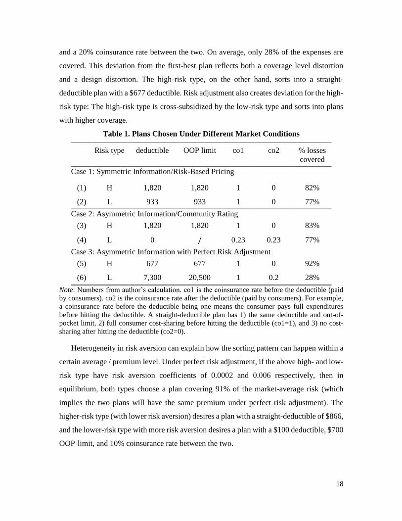
2.3.2 Results

As expected from the analysis above, when there is no asymmetric information and

both types face type-specific premiums, the straight deductible plans are optimal. Table 1

rows (1) and (2) show this result. The low-risk type desires a plan with a $933 straight-

deductible, and the high-risk type desires a plan with an $1820 straight-deductible. Both

are plausible and similar to the plans observed in the employer-sponsored market and the

ACA Exchange. The deductible level is larger than zero (they get less than full insurance)

because there is a positive loading in insurance plans. On average, the high-risk type has

82% of their expenses covered, and the low-risk type has 77% of their expenses covered.

When there is asymmetric information and no risk adjustment, the low-risk type sorts

into a non-straight-deductible design with a constant coinsurance rate (paid by consumers)

of 23%. The plan covers 77% of medical expenditures for the low-risk type at all loss

levels.16 Even though the coverage level is similar to those under perfect information, there

is a large distortion in the design such that the low-risk type is subject to a large variation

in out-of-pocket spending. The high-risk type has no distortion and gets the same straight-

deductible plan they would have chosen under full information.

The design distortion persists when there is perfect risk adjustment. The low-risk type

still sorts into a non-straight-deductible design, though the OOP-limit is much smaller. In

this case, the low-risk type sorts into a plan with a $7,300 deductible, a $20,500 OOP-limit,

15 The three-arm design is popular in the ACA Exchange, Medicare Part C and D, and employer sponsored

insurance plans. Traditional Medicare plans are (a variation of) constant coinsurance plans. 16 This extremely high out-of-pocket limit in this example may be driven in part by the CARA utility form,

which ignores income effects.

18

and a 20% coinsurance rate between the two. On average, only 28% of the expenses are

covered. This deviation from the first-best plan reflects both a coverage level distortion

and a design distortion. The high-risk type, on the other hand, sorts into a straight-

deductible plan with a $677 deductible. Risk adjustment also creates deviation for the high-

risk type: The high-risk type is cross-subsidized by the low-risk type and sorts into plans

with higher coverage.

Table 1. Plans Chosen Under Different Market Conditions

Risk type deductible OOP limit co1 co2 % losses

covered

Case 1: Symmetric Information/Risk-Based Pricing

(1) H 1,820 1,820 1 0 82%

(2) L 933 933 1 0 77%

Case 2: Asymmetric Information/Community Rating

(3) H 1,820 1,820 1 0 83%

(4) L 0 / 0.23 0.23 77%

Case 3: Asymmetric Information with Perfect Risk Adjustment

(5) H 677 677 1 0 92%

(6) L 7,300 20,500 1 0.2 28%

Note: Numbers from author’s calculation. co1 is the coinsurance rate before the deductible (paid

by consumers). co2 is the coinsurance rate after the deductible (paid by consumers). For example,

a coinsurance rate before the deductible being one means the consumer pays full expenditures

before hitting the deductible. A straight-deductible plan has 1) the same deductible and out-of-

pocket limit, 2) full consumer cost-sharing before hitting the deductible (co1=1), and 3) no cost-

sharing after hitting the deductible (co2=0).

Heterogeneity in risk aversion can explain how the sorting pattern can happen within a

certain average / premium level. Under perfect risk adjustment, if the above high- and low-

risk type have risk aversion coefficients of 0.0002 and 0.006 respectively, then in

equilibrium, both types choose a plan covering 91% of the market-average risk (which

implies the two plans will have the same premium under perfect risk adjustment). The

higher-risk type (with lower risk aversion) desires a plan with a straight-deductible of $866,

and the lower-risk type with more risk aversion desires a plan with a $100 deductible, $700

OOP-limit, and 10% coinsurance rate between the two.

19

3. Empirical Analysis

In this section, I show evidence that the design sorting pattern plays a significant role

in the current US health insurance market. I use the ACA Exchange data and document

large variation in plan design, with a sizable demand for non-straight-deductible plans. I

then document a sorting pattern into plan designs consistent with the prediction of the

conceptual framework.

3.1 Institutional Background

The Affordable Care Act Exchange (the Exchange henceforth) was launched in 2014.

Private insurers can offer comprehensive health insurance plans, and the federal

government provides subsidy for certain low-income consumers who purchased plans.

Each state can either join the Federal Exchange or establish its state exchange.17 I focus on

the federally administered Individual Exchange operated via healthcare.gov as it covers

most states (40 states in 2017) and has the following regulations suitable to study the plan

design variation.

The Exchange regulates the actuarial value of plans but leaves insurers with latitude to

offer a range of different plan designs. The Exchange has regulation on the market-average

actuarial value: Plans can only have a population-average AV of around 60%, 70%, 80%,

and 90%, and are labeled as Bronze, Silver, Gold and Platinum plans respectively.18 The

Exchange also requires plans to have an upper limit on out of pocket costs ($7,150 in 2017).

Insurers are otherwise free to offer any cost-sharing attributes. Some state Exchanges

further regulate the plan designs, so I only focus on the Federal Exchange.19

There are also ACA regulations limiting insurers' ability and incentive to do risk

screening. The regulators calculate risk scores for enrollees and transfer money from

insurers with a lower-cost risk pool to insurers with a higher-cost risk pool, to equalize plan

costs across insurers. Further, there is a single risk pool pricing regulation to equalize plan

costs within insurers. The premiums of plans offered by the same insurer will be set based

17 Plans launched in states using healthcare.gov are still subject to each state’s insurance regulation, for

example, the essential health benefits that must be covered by a plan may differ across states. 18 Consumers with income level below a certain level are qualified for cost-sharing reduction variations,

which have a higher AV than standard Silver plan and the same premium. Consumers below 30 are eligible

for Catastrophic plans with minimum coverage. 19 Insurers in Connecticut, District of Columbia, Massachusetts, New York, Oregon, and Vermont must offer

standardized options and can offer a limited number of non-standardized options within a metal tier.

California requires all insurers to offer only standardized plans.

20

on the overall risk pool of that insurer, not the risk of individuals enrolled in each plan.

Third, community rating limits insurers' ability to set premiums based on individual

characteristics. Premiums can only vary by family composition, tobacco user status, and

(partially) by age group. In the following analysis, I provide new evidence on the risk

adjustment scheme in the ACA Exchange and discuss how the perfect risk-adjustment

assumption likely holds along the plan design dimension.

3.2 Data

I use Health Insurance Exchange Public Use Files from 2014 to 2017. This dataset is a

publicly available dataset of the universe of plans launched through healthcare.gov.

Appendix Table 1 shows the states in the sample. I define a unique plan based on the plan

ID administered by CMS, which is a unique combination of state, insurer, network, and

cost-sharing attributes, and also is the level of choice in the menu faced by consumers.20

For each plan, I observe its financial attributes (deductibles, coinsurance rates, copays,

OOP-limits, etc.), premium (which varies at plan-rating area level), and enrollment

numbers in that plan (at plan-state level). I focus on the 2017 year for the main analysis,

but the results are similar for other years.

I use the Uniform Rate Review Data from 2014 to 2017. The dataset contains average

claims costs information (including both insurer payments to providers and the consumer

cost-sharing) at the plan-state level and insurer-state level, as well as risk transfers at

insurer-state level. I discuss these data in more detail in Section 3.4 when I examine the

extent to which there is differential sorting across risk types into different plan designs.

3.3 Analysis of Plan Design Variations in the ACA Market

The market is populated with both straight-deductible and non-straight deductible plans.

Table 2 shows the market share of straight-deductible plans over time. Take the year 2016

as an example. There are around 4,000 unique plans offered in this market. Among them,

13% are straight-deductible plans. In total 9.7 million consumers purchased a plan in this

market, and about 7.6% of them selected a straight-deductible plan.

20 As noted before, each Silver plan has three cost-sharing variations. In almost all cases, the straight-

deductible design is consistent across the standard plans and the cost-sharing variations: either all variations

have a straight deductible design, or none of them have a straight-deductible design. In such analyses, I count

a Silver plan along with its variations as one plan, because the enrollment and claims costs are at plan level,

not plan-variation level.

21

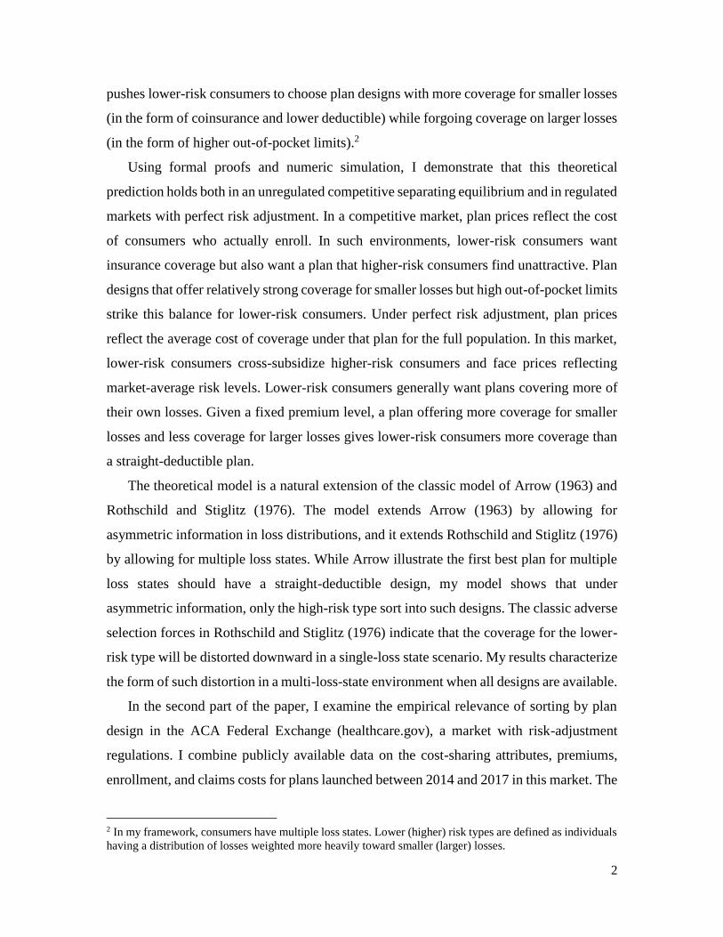
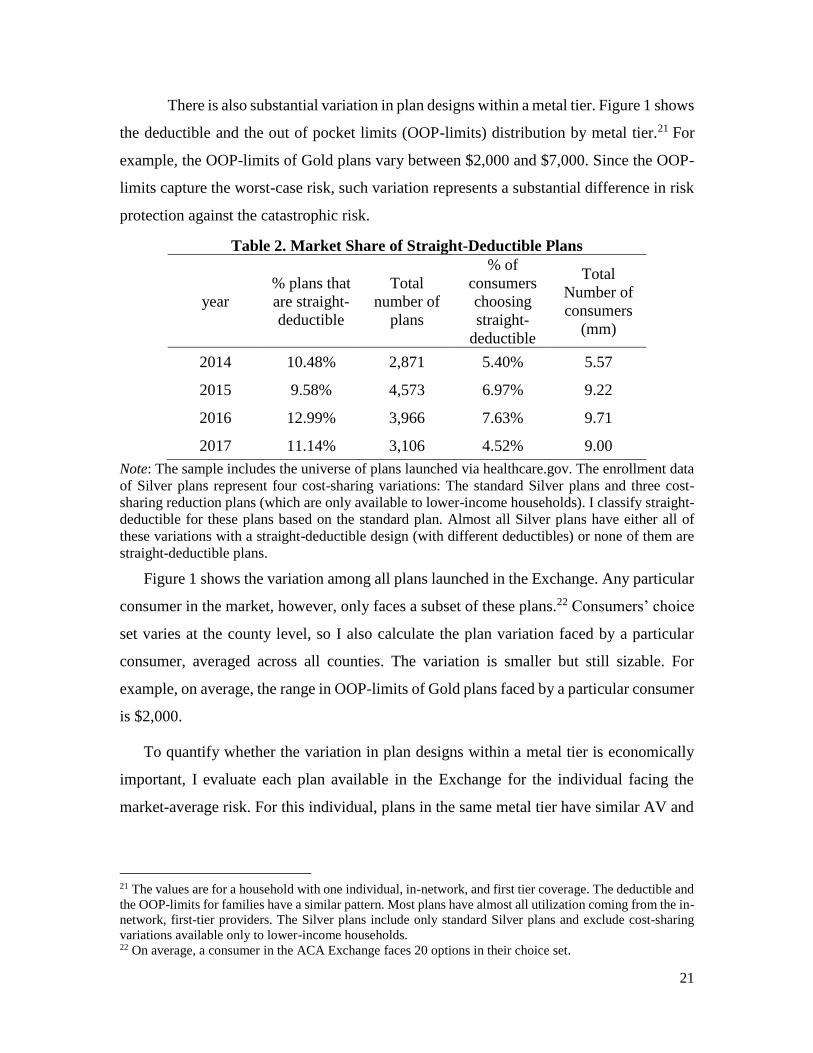
There is also substantial variation in plan designs within a metal tier. Figure 1 shows

the deductible and the out of pocket limits (OOP-limits) distribution by metal tier.21 For

example, the OOP-limits of Gold plans vary between $2,000 and $7,000. Since the OOP-

limits capture the worst-case risk, such variation represents a substantial difference in risk

protection against the catastrophic risk.

Table 2. Market Share of Straight-Deductible Plans

year

% plans that

are straight-

deductible

Total

number of

plans

% of

consumers

choosing

straight-

deductible

Total

Number of

consumers

(mm)

2014 10.48% 2,871 5.40% 5.57

2015 9.58% 4,573 6.97% 9.22

2016 12.99% 3,966 7.63% 9.71

2017 11.14% 3,106 4.52% 9.00

Note: The sample includes the universe of plans launched via healthcare.gov. The enrollment data

of Silver plans represent four cost-sharing variations: The standard Silver plans and three cost-

sharing reduction plans (which are only available to lower-income households). I classify straight-

deductible for these plans based on the standard plan. Almost all Silver plans have either all of

these variations with a straight-deductible design (with different deductibles) or none of them are

straight-deductible plans.

Figure 1 shows the variation among all plans launched in the Exchange. Any particular

consumer in the market, however, only faces a subset of these plans.22 Consumers’ choice

set varies at the county level, so I also calculate the plan variation faced by a particular

consumer, averaged across all counties. The variation is smaller but still sizable. For

example, on average, the range in OOP-limits of Gold plans faced by a particular consumer

is $2,000.

To quantify whether the variation in plan designs within a metal tier is economically

important, I evaluate each plan available in the Exchange for the individual facing the

market-average risk. For this individual, plans in the same metal tier have similar AV and

21 The values are for a household with one individual, in-network, and first tier coverage. The deductible and

the OOP-limits for families have a similar pattern. Most plans have almost all utilization coming from the in-

network, first-tier providers. The Silver plans include only standard Silver plans and exclude cost-sharing

variations available only to lower-income households. 22 On average, a consumer in the ACA Exchange faces 20 options in their choice set.

22

thus provide similar expected coverage. To capture the variation in plan design, I calculate

the risk premium 𝑅, defined by the following formula:

𝐸[𝑢(𝑤 − 𝑎)] = 𝑢 (𝑤 − 𝐸(𝑎) − 𝑅),

where 𝑤 represents the wealth level, 𝑎 represents the stochastic out-of-pocket spending

and 𝐸(𝑎) represents its expected value, and 𝑢(∙) is the utility function. The risk premium

for a plan is defined relative to a full-insurance benchmark. It represents the sure amount a

person would need to receive to be indifferent between enrolling in that plan versus a full-

insurance plan, when both plans are priced at their fair actuarial value. The risk premium

is zero for a risk-neutral enrollee and is positive for risk-averse individuals. It increases

when the level of uninsured risk increases.

Figure 1. Distribution of the Deductible and the OOP-Limits by Metal Tier

Deductible

OOP-Limits

Note: Data from 2017 CMS Health Insurance Exchange Public Use Files. The sample includes all

Exchange qualified health plans offered to individuals through the Health Insurance Exchange. For

Silver tier, the sample excludes the cost-sharing reduction plans.

To calculate the risk premium, I follow the literature in measuring the financial value

of health insurance (for example, Handel 2013). I use the CARA utility model, so the

wealth level is irrelevant. I set the risk-averse benchmark coefficient at 0.0004, which is

23

the mean and median of the risk aversion estimated by Handel (2013) from health insurance

plan choices after accounting for inertia. I also obtain the market-average risk in the ACA

Exchange from the 2017 Actuarial Value Calculator.23 I also calculate, for each plan, the

expected value of the covered losses for individuals facing a loss distribution as in the 2017

Actuarial Value Calculator.

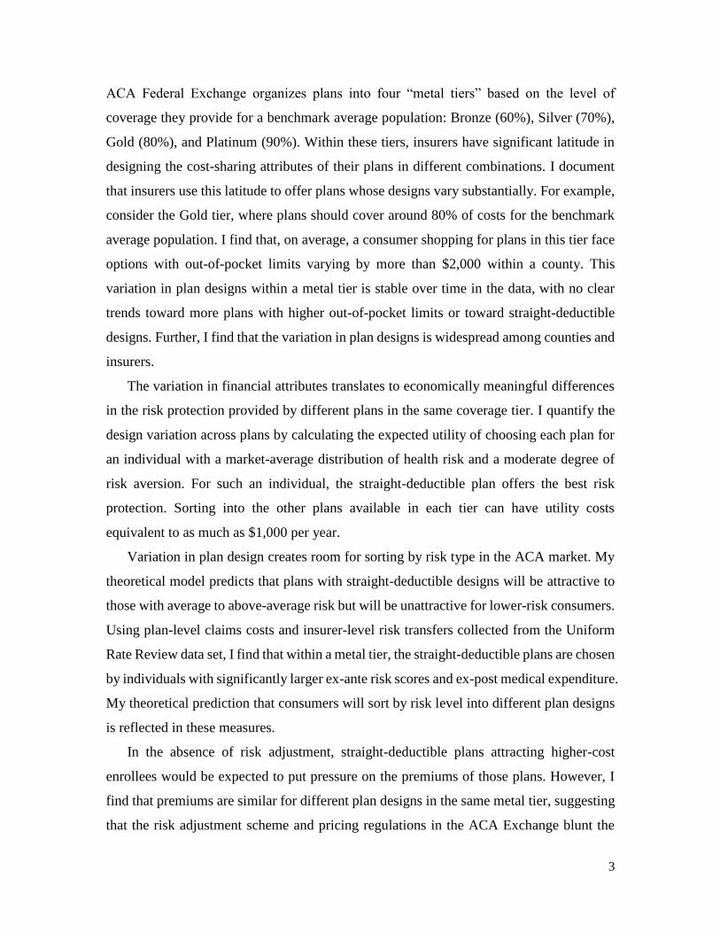
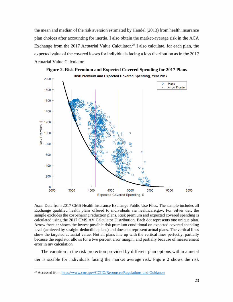
Figure 2. Risk Premium and Expected Covered Spending for 2017 Plans

Note: Data from 2017 CMS Health Insurance Exchange Public Use Files. The sample includes all

Exchange qualified health plans offered to individuals via healthcare.gov. For Silver tier, the

sample excludes the cost-sharing reduction plans. Risk premium and expected covered spending is

calculated using the 2017 CMS AV Calculator Distribution. Each dot represents one unique plan.

Arrow frontier shows the lowest possible risk premium conditional on expected covered spending

level (achieved by straight-deductible plans) and does not represent actual plans. The vertical lines

show the targeted actuarial value. Not all plans line up with the vertical lines perfectly, partially

because the regulator allows for a two percent error margin, and partially because of measurement

error in my calculation.

The variation in the risk protection provided by different plan options within a metal

tier is sizable for individuals facing the market average risk. Figure 2 shows the risk

23 Accessed from https://www.cms.gov/CCIIO/Resources/Regulations-and-Guidance/

24

premium and the expected covered spending for all plans in the four metal tiers for 2017.

The expected covered spending is a scaled function of AV, and the target metal tier is

represented by the vertical lines. A substantial difference in risk premium exists for a range

of AV levels. For example, among plans in the Silver tier, which have an AV around 70%,

the smallest risk premium relative to full insurance is around $500 and is achieved by the

straight-deductible plan (black line in Figure 2). In contrast, the largest risk premium for

Silver plans is nearly $1,000 larger, originating from plans that have lower deductibles and

OOP-limits closer to the maximum allowed by the regulation.

In Appendix D, I show that the variation is stable over time, and not correlated to

aggregate demand differences and insurer characteristics. I examine whether the risk

premium variation is different 1) among different network types, 2) in larger, more

competitive markets, and 3) whether there is a difference in plan design offering by for-

profit insurers versus non-profit insurers, or by insurer size (measured by total premium

and enrollment). None of these factors appear to correlate with plan design variations.

Rather, the variation in plan design seems to be prevalent in many different markets and

among different insurers.

3.4 Evidence of Sorting by Health into Different Plan Designs

The existence of the plan design variation creates room for selection. The theoretical

analyses in Section 2 suggest that the straight-deductible designs are more attractive to the

higher-risk types. In this section, I examine whether this theory is consistent with the

empirical pattern in the context of the ACA Federal Exchange.

3.4.1 Data

In the theoretical framework in Section 2, risk types are defined based on the

probability of incurring a range of losses. Thus, an ideal test for the sorting pattern requires

observing the full distribution of individuals enrolled in different plans. Unfortunately, I

don’t have that information for all plans available in the ACA Exchange. Instead, I focus

on testing the first moment of the loss distribution. That is, I examine whether straight-

deductible plans attract individuals with higher (ex-ante) mean expenditure. According to

Corollary 1 in Section 2, individuals sorting into straight-deductible plans have higher

mean expenditure under perfect risk adjustment.

25

The data I use is the Uniform Rate Review data. The first part of the data contains

premium and claims cost information at the plan level. The rate review regulation requires

insurers operating on the Exchange to submit justification for any plan experiencing a

premium increase of more than 10%.24 The justification includes detailed information on

average premium and the average total medical expenditure during the last period. The

total medical expenditure is the ex-post expenditure incurred by enrollees in a plan,

including the insurer's liability, consumers’ cost-sharing, and any government payment

toward medical treatment for the low-income households. I link about half of the plans in

my sample with this information between 2014 and 2017, inclusive (the claims sample

henceforth).

The second part of the data has premium and claims information at the insurer level.

Unlike the plan-level information, all insurers are required to report insurer-level data,

giving a better representation of the overall sample. I can link 75% of the insurers with

plan-level information to the Uniform Rate Review data (baseline insurer sample). For the

rest of the insurers, I match almost all of them in the Medical Loss Ratio filings, another

insurer-level dataset reporting premium and insurer loss ratio information, but only for a

limited number of variables of interest. Results using the Medical Loss Ratio data are

similar and are presented in Appendix E.

3.4.2 Methodology

I measure the extent to which plans with a non-straight deductible design attract

healthier enrollees than straight deductible designs in three ways. First, I examine the ex-

post reported total medical expenditure between straight-deductible plans and the other

designs within an insurer. There is a concern that the claims sample is biased because these

plans are relatively “underpriced” and experience a higher premium increase. As a result,

the sorting pattern may be confounded by other factors. To account for that concern, I

leverage the fact that insurers are subject to the single risk pool requirement when setting

a premium. This means if one particular plan experiences unexpected medical expenditure

increases, the insurers are required to spread out these costs among the premiums of all

plans offered, making all plans subject to reporting. In the claims sample, the majority

24 In my dataset, insurers are a unique combination of insurer-state. I use “insurer” henceforth to represent

insurer-state.

26

(75%) of insurers report either all or none of their plans in this sample. As such, while the

selection of insurers who have claims information at plan-level is a biased sub-sample,

within each insurer, there is a more representative set of the plans they offer. In my plan-

level analysis, I include insurer-year fixed effects so that the differences in claims costs

between different plan designs are identified off of within-insurer variation.

Second, I examine the average medical expenditure at the insurer level as a function of

the enrollment share in straight-deductible plans. Since all insurers are required to report

the insurer-level information, there is less concern that the sample is biased when using the

insurer-level sample.

Third, I examine the level of ex-ante risk adjustment transfers given to insurers as a

function of the share of their plans that are straight deductible. The risk transfers will

disentangle the impacts of moral hazard from adverse selection. This is because risk

adjustment payments are calculated based on the average risk score of an insurer’s

enrollees, which is a function of demographic information and pre-existing risk factors

calculated from prior claims information. The risk transfers thus reflect an ex-ante medical

expenditure risk other than moral hazard responses.25 This identification strategy is similar

to Polyakova (2016).

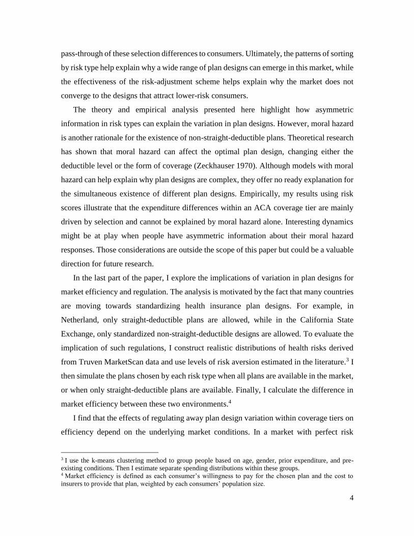
3.4.3 Selection Pattern in the Federal Exchange

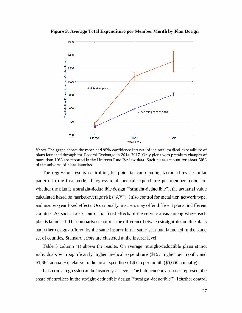
A comparison in unconditional means of the total medical expenditure illustrates that

there is a strong correlation between average medical spending and plan designs, consistent

with the theoretical predictions on sorting. Figure 3 shows the average monthly total

medical expenditure (including insurer payment and consumer cost-sharing) for straight-

deductible plans and the other designs across the metal tiers for plans in the claims sample.

Holding fixed the metal tier, the straight-deductible plans have higher medical expenditure

than the other plans. The difference is more than $400 per month for Silver and Gold

plans.26

25 Plan-level risk transfers are also estimated by insurers for a subset of plans. However, not all insurers report

their methodology of allocating the insurer-level risk transfers to the plan level. For those who do report,

some insurers use plan premiums to allocate the transfers, making the measure inappropriate to capture

selection within a metal tier. (As shown below in Table 3, different designs have similar premiums within a

metal tier.) As such, I do not include plan-level risk transfers in the analysis. 26 The difference in the Bronze tier is smaller because the OOP-limit regulation limited the room for design

difference. There are few Platinum plans in the market, so they are not shown in the graph.

27

Figure 3. Average Total Expenditure per Member Month by Plan Design

Notes: The graph shows the mean and 95% confidence interval of the total medical expenditure of

plans launched through the Federal Exchange in 2014-2017. Only plans with premium changes of

more than 10% are reported in the Uniform Rate Review data. Such plans account for about 50%

of the universe of plans launched.

The regression results controlling for potential confounding factors show a similar

pattern. In the first model, I regress total medical expenditure per member month on

whether the plan is a straight-deductible design (“straight-deductible”), the actuarial value

calculated based on market-average risk (“AV”). I also control for metal tier, network type,

and insurer-year fixed effects. Occasionally, insurers may offer different plans in different

counties. As such, I also control for fixed effects of the service areas among where each

plan is launched. The comparison captures the difference between straight-deductible plans

and other designs offered by the same insurer in the same year and launched in the same

set of counties. Standard errors are clustered at the insurer level.

Table 3 column (1) shows the results. On average, straight-deductible plans attract

individuals with significantly higher medical expenditure ($157 higher per month, and

$1,884 annually), relative to the mean spending of $555 per month ($6,660 annually).

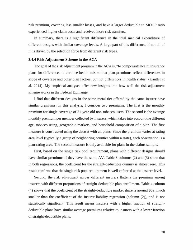
I also run a regression at the insurer-year level. The independent variables represent the

share of enrollees in the straight-deductible design (“straight-deductible”). I further control

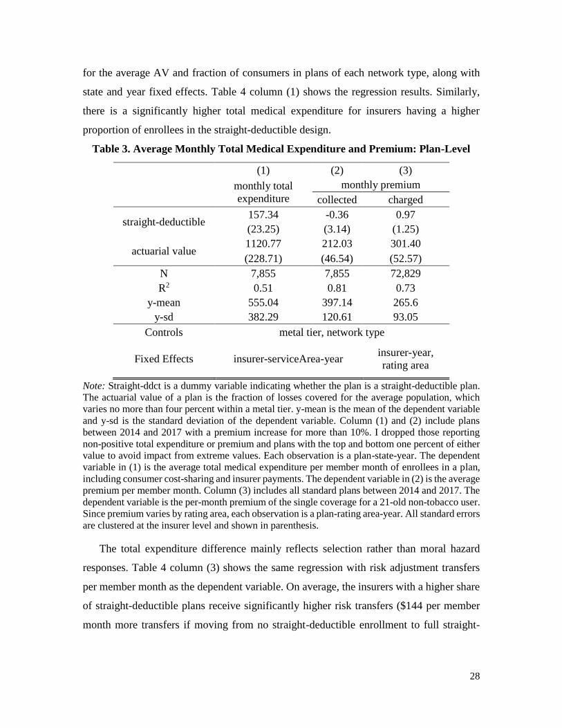
28

for the average AV and fraction of consumers in plans of each network type, along with

state and year fixed effects. Table 4 column (1) shows the regression results. Similarly,

there is a significantly higher total medical expenditure for insurers having a higher

proportion of enrollees in the straight-deductible design.

Table 3. Average Monthly Total Medical Expenditure and Premium: Plan-Level

(1) (2) (3) monthly total

expenditure

monthly premium

collected charged

straight-deductible 157.34 -0.36 0.97

(23.25) (3.14) (1.25)

actuarial value 1120.77 212.03 301.40

(228.71) (46.54) (52.57)

N 7,855 7,855 72,829

R2 0.51 0.81 0.73

y-mean 555.04 397.14 265.6

y-sd 382.29 120.61 93.05

Controls metal tier, network type

Fixed Effects insurer-serviceArea-year insurer-year,

rating area

Note: Straight-ddct is a dummy variable indicating whether the plan is a straight-deductible plan.

The actuarial value of a plan is the fraction of losses covered for the average population, which

varies no more than four percent within a metal tier. y-mean is the mean of the dependent variable

and y-sd is the standard deviation of the dependent variable. Column (1) and (2) include plans

between 2014 and 2017 with a premium increase for more than 10%. I dropped those reporting

non-positive total expenditure or premium and plans with the top and bottom one percent of either

value to avoid impact from extreme values. Each observation is a plan-state-year. The dependent

variable in (1) is the average total medical expenditure per member month of enrollees in a plan,

including consumer cost-sharing and insurer payments. The dependent variable in (2) is the average

premium per member month. Column (3) includes all standard plans between 2014 and 2017. The

dependent variable is the per-month premium of the single coverage for a 21-old non-tobacco user.

Since premium varies by rating area, each observation is a plan-rating area-year. All standard errors

are clustered at the insurer level and shown in parenthesis.

The total expenditure difference mainly reflects selection rather than moral hazard

responses. Table 4 column (3) shows the same regression with risk adjustment transfers

per member month as the dependent variable. On average, the insurers with a higher share

of straight-deductible plans receive significantly higher risk transfers ($144 per member

month more transfers if moving from no straight-deductible enrollment to full straight-

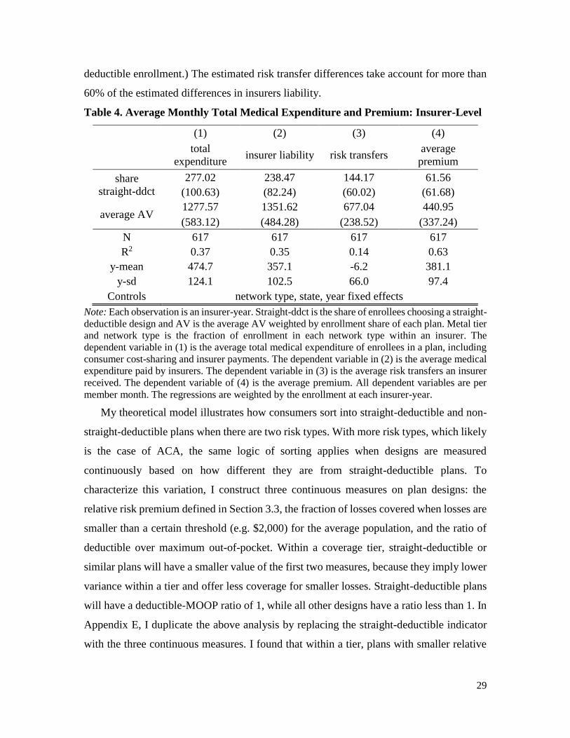
29

deductible enrollment.) The estimated risk transfer differences take account for more than

60% of the estimated differences in insurers liability.

Table 4. Average Monthly Total Medical Expenditure and Premium: Insurer-Level

(1) (2) (3) (4)

total

expenditure insurer liability risk transfers

average

premium

share

straight-ddct

277.02 238.47 144.17 61.56

(100.63) (82.24) (60.02) (61.68)

average AV 1277.57 1351.62 677.04 440.95

(583.12) (484.28) (238.52) (337.24)

N 617 617 617 617

R2 0.37 0.35 0.14 0.63

y-mean 474.7 357.1 -6.2 381.1

y-sd 124.1 102.5 66.0 97.4

Controls network type, state, year fixed effects

Note: Each observation is an insurer-year. Straight-ddct is the share of enrollees choosing a straight-

deductible design and AV is the average AV weighted by enrollment share of each plan. Metal tier

and network type is the fraction of enrollment in each network type within an insurer. The

dependent variable in (1) is the average total medical expenditure of enrollees in a plan, including

consumer cost-sharing and insurer payments. The dependent variable in (2) is the average medical

expenditure paid by insurers. The dependent variable in (3) is the average risk transfers an insurer

received. The dependent variable of (4) is the average premium. All dependent variables are per

member month. The regressions are weighted by the enrollment at each insurer-year.

My theoretical model illustrates how consumers sort into straight-deductible and non-

straight-deductible plans when there are two risk types. With more risk types, which likely

is the case of ACA, the same logic of sorting applies when designs are measured

continuously based on how different they are from straight-deductible plans. To

characterize this variation, I construct three continuous measures on plan designs: the

relative risk premium defined in Section 3.3, the fraction of losses covered when losses are

smaller than a certain threshold (e.g. $2,000) for the average population, and the ratio of

deductible over maximum out-of-pocket. Within a coverage tier, straight-deductible or

similar plans will have a smaller value of the first two measures, because they imply lower

variance within a tier and offer less coverage for smaller losses. Straight-deductible plans

will have a deductible-MOOP ratio of 1, while all other designs have a ratio less than 1. In

Appendix E, I duplicate the above analysis by replacing the straight-deductible indicator

with the three continuous measures. I found that within a tier, plans with smaller relative

30

risk premium, covering less smaller losses, and have a larger deductible to MOOP ratio

experienced higher claim costs and received more risk transfers.

In summary, there is a significant difference in the total medical expenditure of

different designs with similar coverage levels. A large part of this difference, if not all of

it, is driven by the selection force from different risk types.

3.4.4 Risk Adjustment Scheme in the ACA

The goal of the risk adjustment program in the ACA is, “to compensate health insurance

plans for differences in enrollee health mix so that plan premiums reflect differences in

scope of coverage and other plan factors, but not differences in health status” (Kautter et

al. 2014). My empirical analyses offer new insights into how well the risk adjustment

scheme works in the Federal Exchange.

I find that different designs in the same metal tier offered by the same insurer have

similar premiums. In this analysis, I consider two premiums. The first is the monthly

premium for single coverage of 21-year-old non-tobacco users. The second is the average

monthly premium per member collected by insurers, which takes into account the different

age, tobacco-using, geographic markets, and household composition of a plan. The first

measure is constructed using the dataset with all plans. Since the premium varies at rating

area level (typically a group of neighboring counties within a state), each observation is a

plan-rating area. The second measure is only available for plans in the claims sample.

First, based on the single risk pool requirement, plans with different designs should

have similar premiums if they have the same AV. Table 3 columns (2) and (3) show that

in both regressions, the coefficient for the straight-deductible dummy is almost zero. This

result confirms that the single risk pool requirement is well enforced at the insurer level.

Second, the risk adjustment across different insurers flattens the premium among

insurers with different proportions of straight-deductible plan enrollment. Table 4 column

(4) shows that the coefficient of the straight-deductible market share is around $62, much

smaller than the coefficient of the insurer liability regression (column (2)), and is not

statistically significant. This result means insurers with a higher fraction of straight-

deductible plans have similar average premiums relative to insurers with a lower fraction

of straight-deductible plans.

31

Though for the most part risk adjustment flattens the premiums across different designs,

the risk adjustment scheme may be imperfect and undercompensate the straight-deductible

designs. In calculating the insurer’s likely payment toward a plan, the current risk

adjustment formula assumes a fixed plan design (non-straight-deductible) for each metal

tier. Given that the higher-risk types have more expense covered under straight-deductible

plans than other plans in the same metal tier, the current formula underestimates the actual

covered expenses of straight-deductible plans. This underestimation may partially explain

the fact that the coefficient of risk transfers (Table 4 column (3)) is smaller than the

coefficient of insurer liability (Table 4 column (2)).27

My analyses suggest that when determining the risk transfers across insurers, regulators

should account for the fact that straight-deductible plans cover more expenses for the

higher-risk types than other designs holding fixed a metal tier. A better formula to achieve

the stated goal is to have the risk transfers depend on both the metal tier and the plan design

consumers choose.

4. Implications for Plan Design Regulation

The existence of sorting by plan design has important implications for regulating the

overall health insurance market. There is a wide public policy debate on whether and how

to regulate plan designs. A few markets in the United States (including the California State

Health Insurance Exchange) and other OECD countries (including the Netherlands and

Switzerland) have adopted plan standardization regulations, mainly motivated by

consumer confusion. However, there is no consensus on what the design of standardized

plans: In the Netherlands, only straight-deductible plans are offered. In California,

standardized plans have a non-straight-deductible design.

In this section, I explore the issue using the conceptual framework developed in Section

2. The counterfactual regulation is that insurers can only offer straight-deductible plans. I

show that under asymmetric information, removing plan design variation may harm market

efficiency and make the market more likely to “unravel”, in the sense that more individuals

27 These differences may also reflect moral hazard. Note that besides risk adjustment, there are reinsurance

and risk corridor programs to further adjust for the claims costs difference among different designs. But the

reinsurance transfers will take in ex-post spending, thus are not considered here.

32

want to stay with their endowment than purchasing any insurance. I illustrate that the

impacts of such policies hinge on the existence of risk adjustment and consumer confusion.

I also estimate the likely benefits of such regulation in the ACA Federal Exchange.

Before delving into the details, I introduce two efficiency measures used throughout

the section. The first is overall efficiency, defined as the net value of providing the plan to

a certain individual minus the true costs to the society providing that coverage, weighted

across the population:

𝑊 = ∑𝑎𝑖(𝑣𝑖𝑗 − 𝜃𝑙𝑖𝑗), (4)

where 𝑎𝑖 is the relative weight of each type and 𝑣𝑖𝑗 is the value for individual 𝑖 choosing

plan 𝑗 calculated based on out-of-pocket spending (excluding premium). Under CARA

utility, which I assume throughout the simulation and estimation, 𝑣𝑖𝑗 is the certainty

equivalent of ∫ 𝑢(−𝑂𝑂𝑃𝑗)𝑑𝐹𝑖 relative to full insurance. It is separable from the costs of

providing insurance or premiums because of CARA utility. 𝜃𝑙𝑖𝑗 is the expected covered

spending multiplied by a loading factor (𝜃 =1.2). Note that the true costs to the society of

providing the plan, 𝜃𝑙𝑖𝑗, is the same as the premium only under an unregulated competitive

equilibrium, but not the same under perfect risk adjustment.

The second is type 𝑖’s consumer surplus for choosing a specific plan 𝑗:

𝑆𝑖𝑗 = 𝑣𝑖𝑗 − 𝑝𝑗 − 𝑡𝑎𝑥, (5)

where 𝑝𝑗 is the premium of the plan, 𝑡𝑎𝑥 is a uniform tax imposed on the whole population

if there is any difference in the overall premium collected and the claims costs plus loading

incurred. Unregulated competitive markets have a neutral budget, so 𝑡𝑎𝑥 = 0 . Under

perfect risk adjustment, the budget may not be neutral without tax. I assume the market

finances the difference through a tax or subsidy equally imposed on everyone in the market.

For both measures, I report the difference from the plans they choose under full

information for ease of interpretation. A positive number in the surplus means consumers

are better off than in the full information scenario. The efficiency measures are always non-

positive (because the full information is the first-best).

4.1 Design Regulation in a Competitive Equilibrium

The existence of design variation creates a mechanism for screening that allows lower-

risk type to get greater coverage while avoiding pooling with higher-risk type. Table 5

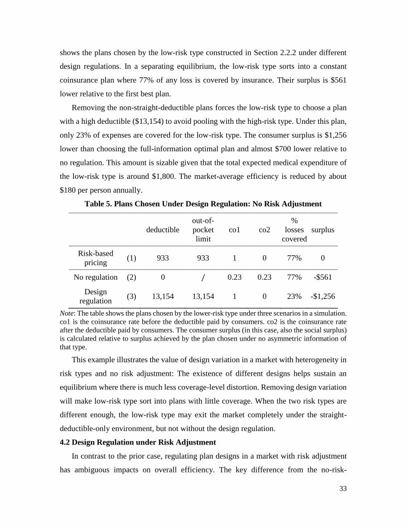
33

shows the plans chosen by the low-risk type constructed in Section 2.2.2 under different

design regulations. In a separating equilibrium, the low-risk type sorts into a constant

coinsurance plan where 77% of any loss is covered by insurance. Their surplus is $561

lower relative to the first best plan.

Removing the non-straight-deductible plans forces the low-risk type to choose a plan

with a high deductible ($13,154) to avoid pooling with the high-risk type. Under this plan,

only 23% of expenses are covered for the low-risk type. The consumer surplus is $1,256

lower than choosing the full-information optimal plan and almost $700 lower relative to

no regulation. This amount is sizable given that the total expected medical expenditure of

the low-risk type is around $1,800. The market-average efficiency is reduced by about

$180 per person annually.

Table 5. Plans Chosen Under Design Regulation: No Risk Adjustment

deductible

out-of-

pocket

limit

co1 co2

%

losses

covered

surplus

Risk-based

pricing (1) 933 933 1 0 77% 0

No regulation (2) 0 / 0.23 0.23 77% -$561

Design

regulation (3) 13,154 13,154 1 0 23% -$1,256

Note: The table shows the plans chosen by the lower-risk type under three scenarios in a simulation.

co1 is the coinsurance rate before the deductible paid by consumers. co2 is the coinsurance rate

after the deductible paid by consumers. The consumer surplus (in this case, also the social surplus)

is calculated relative to surplus achieved by the plan chosen under no asymmetric information of

that type.

This example illustrates the value of design variation in a market with heterogeneity in

risk types and no risk adjustment: The existence of different designs helps sustain an

equilibrium where there is much less coverage-level distortion. Removing design variation

will make low-risk type sort into plans with little coverage. When the two risk types are

different enough, the low-risk type may exit the market completely under the straight-

deductible-only environment, but not without the design regulation.

4.2 Design Regulation under Risk Adjustment

In contrast to the prior case, regulating plan designs in a market with risk adjustment

has ambiguous impacts on overall efficiency. The key difference from the no-risk-

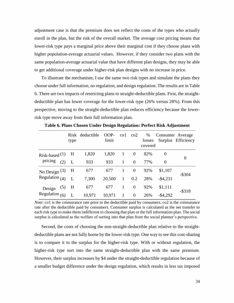
34

adjustment case is that the premium does not reflect the costs of the types who actually

enroll in the plan, but the risk of the overall market. The average cost pricing means that

lower-risk type pays a marginal price above their marginal cost if they choose plans with

higher population-average actuarial values. However, if they consider two plans with the

same population-average actuarial value that have different plan designs, they may be able

to get additional coverage under higher-risk plan designs with no increase in price.

To illustrate the mechanism, I use the same two risk types and simulate the plans they

choose under full information, no regulation, and design regulation. The results are in Table

6. There are two impacts of restricting plans to straight-deductible plans. First, the straight-

deductible plan has lower coverage for the lower-risk type (26% versus 28%). From this

perspective, moving to the straight-deductible plan reduces efficiency because the lower-

risk type move away from their full information plan.

Table 6. Plans Chosen Under Design Regulation: Perfect Risk Adjustment

Risk

type

deductible OOP-

limit

co1 co2 %

losses

covered

Consumer

Surplus

Average

Efficiency

Risk-based

pricing

(1) H 1,820 1,820 1 0 82% 0 0

(2) L 933 933 1 0 77% 0

No Design

Regulation

(3) H 677 677 1 0 92% $1,107 -$304

(4) L 7,300 20,500 1 0.2 28% -$4,231

Design

Regulation

(5) H 677 677 1 0 92% $1,111 -$318

(6) L 10,971 10,971 1 0 26% -$4,292

Note: co1 is the coinsurance rate prior to the deductible paid by consumers. co2 is the coinsurance

rate after the deductible paid by consumers. Consumer surplus is calculated as the net transfer to

each risk type to make them indifferent to choosing that plan or the full information plan. The social

surplus is calculated as the welfare of sorting into that plan from the social planner’s perspective.

Second, the costs of choosing the non-straight-deductible plan relative to the straight-

deductible plans are not fully borne by the lower-risk type. One way to see this cost-sharing

is to compare it to the surplus for the higher-risk type. With or without regulation, the

higher-risk type sort into the same straight-deductible plan with the same premium.

However, their surplus increases by $4 under the straight-deductible regulation because of

a smaller budget difference under the design regulation, which results in less tax imposed

35

overall. This difference in tax means the lower-risk type do not fully bear the costs of

choosing the non-straight-deductible plan and pass some of the costs to the higher-risk type

(in the form of higher tax). This passing on of cost is equivalent to taking on extra coverage

without paying the fair price. Removing such options removes this externality.

The two forces move in opposite directions, and the overall efficiency depends on the

relative size of the two. In this numeric example, the average efficiency is reduced by $14

under the regulation.

The regulation can also have an impact on the extensive margin. In this specific

example, the two risk types always choose some insurance over no insurance, so there is

no interaction with the extensive margin. When there is more variation in the risk types in

the market, some of the lowest risk types may choose to drop out of the market entirely

given the risk-adjusted premium. In these cases, the existence of plan design variation helps

limit market unraveling (i.e. only higher risk types buy insurance): When there are only

straight-deductible plans, the lower-risk types cannot find the plans providing enough

coverage at a reasonable price, and they are more likely to exit the market than if there are

other designs. In markets like the ACA Exchange, the premium is based on the risk of those

who participate in the market. In such markets, the exit of the lower risk types will increase

the overall premium of the market, and create a feedback loop where the fraction insured

decreases under the design regulation. In Appendix F, I provide a numeric example using

100 risk types created from the Truven MarketScan data. In the example, an additional five

percent of the population will drop out of the market when there is a design regulation

removing non-straight-deductible plans.

4.3 Consumer Confusion

Prior literature emphasizes the relevance of consumer confusion in this market

(Abaluck and Gruber 2011, Abaluck and Gruber 2019; Bhargava et al. 2017). Under

confusion, individuals may sort into a plan with a low value for them. Since in the full

information case, all types want a straight-deductible plan, limiting plans to only these

plans may help mitigate the consequence of sorting into the wrong plan.

The consequence of choosing the wrong plan is especially large for the higher-risk type.

Take the two plans chosen by the two risk types in the perfect risk adjustment case as an

example. The high-risk type loses about $3,620 in their surplus from choosing the plan

36

intended for the low-risk type. For the low-risk type, choosing the plan of the higher-risk

type is also bad for their surplus because that plan is too expensive for them. However,

from the market efficiency perspective, the low-risk type gets more coverage under the

plan chosen by the high-risk type and thus incurs positive efficiency to the society (about

$1,155). This result suggests that restricting plans to straight-deductible plans might have

sizable impacts on market efficiency with confusion and differential impacts on different

risk types.

4.4 Estimating the Effects for the ACA Federal Exchange

In this section, I calibrate the likely impacts of limiting plans to straight-deductible

designs in the 2017 ACA Federal Exchange. Specifically, I compare the market outcome

under two sets of menus: The actual 2017 plans offered in the ACA Exchange and a

hypothetical choice set replacing all options with a straight-deductible plan of the same

premium. This new choice set has the same number of options and the same premiums as

the existing one. The only difference is that all plans have a straight-deductible design.

To represent the likely risk distributions in the ACA Exchange, I create 100 risk types

from the Truven MarketScan data using the algorithm specified in Section 2.2.2. I shift the

means of these distributions so that overall, these 100 risk types have the same average

medical expenditure as in the 2017 ACA Federal Exchange. I also assume that consumers

have a constant absolute risk aversion utility function with a risk aversion coefficient of

0.0004.

To compare the market consequence under the actual choice set and this hypothetical

one, I make the following assumptions. Since I do not have information about the risk

distributions at each county, I assume that all counties have the same risk distributions. In

each county, there are a fraction of consumers who enjoy a premium subsidy or are eligible

for cost-sharing reduction plans. These plans have a much more generous design but have

the same premium as the associated standard Silver plans. I collect information on the

fraction of each subsidized type and the amount of premium subsidy from the 2017 Open

Enrollment Period County-Level Public Use File (OEP data). Finally, I assume that the

individual mandate and premium subsidy lead everyone to choose an insurance plan, so no

insurance is not in their choice set.

37

I assume that when selecting plans, individuals base their choice on a perceived utility

from choosing plan 𝑗 given by:

𝑣𝑖𝑗 = ∫ 𝑢(−𝑂𝑂𝑃𝑗 − 𝑝𝑗)𝑑𝐹𝑖 + 𝛽𝜖𝑖𝑗.

The deterministic part, ∫ 𝑢(−𝑂𝑂𝑃𝑗 − 𝑝𝑗)𝑑𝐹𝑖 , is a function of the out-of-pocket

spending and premium. It determines the welfare-relevant value of each plan 𝑗 for

individual 𝑖. For each plan, the premium 𝑝𝑗 is calculated assuming perfect risk adjustment,

such that it reflects the costs of all risk types enrolled in the plan, multiplied by a loading

factor of 1.2, and minus any premium subsidy. I assume that all risk types are equally likely

to receive a subsidy. The fraction of people with subsidy varies by county and is collected

from the OEP dataset.

The second component of the choice utility is an error component, 𝜖𝑖𝑗 that is assumed

to be i.i.d following the extreme value type one distribution. It affects the choice of each

consumer but is not relevant for welfare. The error term allows me to incorporate the

potential for consumer confusion into the simulations. Consumers in the ACA Exchange

often face a large choice set, typically around 20 options in each county, making confusion

a likely concern. In almost all counties, there are at least two designs within a metal tier.

This variation may allow different risk types to sort into plans that suit their needs, but at

the same time, it may create room for consumer confusion. The larger the scaling parameter

𝛽, in the utility function, the more randomness there will be in plan choice, which I use to

model a greater level of consumer confusion.

I calculate the impacts of limiting plans to straight-deductible plans on overall

efficiency, defined as the expected value to consumers from the chosen plan minus the

expected cost to insurer to offer the plan coverage. Since premiums and government taxes

are net transfers between consumers, they won’t affect the overall efficiency. I also

calculate the consumer surplus for people with above (below) median expected medical

expenditure (high and low risk types). The consumer surplus includes the premium and the

transfers consumers get from the government. The average of consumer surplus weighted

by each type’s population share is the overall efficiency.

Figure 4 shows the welfare difference under the straight-deductible choice set and the

current choice set. A positive surplus means consumers are better off under the straight-

deductible-only environment than facing the current ACA menu. The x-axis is the fraction

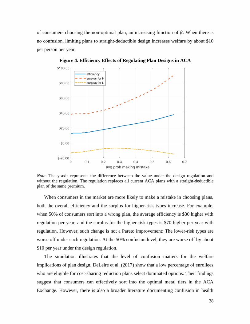
38

of consumers choosing the non-optimal plan, an increasing function of 𝛽. When there is

no confusion, limiting plans to straight-deductible design increases welfare by about $10

per person per year.

Figure 4. Efficiency Effects of Regulating Plan Designs in ACA

Note: The y-axis represents the difference between the value under the design regulation and

without the regulation. The regulation replaces all current ACA plans with a straight-deductible

plan of the same premium.

When consumers in the market are more likely to make a mistake in choosing plans,

both the overall efficiency and the surplus for higher-risk types increase. For example,

when 50% of consumers sort into a wrong plan, the average efficiency is $30 higher with

regulation per year, and the surplus for the higher-risk types is $70 higher per year with

regulation. However, such change is not a Pareto improvement: The lower-risk types are

worse off under such regulation. At the 50% confusion level, they are worse off by about

$10 per year under the design regulation.

The simulation illustrates that the level of confusion matters for the welfare

implications of plan design. DeLeire et al. (2017) show that a low percentage of enrollees

who are eligible for cost-sharing reduction plans select dominated options. Their findings

suggest that consumers can effectively sort into the optimal metal tiers in the ACA

Exchange. However, there is also a broader literature documenting confusion in health

39

insurance choices in other settings. At present, is not well understood how consumers can

best choose between plan designs with different cost-sharing designs in the ACA Exchange.

This provides an avenue for future research.

5 Conclusion

In this paper, I identify an understudied dimension of sorting in insurance markets:

Sorting by plan design. I prove that in a market with asymmetric information, lower-risk

consumers will sort into designs with less coverage for larger losses in exchange for more

coverage for smaller losses, while higher-risk consumers sort into straight-deductible plans.

The sorting pattern exists in both a separating equilibrium without price regulation and a

market with perfect risk adjustment.

This sorting pattern is empirically relevant in the US health insurance markets. I

document that in the ACA Federal Exchange, there is large variation in the cost-sharing

features of plans launched and chosen within a similar coverage level. Such variation in

cost-sharing features translates to an economically significant difference in risk protection

for consumers facing the market-average risk. I further show that within a coverage level,

the straight-deductible plans have a similar premium as the other designs, but have

significantly larger claims costs.

In sum, this paper argues for the importance of studying variation in plan design. My

framework illustrates that coverage design variation is an important dimension of sorting

under asymmetric information. This work also highlights an underappreciated perspective

in evaluating design regulations. Prior literature recognizes that simplifying insurance

contract characteristics can make it easier for consumers to compare across plans and can

promote competition and efficiency. I illustrate that in a market with asymmetric

information, plan design variation can also serve as a tool to separate different risk types

and support an equilibrium where lower-risk consumers distort less in their coverage. As a

result, removing plan design variation may make the market more likely to unravel and

harm efficiency. The overall benefits of standardizing plan design thus depend on the

relative importance of these concerns. This paper illustrates the trade-off in a market with

risk adjustment and perfect competition. More research is needed to understand the

implications of design variation when there is market power.

40

References

Abaluck, Jason, and Jonathan Gruber. “Choice Inconsistencies among the Elderly:

Evidence from Plan Choice in the Medicare Part D Program.” The American

Economic Review 101, no. 4 (June 2011): 1180–1210.

Abaluck, Jason, and Jonathan Gruber. “Less Is More: Improving Choices by Limiting

Choices in Health Insurance Markets.” Working paper (2019).

Agterberg, Joshua, Fanghao Zhong, Richard Crabb, and Marjorie Rosenberg. “A Data-

Driven Clustering Application to Identify Clusters of Individual Profiles with High

Health Expenditures.” Working paper (2019).

Aizawa, Naoki, and You Suk Kim. “Advertising and Risk Selection in Health Insurance

Markets.” American Economic Review 108, no. 3(March 2018): 828–67.

Akerlof, George. “The Market for ‘Lemons’: Quality Uncertainty and the Market

Mechanism.” The Quarterly Journal of Economics 84, no. 3 (Aug 1970) 175–188.

Arrow, Kenneth J. “Uncertainty and the Welfare Economics of Medical Care.” The

American Economic Review 53, no. 5 (1963): 941–73.

Azevedo, Eduardo M., and Daniel Gottlieb. “Perfect Competition in Markets With Adverse

Selection.” Econometrica 85, no. 1 (2017): 67–105.

Bhargava, Saurabh, George Loewenstein, and Justin Sydnor. “Choose to Lose: Health Plan

Choices from a Menu with Dominated Option.” The Quarterly Journal of Economics

132, no. 3 (August 1, 2017): 1319–72.

Brot-Goldberg, Zarek C., Amitabh Chandra, Benjamin R. Handel, and Jonathan T. Kolstad.

“What Does a Deductible Do? The Impact of Cost-Sharing on Health Care Prices,

Quantities, and Spending Dynamics.” The Quarterly Journal of Economics 132, no. 3

(August 1, 2017): 1261-1318.

Brown, Jason, Mark Duggan, Ilyana Kuziemko, and William Woolston. “How Does Risk

Selection Respond to Risk Adjustment? New Evidence from the Medicare Advantage

Program.” American Economic Review 104, no. 10 (October 2014): 3335–64.

Crocker, Keith J., and Arthur Snow. “Multidimensional Screening in Insurance Markets

with Adverse Selection.” Journal of Risk and Insurance 78, no. 2 (2011): 287–307.

DeLeire, Thomas, Andre Chappel, Kenneth Finegold, and Emily Gee. “Do Individuals

Respond to Cost-Sharing Subsidies in Their Selections of Marketplace Health

Insurance Plans?” Journal of Health Economics 56 (December 2017): 71–86.

Doherty, Neil A., and Harris Schlesinger. “Optimal Insurance in Incomplete Markets.”

Journal of Political Economy 91, no. 6 (1983): 1045–1054.

Einav, Liran, Amy Finkelstein, and Mark R. Cullen. “Estimating Welfare in Insurance

Markets Using Variation in Prices.” The Quarterly Journal of Economics 125, no. 3

(August 1, 2010): 877–921.

Einav, Liran, Amy Finkelstein, Stephen P Ryan, Paul Schrimpf, and Mark R Cullen.

“Selection on Moral Hazard in Health Insurance.” American Economic Review 103,

no. 1 (February 2013): 178–219.

Einav, Liran, Amy Finkelstein, and Pietro Tebaldi. “Market Design in Regulated Health

Insurance Markets: Risk Adjustment vs. Subsidies.” Working paper 2018.

Ericson, Keith M., and Amanda Starc. “How Product Standardization Affects Choice:

Evidence from the Massachusetts Health Insurance Exchange.” Journal of Health

Economics 50 (December 2016): 71–85.

41

Ericson, Keith M. and Justin Sydnor “Liquidity Constraints and Insurance Demand”

Working Paper 2018

Frank, Richard G, Jacob Glazer, and Thomas G McGuire. “Measuring Adverse Selection

in Managed Health Care.” Journal of Health Economics 19, no. 6 (2000): 829–54.

Finkelstein, Amy, James Poterba, and Casey Rothschild. “Redistribution by Insurance

Market Regulation: Analyzing a Ban on Gender-Based Retirement Annuities.”

Journal of Financial Economics 91, no. 1 (2009): 38–58.

Geruso, Michael, Timothy Layton, and Daniel Prinz. “Screening in Contract Design:

Evidence from the ACA Health Insurance Exchanges.” American Economic Journal:

Economic Policy 11, no. 2 (May 2019): 64–107.

Geruso, Michael, Timothy Layton, Grace McCormack, and Mark Shepard. “The Two

Margin Problem in Insurance Markets.” Working paper (2019).

Gollier, Christian, and Harris Schlesinger. “Arrow’s Theorem on the Optimality of

Deductibles: A Stochastic Dominance Approach.” Economic Theory 7, no.2 (1996):

359–63.

Handel, Benjamin R. “Adverse Selection and Inertia in Health Insurance Markets: When

Nudging Hurts.” American Economic Review 103, no. 7 (2013): 2643–82.

Handel, Ben, Igal Hendel, and Michael D. Whinston. “Equilibria in Health Exchanges:

Adverse Selection versus Reclassification Risk.” Econometrica 83, no.4 (2015):

1261–1313.

Hendren, Nathaniel. “Private Information and Insurance Rejections.” Econometrica 81, no.

5 (2013): 1713–62.

Kautter, John, Gregory Pope, Melvin Ingber, Sara Freeman, Lindsey Patterson, Michael

Cohen, and Patricia Keenan. “The HHS-HCC Risk Adjustment Model for Individual

and Small Group Markets under the Affordable Care Act.” Medicare and Medicaid

Research Review 4, no. 3 (2014): E1-E46.

Pauly, Mark V. “The Economics of Moral Hazard: Comment.” The American Economic

Review 58, no. 3 (1968): 531–537.

Polyakova, Maria. “Regulation of Insurance with Adverse Selection and Switching Costs:

Evidence from Medicare Part D.” American Economic Journal: Applied Economics 8,

no. 3 (July 2016): 165–95.

Raviv, Artur. “The Design of an Optimal Insurance Policy.” The American Economic

Review 69, no. 1 (1979): 84–96.

Rothschild, Casey. “Nonexclusivity, Linear Pricing, and Annuity Market Screening.”

Journal of Risk and Insurance 82, no. 1 (2015): 1–32.

Rothschild, Michael, and Joseph Stiglitz. “Equilibrium in Competitive Insurance Markets:

An Essay on the Economics of Imperfect Information.” The Quarterly Journal of

Economics 90, no. 4 (November 1976): 629.

Shepard, Mark. “Hospital Network Competition and Adverse Selection: Evidence from the

Massachusetts Health Insurance Exchange.” Working Paper (2016).

Spence, Michael. “Product Differentiation and Performance in Insurance Markets.”

Journal of Public Economics 10, no. 3 (December 1, 1978): 427–47.

Veiga, André, and E. Glen Weyl. “Product Design in Selection Markets.” The Quarterly

Journal of Economics 131, no. 2 (February 24, 2016): 1007-1056.

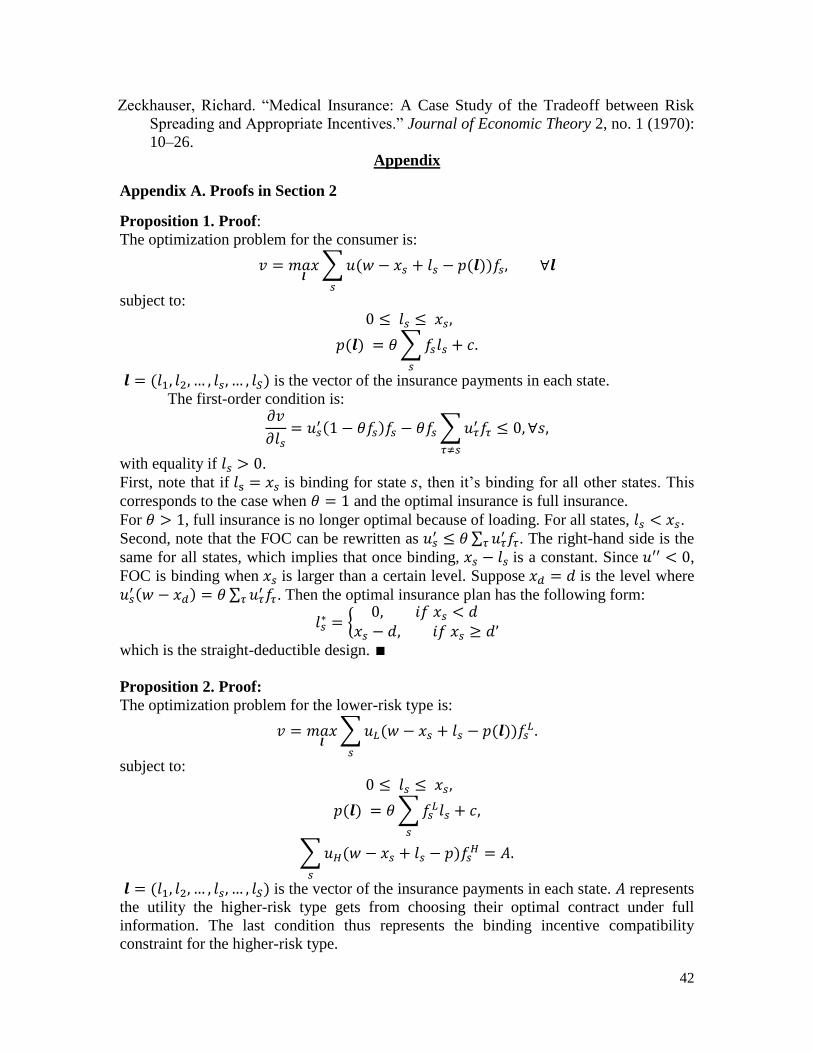
42

Zeckhauser, Richard. “Medical Insurance: A Case Study of the Tradeoff between Risk

Spreading and Appropriate Incentives.” Journal of Economic Theory 2, no. 1 (1970):

10–26.

Appendix

Appendix A. Proofs in Section 2

Proposition 1. Proof:

The optimization problem for the consumer is:

𝑣 = 𝑚𝑎𝑥𝒍

∑ 𝑢(𝑤 − 𝑥𝑠 + 𝑙𝑠

𝑠

− 𝑝(𝒍))𝑓𝑠, ∀𝒍

subject to:

0 ≤ 𝑙𝑠 ≤ 𝑥𝑠,

𝑝(𝒍) = 𝜃 ∑ 𝑓𝑠𝑙𝑠

𝑠

+ 𝑐.

𝒍 = (𝑙1, 𝑙2, … , 𝑙𝑠, … , 𝑙𝑆) is the vector of the insurance payments in each state.

The first-order condition is: 𝜕𝑣

𝜕𝑙𝑠= 𝑢𝑠

′ (1 − 𝜃𝑓𝑠)𝑓𝑠 − 𝜃𝑓𝑠 ∑ 𝑢𝜏′ 𝑓𝜏

𝜏≠𝑠

≤ 0, ∀𝑠,

with equality if 𝑙𝑠 > 0.

First, note that if 𝑙s = 𝑥𝑠 is binding for state 𝑠, then it’s binding for all other states. This

corresponds to the case when 𝜃 = 1 and the optimal insurance is full insurance.

For 𝜃 > 1, full insurance is no longer optimal because of loading. For all states, 𝑙𝑠 < 𝑥𝑠.

Second, note that the FOC can be rewritten as 𝑢𝑠′ ≤ 𝜃 ∑ 𝑢𝜏

′ 𝑓𝜏𝜏 . The right-hand side is the

same for all states, which implies that once binding, 𝑥𝑠 − 𝑙𝑠 is a constant. Since 𝑢′′ < 0,

FOC is binding when 𝑥𝑠 is larger than a certain level. Suppose 𝑥𝑑 = 𝑑 is the level where

𝑢𝑠′ (𝑤 − 𝑥𝑑) = 𝜃 ∑ 𝑢𝜏

′ 𝑓𝜏𝜏 . Then the optimal insurance plan has the following form:

𝑙𝑠∗ = {

0, 𝑖𝑓 𝑥𝑠 < 𝑑𝑥𝑠 − 𝑑, 𝑖𝑓 𝑥𝑠 ≥ 𝑑

,

which is the straight-deductible design. ∎

Proposition 2. Proof:

The optimization problem for the lower-risk type is:

𝑣 = 𝑚𝑎𝑥𝒍

∑ 𝑢𝐿(𝑤 − 𝑥𝑠 + 𝑙𝑠

𝑠

− 𝑝(𝒍))𝑓𝑠𝐿 .

subject to:

0 ≤ 𝑙𝑠 ≤ 𝑥𝑠,

𝑝(𝒍) = 𝜃 ∑ 𝑓𝑠𝐿𝑙𝑠

𝑠

+ 𝑐,

∑ 𝑢𝐻(𝑤 − 𝑥𝑠 + 𝑙𝑠

𝑠

− 𝑝)𝑓𝑠𝐻 = 𝐴.

𝒍 = (𝑙1, 𝑙2, … , 𝑙𝑠, … , 𝑙𝑆) is the vector of the insurance payments in each state. 𝐴 represents

the utility the higher-risk type gets from choosing their optimal contract under full

information. The last condition thus represents the binding incentive compatibility

constraint for the higher-risk type.

43

The Lagrange of the above optimization problem is:

ℒ(𝒍) = ∑ 𝑢𝐿(𝑤 − 𝑥𝑠 + 𝑙𝑠

𝑠

− 𝑝(𝒍))𝑓𝑠𝐿 − 𝜆(∑ 𝑢𝐻(𝑤 − 𝑥𝑠 + 𝑙𝑠

𝑠

− 𝑝(𝒍))𝑓𝑠𝐻 − 𝐴).

Let 𝑢𝐿𝑠′ denote the derivative of lower-risk type utility function with regard to

consumption in loss state 𝑠. The first-order condition is:

𝑢𝐿𝑠′ − 𝜆

𝑓𝑠𝐻

𝑓𝑠𝐿

𝑢𝐻𝑠′ ≤ 𝜃 (∑ 𝑢𝐿𝜏

′ 𝑓𝜏𝐿

𝜏

− 𝜆 ∑ 𝑢𝐻𝜏′ 𝑓𝜏

𝐻

𝜏

) ∀𝑠, (4)

with equality if 𝑙𝑠 > 0. Note that since the right-hand side is a constant, 𝑢𝐿𝑠′ − 𝜆

𝑓𝑠𝐻

𝑓𝑠𝐿 𝑢𝐻𝑠

′ is

the same across loss states with 𝑙𝑠 > 0.

Now take two loss states 𝑠 and 𝑡 such that 𝑥𝑠 ≠ 𝑥𝑡, 𝑙𝑠 > 0 and 𝑙𝑡 > 0. 𝑓𝑠

𝐻

𝑓𝑠𝐿 ≠

𝑓𝑡𝐻

𝑓𝑡𝐿 by

assumption. Suppose that a straight deductible is optimal, then 𝑙𝑠 − 𝑥𝑠 = 𝑙𝑡 − 𝑥𝑡 (equal

consumption when losses are larger than the deductible level). This then implies that

𝑢𝐿𝑠′ = 𝑢𝐿𝑡

′ and 𝑢𝐻𝑠′ = 𝑢𝐻𝑡

′ . But since 𝑓𝑠

𝐻

𝑓𝑠𝐿 ≠

𝑓𝑡𝐻

𝑓𝑡𝐿 , 𝑢𝐿𝑠

′ − 𝜆𝑓𝑠

𝐻

𝑓𝑠𝐿 𝑢𝐻𝑠

′ ≠ 𝑢𝐿𝑡′ − 𝜆

𝑓𝑡𝐻

𝑓𝑡𝐿 𝑢𝐻𝑡

′ ,

contradictory to (4). As a result, the optimal plan for the lower-risk type cannot be a

straight-deductible plan. ∎

Discussion. Proposition 2 assumes a specific form of premium: each plan’s premium

breaks even based on who enroll in the plan. More generally, I can show that without

specify the exact form of premium, straight-deductible cannot be an equilibrium for low-

risk type because there exists a Pareto improvement created by a non-straight-deductible

plan. Proposition A1 states the result.

Proposition A1. Suppose the market consists of two risk types, 𝐿 and 𝐻. Assume that for

any two loss states where 𝑥𝑠 ≠ 𝑥𝑡, we have 𝑓𝑠

𝐿

𝑓𝑠𝐻 ≠

𝑓𝑡𝐿

𝑓𝑡𝐻. For any straight-deductible plan, there

exists a non-straight deductible plan making 𝐻 indifferent and making 𝐿 strictly better off.

Proof: Fix a straight deductible plan with deductible 𝑑. Take two loss states, 𝑠 and 𝑡 such

that 𝑓𝑠

𝐻

𝑓𝑡𝐻 <

𝑓𝑠𝐿

𝑓𝑠𝐿 and 𝑥𝑠 > 𝑑, 𝑥𝑡 > 𝑑. This implies the consumption in 𝑠 and 𝑡 is the same, i.e.

𝑥𝑠 − 𝑙𝑠 = 𝑥𝑡 − 𝑙𝑡 ≡ 𝑐. Consider a marginal coverage increase in 𝑠 along the indifference curve of 𝐻:

𝑓𝑠𝐻𝑢𝐻(𝑐 + 𝛿) + 𝑓𝑡

𝐻𝑢𝐻(𝑐 − 휀) = 𝑓𝑠𝐻𝑢𝐻(𝑐) + 𝑓𝑡

𝐻𝑢𝐻(𝑐). (A1)

Equation (A1) implies that /𝑑휀 = −𝑓𝐻𝑠/𝑓𝐻

𝑡 .

Now consider a marginal coverage change in 𝑠 along the indifference curve for 𝐿:

𝑓𝑠𝐿𝑢𝐿(𝑐 + 𝛿) + 𝑓𝑡

𝐿𝑢𝐿(𝑐 − 휀) = 𝑓𝑠𝐿𝑢𝐿(𝑐) + 𝑓𝑡

𝐿𝑢𝐿(𝑐).

(A2)

Equation (A2) implies that to make 𝐿 indifferent, the relation between 𝛿 and 휀 has to be

such that /𝑑휀 = −𝑓𝐿𝑠/𝑓𝐿

𝑡 .

Given that 𝑓𝑠

𝐻

𝑓𝑡𝐻 <

𝑓𝑠𝐿

𝑓𝑠𝐿, the lower risk type is better off under the coverage increase in 𝑠 along

the indifference curve of 𝐻, while 𝐻 is indifferent. This marginal change in coverage

44

implies a non-straight-deductible coverage, because it implies differential consumption

after hitting the deductible. ∎

A direct implication for Proposition 2 is that if the ratio of the probabilities of the two

types (𝑓𝑠𝐿/𝑓𝑠

𝐻) is different across loss states, then straight-deductible plan cannot be an

equilibrium plan for 𝐿 . Otherwise, insurers could offer an incentive compatible non-

straight-deductible plan which only attracts 𝐿 and make them strictly better off. This breaks

the equilibrium where both types choose straight-deductible plans.

Proposition 3 Proof:

Take any loss state 𝑠, and assume that the 𝑓𝑠

𝐿

𝑓𝑠𝐻 = 𝛼. The first-order condition of the

coverage in state 𝑠 for the higher-risk type is:

𝑢𝑠𝐻′ ≤

𝜃(𝛼 + 1)

2∑ 𝑢𝜏𝐻

′ 𝑓𝜏𝐻

𝜏

, ∀𝑙𝑠,

with equality if 𝑙𝑠 > 0. Similarly, the first-order conditions for the lower-risk type are:

𝑢𝑠𝐿′ ≤

2𝜃

(𝛼 + 1)∑ 𝑢𝜏𝐿

′ 𝑓𝜏𝐿

𝜏

, ∀𝑙𝑠,

with equality if 𝑙𝑠 > 0.

For any two loss states 𝑥𝑡 > 𝑥𝑧, we know that 𝑓𝑡

𝐿

𝑓𝑡𝐻 <

𝑓𝑧𝐿

𝑓𝑧𝐻. This means whenever 𝑙𝑡 > 0

and 𝑙𝑧 > 0, 𝑢𝑡𝐻′ < 𝑢𝑧𝐻

′ and 𝑢𝑡𝐿′ > 𝑢𝑧𝐿

′ . Since 𝑢𝐻′′ < 0 and 𝑢𝐿

′′ < 0 , 𝑙𝐻𝑡∗ − 𝑥𝑡 ≥ 𝑙𝐻𝑧

∗ − 𝑥𝑧

and 𝑙𝐿𝑡∗ − 𝑥𝑡 ≤ 𝑙𝐿𝑧

∗ − 𝑥𝑧. That is, the consumption in state 𝑡 is always no smaller than the

consumption in 𝑧 for the higher-risk type, and the consumption in state 𝑧 is always no

smaller than the consumption in 𝑡 for the lower-risk type.

Note that among the plans with non-increasing consumption, the implied consumption in

𝑡 cannot be larger than the implied consumption in 𝑧. This means the higher-risk type will

either have zero indemnity at small loss states or a constant consumption 𝑐∗ once the

indemnity is positive. Higher-risk type would want to have larger consumption in state 𝑡

than in 𝑧, but are not able to because of the non-increasing consumption constraint.28 This

means the higher-risk type will desire a straight-deductible plan. The lower-risk type is not

constrained and will desire a plan with larger consumption for smaller losses (𝑥𝑠) than in

larger losses (𝑥𝑡), a non-straight-deductible design. ∎

Corollary 1. Suppose the market consists of two risk types, 𝐿 and 𝐻. Suppose for any two

loss states 𝑠 and 𝑡, where 𝑥𝑠 > 𝑥𝑡 , it is also true that 𝑓𝑠

𝐿

𝑓𝑠𝐻 <

𝑓𝑡𝐿

𝑓𝑡𝐻. Then 𝐸𝐿(𝑥) < 𝐸𝐻(𝑥).

Proof:

By definition, 𝐸𝐿(𝑥) = ∑ 𝑓𝑠𝐿𝑥𝑠s . 𝐸𝐻(𝑥) = ∑ 𝑓𝑠

𝐻𝑥𝑠s . Without loss of generality, suppose

loss states are ranked based on 𝑥 and there are in total 𝑛 loss states. In other words, 0 =𝑥1 < 𝑥2 < 𝑥3 < ⋯ < 𝑥𝑛.

28 The non-increasing consumption constraint implies that for any loss states z and t where 𝑥𝑡 > 𝑥𝑧 , the

allowed plan must imply 𝑐𝑡 ≤ 𝑐𝑧, where 𝑐𝑠 denote consumption in state 𝑠. Empirically, since most health

insurance plans accumulate spending over a year, almost all comprehensive health insurance plans satisfy

this condition.

45

Because ∑ 𝑓𝑠𝐿

s = ∑ 𝑓𝑠𝐻

s = 1 , there exists 1 ≤ 𝑘 < 𝑛 such that 𝑓1

𝐿

𝑓1𝐻 > ⋯ >

𝑓𝑘𝐿

𝑓𝑘𝐻 > 1 >

𝑓𝑘+1𝐿

𝑓𝑘+1𝐻 > ⋯ >

𝑓𝑛𝐿

𝑓𝑛𝐻 , otherwise say

𝑓1𝐿

𝑓1𝐻 > ⋯ >

𝑓𝑛𝐿

𝑓𝑛𝐻 > 1, then ∑ 𝑓𝑠

𝐿s > ∑ 𝑓𝑠

𝐻s , contradictory to

∑ 𝑓𝑠𝐿

s = ∑ 𝑓𝑠𝐻

s = 1.

𝐸𝐻(𝑥) − 𝐸𝐿(𝑥) = ∑ 𝑓𝑠𝐻𝑥𝑠

s

− ∑ 𝑓𝑠𝐿𝑥𝑠

s

= ∑(𝑓𝑠𝐻 − 𝑓𝑠

𝐿)𝑥𝑠

s

= ∑(𝑓𝑠𝐻 − 𝑓𝑠

𝐿)𝑥𝑠

s>k

+ ∑ (𝑓𝑠𝐻 − 𝑓𝑠

𝐿)𝑥𝑠

1≤𝑠≤𝑘

> 𝑥𝑘 ∑(𝑓𝑠𝐻 − 𝑓𝑠

𝐿)

𝑠>𝑘

+ 𝑥𝑘 ∑ (𝑓𝑠𝐻 − 𝑓𝑠

𝐿)

1≤𝑠≤𝑘

= 𝑥𝑘 ≥ 0.

Note that for any 𝑠 > 𝑘, 𝑓𝑠𝐻 − 𝑓𝑠

𝐿 > 0 and 𝑥𝑠 > 𝑥𝑘. Thus for any 𝑠 > 𝑘, (𝑓𝑠𝐻 − 𝑓𝑠

𝐿)𝑥𝑠 ≥(𝑓𝑠

𝐻 − 𝑓𝑠𝐿)𝑥𝑘. Similarly, for any 𝑠 ≤ 𝑘, 𝑓𝑠

𝐻 − 𝑓𝑠𝐿 ≤ 0 and 𝑥𝑠 ≤ 𝑥𝑘. Thus for any 𝑠 ≤ 𝑘,

(𝑓𝑠𝐻 − 𝑓𝑠

𝐿)𝑥𝑠 ≥ (𝑓𝑠𝐻 − 𝑓𝑠

𝐿)𝑥𝑘. ∎

Procedure calculating the separating equilibrium

To simulate the equilibrium plans chosen by the two risk types when there is no risk

adjustment, I use the equilibrium concepts developed by Azevedo and Gottlieb (2017). The

equilibrium is defined as a set of plans chosen by each risk type, and the premium schedule

for both the traded and non-traded plans satisfying the following proposition: any non-

traded plan has a premium such that some consumers are indifferent from buying or not,

and that premium is no larger than the costs of that consumer.

To calculate the plans chosen by each type, I use the following procedure:

1. Calculate the optimal plan for the higher-risk type when premium reflects their own

risk. Label this plan as 𝐻∗.

2. Find the subset of plans which makes the higher-risk type no better off if priced based

on the risk of the lower-risk type. Label these plans as in set 𝐶. Label the rest plans as

in set 𝐷.

3. Among plans in 𝐶, find the plan to maximize the utility of the lower-risk type. Label

this plan as 𝐿∗.

4. Assume (𝐻∗, 𝐿∗) is the separating equilibrium plan. Each is priced based on the risk of

the type who sorts into that plan.

5. The next step is to verify there exists a pricing scheme for all the other non-traded plans

satisfying the above proposition. This is equivalent to assigning a premium for each

plan assuming that they make at least one risk type indifferent to deviate and make the

other type no better off.

a. To do that, I first assign plans in set 𝐷 a premium to make the higher-risk type

indifferent from buying or not: 𝑝’𝐻.

b. I then assign plans in set 𝐶 a premium to make the lower-risk type indifferent from

buying or not (𝑝’𝐿). Among them, some will make the higher-risk type want to deviate.

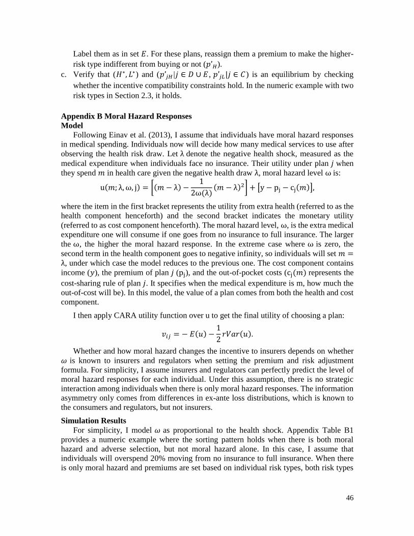
46

Label them as in set 𝐸. For these plans, reassign them a premium to make the higher-

risk type indifferent from buying or not (𝑝’𝐻).

c. Verify that (𝐻∗, 𝐿∗) and (𝑝’𝑗𝐻 |𝑗 ∈ 𝐷 ∪ 𝐸 , 𝑝’𝑗𝐿|𝑗 ∈ 𝐶) is an equilibrium by checking

whether the incentive compatibility constraints hold. In the numeric example with two

risk types in Section 2.3, it holds.

Appendix B Moral Hazard Responses

Model

Following Einav et al. (2013), I assume that individuals have moral hazard responses

in medical spending. Individuals now will decide how many medical services to use after

observing the health risk draw. Let λ denote the negative health shock, measured as the

medical expenditure when individuals face no insurance. Their utility under plan 𝑗 when

they spend 𝑚 in health care given the negative health draw λ, moral hazard level ω is:

u(𝑚; λ, ω, j) = [(𝑚 − λ) −1

2ω(λ)(𝑚 − λ)2] + [y − pj − cj(𝑚)],

where the item in the first bracket represents the utility from extra health (referred to as the

health component henceforth) and the second bracket indicates the monetary utility

(referred to as cost component henceforth). The moral hazard level, ω, is the extra medical

expenditure one will consume if one goes from no insurance to full insurance. The larger

the ω, the higher the moral hazard response. In the extreme case where ω is zero, the

second term in the health component goes to negative infinity, so individuals will set 𝑚 =λ, under which case the model reduces to the previous one. The cost component contains

income (𝑦), the premium of plan 𝑗 (pj), and the out-of-pocket costs (cj(𝑚) represents the

cost-sharing rule of plan 𝑗. It specifies when the medical expenditure is m, how much the

out-of-cost will be). In this model, the value of a plan comes from both the health and cost

component.

I then apply CARA utility function over u to get the final utility of choosing a plan:

𝑣𝑖𝑗 = − 𝐸(𝑢) −1

2𝑟𝑉𝑎𝑟(𝑢).

Whether and how moral hazard changes the incentive to insurers depends on whether

𝜔 is known to insurers and regulators when setting the premium and risk adjustment

formula. For simplicity, I assume insurers and regulators can perfectly predict the level of

moral hazard responses for each individual. Under this assumption, there is no strategic

interaction among individuals when there is only moral hazard responses. The information

asymmetry only comes from differences in ex-ante loss distributions, which is known to

the consumers and regulators, but not insurers.

Simulation Results

For simplicity, I model 𝜔 as proportional to the health shock. Appendix Table B1

provides a numeric example where the sorting pattern holds when there is both moral

hazard and adverse selection, but not moral hazard alone. In this case, I assume that

individuals will overspend 20% moving from no insurance to full insurance. When there

is only moral hazard and premiums are set based on individual risk types, both risk types

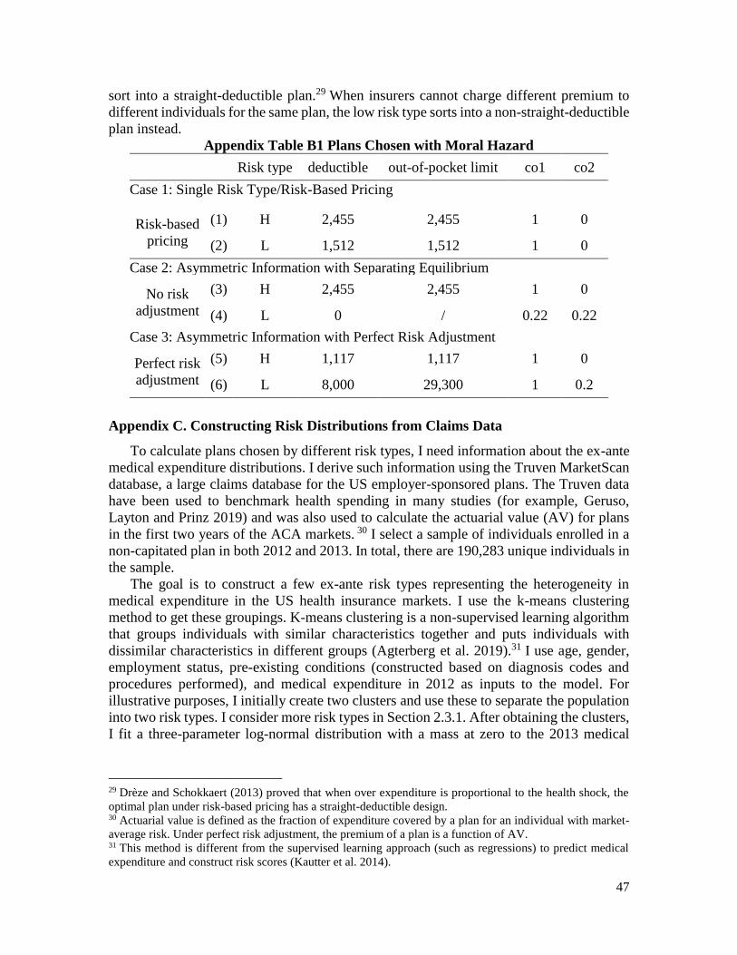
47

sort into a straight-deductible plan.29 When insurers cannot charge different premium to

different individuals for the same plan, the low risk type sorts into a non-straight-deductible

plan instead.

Appendix Table B1 Plans Chosen with Moral Hazard

Risk type deductible out-of-pocket limit co1 co2

Case 1: Single Risk Type/Risk-Based Pricing

Risk-based

pricing

(1) H 2,455 2,455 1 0

(2) L 1,512 1,512 1 0

Case 2: Asymmetric Information with Separating Equilibrium

No risk

adjustment

(3) H 2,455 2,455 1 0

(4) L 0 / 0.22 0.22

Case 3: Asymmetric Information with Perfect Risk Adjustment

Perfect risk

adjustment

(5) H 1,117 1,117 1 0

(6) L 8,000 29,300 1 0.2

Appendix C. Constructing Risk Distributions from Claims Data

To calculate plans chosen by different risk types, I need information about the ex-ante

medical expenditure distributions. I derive such information using the Truven MarketScan

database, a large claims database for the US employer-sponsored plans. The Truven data

have been used to benchmark health spending in many studies (for example, Geruso,

Layton and Prinz 2019) and was also used to calculate the actuarial value (AV) for plans

in the first two years of the ACA markets. 30 I select a sample of individuals enrolled in a

non-capitated plan in both 2012 and 2013. In total, there are 190,283 unique individuals in

the sample.

The goal is to construct a few ex-ante risk types representing the heterogeneity in

medical expenditure in the US health insurance markets. I use the k-means clustering

method to get these groupings. K-means clustering is a non-supervised learning algorithm

that groups individuals with similar characteristics together and puts individuals with

dissimilar characteristics in different groups (Agterberg et al. 2019).31 I use age, gender,

employment status, pre-existing conditions (constructed based on diagnosis codes and

procedures performed), and medical expenditure in 2012 as inputs to the model. For

illustrative purposes, I initially create two clusters and use these to separate the population

into two risk types. I consider more risk types in Section 2.3.1. After obtaining the clusters,

I fit a three-parameter log-normal distribution with a mass at zero to the 2013 medical

29 Drèze and Schokkaert (2013) proved that when over expenditure is proportional to the health shock, the

optimal plan under risk-based pricing has a straight-deductible design. 30 Actuarial value is defined as the fraction of expenditure covered by a plan for an individual with market-

average risk. Under perfect risk adjustment, the premium of a plan is a function of AV. 31 This method is different from the supervised learning approach (such as regressions) to predict medical

expenditure and construct risk scores (Kautter et al. 2014).

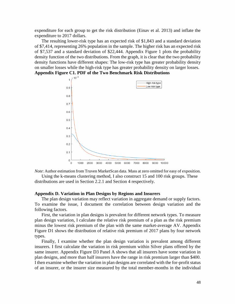
48

expenditure for each group to get the risk distribution (Einav et al. 2013) and inflate the

expenditure to 2017 dollars.

The resulting lower-risk type has an expected risk of $1,843 and a standard deviation

of $7,414, representing 26% population in the sample. The higher risk has an expected risk

of $7,537 and a standard deviation of $22,444. Appendix Figure 1 plots the probability

density function of the two distributions. From the graph, it is clear that the two probability

density functions have different shapes: The low-risk type has greater probability density

on smaller losses while the high-risk type has greater probability density on larger losses.

Appendix Figure C1. PDF of the Two Benchmark Risk Distributions

Note: Author estimation from Truven MarketScan data. Mass at zero omitted for easy of exposition.

Using the k-means clustering method, I also construct 15 and 100 risk groups. These

distributions are used in Section 2.2.1 and Section 4 respectively.

Appendix D. Variation in Plan Designs by Regions and Insurers

The plan design variation may reflect variation in aggregate demand or supply factors.

To examine the issue, I document the correlation between design variation and the

following factors.

First, the variation in plan designs is prevalent for different network types. To measure

plan design variation, I calculate the relative risk premium of a plan as the risk premium

minus the lowest risk premium of the plan with the same market-average AV. Appendix

Figure D1 shows the distribution of relative risk premium of 2017 plans by four network

types.

Finally, I examine whether the plan design variation is prevalent among different

insurers. I first calculate the variation in risk premium within Silver plans offered by the

same insurer. Appendix Figure D3 Panel A shows that all insurers have some variation in

plan designs, and more than half insurers have the range in risk premium larger than $400.

I then examine whether the variation in plan designs are correlated with the for-profit status

of an insurer, or the insurer size measured by the total member-months in the individual

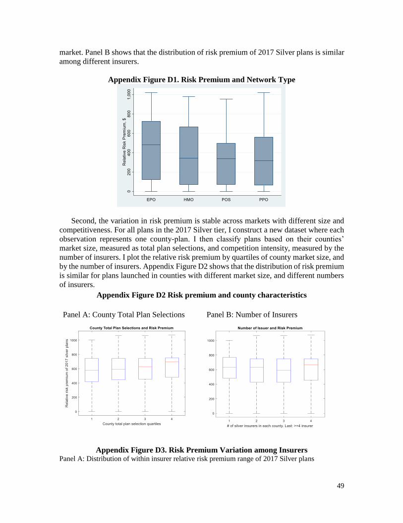
49

market. Panel B shows that the distribution of risk premium of 2017 Silver plans is similar

among different insurers.

Appendix Figure D1. Risk Premium and Network Type

Second, the variation in risk premium is stable across markets with different size and

competitiveness. For all plans in the 2017 Silver tier, I construct a new dataset where each

observation represents one county-plan. I then classify plans based on their counties’

market size, measured as total plan selections, and competition intensity, measured by the

number of insurers. I plot the relative risk premium by quartiles of county market size, and

by the number of insurers. Appendix Figure D2 shows that the distribution of risk premium

is similar for plans launched in counties with different market size, and different numbers

of insurers.

Appendix Figure D2 Risk premium and county characteristics

Panel A: County Total Plan Selections Panel B: Number of Insurers

Appendix Figure D3. Risk Premium Variation among Insurers Panel A: Distribution of within insurer relative risk premium range of 2017 Silver plans

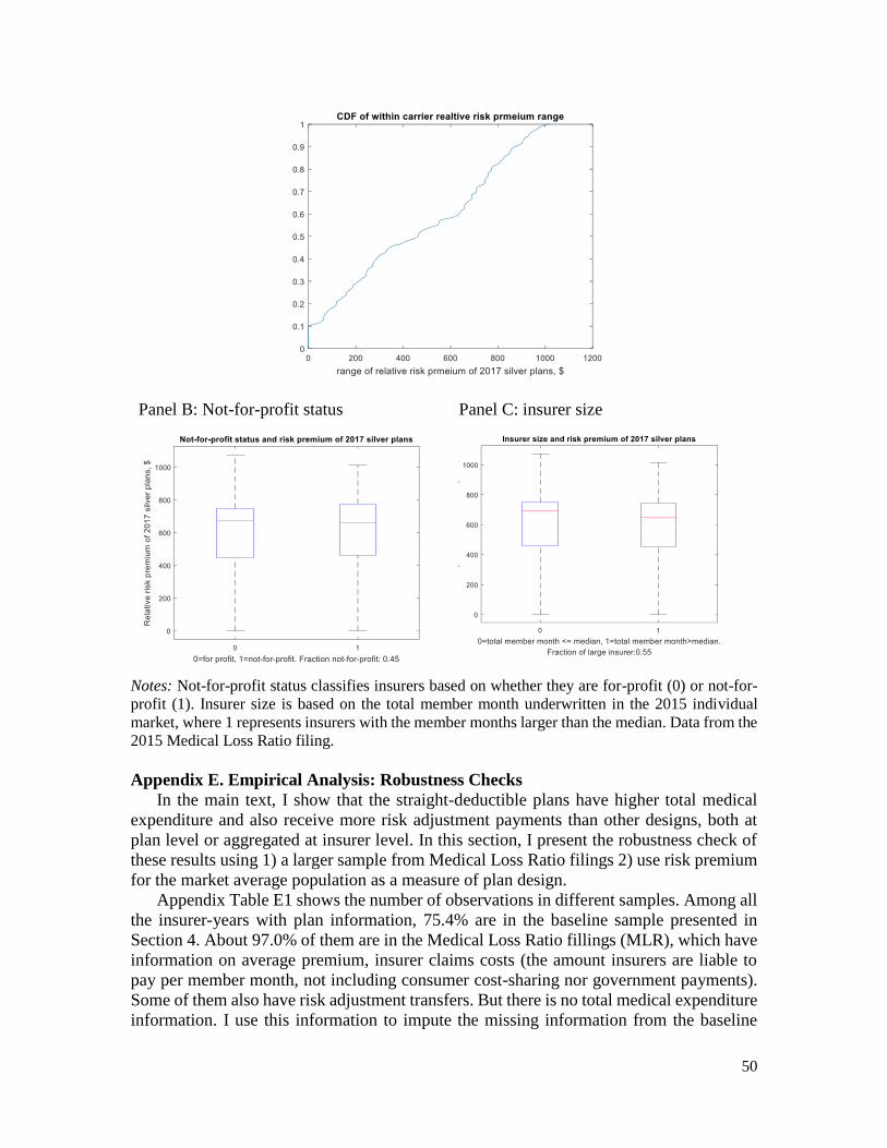
50

Panel B: Not-for-profit status Panel C: insurer size

Notes: Not-for-profit status classifies insurers based on whether they are for-profit (0) or not-for-

profit (1). Insurer size is based on the total member month underwritten in the 2015 individual

market, where 1 represents insurers with the member months larger than the median. Data from the

2015 Medical Loss Ratio filing.

Appendix E. Empirical Analysis: Robustness Checks

In the main text, I show that the straight-deductible plans have higher total medical

expenditure and also receive more risk adjustment payments than other designs, both at

plan level or aggregated at insurer level. In this section, I present the robustness check of

these results using 1) a larger sample from Medical Loss Ratio filings 2) use risk premium

for the market average population as a measure of plan design.

Appendix Table E1 shows the number of observations in different samples. Among all

the insurer-years with plan information, 75.4% are in the baseline sample presented in

Section 4. About 97.0% of them are in the Medical Loss Ratio fillings (MLR), which have

information on average premium, insurer claims costs (the amount insurers are liable to

pay per member month, not including consumer cost-sharing nor government payments).

Some of them also have risk adjustment transfers. But there is no total medical expenditure

information. I use this information to impute the missing information from the baseline

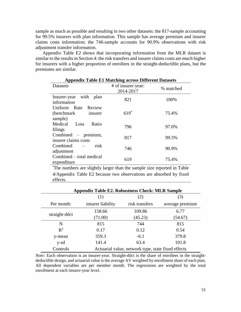
51

sample as much as possible and resulting in two other datasets: the 817-sample accounting

for 99.5% insurers with plan information. This sample has average premium and insurer

claims costs information; the 746-sample accounts for 90.9% observations with risk

adjustment transfer information.

Appendix Table E2 shows that incorporating information from the MLR dataset is

similar to the results in Section 4: the risk transfers and insurer claims costs are much higher

for insurers with a higher proportion of enrollees in the straight-deductible plans, but the

premiums are similar.

Appendix Table E1 Matching across Different Datasets

Datasets # of insurer-year:

2014-2017 % matched

Insurer-year with plan

information 821 100%

Uniform Rate Review

(benchmark insurer

sample)

619* 75.4%

Medical Loss Ratio

filings 796 97.0%

Combined – premium,

insurer claims costs 817 99.5%

Combined – risk

adjustment 746 90.9%

Combined – total medical

expenditure 619 75.4%

*The numbers are slightly larger than the sample size reported in Table

4/Appendix Table E2 because two observations are absorbed by fixed

effects.

Appendix Table E2. Robustness Check: MLR Sample

(1) (2) (3)

Per month: insurer liability risk transfers average premium

straight-ddct 158.66 109.86 6.77

(71.00) (45.23) (54.67)

N 815 744 815

R2 0.17 0.12 0.54

y-mean 359.3 -6.1 379.8

y-sd 141.4 63.4 101.8

Controls Actuarial value, network type, state fixed effects

Note: Each observation is an insurer-year. Straight-ddct is the share of enrollees in the straight-

deductible design, and actuarial value is the average AV weighted by enrollment share of each plan.

All dependent variables are per member month. The regressions are weighted by the total

enrollment at each insurer-year level.

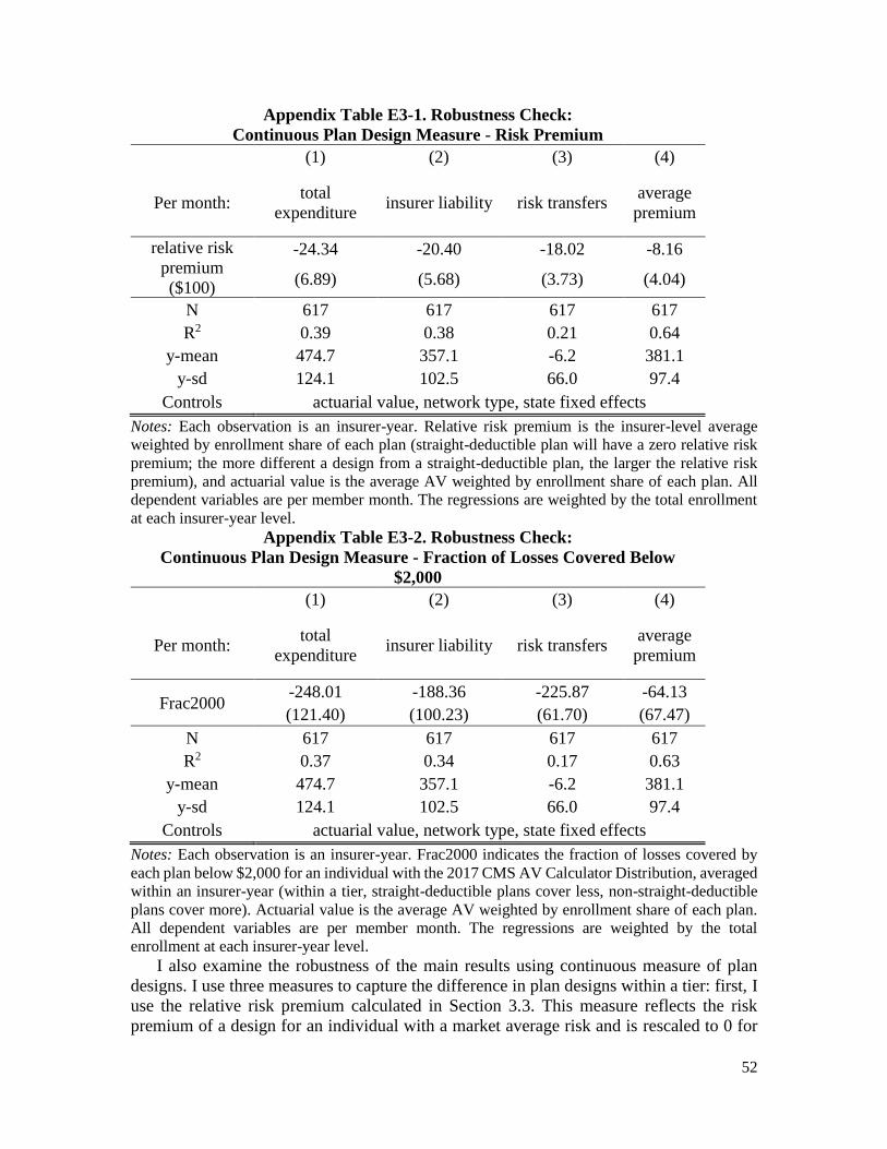
52

Appendix Table E3-1. Robustness Check:

Continuous Plan Design Measure - Risk Premium

(1) (2) (3) (4)

Per month: total

expenditure insurer liability risk transfers

average

premium

relative risk

premium

($100)

-24.34 -20.40 -18.02 -8.16

(6.89) (5.68) (3.73) (4.04)

N 617 617 617 617

R2 0.39 0.38 0.21 0.64

y-mean 474.7 357.1 -6.2 381.1

y-sd 124.1 102.5 66.0 97.4

Controls actuarial value, network type, state fixed effects

Notes: Each observation is an insurer-year. Relative risk premium is the insurer-level average

weighted by enrollment share of each plan (straight-deductible plan will have a zero relative risk

premium; the more different a design from a straight-deductible plan, the larger the relative risk

premium), and actuarial value is the average AV weighted by enrollment share of each plan. All

dependent variables are per member month. The regressions are weighted by the total enrollment

at each insurer-year level. Appendix Table E3-2. Robustness Check:

Continuous Plan Design Measure - Fraction of Losses Covered Below

$2,000

(1) (2) (3) (4)

Per month: total

expenditure insurer liability risk transfers

average

premium

Frac2000 -248.01 -188.36 -225.87 -64.13

(121.40) (100.23) (61.70) (67.47)

N 617 617 617 617

R2 0.37 0.34 0.17 0.63

y-mean 474.7 357.1 -6.2 381.1

y-sd 124.1 102.5 66.0 97.4

Controls actuarial value, network type, state fixed effects

Notes: Each observation is an insurer-year. Frac2000 indicates the fraction of losses covered by

each plan below $2,000 for an individual with the 2017 CMS AV Calculator Distribution, averaged

within an insurer-year (within a tier, straight-deductible plans cover less, non-straight-deductible

plans cover more). Actuarial value is the average AV weighted by enrollment share of each plan.

All dependent variables are per member month. The regressions are weighted by the total

enrollment at each insurer-year level.

I also examine the robustness of the main results using continuous measure of plan

designs. I use three measures to capture the difference in plan designs within a tier: first, I

use the relative risk premium calculated in Section 3.3. This measure reflects the risk

premium of a design for an individual with a market average risk and is rescaled to 0 for

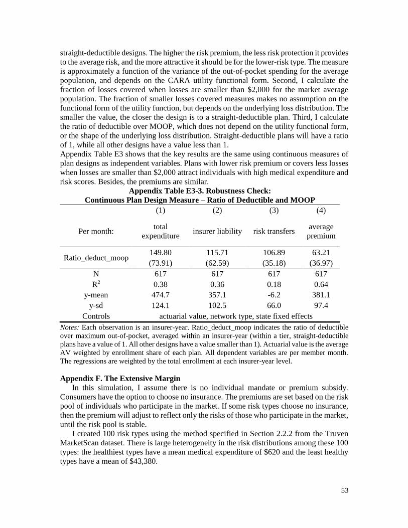
53

straight-deductible designs. The higher the risk premium, the less risk protection it provides

to the average risk, and the more attractive it should be for the lower-risk type. The measure

is approximately a function of the variance of the out-of-pocket spending for the average

population, and depends on the CARA utility functional form. Second, I calculate the

fraction of losses covered when losses are smaller than $2,000 for the market average

population. The fraction of smaller losses covered measures makes no assumption on the

functional form of the utility function, but depends on the underlying loss distribution. The

smaller the value, the closer the design is to a straight-deductible plan. Third, I calculate

the ratio of deductible over MOOP, which does not depend on the utility functional form,

or the shape of the underlying loss distribution. Straight-deductible plans will have a ratio

of 1, while all other designs have a value less than 1.

Appendix Table E3 shows that the key results are the same using continuous measures of

plan designs as independent variables. Plans with lower risk premium or covers less losses

when losses are smaller than $2,000 attract individuals with high medical expenditure and

risk scores. Besides, the premiums are similar.

Appendix Table E3-3. Robustness Check:

Continuous Plan Design Measure – Ratio of Deductible and MOOP

(1) (2) (3) (4)

Per month: total

expenditure insurer liability risk transfers

average

premium

Ratio_deduct_moop 149.80 115.71 106.89 63.21

(73.91) (62.59) (35.18) (36.97)

N 617 617 617 617

R2 0.38 0.36 0.18 0.64

y-mean 474.7 357.1 -6.2 381.1

y-sd 124.1 102.5 66.0 97.4

Controls actuarial value, network type, state fixed effects

Notes: Each observation is an insurer-year. Ratio_deduct_moop indicates the ratio of deductible

over maximum out-of-pocket, averaged within an insurer-year (within a tier, straight-deductible

plans have a value of 1. All other designs have a value smaller than 1). Actuarial value is the average

AV weighted by enrollment share of each plan. All dependent variables are per member month.

The regressions are weighted by the total enrollment at each insurer-year level.

Appendix F. The Extensive Margin

In this simulation, I assume there is no individual mandate or premium subsidy.

Consumers have the option to choose no insurance. The premiums are set based on the risk

pool of individuals who participate in the market. If some risk types choose no insurance,

then the premium will adjust to reflect only the risks of those who participate in the market,

until the risk pool is stable.

I created 100 risk types using the method specified in Section 2.2.2 from the Truven

MarketScan dataset. There is large heterogeneity in the risk distributions among these 100

types: the healthiest types have a mean medical expenditure of $620 and the least healthy

types have a mean of $43,380.

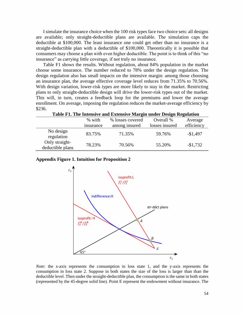
54

I simulate the insurance choice when the 100 risk types face two choice sets: all designs

are available; only straight-deductible plans are available. The simulation caps the

deductible at $100,000. The least insurance one could get other than no insurance is a

straight-deductible plan with a deductible of $100,000. Theoretically it is possible that

consumers may choose a plan with even higher deductible. The point is to think of this “no

insurance” as carrying little coverage, if not truly no insurance.

Table F1 shows the results. Without regulation, about 84% population in the market

choose some insurance. The number reduced to 78% under the design regulation. The

design regulation also has small impacts on the intensive margin: among those choosing

an insurance plan, the average effective coverage level reduces from 71.35% to 70.56%.

With design variation, lower-risk types are more likely to stay in the market. Restricting

plans to only straight-deductible design will drive the lower-risk types out of the market.

This will, in turn, creates a feedback loop for the premiums and lower the average

enrollment. On average, imposing the regulation reduces the market-average efficiency by

$236.

Table F1. The Intensive and Extensive Margin under Design Regulation

% with

insurance

% losses covered

among insured

Overall %

losses insured

Average

efficiency

No design

regulation 83.75% 71.35% 59.76% -$1,497

Only straight-

deductible plans 78.23% 70.56% 55.20% -$1,732

Appendix Figure 1. Intuition for Proposition 2

Note: the x-axis represents the consumption in loss state 1, and the y-axis represents the

consumption in loss state 2. Suppose in both states the size of the loss is larger than than the

deductible level. Then under the straight-deductible plan, the consumption is the same in both states

(represented by the 45-degree solid line). Point E represent the endowment without insurance. The

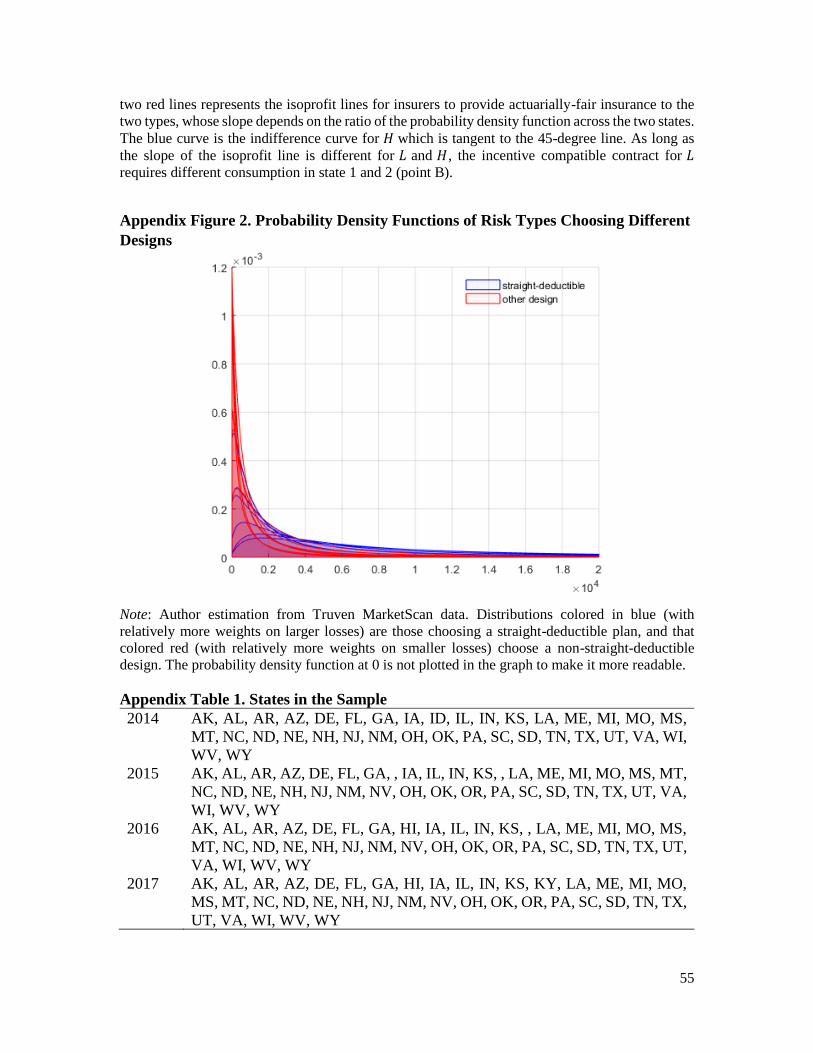
55

two red lines represents the isoprofit lines for insurers to provide actuarially-fair insurance to the

two types, whose slope depends on the ratio of the probability density function across the two states.

The blue curve is the indifference curve for 𝐻 which is tangent to the 45-degree line. As long as

the slope of the isoprofit line is different for 𝐿 and 𝐻, the incentive compatible contract for 𝐿

requires different consumption in state 1 and 2 (point B).

Appendix Figure 2. Probability Density Functions of Risk Types Choosing Different

Designs

Note: Author estimation from Truven MarketScan data. Distributions colored in blue (with

relatively more weights on larger losses) are those choosing a straight-deductible plan, and that

colored red (with relatively more weights on smaller losses) choose a non-straight-deductible

design. The probability density function at 0 is not plotted in the graph to make it more readable.

Appendix Table 1. States in the Sample

2014 AK, AL, AR, AZ, DE, FL, GA, IA, ID, IL, IN, KS, LA, ME, MI, MO, MS,

MT, NC, ND, NE, NH, NJ, NM, OH, OK, PA, SC, SD, TN, TX, UT, VA, WI,

WV, WY

2015 AK, AL, AR, AZ, DE, FL, GA, , IA, IL, IN, KS, , LA, ME, MI, MO, MS, MT,

NC, ND, NE, NH, NJ, NM, NV, OH, OK, OR, PA, SC, SD, TN, TX, UT, VA,

WI, WV, WY

2016 AK, AL, AR, AZ, DE, FL, GA, HI, IA, IL, IN, KS, , LA, ME, MI, MO, MS,

MT, NC, ND, NE, NH, NJ, NM, NV, OH, OK, OR, PA, SC, SD, TN, TX, UT,

VA, WI, WV, WY

2017 AK, AL, AR, AZ, DE, FL, GA, HI, IA, IL, IN, KS, KY, LA, ME, MI, MO,

MS, MT, NC, ND, NE, NH, NJ, NM, NV, OH, OK, OR, PA, SC, SD, TN, TX,

UT, VA, WI, WV, WY