Sorting CSE 373 Data Structures Lecture 19. 5/29/03Sorting - Lecture 192 Reading ›Sections 7.1-7.3 and 7.5 ›Section 7.6, Mergesort ›Section 7.7, Quicksort

Sorting

CSE 373

Data Structures

Lecture 19

5/29/03 Sorting - Lecture 19 2

Reading

• Reading › Sections 7.1-7.3 and 7.5

› Section 7.6, Mergesort› Section 7.7, Quicksort


Sorting

• Input› an array A of data records (Note: we have seen how to

sort when elements are in linked lists: Mergesort)

› a key value in each data record› a comparison function which imposes a

consistent ordering on the keys (e.g., integers)

• Output

› reorganize the elements of A such that• For any i and j, if i < j then A[i] A[j]


Space

• How much space does the sorting algorithm require in order to sort the collection of items?› Is copying needed? O(n) additional space› In-place sorting – no copying – O(1) additional

space› Somewhere in between for “temporary”, e.g.

O(logn) space› External memory sorting – data so large that does

not fit in memory


Time

• How fast is the algorithm?› The definition of a sorted array A says that for any

i<j, A[i] < A[j]› This means that you need to at least check on

each element at the very minimum, I.e., at least O(N)

› And you could end up checking each element against every other element, which is O(N2)

› The big question is: How close to O(N) can you get?


Stability

• Stability: Does it rearrange the order of input data records which have the same key value (duplicates)? › E.g. Phone book sorted by name. Now sort by

county – is the list still sorted by name within each county?

› Extremely important property for databases › A stable sorting algorithm is one which does not

rearrange the order of duplicate keys

n2

n·log2n

n

log2n

Faster is better!


Bubble Sort

• “Bubble” elements to to their proper place in the array by comparing elements i and i+1, and swapping if A[i] > A[i+1]› Bubble every element towards its correct position

• last position has the largest element• then bubble every element except the last one towards

its correct position• then repeat until done or until the end of the quarter,

whichever comes first ...


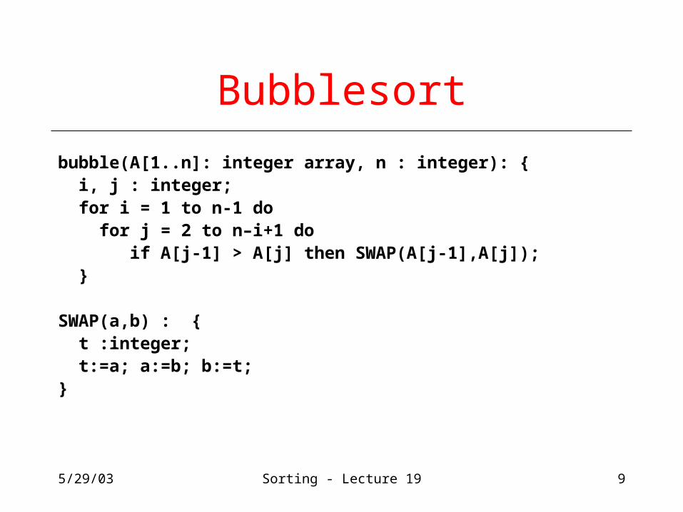
Bubblesort

bubble(A[1..n]: integer array, n : integer): { i, j : integer; for i = 1 to n-1 do for j = 2 to n–i+1 do if A[j-1] > A[j] then SWAP(A[j-1],A[j]); }

SWAP(a,b) : { t :integer; t:=a; a:=b; b:=t; }


Put the largest element in its place

1 2 3 8 7 9 10 12 23 18 15 16 17 14

2 3larger value? 8 8

7 8

swap

1 2 3 7 8 9 10 12 23 18 15 16 17 14

9 10 12 23

18 23

swap

23

15 16 17 14

18 15

swap

23 16 17 14

18 15

swap

16 23 17 14

18 15

swap

16 17 23 14

18 15

swap

16 17 14 23

1 2 3 7 8 9 10 12

1 2 3 7 8 9 10 12

1 2 3 7 8 9 10 12

1 2 3 7 8 9 10 12

1 2 3 7 8 9 10 12

9 10 12 23 18 15 16 17 141 2 3


Put 2nd largest element in its place

1 2 3 7 8 9 10 12

2 3larger value? 7 8

7 8

swap

1 2 3 7 8 9 10 12

1 2 3 7 8 9 10 12

1 2 3 7 8 9 10 12

9 10 121 2 3

18 15 16 17 14 23

15 18 16 17 14 23

9 10 12 18 18

swap

15 16 18 17 14 23swap

15 16 17 18 14 23swap

15 16 17 14 18 23

Two elements done, only n-2 more to go ...


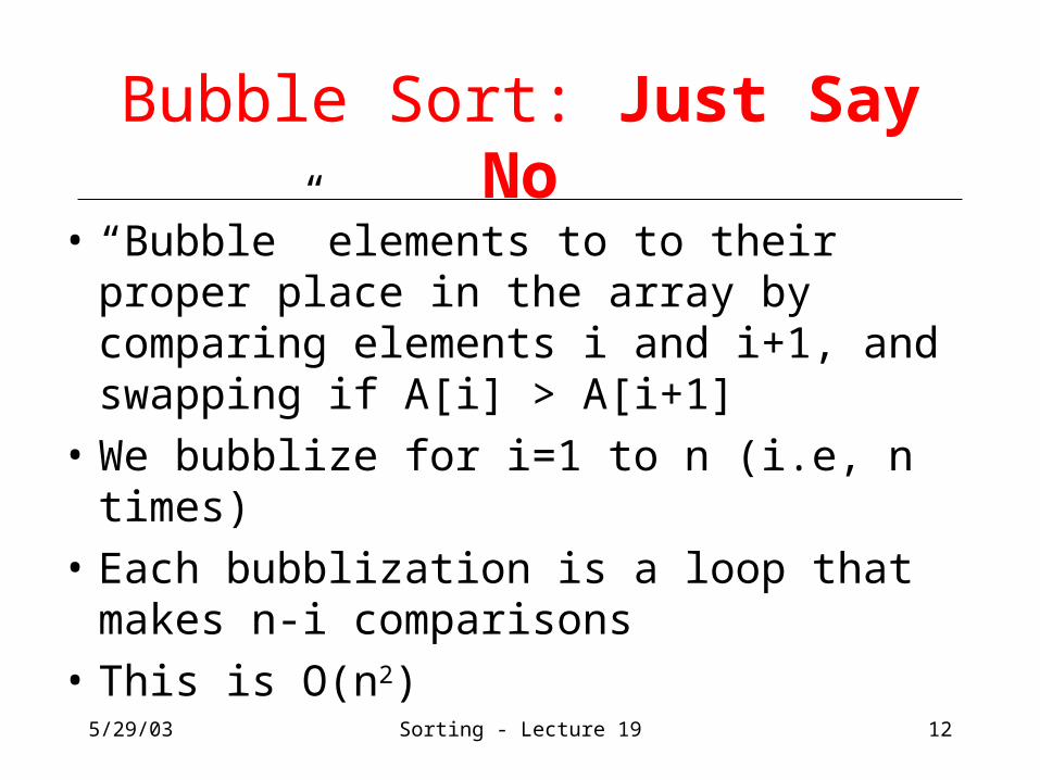
Bubble Sort: Just Say No

• “Bubble” elements to to their proper place in the array by comparing elements i and i+1, and swapping if A[i] > A[i+1]

• We bubblize for i=1 to n (i.e, n times)

• Each bubblization is a loop that makes n-i comparisons

• This is O(n2)


Insertion Sort

• What if first k elements of array are already sorted?› 4, 7, 12, 5, 19, 16

• We can shift the tail of the sorted elements list down and then insert next element into proper position and we get k+1 sorted elements› 4, 5, 7, 12, 19, 16


Insertion Sort

InsertionSort(A[1..N]: integer array, N: integer) { i, j, temp: integer ;for i = 2 to N { temp := A[i]; j := i-1; while j > 1 and A[j-1] > temp {

A[j] := A[j-1]; j := j–1;} A[j] = temp; } }

• Is Insertion sort in place? • Running time = ?


Example

1 2 3 8 7 9 10 12 23 18 15 16 17 14

1 2 3 7 8 9 10 12 23 18 15 16 17 14

18 23 15 16 17 14

18 15 23 16 17 14

15 18 23 16 17 14

15 18 16 23 17 14

1 2 3 7 8 9 10 12

1 2 3 7 8 9 10 12

1 2 3 7 8 9 10 12

1 2 3 7 8 9 10 12

15 16 18 23 17 141 2 3 7 8 9 10 12


Example

15 16 18 17 23 141 2 3 7 8 9 10 12

15 16 17 18 23 141 2 3 7 8 9 10 12

15 16 17 18 14 231 2 3 7 8 9 10 12

15 16 17 14 18 231 2 3 7 8 9 10 12

15 16 14 17 18 231 2 3 7 8 9 10 12

15 14 16 17 18 231 2 3 7 8 9 10 12

14 15 16 17 18 231 2 3 7 8 9 10 12


Insertion Sort Characteristics

• In place and Stable• Running time

› Worst case is O(N2)• reverse order input• must copy every element every time

• Good sorting algorithm for almost sorted data› Each item is close to where it belongs in

sorted order.


Heap Sort

• We use a Max-Heap• Root node = A[1]• Children of A[i] = A[2i], A[2i+1]• Keep track of current size N (number of

nodes)

N = 5

value

index

7

65

42

7 5 6 2 4

1 2 3 4 5 6 7 8


Using Binary Heaps for Sorting

• Build a max-heap• Do N DeleteMax operations

and store each Max element as it comes out of the heap

• Data comes out in largest to smallest order

• Where can we put the elements as they are removed from the heap?

BuildMax-heap

DeleteMax

7

65

42

6

45

72


1 Removal = 1 Addition• Every time we do a DeleteMax, the heap

gets smaller by one node, and we have one more node to store› Store the data at the end of the heap array› Not "in the heap" but it is in the heap array

N = 4

value

index

6 5 4 2 7

1 2 3 4 5 6 7 8

6

45

72


Repeated DeleteMax

N = 3

5 2 4 6 7

1 2 3 4 5 6 7 8

5

42

76

N = 2

4 2 5 6 7

1 2 3 4 5 6 7 8

4

52

76


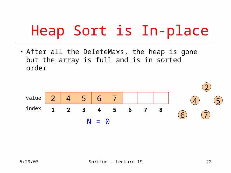
Heap Sort is In-place

• After all the DeleteMaxs, the heap is gone but the array is full and is in sorted order

N = 0

value

index

2 4 5 6 7

81 2 3 4 5 6 7

2

54

76


Heapsort: Analysis

• Running time› time to build max-heap is O(N)› time for N DeleteMax operations is N O(log N)› total time is O(N log N)

• Can also show that running time is (N log N) for some inputs, › so worst case is (N log N)› Average case running time is also O(N log N)

• Heapsort is in-place but not stable (why?)


“Divide and Conquer”

• Very important strategy in computer science:› Divide problem into smaller parts› Independently solve the parts› Combine these solutions to get overall solution

• Idea 1: Divide array into two halves, recursively sort left and right halves, then merge two halves Mergesort

• Idea 2 : Partition array into items that are “small” and items that are “large”, then recursively sort the two sets Quicksort


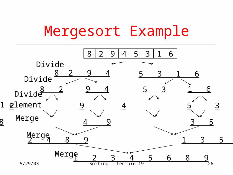
Mergesort

• Divide it in two at the midpoint

• Conquer each side in turn (by recursively sorting)

• Merge two halves together

8 2 9 4 5 3 1 6


Mergesort Example

8 2 9 4 5 3 1 6

8 2 1 69 4 5 3

8 2 9 4 5 3 1 6

2 8 4 9 3 5 1 6

2 4 8 9 1 3 5 6

1 2 3 4 5 6 8 9

Merge

Merge

Merge

Divide

Divide

Divide1 element

8 2 9 4 5 3 1 6


Auxiliary Array

• The merging requires an auxiliary array.

2 4 8 9 1 3 5 6

Auxiliary array


Auxiliary Array


2 4 8 9 1 3 5 6

1 Auxiliary array


Auxiliary Array


2 4 8 9 1 3 5 6

1 2 3 4 5 Auxiliary array


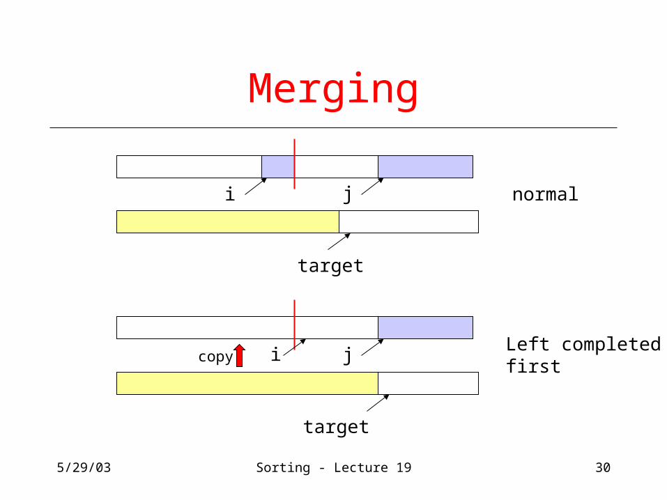
Merging

i j

target

normal

i j

target

Left completedfirst

copy


Merging

i j

target

Right completedfirst

first

second


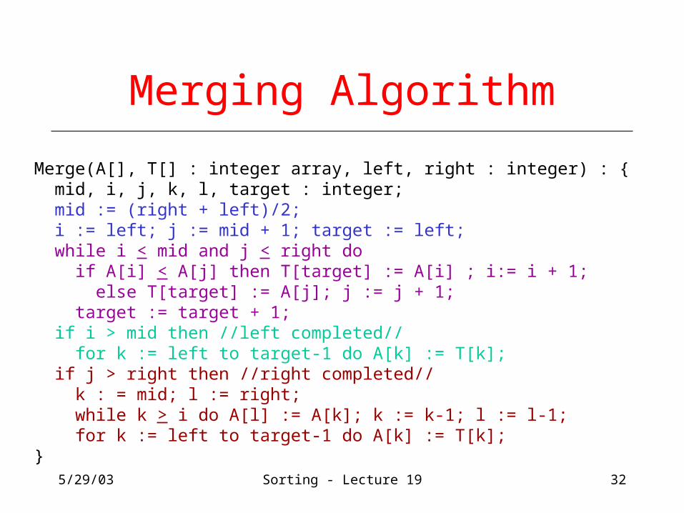
Merging Algorithm

Merge(A[], T[] : integer array, left, right : integer) : { mid, i, j, k, l, target : integer; mid := (right + left)/2; i := left; j := mid + 1; target := left; while i < mid and j < right do if A[i] < A[j] then T[target] := A[i] ; i:= i + 1; else T[target] := A[j]; j := j + 1; target := target + 1; if i > mid then //left completed// for k := left to target-1 do A[k] := T[k]; if j > right then //right completed// k : = mid; l := right; while k > i do A[l] := A[k]; k := k-1; l := l-1; for k := left to target-1 do A[k] := T[k];}


Recursive Mergesort

Mergesort(A[], T[] : integer array, left, right : integer) : { if left < right then mid := (left + right)/2; Mergesort(A,T,left,mid); Mergesort(A,T,mid+1,right); Merge(A,T,left,right);}

MainMergesort(A[1..n]: integer array, n : integer) : { T[1..n]: integer array; Mergesort[A,T,1,n];}


Iterative Mergesort

Merge by 1

Merge by 2

Merge by 4

Merge by 8


Iterative Mergesort

Merge by 1

Merge by 2

Merge by 4

Merge by 8

Merge by 16

Need of a last copy


Iterative Mergesort

IterativeMergesort(A[1..n]: integer array, n : integer) : {//precondition: n is a power of 2// i, m, parity : integer; T[1..n]: integer array; m := 2; parity := 0; while m < n do for i = 1 to n – m + 1 by m do if parity = 0 then Merge(A,T,i,i+m-1); else Merge(T,A,i,i+m-1); parity := 1 – parity; m := 2*m; if parity = 1 then for i = 1 to n do A[i] := T[i]; }

How do you handle non-powers of 2?How can the final copy be avoided?


Mergesort Analysis

• Let T(N) be the running time for an array of N elements

• Mergesort divides array in half and calls itself on the two halves. After returning, it merges both halves using a temporary array

• Each recursive call takes T(N/2) and merging takes O(N)


Mergesort Recurrence Relation

• The recurrence relation for T(N) is:› T(1) < a

• base case: 1 element array constant time

› T(N) < 2T(N/2) + bN• Sorting N elements takes

– the time to sort the left half – plus the time to sort the right half – plus an O(N) time to merge the two halves

• T(N) = O(n log n)


Properties of Mergesort

• Not in-place› Requires an auxiliary array (O(n) extra

space)

• Stable› Make sure that left is sent to target on

equal values.

• Iterative Mergesort reduces copying.


Quicksort

• Quicksort uses a divide and conquer strategy, but does not require the O(N) extra space that MergeSort does› Partition array into left and right sub-arrays

• Choose an element of the array, called pivot• the elements in left sub-array are all less than pivot• elements in right sub-array are all greater than pivot

› Recursively sort left and right sub-arrays› Concatenate left and right sub-arrays in O(1) time


“Four easy steps”

• To sort an array S1. If the number of elements in S is 0 or 1,

then return. The array is sorted.

2. Pick an element v in S. This is the pivot value.

3. Partition S-{v} into two disjoint subsets, S1 = {all values xv}, and S2 = {all values xv}.

4. Return QuickSort(S1), v, QuickSort(S2)


The steps of QuickSort

1381

92

43

65

31 57

26

750

S select pivot value

13 8192

43 6531

5726

750S1 S2

partition S

13 4331 57260

S1

81 927565

S2

QuickSort(S1) andQuickSort(S2)

13 4331 57260 65 81 9275S Voila! S is sorted[Weiss]


Details, details

• Implementing the actual partitioning

• Picking the pivot› want a value that will cause |S1| and |S2| to

be non-zero, and close to equal in size if possible

• Dealing with cases where the element equals the pivot


Quicksort Partitioning

• Need to partition the array into left and right sub-arrays› the elements in left sub-array are pivot› elements in right sub-array are pivot

• How do the elements get to the correct partition?› Choose an element from the array as the pivot

› Make one pass through the rest of the array and swap as needed to put elements in partitions


Partitioning:Choosing the pivot

• One implementation (there are others)› median3 finds pivot and sorts left, center,

right• Median3 takes the median of leftmost, middle, and

rightmost elements• An alternative is to choose the pivot randomly (need a

random number generator; “expensive”)• Another alternative is to choose the first element (but

can be very bad. Why?)

› Swap pivot with next to last element


Partitioning in-place

› Set pointers i and j to start and end of array› Increment i until you hit element A[i] > pivot› Decrement j until you hit elmt A[j] < pivot› Swap A[i] and A[j]› Repeat until i and j cross› Swap pivot (at A[N-2]) with A[i]

8 1 4 9 0 3 5 2 7 6

0 1 2 3 4 5 6 7 8 9

0 1 4 9 7 3 5 2 6 8

i j

Example

Place the largest at the rightand the smallest at the left.Swap pivot with next to last element.

Median of 0, 6, 8 is 6. Pivot is 6

Choose the pivot as the median of three


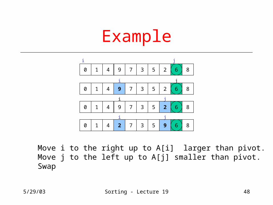
Example

0 1 4 9 7 3 5 2 6 8

0 1 4 9 7 3 5 2 6 8

i j

0 1 4 9 7 3 5 2 6 8

i j

0 1 4 2 7 3 5 9 6 8

i j

i j

Move i to the right up to A[i] larger than pivot.Move j to the left up to A[j] smaller than pivot.Swap

0 1 4 2 5 3 7 9 6 8

i j

0 1 4 2 5 3 7 9 6 86

ij

0 1 4 2 5 3 6 9 7 8

ij

S1 < pivot pivot S2 > pivot

0 1 4 2 7 3 5 9 6 8

i j

0 1 4 2 7 3 5 9 6 86

i j

0 1 4 2 5 3 7 9 6 8

i j

Example

Cross-over i > j


Recursive Quicksort

Quicksort(A[]: integer array, left,right : integer): {pivotindex : integer;if left + CUTOFF right then pivot := median3(A,left,right); pivotindex := Partition(A,left,right-1,pivot); Quicksort(A, left, pivotindex – 1); Quicksort(A, pivotindex + 1, right);else Insertionsort(A,left,right);}

Don’t use quicksort for small arrays.CUTOFF = 10 is reasonable.


Quicksort Best Case Performance

• Algorithm always chooses best pivot and splits sub-arrays in half at each recursion› T(0) = T(1) = O(1)

• constant time if 0 or 1 element

› For N > 1, 2 recursive calls plus linear time for partitioning

› T(N) = 2T(N/2) + O(N)• Same recurrence relation as Mergesort

› T(N) = O(N log N)


Quicksort Worst Case Performance

• Algorithm always chooses the worst pivot – one sub-array is empty at each recursion› T(N) a for N C› T(N) T(N-1) + bN› T(N-2) + b(N-1) + bN › T(C) + b(C+1)+ … + bN› a +b(C + (C+1) + (C+2) + … + N)› T(N) = O(N2)

• Fortunately, average case performance is O(N log N) (see text for proof)


Properties of Quicksort

• Not stable because of long distance swapping.

• No iterative version (without using a stack).• Pure quicksort not good for small arrays.• “In-place”, but uses auxiliary storage because

of recursive call (O(logn) space).• O(n log n) average case performance, but

O(n2) worst case performance.


Folklore

• “Quicksort is the best in-memory sorting algorithm.”

• Truth› Quicksort uses very few comparisons on

average.› Quicksort does have good performance in

the memory hierarchy.• Small footprint• Good locality

Documents

Sorting CSE 373 Data Structures Lecture 19. 5/29/03Sorting - Lecture 192 Reading ›Sections 7.1-7.3 and 7.5 ›Section 7.6, Mergesort ›Section 7.7, Quicksort