Sophisticated Bidders in Beauty-Contest Auctons

HAL Id: halshs-01440891https://halshs.archives-ouvertes.fr/halshs-01440891

Submitted on 19 Jan 2017

HAL is a multi-disciplinary open accessarchive for the deposit and dissemination of sci-entific research documents, whether they are pub-lished or not. The documents may come fromteaching and research institutions in France orabroad, or from public or private research centers.

L’archive ouverte pluridisciplinaire HAL, estdestinée au dépôt et à la diffusion de documentsscientifiques de niveau recherche, publiés ou non,émanant des établissements d’enseignement et derecherche français ou étrangers, des laboratoirespublics ou privés.

Sophisticated Bidders in Beauty-Contest AuctonsStefano Galavotti, Luigi Moretti, Paola Valbonesi

To cite this version:Stefano Galavotti, Luigi Moretti, Paola Valbonesi. Sophisticated Bidders in Beauty-Contest Auctons.2017. �halshs-01440891�

https://halshs.archives-ouvertes.fr/halshs-01440891

https://hal.archives-ouvertes.fr

Documents de Travail du Centre d’Economie de la Sorbonne

Sophisticated Bidders in Beauty-Contest Auctions

Stefano GALAVOTTI, Luigi MORETTI, Paola VALBONESI

2017.03

Maison des Sciences Économiques, 106-112 boulevard de L'Hôpital, 75647 Paris Cedex 13 http://centredeconomiesorbonne.univ-paris1.fr/

ISSN : 1955-611X

Sophisticated Bidders in Beauty-Contest Auctions∗

Stefano Galavotti† Luigi Moretti‡ Paola Valbonesi§

Abstract

We study bidding behavior by firms in beauty-contest auctions, i.e. auctions in whichthe winning bid is the one which gets closest to some function (average) of all submittedbids. Using a dataset on public procurement beauty-contest auctions, we show thatfirms’ observed bidding behavior departs from equilibrium and can be predicted by asophistication index, which captures the firms’ accumulated capacity of bidding close tooptimality in the past. We show that our empirical evidence is consistent with a CognitiveHierarchy model of bidders’ behavior. We also investigate whether and how firms learnto bid strategically through experience.

JEL classification: C70; D01; D44; D83; H57.Keywords: cognitive hierarchy; auctions; beauty-contest; public procurement.

∗We are indebted to Francesco Decarolis for providing us with his codes. We would like to thank for their valuablecomments: Malin Arve, Riccardo Camboni, Ottorino Chillemi, Decio Coviello, Klenio Barbosa, Gordon Klein, LucianoGreco, Marco Pagnozzi, Tim Salmon, Giancarlo Spagnolo, Alessandra Bianchi and participants at the “Workshop onEconomics of Public Procurement” (Stockholm, June 2013), International Conference on “Contracts, Procurement, andPublic-Private Arrangements” (Chaire EPPP IAE Pantheon-Sorbonne, Florence, June 2013), 54th Annual Conferenceof the Italian Economic Association (Bologna, October 2013), “Workshop on How do Governance Complexity andFinancial Constraints affect Public-Private Contracts? Theory and Empirical Evidence” (Padova, April 2014), EARIEConference (Milan, August 2014), seminar at PSE & U. Paris I Pantheon-Sorbonne (February 2015), 1st Berkeley-Paris Organizational Economics Workshop (April 2015), seminar at the Department of Economics, Leicester University(October 2015).†Corresponding author. Department of Economics and Management, University of Padova, Via

del Santo 33, 35123 Padova, Italy. Phone: +39 049 8274055. Fax: +39 049 8274221. Email: [email protected].‡Centre d’Economie de la Sorbonne, Universite Paris 1 Pantheon-Sorbonne, 106-112 Bvd de l’Hopital, 75013

Paris, France. Email: [email protected].§Department of Economics and Management, University of Padova, Via del Santo 33, 35123 Padova,

Italy; Higher School of Economics, National Research University, Moscow-Perm, Russia. Email:[email protected].

1

Documents de travail du Centre d'Economie de la Sorbonne - 2017.03

1 Introduction

The competition among firms in market economies generates winners and losers: some firmssurvive, grow up and pay dividends to their shareholders, others have poor performances orgo bankrupt and exit the market. Why does this happen? Is it because, though all firms aremaking their optimal decisions, the winners have some structural or informational advantageover the losers? Or is it simply because the losers are making the wrong decisions, or, ingame-theoretic language, they are not playing their equilibrium strategies?

Answering to this question is typically difficult, as we rarely observe all the fine detailsof the game that firms are actually playing. Moreover, even though we can replicate marketgames in controlled lab-experiment, it is questionable whether and to what extent theseinsights can be generalized to real-world situations where stakes are large.

In this paper to address the above question using field data from a peculiar procurementauction market: average bid auctions. These auctions resemble beauty-contest games in thatthe winning bid is the one which gets closest to some function (average) of all submitted bids.Average bid auctions have very precise Nash equilibrium predictions which are essentiallyunaffected by variables that are often unobservable: in equilibrium, either all or – possibly –most bids should be equal. This makes it an ideal setting to investigate possible deviationsfrom equilibrium.

Using an original dataset of procurement average bid auctions in the Italian region of Valled’Aosta, we observe that actual bids significantly depart from equilibrium, being characterizedby a systematic heterogeneity. Starting from the consideration that the peculiar rules ofthese auctions call for refined strategic thinking by bidders, as a bidder has to anticipatethe behavior of all other bidders (whereas in a first-price auction, it is sufficient to guess thedistribution of the highest competing bid), we hypothesize that the observed heterogeneitycould be the result of the interaction of firms with different abilities in performing an iteratedprocess of strategic reasoning, in the spirit of the Cognitive Hierarchy (CH, henceforth) modelby Camerer et al. (2004). Applied to our context, this model predicts that more sophisticatedfirms, being able to formulate more accurate beliefs about how others are going to bid, make“better” bids, i.e. closer to the truly optimal one. We estimate an empirical reduced formmodel which shows that, in accordance with the main prediction of the CH model, the firm’ssophistication index, measured by the accumulated capacity of bidding well in the past, isstrongly and positively correlated to the goodness of that firm’s bid, measured by the (negativeof the) distance from the truly optimal bid. This result is robust to several specifications ofthe empirical model; most importantly, it is also confirmed when we focus our analysis ona sample of auctions awarded with a new average bid format, which includes a stochasticcomponent. Interestingly, our evidence shows that a significant learning process is at work:firms become better strategic bidders as they participate in more and more auctions of thesame format; instead, sophistication acquired in one format does not significantly affectsperformance in the other.

This paper mainly contributes to two strands of literature. First, we relate to two recentpapers which fit structural econometric CH model on real data. In particular, Goldfarb andYang (2009) study the decision by Internet Service Providers whether or not to adopt the thennew 56K modem technology in 1997. Goldfarb and Xiao (2011) investigate the choice by U.S.managers of competitive local exchange carriers (CLECs) to enter local telephone marketsafter the Telecommunication Act in 1996. Both papers uncover significant heterogeneity of

2


sophistication among managers, with more sophisticated managers less likely to adopt thenew technology or to enter markets with more competitors. They also show that the levelof sophistication is higher for firms operating in larger cities, with more competitors or inmarkets with more educated populations (Goldfarb and Yang) and for more experienced,better educated managers (Goldfarb and Xiao). Both these papers assume a CH model, butdo not address whether their model fits better than an equilibrium model.1 In our paper,instead, we do not assume any structural model but show that the capacity of firms of makingbetter decisions has a systematic component which goes in a direction coherent with a CHmodel.

Second, our paper contributes to a recent empirical and experimental literature on averagebid auctions. Decarolis (2014) and Bucciol et al. (2013) empirically compare the performancesof average bid and first-price auctions for the procurement of public works in Italy. Thesepapers show that the first-price is in general associated with lower awarding prices but worseperformances in terms of cost and time overruns in the completion time. Conley and Decarolis(2016) argue that the average bid auction is weak to collusion as the members of a cartel, byplacing coordinated bids, may pilot the average, thus increasing the probability that one ofthem wins. Using a dataset (different from ours) of Italian average bid procurement auctions,they find that a large fraction of auctions (no less than 30%) is likely to be affected by thepresence of cartels; thus, they conclude that the observed deviations from Nash equilibriumare mostly due to a cooperative behavior by bidders. Our paper suggests a complementaryexplanation to the observed bidding behavior in this type of auctions, but based on a non-cooperative argument. Nevertheless, we provide and discuss some arguments supportingthe robustness of our findings to the possible presence of collusion. Chang et al. (2015)experimentally investigate whether a simple average bid auction can be an effective alternativeto first-price auctions for an auctioneer concerned with reducing winner’s curse phenomenain common value settings. Their results suggest a positive answer: prices are higher in theaverage bid than in the first-price auction, thus reducing losses and virtually eliminatingdefault problems. Interestingly, in the average bid auction, subjects do not coordinate onhigh prices as the Nash equilibrium would predict; rather, they follow a bidding strategywhich is strictly increasing in their cost signal. The authors argue that a level-k model wouldqualitatively generate bidding functions with this shape, but would predict larger bids thanobserved. They propose an almost-equilibrium explanation to their evidence: while subjectswith intermediate signals do best-respond to the behavior of the others, subjects with extremesignals misinterpret the informative content of their signal and bid suboptimally.

The rest of the paper is organized as follows: in Section 2, we illustrate the auctionformats considered, describe our dataset and present some preliminary descriptive evidence;in Section 3, we show that our evidence is clearly inconsistent with Nash equilibrium andobtain a testable prediction from a CH model; this prediction leads to the empirical analysis,provided in Section 4; Section 5 offers a discussion of our results, with further supportingevidence and robustness checks; Section 6 briefly concludes.

1Brown et al. (2012) use a CH model to explain empirical evidence on box-office premiums associated tocold-opened movies, i.e. movies that are not shown to critics prior to their release. In their paper, consumers,not firms, have limited capacity of strategic thinking and firms exploit the consumers’ naıvete to extract moresurplus by not disclosing information on the low quality movies.

3


2 Auction formats and descriptive evidence

Since 1998, the large majority of public works in Italy are procured by means of averagebid auctions: these are auctions in which the winner is not the firm that offers the best (i.e.lowest) price, but the one whose offer is closest to some endogenous function (average) ofall submitted offers. Participating firms submit a (sealed) price consisting of a percentagediscount on the reserve price set by the Contracting Authority (CA).2 Once the CA hasverified the firms’ legal, fiscal, economic, financial and technical requirements, the winningfirm is determined according to the following mechanism (see Figure 1, top panel): discountsare ordered from the lowest to the highest and a first average (A1) is computed by averagingall bids except the 10% highest and lowest bids.3 Then, a second average (A2) is computed byaveraging all bids strictly above A1 (again disregarding the 10% highest bids). The winningbid is the one immediately below A2. In the event that all bids are equal, the winner is chosenrandomly. We call this auction format “Average Bid”, or simply AB.4

Figure 1 – AB (top panel) and ABL (bottom panel) auction.

Our dataset collects auctions for public works issued by the Regional Government of Valled’Aosta in the period 2000-2009 (data are from Moretti and Valbonesi, 2015). It containsall bids submitted in each auction, together with several detailed information at the firm-and auction-level: for each participating firm, we know the identity (i.e. company name) andsome characteristics such as size, location, number of pending public procurement projects,and subcontracting position (mandatory or optional, see Moretti and Valbonesi, 2015, for adiscussion on this); for each auction, we have information on the reserve price, the task of the

2Hence, a higher discount means a lower price paid by the CA. In the rest of the paper, we will use theterms bids and discounts interchangeably.

3For example, if there are 20 bids, the 2 lowest and the 2 highest bids are not considered in the computationof A1. When this 10% is not an integer, the number of neglected bids is obtained by rounding up: for example,if there are 25 bids, the 3 lowest and the 3 highest bids are not considered.

4The AB format has been compulsory in Italy until June 2006 for all contracts with a reserve price below5 mln euro. The ratio behind the choice of the AB format instead of the first-price was the consideration thatthe former, by softening price competition, would have generated higher awarding prices, thereby reducingthe likelihood that, when the ex-post cost of realizing the project turns out to be larger than expected, thewinning firm declares bankruptcy or asks for a renegotiation of the contract (for more on the trade-off betweenprice and performance in first-price and average bid auctions, see, among others, Cameron, 2000, Albano etal., 2006, Bucciol et al., 2013, Decarolis, 2014). After 2006, every CA has been allowed to choose between ABand first-price auction (but since October 2008, first-price auctions are compulsory for contracts above 1 mlneuro).

4


tendered project and the estimated duration of the work.An interesting feature of our dataset is that it covers a change in the auction format. In

fact, while public works before 2006 were awarded through the AB format described before,since 2006, and only in Valle d’Aosta, a new average bid awarding mechanism has been intro-duced. The new format differs from the previous one as it includes a stochastic component;for this reason, we call it “Average Bid with Lottery” auction, or simply ABL. The ABLauction works as follows (see Figure 1, bottom panel): given the average A2 computed as inAB, a random number (ω) is extracted from the set of nine equidistant numbers between thelowest bid above the first decile of bids and the bid immediately below A2. Averaging ω withA2, the winning threshold W is obtained and the winning bid is the one closest from aboveto W , provided this bid does not exceed A2. Otherwise, the winner will be the bid equal orclosest from below to W . Again, if all bids are identical, the winner is chosen randomly. Tobe precise, if we denote by d10% the discount immediately above the first decile of the biddistribution and by dA2 the discount immediately below A2, then the winning threshold isW = [A2 + ω]/2 where ω = d10% + (dA2 − d10%)ν/10 and ν can be any integer between 1and 9. Hence, the winning threshold will necessarily fall within an interval whose lower andupper bounds are [A2 + d10% + (dA2 − d10%)/10]/2 and [A2 + d10% + (dA2 − d10%)9/10]/2,respectively. For reasons that will be clear later on in the paper, we denote the lower boundof this interval by A3.

Figure 2 shows non-parametric kernel density estimation of the bid distributions in the ABand ABL formats (dashed line for AB and straight line for ABL). For each auction, discountshave been re-scaled using a min-max normalization (the lowest discount in an auction takesvalue 0, while the highest takes value 1).

Figure 2 – Discounts in AB and ABL: Kernel density estimation.

Figure 2 highlights two relevant features. First, in either formats, bids are clearly neitheruniformly, nor normally distributed. Second, the distributions are clearly asymmetric anddifferent across the two formats: in AB, most bids are concentrated in the right end of thesupport of the distribution of bids; in ABL, most bids are concentrated below the midpointof the support.

5


3 Theory: Equilibrium vs. Cognitive Hierarchy

The descriptive evidence presented in Figure 2 suggests that the bidding behavior by firmsin our dataset is characterized by some regularities. In this section, we first investigatewhether this evidence can be consistent with the standard notion adopted to model bidders’behavior in auctions, i.e. Nash equilibrium. To this end, we consider the following (static)model: a single contract is auctioned off through an AB or ABL auction. There are n riskneutral firms that participate in the auction. Firm i’s cost of completing the job is givenby ci(x1, x2, . . . , xn), where xi is a cost signal privately observed by firm i (xi is the type offirm i). We assume that firm i’s cost is separable in her own and other firms’ signals andlinear in xi, i.e. that ci(xi, x−i) = aixi + Γi(x−i), with ai > 0, ∂Γi/∂xj ≥ 0, for all i, j 6= i.Firm i’s signal is distributed according to a cumulative distribution function Fi(xi), with fullsupport [xi, xi] and density fi(xi). Signals are independent. The cost functions as well asthe signals’ distributions are common knowledge.5 Firms submit sealed bids formulated interms of percentage discounts over the reserve price R. The winning firm in AB and ABLis determined according to the rules described in the previous section. For convenience, thetheoretical analysis presented here is carried on under the restriction that all firms alwaysparticipate in the auction, because they always find it worthwhile to do so. Relaxing it wouldnot alter the results, at least qualitatively.

Under the above assumptions, we obtain rather sharp predictions on the (Bayes-) Nashequilibria in the two formats, that we summarize in the following proposition:6

Proposition 1 [Equilibrium].

(i) In the AB auction, there is a unique equilibrium in which all firms submit a 0-discount(irrespective of their signals).

(ii) In the ABL auction, there exists a continuum of equilibria in which all firms make thesame discount d (irrespective of their signals), where d guarantees a positive expectedprofit even to the firm with the highest expected cost.

(iii) In any equilibrium of the ABL auction, there is a set K of firms of cardinality k ≥ n− nthat bid d with strictly positive probability, where d is the largest conceivable bid in theequilibrium and n denotes the smallest integer greater than or equal to n/10. Moreover,if there is (at least) one firm i ∈ K such that PWi(d, δ−i) ≥ PWi(d − ε, δ−i) forε → 0+, the probability that at least n − n − 1 firms do bid d must be larger than∑k−1

j=n−n−1 rj/∑k−1

j=0 rj, where r solves

∑k−(n−n−1)j=1 rj = T , where T = (n− n)(n− n−

2)/(n− n− 1).

The common feature of the equilibria of both types of auctions is that they all display avery large degree of pooling, both across firms and within firms. The intuition of this result isstraightforward: consider a configuration where bids are largely differentiated across and/orwithin firms (e.g., all bidding functions are strictly decreasing). In this case, the firm/type

5Notice that the model allows for (ex-ante) heterogeneity across firms. Notice also that this model encom-passes the pure private model (Γi = 0, for all i) and the pure common value model (ci = cj , for all i, j) asspecial cases.

6For the proofs, see Appendix A. Point (i) was already proved in Decarolis (2009) for the symmetric privatevalue case.

6


that makes the highest bid will have a very low (if not zero) probability of winning and wouldrather reduce her bid to increase it. But if she does so unilaterally, another firm/type willbecome the highest bidder and would rather reduce her bid as well. This process of “escapingfrom being the highest bidder” comes to an end only when even the highest bidder itself hasa sufficiently large probability of winning.

In the AB case, this occurs only when all participating firms make a 0-discount (Proposi-tion 1-(i)). In fact, the firm/type that makes the highest bid d can win the AB auction onlyif the winning threshold W coincides with d itself and nobody else makes a lower bid (thewinning bid is the one closest from below to W ), i.e. only when all firms bid d. However,if everybody bids d > 0, any firm still has an incentive to deviate downward: doing so, herprobability of winning would jump from 1/n to 1. Only when all firms make a 0-discount,such a downward deviation is not admissible and we have reached an equilibrium.

In the ABL case, instead, the incentive for the highest bidder to deviate downward stopswhen there is a sufficiently large probability that a large fraction of the other firms makesthe same highest bid as well. This discrepancy with respect to the AB format is not due tothe different way in which W is computed, but rather to the fact that in ABL the winningbid is the one closest from above (rather than below) to W . To see this, consider a firm/typethat makes the highest equilibrium bid d. Now, if less than n− n− 1 of the other firms bidd, the winning threshold will certainly be below d: the highest bid d can be a winning bid(the winning bid is the one closest from above to W , if there is one), but a slight downwarddeviation d − ε would certainly be profitable: the deviating firm would win in the samecircumstances as when she bids d, but now she would be the sole winner in case of winning.If, instead, at least n − n − 1 of the other firms bid d, the winning threshold will certainlycoincide with d, and a lower bid will give a 0-probability of winning the auction. Hence,bidding d can be an equilibrium bid only if the probability that at least n − n − 1 bid dis sufficiently large. Proposition 1-(iii) states this intuition and provides an explicit lowerbound to this probability valid when equilibrium satisfies a (mild) restriction: for at leastone firm/type that bids d, the probability of winning should not increase if this firm slightlydeviated downward (notice that this restriction is necessarily satisfied when at least one firmhas private cost or when at least one firm’s bidding function is continuous at d). To get anidea of the size of this lower bound, notice that, if n = 20, the probability of observing atleast 17 equal bids (at d) must be grater than 90.1%.7

The previous argument should also make it clear why, in these auctions, cost signals donot matter much. The point is that, unlike a standard auction where a higher bid alwaysincreases the probability of winning and thus stronger bidders – those with better signals –will bid higher, here to increase the probability of winning a bidder has to make a bid whichis neither too high, nor too low; hence, having a better signal is much less of an advantagethan in a standard auction. As a consequence, the cost structure plays a less important rolein shaping the equilibrium.8

7With interdependent costs, the restriction in Proposition 1-(iii) is not necessarily satisfied, as one firmmay still find it unprofitable to slightly deviate downward even if doing so her probability of winning increases:this might be the case if the downward deviation increases the probability of winning when the other firmshas worse signals and thus increases the expected cost upon winning. However, if the cost functions are notdramatically affected by a marginal change in the other firms’ signals, then the lower bound should be of thesame order as the one stated in Proposition 1-(iii).

8This line of reasoning applies not only to production costs but, more generally, to any other element thatcan affect the competitiveness of a firm in the auction. For example, Decarolis (2014) and Zheng (2001) arguethat, in procurement first-price auctions where the true production costs are known only ex-post, riskier firms

7


Now, looking at our data, we can rather safely claim that the theoretical predictionsdescribed above are inconsistent with the empirical evidence. In the AB auction, bids are farfrom being equal (the standard deviation of the distribution of bids is, on average, 4.6%) andare significantly greater than zero (the average discount is 18.0%), while equilibrium predictsall bids equal to zero (Proposition 1-(i)).9 In the ABL auction, we can safely reject the all-equal-bids equilibrium of Proposition 1-(ii) (in ABL, the average standard deviation of thedistribution of bids is 3.6%).10 Moreover, according to Proposition 1-(iii), in ABL we shouldexpect to observe a concentration of bids in the right tail of the distribution. This is clearlyat odds with our descriptive evidence, according to which the typical bid distribution in anABL auction has its mode below the midpoint of the range of bids.

Thus, we conclude that Nash equilibrium does not seem to be a correct modeling hypoth-esis for the bidding behavior of firms in our dataset. Although we do reject the equilibriumhypothesis that all firms are bidding optimally, our intuition is that some of them are doingso, while others are not. One model that supports this intuition is the CH model. This modelhas been introduced by Stahl and Wilson (1994, 1995) and further developed and applied by,among others, Camerer et al. (2004). Strictly related to the CH model is the level-k modelintroduced by Nagel (1995) and applied to first- and second-price auctions by Crawford andIriberri (2007) and Gillen (2009). The CH model has proved to be particularly fruitful inexplaining experimental evidence in beauty-contest games (see the thorough survey by Craw-ford et al., 2013). Since average bid auctions are nothing but incomplete information versionsof beauty-contest games, this model is a natural candidate to explain our evidence.

The CH model holds that individuals (players) involved in strategic situations differ bytheir level of sophistication, i.e. their ability of performing an iterated process of strategicthinking. The proportion of each level in the population is given by a frequency distributionP (k), where k = 0, 1, 2, . . . is the level of sophistication. Level-0 players are completelyunsophisticated and simply play randomly (according to some probability distribution, ingeneral uniform); a level-k player, with k ≥ 1, believes that her opponents are distributed,according to a normalized version of P (k), from level-0 to level-(k−1) and chooses her optimalstrategy given these beliefs. For example, a level-1 player believes that all her opponents areof level-0; a level-2 player believes that her opponents are a mixture of level-0 and level-1players, where the proportion of level-0 players is P (0)/(P (0) + P (1)); and so on. In otherwords, a level-k player’s strategy is optimal conditional on her beliefs, but since her beliefsdo not contemplate the presence of players of the same or higher level, the resulting strategywill in general be suboptimal. Clearly, a player with a higher level of sophistication has inmind a more comprehensive picture of how other players think and play; hence, we expect

– those with lower default costs – make higher discounts, thus generating an adverse selection effect. Ourmodel immediately adapts to an environment where firms differ in their default costs, thus predicting that thisadverse selection effect almost disappears in average bid auctions.

9Hence, if firms had always played the Nash equilibrium, the CA would have paid much more for the works.In particular, given that, in our sample, the average reserve price is about 1 million euro and the averagewinning is 18%, the average additional payment by the CA for each project would have been about 180,000euro. Moreover, given that in the Nash equilibrium, the winner is chosen randomly, the expected market shareand market power of each firm would have been the same.

10In the ABL auction, given the multiplicity of equilibria, there is a potential problem of coordination, andone could object that our evidence is just the result of a coordination failure. However, this explanation doesnot seem fully convincing: first, it would apply to the ABL format only, leaving the observed behavior in ABunexplained; second, even restricting this explanation to the ABL case, the observed regular asymmetry inthe distribution of bids would raise the following question: why do many firms reach a good coordination onrelatively low discounts, whereas other firms seems totally unable to coordinate?

8


her strategy to be closer to the optimal one.The logic behind the CH model seems particularly appropriate in our context. In an

average bid auction, all bids affect the position of the winning threshold. Therefore, it iscrucial to have correct guesses on how all other firms are going to bid. But predicting thebehavior of all other firms involves answering a complicated chain of questions of the kind:what bid b will a firm make if she thinks others are going to bid a? And what bid c will afirm make if she anticipates that others are going to bid b because they think others are goingto bid a? And so on. Firms who are able to push this chain of reasoning further will have anadvantage over those who perform less steps of such reasoning, in the sense that they will endup with more precise predictions on the actual behavior of others. As a consequence, theyare expected to make better (i.e. closer to optimality) bids.

Solving the CH model in our context for a generic number of firms is problematic.11

Therefore we rely on an asymptotic analysis: this seems sufficiently appropriate in our case,given that the number of participating firms in our dataset is, on average, relatively large(about 53 in AB, about 83 in ABL); moreover, we believe that the intuition provided by theasymptotic analysis applies in general, at least under standard hypothesis about the behaviorof level-0 firms.

Now, let P (k) = pk, k ≥ 0, be the proportion of level-k firms and suppose that level-0firms (independently) choose their bids from the bid distribution G0(d) with density g0(d)and full support [d, d]. Solving the CH-model for n → ∞, we obtain the following mainprediction:12

Proposition 2 [Cognitive Hierarchy]. In the AB auction, in the limit, the (expected)distance of a firm’s bid from A2 is strictly decreasing in her level of sophistication. In theABL auction, in the limit, the (expected) distance of a firm’s bid from A3 is strictly decreasingin her level of sophistication.13

The previous result is pretty intuitive. Consider the AB auction: denote by A2j andA1j the random variables corresponding to the averages A2 (the winning threshold) and A1,conditional on the fact that firms’ levels range from 0 to j (and let A2j and A1j be theirexpectations). A level-k firm believes that the other firms range from level 0 to (k − 1);hence, to formulate her optimal bid δk, she computes the probability distribution of A2k−1

(which, in turn, depends on A1k−1): the intuition suggests that, typically, δk will be “close”(from below) to A2k−1. Now, if δk is indeed close to A2k−1 and given that, by construction,A2k−1 is larger than A1k−1, then A2k and A1k, that incorporate also level-k firms’ bids δk,will be larger than A2k−1 and A1k−1: thus, δk+1, which is close to A2k, will be larger thanδk. And so on. Hence, firms’ bids will be strictly increasing in their level of sophistication;or, equivalently, the distance from A2 – the expected value of the true winning threshold, i.e.the one computed on the basis of the true distribution of levels in the population of firms14 –

11Chang et al. (2015), who experimentally studied a simpler average bid auction, focused on the case ofthree bidders, because “the explicit formulation of a bidder’s winning probability for a general n-bidder gameis difficult, if not impossible, to obtain for n ≥ 4”(Chang et al., 2015, page 1241).

12For the proofs, see Appendix B. Notice that, apart from the assumption of full support for G0, we do notmake any hypothesis on the shape of P and of G0.

13The second statement holds only under a very mild assumption on the distribution of level-0 firms’ bids.In some (exceptional) cases, it is possible that the (expected) distance of a firm’s bid from A3 is constant inher level of sophistication.

14Thus, A2 is nothing but A2k+1, where k is the maximum sophistication level in the population of firms.

9


will be strictly decreasing. Proposition 2 states that the intuition described above is correctasymptotically. In fact, when n grows to infinity: (i) the impact of any firm’s bid on A2 isnegligible; (ii) the probability distribution of A2k converges to its expected value A2k; (iii)there is a very high probability that at least one level-0 firm bids close to A2k. Hence, theoptimal bid of a level-k firm converges to A2k. However, we believe that this result holds alsofor generic values of n, at least under standard assumptions on G0.15

The same intuition applies also to the ABL auction: here a level-k firm, upon choosingher optimal bid, must compute the probability distribution of A3k−1 and A2k−1, i.e. thelower and upper bounds of the interval from which the winning threshold will randomly bedrawn. Given that any number in this interval has the same probability to be drawn, weexpect a level-k firm to make a bid closer to the expected value (from her viewpoint) of thelower bound: A3k−1. Then, we can apply the same reasoning described above. In this case,however, depending on the distribution of level-0 firms’ bids, bids can be strictly increasing(this occurs when A30 > A10) or strictly decreasing (this occurs when A30 < A10) in thelevel of sophistication of firms. We expect the latter to be the canonical case: for example, ifG0 is symmetric, then A30 is necessarily lower than A10. In both cases, anyway, the distancefrom the true expected value of A3 is strictly decreasing.

4 Empirical analysis

The previous section has shown that, in our context, the CH model implies that, if firms havedifferent sophistication levels, this should reflect in different bids by them. An heterogeneityin bidding behavior is indeed apparent in our data (see Figure 2); however, deeper statisticalanalysis is needed to asses whether such heterogeneity is related to firms’ sophistication inthe direction prescribed by the CH model, namely that more sophisticated firms bid closerto the (expected) value of A2 in AB, of A3 in ABL (Proposition 2). However, to empiricallytest Proposition 2, we first need to measure firms’ sophistication level.

4.1 A measure of firms’ sophistication

In accordance with the fundamental idea of the CH model, a measure of firms’ (i.e. managers’)sophistication should capture their ability of thinking strategically in interactive situations.Needless to say, measuring this ability is a complicated task. One possibility would be to relyon some instruments, like some measure of ability, education or professional achievements offirms’ managers.16 We refrain from following this strategy for two reasons. First, we lackinformation on firms’ managers or other firms’ characteristics that may proxy strategic ability.Second, and most importantly, although innate and/or previously acquired skills certainlymatter, the intuition and the literature suggest that individuals can learn to think strategically

15We performed a series of numerical simulations for different values of n. The results, reported in AppendixC, are consistent with the asymptotic result of Proposition 2.

16In experimental beauty-contest games, Burnham et al. (2009) and Branas-Garza et al. (2012) showedthat subjects who obtained higher scores in a psychometric test of cognitive ability performed better, whileChen et al. (2014) showed that subjects’ working memory capacity is positively related to their CH level.Goldfarb and Xiao (2011), who fitted a CH model to the entry decisions by managers in the US local telephonemarkets, uncovered a significant positive relationship between managers’ strategic ability on the one hand, theireducation and experience as CEOs on the other.

10


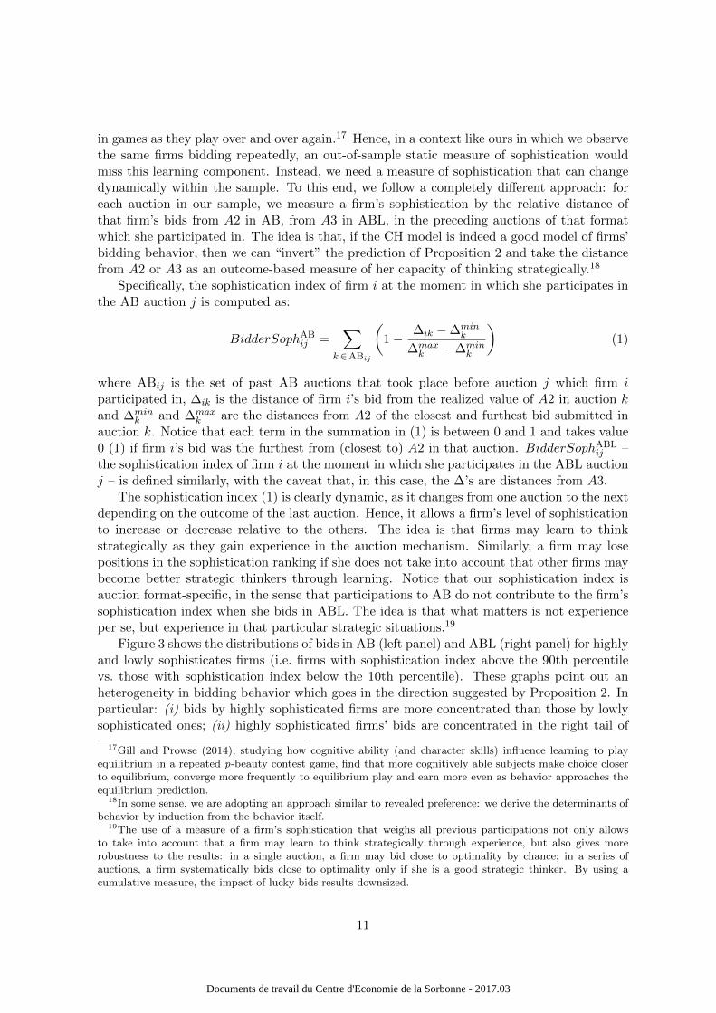
in games as they play over and over again.17 Hence, in a context like ours in which we observethe same firms bidding repeatedly, an out-of-sample static measure of sophistication wouldmiss this learning component. Instead, we need a measure of sophistication that can changedynamically within the sample. To this end, we follow a completely different approach: foreach auction in our sample, we measure a firm’s sophistication by the relative distance ofthat firm’s bids from A2 in AB, from A3 in ABL, in the preceding auctions of that formatwhich she participated in. The idea is that, if the CH model is indeed a good model of firms’bidding behavior, then we can “invert” the prediction of Proposition 2 and take the distancefrom A2 or A3 as an outcome-based measure of her capacity of thinking strategically.18

Specifically, the sophistication index of firm i at the moment in which she participates inthe AB auction j is computed as:

BidderSophABij =

∑k∈ABij

(1−

∆ik −∆mink

∆maxk −∆min

k

)(1)

where ABij is the set of past AB auctions that took place before auction j which firm iparticipated in, ∆ik is the distance of firm i’s bid from the realized value of A2 in auction kand ∆min

k and ∆maxk are the distances from A2 of the closest and furthest bid submitted in

auction k. Notice that each term in the summation in (1) is between 0 and 1 and takes value0 (1) if firm i’s bid was the furthest from (closest to) A2 in that auction. BidderSophABL

ij –the sophistication index of firm i at the moment in which she participates in the ABL auctionj – is defined similarly, with the caveat that, in this case, the ∆’s are distances from A3.

The sophistication index (1) is clearly dynamic, as it changes from one auction to the nextdepending on the outcome of the last auction. Hence, it allows a firm’s level of sophisticationto increase or decrease relative to the others. The idea is that firms may learn to thinkstrategically as they gain experience in the auction mechanism. Similarly, a firm may losepositions in the sophistication ranking if she does not take into account that other firms maybecome better strategic thinkers through learning. Notice that our sophistication index isauction format-specific, in the sense that participations to AB do not contribute to the firm’ssophistication index when she bids in ABL. The idea is that what matters is not experienceper se, but experience in that particular strategic situations.19

Figure 3 shows the distributions of bids in AB (left panel) and ABL (right panel) for highlyand lowly sophisticates firms (i.e. firms with sophistication index above the 90th percentilevs. those with sophistication index below the 10th percentile). These graphs point out anheterogeneity in bidding behavior which goes in the direction suggested by Proposition 2. Inparticular: (i) bids by highly sophisticated firms are more concentrated than those by lowlysophisticated ones; (ii) highly sophisticated firms’ bids are concentrated in the right tail of

17Gill and Prowse (2014), studying how cognitive ability (and character skills) influence learning to playequilibrium in a repeated p-beauty contest game, find that more cognitively able subjects make choice closerto equilibrium, converge more frequently to equilibrium play and earn more even as behavior approaches theequilibrium prediction.

18In some sense, we are adopting an approach similar to revealed preference: we derive the determinants ofbehavior by induction from the behavior itself.

19The use of a measure of a firm’s sophistication that weighs all previous participations not only allowsto take into account that a firm may learn to think strategically through experience, but also gives morerobustness to the results: in a single auction, a firm may bid close to optimality by chance; in a series ofauctions, a firm systematically bids close to optimality only if she is a good strategic thinker. By using acumulative measure, the impact of lucky bids results downsized.

11


Figure 3 – Discounts in AB (left panel) and ABL (right panel): Kernel density estimation byhighly and lowly sophisticated firms.

the distribution of bids in AB and in the left tail in ABL.20

Given that our sample contains (by far) more AB than ABL auctions, the average valueof the sophistication index is, by construction, larger in AB. Looking at the whole sample, thefrequency distribution of the index displays a higher concentration on low values and fewerobservations on high values in both formats, indicating that there are few highly sophisticated(firms that make good bids in a large number of auctions). However, looking only at lateyears, the distribution tends to be smoother, suggesting that, after some time, more and morefirms reach relatively high levels of their sophistication.21

4.2 Estimated equation

Given the measure of firms’ sophistication just illustrated, we can now introduce and esti-mate a reduced form model to test Proposition 2. The model is the following (we omit thedependence on the auction format, but it is intended that there is one such equation for eachformat):

log |Distanceij | = α+ β log(BidderSophij) + γFi + σFPij + θPj + εij . (2)

In (2), the dependent variable, log |Distanceij |, is the logarithm of the difference (in absolutevalue) between firm i’s bid in auction j and the realized value of A2 [A3] in that AB [ABL]auction. BidderSophij is firm i’s sophistication index at the moment of participation inauction j, as defined by (1).22 Fi represents a set of characteristics of firm i that do not vary

20A two-sample Kolmogorov-Smirnov test confirms that the distribution of bids by highly and lowly sophis-ticated firms are statistically different in both auction formats.

21See Figures D1 and D2 in Appendix D. See also Figure D3 in Appendix D, which shows the distributionof the sophistication index in AB auctions by firm size and period. Interestingly, distributions have similarshapes across firm sizes, although small firms reach lower levels of sophistication by the end of the period.

22We adopt a log-log model for two reasons: first, the theoretical analysis suggests a non-linear relationshipbetween sophistication and distance from A2 or A3; second, a log-log model allows to interpret the coefficientattached to the sophistication index as an elasticity. Notice that observations with a sophistication indexequal to zero are excluded as we require firms to show their bidding ability at least once before entering inthe analysis. Our main results do not change when we include firms with a sophistication index equal to zero

12


over time, including proxies for size and location.23 FPij is a set of firms’ characteristics thatcan vary for each auction. This set includes the backlog of works (i.e. the number of pendingpublic procurement projects a firm has at the moment she bids in auction j; it is a proxy forcapacity constraints) and the subcontracting position. Pj is a set of variables to control forthe characteristics of the auction, such as dimension and complexity of the auctioned work,24

and the timing of the auction (i.e. year dummy variables to adjust for temporal shocks to thefirms and the CA).

To reduce concerns about omitted variable problems affecting the relationship betweenthe sophistication index (which is built upon firms’ past behavior in auctions of that format)and firms’ current behavior (e.g., some factors that may influence both the past and currentperformance of firms are not controlled for), in some specifications we also included firm-fixedeffects to adjust for firm-specific characteristics. This enables us to focus on the within firmvariation in the sophistication status. However, some relevant characteristics of the firmscould vary over the time horizon of our analysis. For this reason, in some specifications wealso add firm-year-fixed effects, thus controlling for those characteristics which can vary overtime, like, for instance, productivity, financial position, and management skills. This set offixed effects represents a suitable substitute for the inclusion of firm-year control variablesthat can be recalled from balance-sheets.25

4.3 Description of the sample

Table 1 shows summary statistics of the sample used in our estimations, broken down byauction format.26 The sample of 232 AB auctions includes 8,927 bids made by 514 differentfirms; the sample of 28 ABL auctions includes 1,501 bids made by 319 different firms.27

(using log(1 + BidderSoph) as regressor) or when we adopt a log-linear specification (see Appendix D, TableD1).

23Because we do not have data on firms’ employees or total assets, we construct proxies for firms’ size basedon the type of business entity: Small = one-man businesses, limited and ordinary partnerships; Medium =limited liability companies; Large + cooperatives = public corporations and cooperatives. The use of theseproxies is motivated by the evidence of a positive correlation between the type of business entity and the sizeof Italian firms (see Moretti and Valbonesi, 2015, and Coviello et al., 2016). To proxy firms’ location, we takethe geographical distance between Aosta (i.e. the seat of the CA) and the chief town of the province where thefirm has her headquarter (we assign a distance of 30 kilometers to firms located in Valle d’Aosta, see Morettiand Valbonesi, 2015). This variable is also a proxy for firms’ costs (at least for the roadwork contracts, whichrepresent the majority of our auctions). We thank an anonymous referee for this comment.

24In the procurement literature, the complexity of a project is usually proxied by the its value or the auction’sreserve price, the expected contractual duration of works, dummies for the categories of works included in theproject. We use all these proxies in our estimation. Notice that the contract value is determined by an engineeremployed by the CA, according to a price list that enumerates the standardized costs for each type of work (seeDecarolis, 2014, and Coviello and Marinello, 2014, for details on how the CA determines this price). Similarly,the expected duration of the work is computed by a CA’s engineer and is stated in the call for tender.

25The presence of small and micro firms in our dataset makes it impossible for us to use balance-sheet infor-mation to construct additional controls or instrumental variables as these firms are typically under-representedin firm-level balance-sheet-based databases. In fact, a large number of firms is unmatched when we try to mergeour dataset with the Bureau Van Dijk’s Aida database of Italian firms.

26These descriptive statistics refer to the sample used for the empirical analysis proposed in this section. Theoriginal sample was slightly larger (267 auctions). The sophistication index is computed on this larger sampleto avoid being influenced by partial observations. However, due to missing values in some control variables,our regression analyses are based on the restricted sample.

27We thus rely on an unbalanced panel of firms. In the AB sample, on average, a firm participated in 18.4auctions: 17.32% of the firms participated in 2 auctions, 9.92% in 3 auctions, 6.42% in 4 auctions, 26.45% in

13


Table 1 – Estimated sample.

AB ABL

Obs. Mean SD Obs. Mean SD

Firm-auction level:

|Distance| 8927 1.555 2.437 1501 1.4333 1.990BidderSoph 8927 24.789 24.699 1501 4.192 3.954Backlog 8927 2.857 7.143 1501 2.005 4.963Optional Subcontracting 8927 0.871 0.336 1501 0.817 0.387

Auction level:

Reserve price (euro) 232 1,120,365 895,493.5 28 1,109,662 681,532.5Expected duration (days) 232 301.431 166.172 28 402.857 177.353No. Bidders 232 53.216 28.613 28 82.857 41.662Building construction 232 0.134 0.341 28 0.107 0.315Road works 232 0.388 0.488 28 0.286 0.460Hydraulic works 232 0.306 0.462 28 0.321 0.476

Firm level:

Small size 514 0.158 0.365 319 0.160 0.367Medium size 514 0.589 0.492 319 0.624 0.485Large size 514 0.253 0.435 319 0.216 0.412Distance firm-CA (km) 514 449.463 448.476 319 344.765 391.891

The average auction’s reserve price is around 1.1 million euros in both types of auctionsand the average number of participating firms per auction is about 53 in AB and 83 inABL. Most of the auctions concern road works (38.8% of the AB auctions; 28.6% of theABL auctions), hydraulic works (30.6% of the AB auctions; 32.1% of the ABL auctions)and building construction (13.4% of the AB auctions; 10.7% of the ABL auctions). The twosamples are pretty homogeneous also looking at firms’ other characteristics, such as size (about84% are medium or large firms), backlog (upon bidding, firms have, on average, between 2and 3 pending public procurement projects) and subcontracting position (on average, morethan 80% of the firms have the option to subcontract part of the work).

4.4 Main estimation result

In Table 2, columns (1)-(3), we present our estimation results for the sample of AB auctions.In all specifications, the negative and statistically significant coefficient of log(BidderSoph)shows that firms with a higher sophistication index tend to bid closer to A2, thus supportingthe prediction contained in Proposition 2. This result is robust to the inclusion of covariates atauction-, firm- and firm-auction-level (column (1)), firm-fixed effects (column (2)), and firm-year-fixed effects (column (3)). The inclusion of fixed effects allows us to explore the withinfirm (or firm-year) variability and to reduce selection-bias and omitted variable problems:in particular, firm-fixed effects can capture the role of any idyosincratic (either innate orpreviously acquired) component of sophistication peculiar to that firm/manager, while firm-year-fixed effects can capture this same component also for firms whose management changed

5-10 auctions, 28.74% in 11-50 auctions, 9.85% in 50-100 auctions, and 1.14% in more than 100 auctions. Inthe ABL sample, on average, a firm participated in 5.7 auctions: 28.53% of the firms participated in 2 auctions,19.44% in 3 auctions, 10.66% in 4 auctions, 26.65% in 5-10 auctions, and 14.74% in more than 10 auctions.

14


during the sample period.28

Table 2 – Main results.

Dependent variable log |Distance|Auction format AB AB AB ABL ABL ABL

(1) (2) (3) (4) (5) (6)

log(BidderSoph) -0.171*** -0.170*** -0.243*** -0.386*** -0.468*** -0.522***(0.022) (0.038) (0.041) (0.042) (0.063) (0.073)

Auction/project controls YES YES YES YES YES YESFirm controls YES NO NO YES NO NOFirm-FE NO YES NO NO YES NOFirm-year-FE NO NO YES NO NO YESFirm-auction controls YES YES YES YES YES YES

Observations 8,927 8,838 8,573 1,501 1,410 1,266R-squared 0.192 0.266 0.352 0.279 0.459 0.498

OLS estimations. Robust standard errors clustered at firm-level in parentheses.Inference: (***) = p < 0.01, (**) = p < 0.05, (*) = p < 0.1.Auction/project controls include: the auction’s reserve price, the expected duration of the work, dummy variables forthe type of work, dummy variables for the year of the auction. Firm controls include: dummy variables for the size ofthe firm, and the distance between the firm and the CA. Firm-auction controls include: a dummy variable for the firm’ssubcontracting position (mandatory or optional), and a measure of the firm’s backlog.

Table 2 also reports the results of the regressions for the sample of ABL auctions. Lookingat this sample is illuminating because it allows us not only to test the role of firms’ sophis-tication in a different average bid format, but also to address potential measurement errorproblems. In fact, while the AB format has long and widely been adopted in Italy to awardpublic works, the ABL format was introduced in 2006 and only in Valle d’Aosta. Hence, whilethe sophistication index computed for the AB sample does not take into account that firmsmay have gained experience (and thus sophistication) by participating in AB auctions issuedby other Italian CAs and/or in the past29, these measurement error concerns are absent inthe ABL case. Now, also the results for the ABL sample are consistent with Proposition 2:the relationship between sophistication index and the distance from A3 is highly significantand negative. This is true in all the specifications, without fixed effects (column (4)) and withfirm- or firm-year-fixed effects (columns (5) and (6)). Interestingly, the estimated coefficientfor the sophistication index in the ABL auctions indicate a larger negative effect than in AB.A plausible explanation for this could be related to the measurement error problems just dis-cussed. In fact, in AB auctions we might be underestimating the true level of sophisticationof firms, especially the most sophisticated ones, which are also those that are most likely tobid also outside Valle d’Aosta.30

28In Appendix D, Tables D1 and D2, we show that our main result is confirmed also when: (i) we replaceauction covariates with auction-fixed effects; (ii) we add the number of bidders as a proxy for the auction’scompetitive pressure; (iii) we estimate an Heckman selection model; (iv) the sophistication index is not onlyauction format- but also work category-specific (i.e. the sophistication acquired in one type of work is irrelevantwhen that firm bids in an auction for a different type of work).

29Anyhow, we believe that the impact of the experience gained outside Valle d’Aosta should be limitedbecause the knowledge of the specificity of each market (first of all, its players) is extremely important.Moreover, the sophistication accumulated in the past (i.e. before year 2000) should be captured by the fixedeffects.

30We thank an anonymous referee for suggesting this interpretation.

15


4.5 Learning dynamics

The previous analysis showed that, in line with the prediction obtained from a CH model,there is a stable negative relationship between firms’ sophistication index and the distanceof their bids from A2 or A3. However, that analysis does not say much about the dynamicsbehind this relationship. In particular, do firms learn to think and bid strategically as theyparticipate in more and more auctions? And, if so, what are the determinants and thecharacteristics of this learning process? Our starting point is the evidence suggested fromthe kernel density distribution of bids in AB auctions issued during the first (2000) and last(2005) year covered by our dataset. Figure 4 shows that, compared to year 2000, bids in 2005are generally much more concentrated on the right side of the distribution, thus suggestingthat a learning process is most likely to be taking place.

Figure 4 – Discounts in year 2000 and 2005: Kernel density estimation.

To investigate such process more in depth, we decompose firm i’s sophistication index atauction j into two components. The first component is simply the number of past partici-pations by firm i in auctions of the same format as j and is meant to capture the pure roleof experience; we denote this variable by PastPart. The second component is the averageperformance of firm i in all previous auctions of the same format as j, measured as the averagedistance of her bid from A2 or A3. This variable, denoted by PastPerf , is intended to proxythe degree at which a firm learns to think and bid strategically from her past performance.Furthermore, through the fixed effects at the firm-year level, we implicitly take into accountalso a third component: the stock of strategic skills of a firm/manager in any given year, bothinnate and acquired in the past.

Focusing on the sample of AB auctions, Table 3, column (1), shows the results obtainedby estimating a regression model like (2) with firm-year-fixed effects, where the regressorlog(BidderSoph) is replaced by log(PastPart). The latter has a negative and statisticallysignificant coefficient, showing that experience does play a role: everything else equal, firmsthat participate more bid better (i.e. closer to A2) than those that participate less. In column(2), we add log(1 + PastPerf) to the model specification: interestingly, its coefficient ispositive and significant, while the sign of log(PastPart) remains negative and statistically

16


significant. This evidence indicates that the main driver of a firm’s learning over time seemsto be the number of past bids and that, at least in AB auctions, a firm tends to learn morefrom a poor than from a good past performance, as if a poor performance acted as a stimulusfor the firm to improve her strategic reasoning in the future.

To get deeper evidence on the learning process we investigate whether the fact of winningan auction plays a role. To this end, we introduce the number of past wins (log(1+PastWins))in our model specification. Results for the AB auctions indicate that, similarly to whathappens with PastPerf , a firm seems to learn more from her failures than from her successes(see Table 3, columns (3) and (4)).31

The results for the ABL auctions32 confirm that the number of past participations posi-tively affect future bidding performance (the coefficient of log(PastPart) is always negativeand significant). However, differently from the AB sample, log(1 +PastPerf) has a negativesign (indicating that firms learn from their good past performances), which turns out to benonsignificant when firm-year fixed effects are included. Interestingly, log(1 + PastWins) inABL auctions is not statistically significant. This is probably not surprising, as the winner inan ABL auction is determined randomly: hence, the fact of winning produces less informationthan in the AB format.

To sum up, the learning process seems to be mainly driven by pure experience: firmsimprove their capacity of bidding strategically as they participate to more and more auctions.Instead, the performance in past auctions has little explanatory power: once firms’ idiosyn-cratic skills are controlled for (through the fixed effects), a better average performance or alarger number of wins in the past either has no impact on bidding behavior in future auctions(in ABL) or worsens the capacity of bidding optimally (AB), as if it acted as a negativestimulus to improve strategic thinking. This analysis also allows us to exclude that the re-lationship we uncovered between the sophistication index and bidding performance is simplydue to inertia in bidding over time: firms learn how to bid strategically through experience,so those firms that participate more can eventually become more sophisticated than thosethat participate less, even if the latter were better strategic thinkers initially.

Given the peculiarity of our dataset characterized by a change in the auction format, andgiven the results about the learning dynamics just illustrated, it is interesting to understandwhether firms in ABL auctions drew lessons from what they learned in the AB auctions (in oursample, 240 firms participated both in AB and ABL auctions). Recall that our sophisticationindex was, by construction, auction format-specific, in the sense that participations to AB donot contribute to firms’ sophistication when they bid in ABL. Hence, answering this question isan indirect way to test how restrictive this assumption is. To this end, we focus on the sampleof ABL auctions and introduce in our model (2) an additional variable, BidderSophAB,representing, for each firm, the level of the sophistication index at the end of the period ofAB auctions. Table 3, column (5), shows that a higher sophistication index achieved in theAB period is associated with a lower distance from A3 in ABL. However, when we re-introduce(in column (6)) the firm’s sophistication associated to the ABL auctions (BidderSoph), thecoefficient of the former index is not statistically different from zero, while the auction-specificone is still negative and statistically significant. This result suggests that what really matters

31Notice that, in a specification without firm-year- (or firm-) fixed effects, the interpretation of the coefficientis different: negative coefficients of both log(1 + PastPerf) and log(1 + PastWins) indicate that, betweenfirms, those with better past performance tend to consistently bid closer to the reference point than those withworse past performance. See Appendix D, Table D3.

32These results are reported Appendix D, Table D4.

17


Table 3 – Learning dynamics.

Dependent variable log |Distance|Auction format AB AB AB AB ABL ABL ABL ABL

(1) (2) (3) (4) (5) (6) (7) (8)log(PastPart) -0.366*** -0.442*** -0.505***

(0.044) (0.048) (0.054)log(1+PastPerf) 5.018*** 4.937***

(0.732) (0.729)log(1+PastWins) 0.624*** 0.555***

(0.173) (0.164)log(BidderSoph) -0.293*** -0.412*** -0.409***

(0.046) (0.045) (0.047)log(BidderSophAB) -0.088** -0.008

(0.039) (0.042)log(PastPartAB) -0.063 0.013

(0.041) (0.046)log(1+PastPerfAB) -1.741** -1.297

(0.836) (0.811)Auction/project controls YES YES YES YES YES YES YES YESFirm controls NO NO NO NO YES YES YES YESFirm-year-FE YES YES YES YES NO NO NO NOFirm-auction controls YES YES YES YES YES YES YES YESObservations 8,573 8,573 8,573 8,573 1,356 1,356 1,356 1,356R-squared 0.354 0.362 0.364 0.353 0.231 0.284 0.234 0.286

OLS estimations. Robust standard errors clustered at firm-level in parentheses.Inference: (***) = p < 0.01, (**) = p < 0.05, (*) = p < 0.1.Auction/project controls include: the auction’s reserve price, the expected duration of the work, dummy variables forthe type of work, dummy variables for the year of the auction. Firm controls include: dummy variables for the size ofthe firm, and the distance between the firm and the CA. Firm-auction controls include: a dummy variable for the firm’ssubcontracting position (mandatory or optional), and a measure of the firm’s backlog.

is the firm’s strategic ability acquired in that specific type of auction.Similar results are obtained when we introduce in the model specification the number

of participations (PastPartAB) and the average past performance (PastPerfAB) in ABauctions (columns (7) and (8)). The coefficients of these two variables are not significant,once we control for the ability acquired by the firm in the ABL auctions.

5 Discussion

The analysis presented in the previous section provides evidence that supports, at least qual-itatively, a non-equilibrium model of bidding behavior by firms in average bid auctions: ob-served deviations from the optimal bid are related to a measure of firms’ capacity of biddingstrategically, the sophistication index; this relation goes in the direction predicted by a CHmodel. Therefore, our (continuous) sophistication index proxies the (discrete) CH-level ofsophistication by firms. The analysis showed that the relation between sophistication indexand bidding behavior is robust to a number of determinants, including auction’s, firm’s andfirm-auction’s specific characteristics. Most importantly, the relation holds also when we an-alyze the ABL format, which is new to the firms and characterized by a stochastic componentthat makes it more complicated for firms to formulate their bidding strategies.

In this section, we show that our explanation is robust to a number of issues that, po-tentially, may undermine it. In particular, we discuss: (i) whether our sophistication index,which we interpret as a measure of strategic thinking ability, may be actually capturingother firms’ structural factors, in particular their competitiveness; (ii) the role of potential

18


cartels jointly bidding in the auctions; (iii) an instrumental variable approach to deal withendogeneity problems; (iv) additional empirical evidence to rule out alternative explanations.

5.1 Strategic ability vs. competitiveness

In standard procurement auctions, the main determinant of a firm’s bid is her production cost:more competitive firms can and do make more aggressive offers, outbidding less competitiveones. A natural question that arises in our context is whether our sophistication index, which,in our view, proxies strategic ability, actually captures some structural competitive feature ofthe firm: productivity, proximity, or, more generally, any element that translates into a costadvantage. Now, notice first that, in our main empirical exercise, we alternatively control forfirm’s characteristics (such as size and distance between the firm headquarter and the CA),firm-fixed, or firm-year-fixed effects, as well as for the firm’s subcontracting position (whetherthe firm must subcontract part of the work or not) and for the number of pending projects thefirm is involved in at the time of bidding (which captures her productive capacity).33 Mostfactors that may generate a competitive advantage/disadvantage of one firm over the othersare likely to be accounted for by these variables.

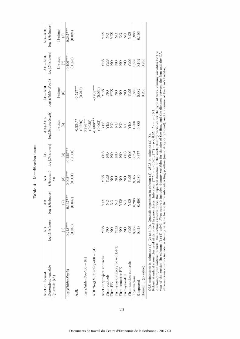
However, one might argue that we do not fully control for factors that, similarly to thesophistication index, can vary for each firm within a year or for different types of project. Toshed light on these questions, we first estimated a model which includes firm-year-category ofwork-fixed effects and one with firm-semester-fixed effects: in both models, the coefficient oflog(BidderSoph) in AB auctions is very much in line with that of our main model specification(see Table 4, columns (1) and (2).34

33Jofre-Bonet and Pesendorfer (2003), using a dataset of a sequence of first-price procurement auctions forhighway construction in California, showed that the outcome of one auction may affect bids in successive onesbecause the winner of a previous auction, having committed some or all of her capacity, may have larger costswhen participating in the next auctions (because, for example, it will have to rent additional equipment). Inour context, this dynamic component seems to be absent, as the variable Backlog – the number of pendingpublic procurement projects that a firm has at the moment of bidding – is never significant. Our intuition isthat, even though it is plausible that having committed capacity can affect firms’ costs, costs simply do notmatter much for (optimal) bidding in average bid auctions.

34Our result is robust also to the inclusion of firm-semester-category of work-fixed effects. Due to the smallersample dimension, results are slightly weaker for the ABL format (see Appendix D, Table D5).

19


Tab

le4

–Id

enti

fica

tion

issu

es.

Auct

ion

form

at

AB

AB

AB

AB

AB

+A

BL

AB

+A

BL

AB

+A

BL

AB

+A

BL

Dep

enden

tva

riable

log|Distance|

log|Distance|

Discount

log|Distance|

log(BidderSoph

)lo

g(BidderSoph

)lo

g|Distance|

log|Distance|

Quanti

le(th

)90

I-st

age

I-st

age

II-s

tage

II-s

tage

(1)

(2)

(3)

(4)

(5)

(6)

(7)

(8)

log(BidderSoph

)-0

.243***

-0.1

37***

-0.0

03***

-0.2

28***

-0.1

96***

-0.2

37***

(0.0

45)

(0.0

47)

(0.0

01)

(0.0

60)

(0.0

23)

(0.0

24)

AB

L-0

.534**

-0.5

27**

(0.2

26)

(0.2

13)

log(BidderSoph

00−

04)

0.7

86***

(0.0

38)

AB

L*lo

g(BidderSoph

00−

04)

-0.6

88***

-0.7

05***

(0.0

62)

(0.0

60)

Auct

ion/pro

ject

contr

ols

YE

SY

ES

YE

SY

ES

YE

SY

ES

YE

SY

ES

Fir

mco

ntr

ols

NO

NO

YE

SN

OY

ES

NO

YE

SN

OF

irm

-FE

NO

NO

NO

NO

NO

YE

SN

OY

ES

Fir

m-y

ear-

cate

gory

of

work

-FE

YE

SN

ON

ON

ON

ON

ON

ON

OF

irm

-sem

este

r-F

EN

OY

ES

NO

NO

NO

NO

NO

NO

Fir

m-y

ear-

FE

NO

NO

NO

YE

SN

ON

ON

ON

OF

irm

-auct

ion

contr

ols

YE

SY

ES

YE

SY

ES

YE

SY

ES

YE

SY

ES

Obse

rvati

ons

8,0

68

8,2

08

8,9

27

3,5

94

1,8

88

1,8

88

1,8

88

1,8

88

R-s

quare

d0.4

13

0.4

08

0.1

89

0.3

77

0.8

88

0.8

82

0.1

02

0.1

06

Hanse

nJ

(p-v

alu

e)0.2

56

0.2

85

OL

Ses

tim

ati

on

sin

colu

mn

s(1

),(2

)an

d(4

).Q

uanti

lere

gre

ssio

nin

colu

mn

(3).

2S

LS

inco

lum

ns

(5)-

(8).

Rob

ust

stan

dard

erro

rscl

ust

ered

at

firm

-lev

elin

pare

nth

eses

.In

fere

nce

:(*

**)

=p<

0.0

1,

(**)

=p<

0.0

5,

(*)

=p<

0.1

.Auction/project

controls

incl

ud

e:th

eau

ctio

n’s

rese

rve

pri

ce,

the

exp

ecte

dd

ura

tion

of

the

work

,d

um

my

vari

ab

les

for

the

typ

eof

work

,d

um

my

vari

ab

les

for

the

yea

rof

the

au

ctio

n(i

nco

lum

ns

(1)-

(4)

on

ly).

Firm

controls

incl

ud

e:d

um

my

vari

ab

les

for

the

size

of

the

firm

,an

dth

ed

ista

nce

bet

wee

nth

efi

rman

dth

eC

A.

Firm-auctioncontrols

incl

ud

e:a

dum

my

vari

ab

lefo

rth

efi

rm’s

sub

contr

act

ing

posi

tion

(man

dato

ryor

opti

on

al)

,an

da

mea

sure

of

the

firm

’sb

ack

log.

20


Second, we performed an analysis on the level of bids. We start from the conjecture that,if our sophistication index were actually capturing some cost advantage, we would expect toobserve either a positive or a null relation between the sophistication index and the level ofa firm’s bid. In fact, irrespective of the auction format and of the submitted bid, if a firm’scosts are binding (in the sense that, had her costs been lower, she would have made a differentbid), a cost reduction would necessarily result in a higher bid; if, instead, her costs are notbinding, a further cost reduction should have no impact on her bid. On the other hand, ifour sophistication index captures strategic ability, as we claim, we would expect to observea negative [positive] relationship between the sophistication index and the bid level for firmsmaking relatively high [low] bids. In fact, in average bid auctions, an improvement in strategicability would lead firms that bid too high [low] to reduce [increase] their bids towards theoptimal bid, which is necessarily somewhere in the interior of the range of submitted bids.Now, focusing on the AB sample, our evidence is indeed in line with the latter interpretationand inconsistent with the one based on cost advantage: the effect of the sophistication indexon the level of bids, though nonsignificant overall, is negative and significant for those firmsbidding the highest (see the result of the regression at the 90-th quantile in Table 4, column(3)). 35

5.2 Potential collusion

A very interesting aspect that is worth addressing is related to possible collusive behaviorsby firms. In a recent paper, Conley and Decarolis (2016), using a different dataset of ABauctions, argue that this format can be characterized by the presence of colluding firms whichdrive the winning threshold to let one member of the cartel win. Hence, the evidence onAB auctions would be the result of a cooperative behavior by groups of firms. Instead, ourapproach is totally different: we cannot exclude the presence of colluding firms, but we providesome evidence that also a fully non-cooperative non-equilibrium behavior might be at work.In this sense, our work suggests a complementary explanation. Nevertheless, we can providesome arguments supporting the robustness of our findings to the presence of collusion. First,it seems reasonable to assert that, if collusion is at work, it is less likely to be present in ABLthan in AB auctions: given the inherent uncertainty in the determination of the winningfirm, in ABL a successful collusive strategy is much more complicated to be implemented.In this sense, the fact that the coefficient of the sophistication index is significant also inABL and larger than in AB (see Table 2) is reassuring for our explanation. Second, withoutany intention to provide evidence on the presence of cartels in the auctions issued by theRegional Government of Valle d’Aosta (note that, unlike in Conley and Decarolis, in oursample no cartels have been detected and sanctioned by the court; this makes more difficultto study possible collusive behavior in our setting), we tried to isolate the influence of potentialcollusive groups. To this end, we identified potential cartels following Conley and Decarolis(2016). In particular, using information on objective links among firms (e.g., firms sharing thesame managers, the owners, the location, subcontracting relationship, joint bidding, etc.), theConley and Decarolis’ algorithm indicates that, in our sample, 172 potential groups of firmsare present. Once detected these groups, we included in our baseline model specification two

35See Appendix D, Tables D6 and D7, for evidence on ABL auctions and further evidence at differentquantiles of the distribution of bids. Notice that, in both formats, the coefficients of the sophistication indexin the quantile regressions exactly match the pattern predicted by a CH model: they are negative [positive]and statistically significant for high [low] bid levels.

21


variables measuring, for each firm and each auction: (i) the number of (potentially) associatedfirms bidding in that auction; (ii) this number over the total number of firms belonging tothat group. Our main results continue to hold after the inclusion of these controls.36 Itmust anyway be observed that data display a (weak) positive correlation between our indexof sophistication and the number of (potentially) associated firms bidding in that auction,both in AB (0.144) and in ABL (0.188) auctions. Moreover, independent firms – those withno potential associate in the auction – show, on average, lower sophistication than associatedfirms (the difference is about 35% in AB and 45% in ABL): these numbers may suggestthat, if cartels are present, their members are typically more sophisticated than independentfirms. Now, to better isolate the role of potential collusion from that of strategic ability, weestimated our baseline model on a restricted sample including only firms with no connectionwith any other firm participating in that auction (Table 4, column (4)). Again, our mainresult is confirmed, thus supporting the idea that our explanation actually captures biddingbehavior by firms, at least for those that act non-cooperatively.

5.3 Instrumental variables

The results presented so far are robust to the inclusion of rich sets of fixed effects and con-trol variables in the estimated equation. However, to further address potential endogeneityconcerns, we also consider an instrumental variable (IV) approach, aimed at capturing someexogenous components behind the sophistication index. Given that information on severalrelevant firms’ characteristics (such as information coming from balance-sheets or managerialand organizational structure of the firm) is not available, we choose an approach that jointlycombines out-of-sample information and the exogenous change of format from AB to ABL.

In particular, our identification strategy works as follows. First, we limit our analysis toyear 2005 and 2006, the last year of adoption of the AB format and the first year of adoptionof the ABL format, respectively. Focusing on such a short period of time, we can reduceomitted variable problems and exploit the 2006 variation in the auction format, which, it isworth recalling, took place only in Valle d’Aosta. Second, we consider three instrumentalvariables for the sophistication index, namely: (i) the dummy variable ABL (which takesvalue equal 1 for ABL and 0 for AB) to capture the average overall change in the firms’sophistication level determined by the change of format; (ii) for each firm, the value of hersophistication index at the end of 2004 (BidderSoph00-04 ), a proxy for the firm-fixed levelof sophistication (relative to the others) acquired out-of-sample; (iii) the interaction betweenthe previous two variables, which accounts for possibly differential effects that the new ABLformat had on firms’ current sophistication across firms with different levels of past (andout-of-sample) sophistication.

First-stage estimation results, reported in Table 4 column (5), show that the coefficientsof the three instruments are statistically different from zero (the Hansen J-test reported incolumn (8) confirms the validity of the instruments). The signs of the coefficients indicatethat: (i) the change of format reduced the overall level of bidders’ sophistication (since thesophistication index is specific for each auction format); (ii) the higher the firm’s past (andout-of-sample) sophistication in AB auctions, the higher her level of current sophistication inAB auctions (confirming that experience and past performance have an effect over time withinthe same auction format); (iii) the heterogeneity in sophistication across firms recorded at

36Estimation results for this analysis are available in Appendix D, Tables D8 and D9. We really thankFrancesco Decarolis for providing us with his codes and data.

22


the end of 2004 is greatly reduced when the new ABL format has been adopted. The resultsof the second-stage estimation (column (7)) confirm a negative and significant relationshipbetween the instrumented current level of sophistication of the firm and the distance of herbids from A2 in AB and A3 in ABL. Notice that these results are robust to the inclusion offirm-fixed effects (Table 4, columns (6) and (8)).37 Notice also that we control for severalauction’s characteristics (such as typology, value and duration of the work), thus reducing thepossibility that our instruments affect firms’ bidding behavior through other channels thansophistication.

5.4 Further evidence

Beyond the main result that more sophisticated firms bid closer to A2 in AB, to A3 in ABL,there is additional evidence that supports our interpretation, in the sense that it can easilybe reconciled within a CH model, much less so within an alternative explanation.38

First, notice that firms make relatively lower bids in ABL than in AB: this is clear fromour data (see Figure 2); furthermore, if we run a regression on a sample of (min-max rescaled)bids offered both in AB and ABL auctions (taking all the covariates included in equation (2)),the coefficient for the ABL auction dummy is negative and statistically significant.39 Now,if firms were making equilibrium bids, we should observe the opposite (see Proposition 1);instead, in a CH model, given the behavior of level-0 firms, bids made by firms of higher levelsare larger in AB than in ABL, since, by definition, A2k, the (asymptotically) optimal bid bya level-(k + 1) firm in AB, is larger than A3k.

Second, data show that not only the average distance from A2 or A3 is decreasing in thefirm’s sophistication level, but also the variance of this distance follows the same pattern.In fact, running a regression where the dependent variable is the standard deviation of thedistance of the auction’s bids from A2 or A3, the coefficient of the auction’s average sophisti-cation index is negative and significant in both formats. Moreover, in a regression where thedependent variable is the rolling standard deviation of the distance of a firm’s latest five bidsfrom A2 or A3, the coefficient of the firm’s rolling average sophistication index is negative andsignificant, even when firm-fixed effects are controlled for. Now, while there is no particularreason to expect a relationship between variance of bidding and other firm’s characteristics(e.g. her production costs), a negative relationship between sophistication index and varianceof bidding can be justified within a CH model with at least three arguments. First, in a CHmodel, level-0 firms bid randomly, while more sophisticated firms bid (essentially) determin-istically. Second, if firms make some payoff-sensitive errors,40 then more sophisticated firmswill make more precise bids (with less variance). The intuition is simple: to compute her

37In Appendix D, Table D10, we show similar estimation results after enlarging the sample of auctions tothe period 2004-2007.

38This evidence is collected in Appendix D, Table D11.39Notice that, even if we cannot fully separate in a difference-in-differences style the trend forces from the

effects related to the introduction of the (new) ABL auction format in Valle d’Aosta (as we do not observeAB auctions after 2005), evidence based on a larger sample of procurement auctions (data from Coviello etal., 2016) indicate that, for other Italian regions not adopting the ABL auction format, the average winningdiscount in 2006 is approximately at the same level as in 2005 or it has increased for some Northwestern regions.Given that, between 2005 and 2006, no major changes occurred in in Valle d’Aosta’s economy conditions andin the procurement regulation (other than the introduction of ABL auction format), we can assume that, hadValle d’Aosta not introduced the ABL auction, the trend would have followed a nondecreasing path similar tothe one observed in the other regions.

40See the simulation exercise in Appendix C.

23


optimal bid, a level-k firm estimates the distribution of the winning threshold on the basis ofthe behaviors of level-0 to level-(k−1) firms. For higher level firms, this distribution has lowervariance, being less and less affected by the random behavior of level-0 firms. Third, as itseems reasonable, more sophisticated firms may be less prone to errors than less sophisticatedones.

Third, data show that the higher the number of participating firms in an auction, thehigher [the lower] the value of A2 [A3] in AB [ABL]. This can be seen by looking at descriptivestatistics (the simple correlation between the number of participants and A2 [A3] in AB [ABL]is positive [negative]) and by estimating a regression with A2 or A3 as the dependent variableand the number of participants and other auction-level controls as regressors. This evidenceis consistent with a CH model of bidding behavior: in the viewpoint of a sophisticated firm,who determines her bid on the basis of her own estimates of the distribution of A2 or A3, alower number of participants increases the variance of this distribution. Since the winning bidis the one that gets closer to the winning threshold from below in AB and from above in ABL,a sophisticated firm will find it optimal to bid cautiously: in AB, a little below the expectedvalue of A2, in ABL a little above the expected value of A3. As the number of participantsincreases, the variance of A2 or A3 will reduce, and sophisticated firms can be more confidentin bidding very close to their expected values.

6 Conclusion

This paper studies bidding behavior by firms in two versions of average bid auctions adoptedby a regional contracting authority in Italy for the procurement of public works. Our empiricalevidence is inconsistent with Nash equilibrium behavior, a situation in which all firms areplaying their best response to other firms’ bids. We proposed an interpretation based ona non-equilibrium CH model of bidding behavior: more sophisticated firms, being betterstrategic thinkers, are able to get more accurate beliefs on the behavior of other firms andbid closer to optimality. Introducing a dynamic measure of sophistication which takes intoaccount the goodness of a firm’s bids in all past auctions of the same format in our sample,we showed that the main prediction of the CH model is consistent with our data. We alsoinvestigated whether and how firms learn to think and bid strategically through experience,showing that both the number of participations and the average past performance explainfirms’ performance in future auctions and that this learning process has a convergence path.We finally discussed endogeneity issues and alternative explanations for the observed behaviorin the investigated setting (in particular, collusion) by providing some robustness checks onour empirical analysis.

The general lesson that can be learned from our work is twofold. First, our paper providesevidence that departures from equilibrium can be significant and persistent also in the field,and even when players are firms and stakes are large. This is likely to be the case especially incomplex environments, for example when the profit of one firm depends in a non-obvious wayon the decisions made by all other firms. In this case, the equilibrium requirement that allplayers (firms) have correct beliefs seems particularly, and maybe unrealistically, demanding.

Second, the CH model and, more generally, models that take into account that strategicthinking may be heterogeneously distributed across economic agents, represent a valid alter-native to equilibrium models in complex games, even outside the lab. Moreover, while inthe experimental literature on CH models, convergence to equilibrium is usually observed, so

24


that CH models mainly capture initial responses to games, our evidence shows that, even ifconvergence is taking place, it does so at a slow rate. This is not surprising once one takesinto account that, unlike in the lab, in the field the set of players can change continuously overtime: new unexperienced firms may enter the stage, others may exit. Hence, even thoughexperience may help firms become more sophisticated, the entry of unsophisticated firms mayslow down the process of convergence.

References

[1] Albano, G., Bianchi, M., Spagnolo, G., 2006. Bid Average Methods in Procurement.Rivista di Politica Economica 1-2, 41-62.

[2] Branas-Garza, P., Garcıa-Munoz, T., Hernan Gonzales, R., 2012. Cognitive effort in thebeauty contest game. Journal of Economic Behavior and Organization, 83: 254-260.

[3] Brown, A.L., Camerer, C.F., Lovallo, D., 2012. To review or not to review? Limitedstrategic thinking at the movie box office. American Economic Journal: Microeconomics 4,1-26.

[4] Bucciol, A., Chillemi, O., Palazzi, G., 2013. Cost overrun and auction format in small sizepublic works. European Journal of Political Economy 30, 35-42.

[5] Burnham, T.C., Cesarini, D., Johannesson, M., Lichtenstein, P., Wallace, B., 2009. Highercognitive ability is associated with lower entries in a p-beauty contest. Journal of EconomicBehavior and Organization 72, 171-175.

[6] Camerer, C.F., Ho, T.H., Chong, J.K., 2004. A cognitive hierarchy model of games.Quarterly Journal of Economics 119, 861-898.

[7] Cameron, L.J., 2000. Limiting buyer discretion: effects on performance and price in long-term contracts. American Economic Review 90, 265-281.

[8] Chang, W.S., Chen, B., Salmon, T.C., 2015. An investigation of the average bid mecha-nism for procurement auctions. Management Science 61, 1237-1254.

[9] Chen, S.H., Du, Y.R., Yang, L.X., 2014. Cognitive capacity and cognitive hierarchy: astudy based on beauty contest experiments. Journal of Economic Interaction and Coordi-nation 9, 69-105.

[10] Conley, T., Decarolis, F., 2016. Detecting bidders groups in collusive auctions. AmericanEconomic Journal: Microeconomics 8, 1-38.

[11] Coviello, D., Moretti, L., Spagnolo, G., Valbonesi, P., 2016. Court efficiency and pro-curement performance. Scandinavian Journal of Economics, forthcoming.

[12] Coviello, D., Mariniello, M., 2014. Does publicity affect competition? Evidence fromdiscontinuities in public procurement auctions. Journal of Public Economics 109, 609-623.

[13] Crawford, V.P., Costa-Gomes, M.A., Iriberri, N., 2013. Structural models of nonequilib-rium strategic thinking: theory, evidence, and applications. Journal of Economic Literature51, 5-62.

25


[14] Crawford, V.P., Iriberri, N., 2007. Level-k auctions: can a nonequilibrium model ofstrategic thinking explain the winner’s curse and overbidding in private-value auctions?Econometrica 75, 1721-1770.

[15] Decarolis, F., 2009. When the highest bidder loses the auction:theory and evidence frompublic procurement. Bank of Italy Working Paper 717.

[16] Decarolis, F., 2014. Awarding price, contract performance, and bids screening: evidencefrom procurement auctions. American Economic Journal: Applied Economics 6, 108-132.

[17] Gil, R., Marion, J., 2013. Self-enforcing agreements and relational contracting: evidencefrom California highway procurement. Journal of Law, Economics, and Organization 29,239-277.

[18] Gill, D., Prowse, M., 2014. Cognitive ability, character skills, and learning to play equi-librium: a level-k analysis. Journal of Political Economy, forthcoming.

[19] Gillen, B.J., 2009. Identification and estimation of level-k auctions. Available at SSRN:http://ssrn.com/abstract=1337843 or http://dx.doi.org/10.2139/ssrn.1337843.

[20] Goldfarb, A., Yang, B., 2009. Are all managers created equal? Journal of MarketingResearch 46, 612-622.

[21] Goldfarb, A., Xiao, M., 2011. Who thinks about the competition? Managerial ability andstrategic entry in US local telephone markets. American Economic Review 101, 3130-3161.

[22] Jofre-Bonet, M., Pesendorfer, M., 2003. Estimation of a dynamic auction game. Econo-metrica 71, 1443-1489.

[23] Moretti, L., Valbonesi, P., 2015. Firms’ qualifications and subcontracting in public pro-curement: an empirical investigation. Journal of Law, Economics, and Organization 31,568-598.

[24] Nagel, R., 1995. Unraveling in guessing games: an experimental study. American Eco-nomic Review 85, 1313-1326.

[25] Stahl, D.O., Wilson, P.W., 1994. Experimental evidence on players’ models of otherplayers. Journal of Economic Behavior and Organization 25, 309-327.

[26] Stahl, D.O., Wilson, P.W., 1995. On players’ models of other players: theory and exper-imental evidence. Games and Economic Behavior 10, 218-254.

[27] Zheng, C., 2001. High bids and broke winners. Journal of Economic Theory 100, 129-171.

26


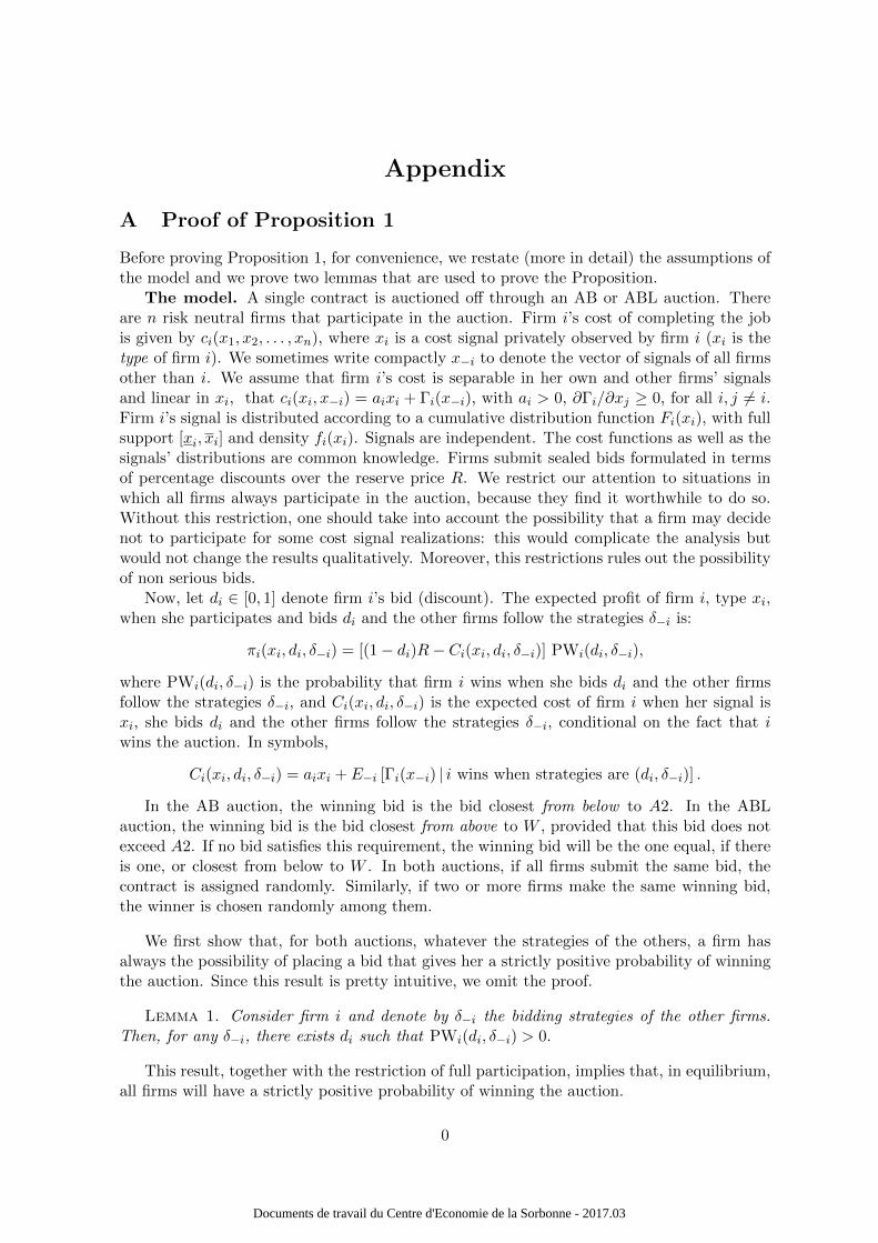
Appendix

A Proof of Proposition 1

Before proving Proposition 1, for convenience, we restate (more in detail) the assumptions ofthe model and we prove two lemmas that are used to prove the Proposition.

The model. A single contract is auctioned off through an AB or ABL auction. Thereare n risk neutral firms that participate in the auction. Firm i’s cost of completing the jobis given by ci(x1, x2, . . . , xn), where xi is a cost signal privately observed by firm i (xi is thetype of firm i). We sometimes write compactly x−i to denote the vector of signals of all firmsother than i. We assume that firm i’s cost is separable in her own and other firms’ signalsand linear in xi, that ci(xi, x−i) = aixi + Γi(x−i), with ai > 0, ∂Γi/∂xj ≥ 0, for all i, j 6= i.Firm i’s signal is distributed according to a cumulative distribution function Fi(xi), with fullsupport [xi, xi] and density fi(xi). Signals are independent. The cost functions as well as thesignals’ distributions are common knowledge. Firms submit sealed bids formulated in termsof percentage discounts over the reserve price R. We restrict our attention to situations inwhich all firms always participate in the auction, because they find it worthwhile to do so.Without this restriction, one should take into account the possibility that a firm may decidenot to participate for some cost signal realizations: this would complicate the analysis butwould not change the results qualitatively. Moreover, this restrictions rules out the possibilityof non serious bids.

Now, let di ∈ [0, 1] denote firm i’s bid (discount). The expected profit of firm i, type xi,when she participates and bids di and the other firms follow the strategies δ−i is:

πi(xi, di, δ−i) = [(1− di)R− Ci(xi, di, δ−i)] PWi(di, δ−i),

where PWi(di, δ−i) is the probability that firm i wins when she bids di and the other firmsfollow the strategies δ−i, and Ci(xi, di, δ−i) is the expected cost of firm i when her signal isxi, she bids di and the other firms follow the strategies δ−i, conditional on the fact that iwins the auction. In symbols,

Ci(xi, di, δ−i) = aixi + E−i [Γi(x−i) | i wins when strategies are (di, δ−i)] .

In the AB auction, the winning bid is the bid closest from below to A2. In the ABLauction, the winning bid is the bid closest from above to W , provided that this bid does notexceed A2. If no bid satisfies this requirement, the winning bid will be the one equal, if thereis one, or closest from below to W . In both auctions, if all firms submit the same bid, thecontract is assigned randomly. Similarly, if two or more firms make the same winning bid,the winner is chosen randomly among them.

We first show that, for both auctions, whatever the strategies of the others, a firm hasalways the possibility of placing a bid that gives her a strictly positive probability of winningthe auction. Since this result is pretty intuitive, we omit the proof.

Lemma 1. Consider firm i and denote by δ−i the bidding strategies of the other firms.Then, for any δ−i, there exists di such that PWi(di, δ−i) > 0.

This result, together with the restriction of full participation, implies that, in equilibrium,all firms will have a strictly positive probability of winning the auction.

0


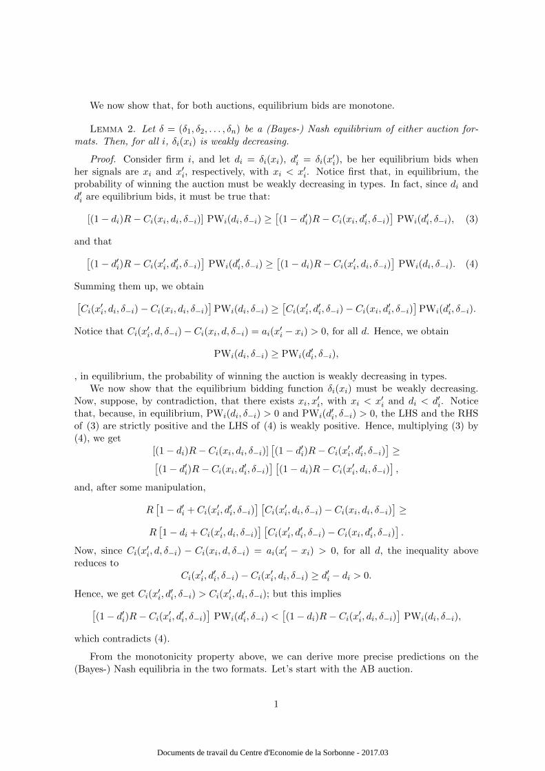
We now show that, for both auctions, equilibrium bids are monotone.

Lemma 2. Let δ = (δ1, δ2, . . . , δn) be a (Bayes-) Nash equilibrium of either auction for-mats. Then, for all i, δi(xi) is weakly decreasing.

Proof. Consider firm i, and let di = δi(xi), d′i = δi(x

′i), be her equilibrium bids when

her signals are xi and x′i, respectively, with xi < x′i. Notice first that, in equilibrium, theprobability of winning the auction must be weakly decreasing in types. In fact, since di andd′i are equilibrium bids, it must be true that:

[(1− di)R− Ci(xi, di, δ−i)] PWi(di, δ−i) ≥[(1− d′i)R− Ci(xi, d

′i, δ−i)

]PWi(d

′i, δ−i), (3)

and that[(1− d′i)R− Ci(x

′i, d′i, δ−i)

]PWi(d

′i, δ−i) ≥

[(1− di)R− Ci(x

′i, di, δ−i)

]PWi(di, δ−i). (4)

Summing them up, we obtain[Ci(x

′i, di, δ−i)− Ci(xi, di, δ−i)

]PWi(di, δ−i) ≥

[Ci(x

′i, d′i, δ−i)− Ci(xi, d

′i, δ−i)

]PWi(d

′i, δ−i).

Notice that Ci(x′i, d, δ−i)− Ci(xi, d, δ−i) = ai(x

′i − xi) > 0, for all d. Hence, we obtain

PWi(di, δ−i) ≥ PWi(d′i, δ−i),

, in equilibrium, the probability of winning the auction is weakly decreasing in types.We now show that the equilibrium bidding function δi(xi) must be weakly decreasing.

Now, suppose, by contradiction, that there exists xi, x′i, with xi < x′i and di < d′i. Notice

that, because, in equilibrium, PWi(di, δ−i) > 0 and PWi(d′i, δ−i) > 0, the LHS and the RHS

of (3) are strictly positive and the LHS of (4) is weakly positive. Hence, multiplying (3) by(4), we get

[(1− di)R− Ci(xi, di, δ−i)][(1− d′i)R− Ci(x

′i, d′i, δ−i)

]≥[

(1− d′i)R− Ci(xi, d′i, δ−i)

] [(1− di)R− Ci(x

′i, di, δ−i)

],

and, after some manipulation,

R[1− d′i + Ci(x

′i, d′i, δ−i)

] [Ci(x

′i, di, δ−i)− Ci(xi, di, δ−i)

]≥

R[1− di + Ci(x

′i, di, δ−i)

] [Ci(x

′i, d′i, δ−i)− Ci(xi, d

′i, δ−i)

].

Now, since Ci(x′i, d, δ−i) − Ci(xi, d, δ−i) = ai(x

′i − xi) > 0, for all d, the inequality above

reduces toCi(x

′i, d′i, δ−i)− Ci(x

′i, di, δ−i) ≥ d′i − di > 0.

Hence, we get Ci(x′i, d′i, δ−i) > Ci(x

′i, di, δ−i); but this implies[

(1− d′i)R− Ci(x′i, d′i, δ−i)

]PWi(d

′i, δ−i) <

[(1− di)R− Ci(x

′i, di, δ−i)

]PWi(di, δ−i),

which contradicts (4).

From the monotonicity property above, we can derive more precise predictions on the(Bayes-) Nash equilibria in the two formats. Let’s start with the AB auction.

1


Proposition 1-(i). In the AB auction, there is a unique equilibrium in which all firmssubmit a 0-discount (irrespective of their signals), , for all i, δi(xi) = 0, for all xi.

Proof. The proof proceeds in three steps.Step 1. In equilibrium, for all i, there must exist xi > xi such that δi(xi) = d, for all

xi ∈ [xi, xi), there must be a strictly positive probability that all firms make the same discountd (where d is the largest conceivable discount in equilibrium, see Lemma 2). Suppose not.Let di = maxxi δi(xi) be the largest bid of firm i (from Lemma 2, we know that di = δi(xi))and let d = maxi di be the maximum conceivable bid in equilibrium. Notice that a firm thatbids d can win if and only if all other firms bid d. However, under our hypothesis, there existsat least one firm that, with probability one, bids less than d. Hence, at least one of the firmsthat bid d has a zero probability of winning the auction, but this cannot occur in equilibrium.Hence, we have reached a contradiction.

Step 2. d = 0. To see this, notice that a firm bidding d wins if and only if all other firmsbid d as well, and in this case every firm will win with probability 1/n. However, a downwarddeviation would be profitable in any case: by making a lower bid, any firm will win withprobability one when all other participating firms bid d (moreover, with a lower discount).The incentive to make a lower bid does not bite only when a lower bid is not allowed, onlywhen d = 0.

Step 3. For all i, xi = xi. This is an immediate consequence of the fact that equilibriumbidding functions are weakly decreasing.

Consider now the ABL auction. In this case there is a multiplicity of equilibria. Thisdiscrepancy with respect to the AB format is not much due to the different way in which thewinning threshold is computed but rather to the fact that in ABL the winning bid is the oneclosest from above (rather than below) to the winning threshold, provided this bid does notexceed A2.

Proposition 1-(ii). In the ABL auction, there exists a continuum of equilibria in whichall firms make the same discount d (irrespective of their signals), for all i, δi(xi) = d for allxi, where d is such that πi(xi, d, δ−i) > 0 for all i and for all xi.

Proof. If all firms make the same bid d, whatever their signal is, every firm will have a 1/nchance of winning. If firm i (of any type) makes a bid larger than d, then A2 will necessarilybe equal to d and firm i will have a zero probability of winning as her bid exceeds A2. Ifinstead firm i (of any type) makes a bid below d, then W will necessarily be equal to d andthe winner will be one of the other firms. Again, the probability of winning of firm i will fallto zero. Therefore, d is the only bid that guarantees a strictly positive probability of winning.

Beyond the flat equilibria described above, the ABL auction may possibly have otherequilibria. In any case, these equilibria display a very large degree of pooling on the maximumdiscount. The next propositions formalizes this idea.

Proposition 1-(iii) - First statement. Consider any equilibrium of the ABL auction:let d denote the highest conceivable bid in equilibrium, d = maxi δi(xi); let K be the set offirms that bid d with strictly positive probability and let k denote the cardinality of K. Then,in any equilibrium, k ≥ n− n.

Proof. The proof proceeds by showing that if k < n − n, any firm ∈ K has a profitable(downward) deviation.

2


� k ≤ n. In this case, any firm i ∈ K that bids d would have a zero probability of winningthe auction (A2 will necessarily be lower than d, hence d cannot be a winning bid); butthis cannot occur in equilibrium.

� n < k < n − n. Consider any firm i ∈ K with signal xi. This firm bids d and can winthe auction if and only if A2 = d and the winning threshold W is greater than or equalto the largest bid not equal to ( lower than) d. If this occurs, the winner will be chosenrandomly from those firms that bid d. Hence, the expected profit of firm i, type xi is

πi(xi, d, δ−i) =

k−1∑j=n

(1− d)R− Ci(xi, d, δ−i|J = j)

j + 1Pr(d is winning bid|J = j)Pr(J = j),

where J denotes the number of firms in K, beyond firm i, that do bid d.

Consider now what happens when firm i, type xi bids slightly less than d. In this case,her expected profit would at least be

πi(xi, d− ε, δ−i) ≥k−1∑j=n

[(1− d+ ε)R− Ci(xi, d− ε, δ−i|J = j)]Pr(d− ε is winning bid|J = j)Pr(J = j).

In order for d to be the equilibrium bid of firm i, type xi, it must hold that πi(xi, d, δ−i) ≥πi(xi, d− ε, δ−i), for all ε > 0. In the limit,41 this implies that

k−1∑j=n

− j

j + 1[(1− d)R− Ci(xi, d, δ−i|J = j)]Pr(d is winning bid|J = j)Pr(J = j) ≥ 0. (5)

Notice that Pr(d is winning bid|J = j) must be strictly greater than zero for at leastsome j (if not, firm i, type xi, would have a zero probability of winning and would ratherdeviate downward or not participate). Hence, if the term between square brackets in (5)is positive for all j (notice that individual rationality implies that at least one of theseterms must be strictly positive), then the inequality above cannot be satisfied. However,consider the possibility that the term between square brackets in (5) is positive for somej and strictly negative for the others. Notice that, because all bidding functions areweakly decreasing, Ci(xi, d, δ−i|J = j) must be weakly decreasing in j. Hence, theremust be some n such that the term between square brackets is strictly negative forn ≤ j ≤ n, and positive for n < j ≤ k− 1. In light of this, inequality (5) can be writtenas

n∑j=n

j

j + 1[Ci(xi, d, δ−i|J = j)− (1− d)R]Pr(d is winning bid|J = j)Pr(J = j) ≥

k−1∑j=n+1

j

j + 1[(1− d)R− Ci(xi, d, δ−i|J = j)]Pr(d is winning bid|J = j)Pr(J = j).

Notice that the LHS of the inequality above (which now contains only strictly positiveterms) is necessarily lower than

n∑j=n

n

j + 1[Ci(xi, d, δ−i|J = j)− (1− d)R]Pr(d is winning bid|J = j)Pr(J = j),

41Notice that, for j ≤ n− n− 1, when ε→ 0, Pr(d− ε is winning bid|J = j)→ Pr(d is winning bid|J = j),and Ci(xi, d− ε, δ−i|J = j)→ Ci(xi, d, δ−i|J = j).

3


and the RHS is necessarily strictly greater than

k−1∑j=n+1

n

j + 1[(1− d)R− Ci(xi, d, δ−i|J = j)]Pr(d is winning bid|J = j)Pr(J = j).

But this would imply that πi(xi, d, δ−i) < 0, which contradicts the fact that this is anequilibrium.

Proposition 1-(iii) - Second statement. In any equilibrium of the ABL auction inwhich there is at least one firm i ∈ K such that PWi(d, δ−i) ≥ PWi(d−ε, δ−i) for ε→ 0+, theprobability that at least n− n− 1 firms do bid d must be larger than

∑k−1j=n−n−1 r

j/∑k−1

j=0 rj,

where r solves∑k−(n−n−1)

j=1 rj = T , where T = (n− n)(n− n− 2)/(n− n− 1).

Proof. Consider firm i, type xi. This firm bids d and wins the auction with probability

PWi(d, δ−i) =

n−n−3∑j=n

Pr(d is winning bid|J = j)Pr(J = j)

j + 1+

k−1∑j=n−n−2

Pr(J = j)

j + 1,

where J is the number of firms in K that do bid d (beyond firm i itself). Notice that, whenJ ≥ n− n− 2, the winning threshold W is necessarily equal to d. Suppose that firm i, typexi, bids slightly less than d. Her probability of winning the auction would at least be

PWi(d− ε, δ−i) ≥n−n−3∑j=n

Pr(d− ε is winning bid|J = j)Pr(J = j)

+Pr(d− ε is winning bid|J = n− n− 2)Pr(J = n− n− 2).

Notice that, when J > n− n− 2, W will be equal to d and d− ε cannot be a winning bid.By assumption, for sufficiently small ε, it must be PWi(d, δ−i) ≥ PWi(d− ε, δ−i). In the

limit, this inequality becomes

n−n−3∑j=n

Pr(d is winning bid|J = j)Pr(J = j)

j + 1+

k−1∑j=n−n−2

Pr(J = j)

j + 1≥

n−n−3∑j=n

Pr(d is winning bid|J = j)Pr(J = j) + Pr(J = n− n− 2),

or, equivalently,

k−1∑j=n−n−1

Pr(J = j)

j + 1− n− n− 2

n− n− 1Pr(J = n− n−2) ≥

n−n−3∑j=n

j

j + 1Pr(d is winning bid|J = j)Pr(J = j).

(6)

Notice that the RHS of the (6) is positive. Hence, in order for (6) to be satisfied, it mustnecessarily hold that

k−1∑j=n−n−1

Pr(J = j)

j + 1≥ n− n− 2

n− n− 1Pr(J = n− n− 2). (7)

4


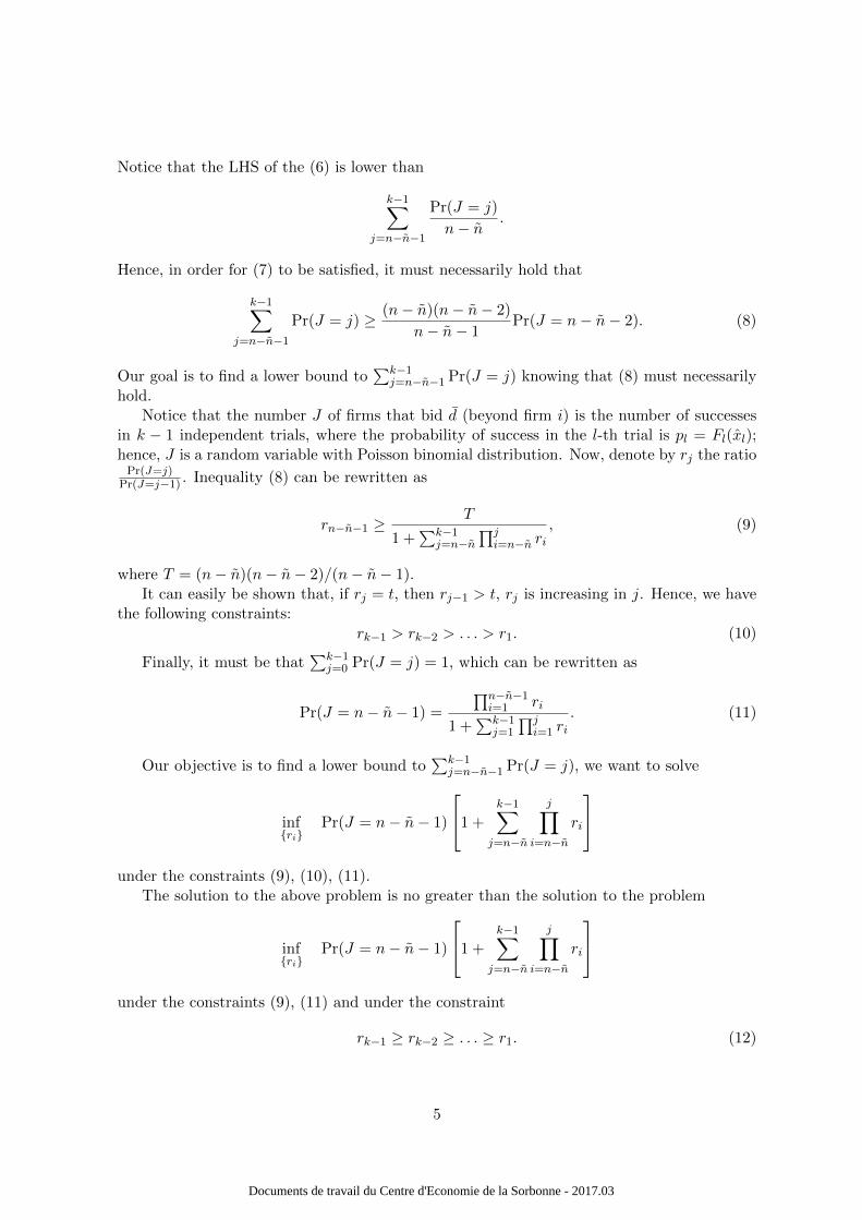
Notice that the LHS of the (6) is lower than

k−1∑j=n−n−1

Pr(J = j)

n− n.

Hence, in order for (7) to be satisfied, it must necessarily hold that

k−1∑j=n−n−1

Pr(J = j) ≥ (n− n)(n− n− 2)

n− n− 1Pr(J = n− n− 2). (8)

Our goal is to find a lower bound to∑k−1

j=n−n−1 Pr(J = j) knowing that (8) must necessarilyhold.

Notice that the number J of firms that bid d (beyond firm i) is the number of successesin k − 1 independent trials, where the probability of success in the l-th trial is pl = Fl(xl);hence, J is a random variable with Poisson binomial distribution. Now, denote by rj the ratio

Pr(J=j)Pr(J=j−1) . Inequality (8) can be rewritten as

rn−n−1 ≥T

1 +∑k−1

j=n−n∏j

i=n−n ri, (9)

where T = (n− n)(n− n− 2)/(n− n− 1).It can easily be shown that, if rj = t, then rj−1 > t, rj is increasing in j. Hence, we have

the following constraints:rk−1 > rk−2 > . . . > r1. (10)

Finally, it must be that∑k−1

j=0 Pr(J = j) = 1, which can be rewritten as

Pr(J = n− n− 1) =

∏n−n−1i=1 ri

1 +∑k−1

j=1

∏ji=1 ri

. (11)

Our objective is to find a lower bound to∑k−1

j=n−n−1 Pr(J = j), we want to solve

inf{ri}

Pr(J = n− n− 1)

1 +k−1∑

j=n−n

j∏i=n−n

ri

under the constraints (9), (10), (11).

The solution to the above problem is no greater than the solution to the problem

inf{ri}

Pr(J = n− n− 1)

1 +

k−1∑j=n−n

j∏i=n−n

ri

under the constraints (9), (11) and under the constraint

rk−1 ≥ rk−2 ≥ . . . ≥ r1. (12)

5


(We replaced (10) with a looser constraint). It’s easy to show, that, in the solution to theabove problem all constraints (9) and (12) are binding. Hence, the objective function isminimized at

r1 = r2 = . . . = rk − 1 = r, with

k−(n−n−1)∑j=1

rj = T,

and the minimum is∑k−1

j=n−n−1 rj/∑k−1

j=0 rj .

6


B Proof of Proposition 2

Proposition 2 can be easily obtained as a corollary of the following two lemmas that preciselycharacterize the asymptotic (optimal) behavior of level-k firms, k ≥ 1.

Lemma 3

(i) Consider the AB auction. Let δ(n)k (x) be the bidding strategy of a level-k firm, type x,

for k ≥ 1, when there are n firms and the other firms’ levels range from 0 to k− 1 (and

the proportion of level-j firms is pj/∑k−1

i=0 pi). Then, as n → ∞, δ(n)k (x) → A2k−1 for

all x, where:

– A20 = E[d0|A10 < d0 < d[90]];

– for j ≥ 1, A2j = (p0E[d0|A1j < d0 < d[90]] +∑j

i=1 piA2i−11[A2i−1>A1j ])/(p0 +∑j

i=1 pi1[A2i−1>A1j ]);

– A10 = E[d0|d[10] < d0 < d[90]];

– for j ≥ 1, A1j = (p0A10 +∑j

i=1 piA2i−1)/(∑j

i=0 pi);

– d[10] and d[90] are the 10-th and 90-th percentile of G0(d), G0(d[10]) = 0.1 andG0(d[90]) = 0.9.

(ii) Consider the ABL auction. Let δ(n)k (x) be the bidding strategy of a level-k firm, for

k ≥ 1, when there are n firms and the other firms’ levels range from 0 to k− 1 (and the

proportion of level-j firms is pj/∑k−1

i=0 pi). Then, as n→∞, δ(n)k (x)→ A3k−1 for all x,

where:

– for j ≥ 1, A3j = (A2j + d[10])/2;

– A20 = E[d0|A10 < d0 < d[90]];

– for j ≥ 1, A2j = (p0E[d0|A1j < d0 < d[90]] +∑j

i=1 piA3i−11[A3i−1>A1j ])/(p0 +∑j

i=1 pi1[A3i−1>A1j ]);

– A10 = E[d0|d[10] < d0 < d[90]];

– for j ≥ 1, A1j = (p0A10 +∑j

i=1 piA3i−1)/(∑j

i=0 pi);

– d[10] and d[90] are the 10-th and 90-th percentile of G0(d), G0(d[10]) = 0.1 andG0(d[90]) = 0.9.

Proof.

(i) Consider the AB auction. Let A1k−1 and A2k−1 be the value of A1 and A2 when firms’levels range from 0 to k−1 (with frequencies (p0/

∑k−1i=0 pi, . . . , pk−1/

∑k−1i=0 pi)), level-0

firms bid according to G0(d) and level-j firms, 0 < j ≤ k − 1 bid their best responseto their own beliefs. Consider a level-1 firm first. In order to choose her optimal bid, alevel-1 firm has to compute the probability distribution of the winning threshold A20,

which in turn depends on A10. Now, A10 =∑n−n

j=n+1 d(j)0 /(n − 2n), where d

(j)0 is the

j-th lowest bid by the level-0 firms. Let Yi, i = 1, . . . n be a sequence of i.i.d. randomvariables with distribution GY (y) = G0(y|d[10] < d0 < d[90]). The crucial thing to show

7


is that, when n → ∞, A10 converges almost surely to A10 = E[Y ]. To see this, notice

first that, by the strong law of large numbers,∑n

j=1 d(j)0 /n

a.s.−−→ E[d0], and, consequently,

d(n)0

a.s.−−→ d[10], d(n−n+1)0

a.s.−−→ d[90]. Now, let m1 = min{m ∈ 1, . . . , n : d(m)0 > d[10]} and

mn = max{m ∈ 1, . . . , n : d(m)0 < d[90]}. Notice that

∑m2j=m1

d(j)0 /(m2−m1+1) converges

almost surely to E[Y ] (because the random variables d(l)0 , with l ∈ [m1,m2] have the

same distributions as the Yi’s). Given this, in order to show that A10a.s.−−→ E[Y ], it is

sufficient to show that the difference A10−∑m2

j=m1d

(j)0 /(m2−m1 + 1) converges almost

surely to 0. Now, this difference can be written as

A10 −∑m2

j=m1d

(j)0

n− 2n+

∑m2j=m1

d(j)0

n− 2n−∑m2

j=m1d

(j)0

m2 −m1 + 1(13)

Notice that, since d0 ∈ [d, d] ⊆ [0, 1], the first two addends in (13) are certainly nogreater than

|m1 − n|+ |m2 − (n− n) + 1|n− 2n

,

and this term goes to 0 almost surely. The last two terms in (13) can be written as∑m2j=m1

d(j)0

m2 −m1 + 1

(m2 −m1 + 1

n− 2n− 1

).

Notice that the first fraction converges to E[Y ], and that (m2 −m1 + 1)/(n− 2n) goesto 1. Hence, expression (13) converges to 0 almost surely.

In a similar way, one can show that A20 converges almost surely to A20 = E[d0|A10 <d0 < d[90]]. Moreover, notice that, because G0(d) has full support, when n grows to

infinity, for all ε > 0, Pr(d0 ∈ (A20 − ε,A20)) → 1. Hence, as n increases, to get apositive chance of winning, a level-1 has to make a bid which is closer and closer to the

expected value (from her viewpoint) of the winning threshold A2, δ(n)1 (x) → A20, for

all x.

Consider now a level-2 firm. From her point of view, the winning threshold is A21,which, in turn, depends on A11. Reasoning in the same way as before, and given thatlevel-1 firms’ bids tend to A20, one show that A11 converges almost surely to A11 =(p0A10 + p1A20)/(p1 + p2), and A21 converges almost surely to A21 = (p0E[d0|A11 <d0 < d[90]] + p1A20)/(p0 + p1). As n increases, to get a positive chance of winning, alevel-2 has to make a bid which is closer and closer to the expected value (from her

viewpoint) of the winning threshold A2, δ(n)2 (x)→ A21, for all x.

Proceeding recursively, it is easy to show that, for all k ≥ 1, A1k converges almostsurely to A1k = (p0A10 +

∑ki=1 piA2i−1)/(

∑ki=0 pi), and A2k converges almost surely to

A2k =p0E[d0|A1k < d0 < d[90]] +

∑ki=1 piA2i−11[A2i−1>A1k]

p0 +∑k

i=1 pi1[A2i−1>A1k]

.

Hence, δ(n)k (x)→ A2k−1 for all x.

8


(ii) Apart from minor differences, the proof is the same for the ABL auction. Just one pointis worth mentioning: from the point of view of a level-k firm, when n grows to infinity,the interval from which the winning threshold is drawn, converges to [A3k−1, A2k−1].Now, since every number in this interval has the same probability of being extracted,

a level-k firm will bid closer and closer to the lowest value of this interval, δ(n)k (x) →

A3k−1.

Lemma 4

(i) In the AB auction, A2k−1 < A2k, for all k ≥ 1.

(ii) In the ABL auction: if A10 < (d[10] + A20)/2, then A2k−1 < A2k for all k ≥ 1; if

A10 > (d[10] + A20)/2, then A2k−1 > A2k for all k ≥ 1; if A10 = (d[10] + A20)/2, then

A2k−1 = A2k for all k ≥ 1.

Proof.

(i) Notice first that, by construction, for all k, A1k < A2k: in fact, A2k is a weightedaverage of numbers that are strictly greater than A2k. Second, for all k ≥ 1, A1k−1 <A1k < A2k−1: for k = 1, this is fairly obvious; for k > 1, notice that, since A1k−1 =(p0A10 +

∑k−1i=1 piA2i−1)/

∑k−1i=0 pi, we have that

k−1∑i=0

piA1k−1 = p0A10 +k−1∑i=1

piA2i−1.

Using this and substituting into the expression for A1k, we get

A1k =

∑k−1i=0 piA1k−1 + pkA2k−1∑k

i=0 pi.

Hence, A1k is a weighted average of A1k−1 and A2k−1, but since A1k−1 < A2k−1, itmust be A1k−1 < A1k < A2k−1.

We now show, by induction, that, if A2j−1 < A2j for all j ≤ k, then A2k < A2k+1. So,assume A2j−1 < A2j for all j ≤ k, k ≥ 1; let s = min j = 0, . . . , k − 1|A1k < A2j andlet t = min j = 0, . . . , k|A1k+1 < A2j . Notice that, necessarily, it must be s ≤ t; whens < t, we have

A2k =p0E[d0|A1k < d0 < d[90]] +

∑ki=s+1 piA2i−1

p0 +∑k

i=s+1 pi

=p0E[d0|A1k < d0 < d[90]] +

∑ti=s+1 piA2i−1 +

∑ki=t+1 piA2i−1

p0 +∑t

i=s+1 pi +∑k

i=t+1 pi.

Hence,

(p0 +t∑

i=s+1

pi +k∑

i=t+1

pi)A2k −t∑

i=s+1

piA2i−1 = p0E[d0|A1k < d0 < d[90]] +k∑

i=t+1

piA2i−1. (14)

9


Now, notice that, since A1k+1 > A1k, it must be

A2k+1 =p0E[d0|A1k+1 < d0 < d[90]] +

∑k+1i=t+1 piA2i−1

p0 +∑k+1

i=t+1 pi

>p0E[d0|A1k < d0 < d[90]] +

∑k+1i=t+1 piA2i−1

p0 +∑k+1

i=t+1 pi.

Using (14), the last inequality becomes

A2k+1 >(p0 +

∑ti=s+1 pi +

∑ki=t+1 pi)A2k −

∑ti=s+1 piA2i−1 + pk+1A2k

p0 +∑k+1

i=t+1 pi

=(p0 +

∑ki=t+1 pi + pk+1)A2k +

∑ti=s+1 pi(A2kA2i−1)

p0 +∑k+1

i=t+1 pi

=A2k +

∑ti=s+1 pi(A2kA2i−1)

p0 +∑k+1

i=t+1 pi

≥A2k.

When s = t, the whole derivation above goes through with the only difference that allterms involving

∑ti=s+1 are absent. To complete the proof, we have to show that A20 <

A21, which is fairly obvious, since A21 = (p0E[d0|A11 < d0 < d[90]] + p1A20)/(p0 + p1),

is a wighted average of A20 and a number (E[d0|A11 < d0 < d[90]]) strictly greater than

A20.

(ii) The proof for the ABL auction follows exactly the same line as the previous one withone caveat: if A10 < A30, we have that the sequence of A3k’s is strictly increasing;if, instead, A10 > A30, the sequence of A3k’s is strictly decreasing (in the proof, allinequalities are reversed); of course, it is in principle possible that A10 = A30, in whichcase the sequence of A3k’s is constant. (Typically, we expect A10 > A30: in fact, A30 isthe average between d[10] and A20, and the latter is no greater than d[90]; hence, if G0

is symmetric, A30 is necessarily below the mean of G0(d). To have A10 ≤ A30, G0(d)must be heavily skewed.)

The previous result immediately implies Proposition 2, that, for convenience, is reportedbelow.

Proposition 2. In the AB auction, in the limit, the (expected) distance of a firm’sbid from A2 is strictly decreasing in her level of sophistication. In the ABL auction, in thelimit, the (expected) distance of a firm’s bid from A3 is strictly decreasing in her level ofsophistication.42

Proof. Take the AB auction. If we denote by kmax the highest level of sophistication inthe population of firms, then: if kmax is finite, the expected value of A2, when n → ∞, issimply A2kmax+1; if not, the expected value of A2, when n→∞, is limk→∞A2k. In any case,A2k < E[A2], for all k. This, together with the fact that the sequence of A2k’s is strictly

42To be precise, this proposition holds only when A10 6= A30; when A10 6= A30, the (expected) distance ofa firm’s bid from A2 is constant in her level of sophistication.

10


increasing, implies that the distance between A2k (which is the optimal bid of a level-k + 1firm) and E[A2] is strictly decreasing in k.For the ABL auction, the proof is analogous.

11


C Numerical simulations

In this section, we present the results of some simulation exercises from a CH model of biddingbehavior in AB and ABL. The purpose of this exercise is twofold: on the one hand, it showsthat the main prediction of the CH model – the distance of a firm’s bid from A2 in AB,from A3 in ABL, is strictly decreasing in her level of sophistication – does not hold onlyasymptotically (as was proved in Proposition 2), but also for finite n; on the other hand, itprovides support to the additional empirical evidence presented in Subsection 5.4.

The simulations are run under the following assumptions and parametrization: we fixthe reserve price to 100 and assume that firms’ costs are private and independently andidentically distributed according to a uniform distribution on the interval [c = 50, c = 70],with increments of 0.2. We assume that firms’ levels of sophistication range from 0 to 243 andthat they are distributed according to a truncated Poisson with parameter λ.44 Level-0 firmsare assumed to draw their bids from a uniform distribution over the interval [0, 0.3]. Thisassumption is roughly consistent with our evidence (the minimum and maximum discountsobserved in our sample are 0 and 0.421 in AB and 0.016 and 0.317 in ABL) and ensuresthat level-0 firms will never play dominated strategies.45 Level-1 firms choose their bids tomaximize their expected payoffs under the belief that all other firms are level-0, while level-2firms choose their bids to maximize their expected payoffs under the belief that other firmsare a mixture of level-0 and level-1. Given the behavior of level-0, level-1 and level-2 firms, wecompute the expected value of A2 (for the AB auction) or A3 (for the ABL auction), and, foreach level, the expected value and the variance (in square brackets) of the distance betweentheir bids and A2 or A3. Since our objective is to check the consistency of the results of thesimulations with real data, we must allow for errors. Hence, the distance from A2 or A3 iscomputed supposing that level-1 and level-2 firms’ bids are subject to logistic errors: everybid is played with positive probability but the probability that a level-l firm (l = 1, 2) withcost c bids d is exp(ηΠl(d; c))/

∑d exp(ηΠl(d; c)), where Πl(d; c) is the expected payoff of a

level-l firm when her cost is c and she bids d, and where η denotes the error parameter (withη = 0 meaning random behavior and η →∞ meaning no errors). We also computed the trulyoptimal bid, , the bid that would maximize the expected payoff of a firm who has fully correctbeliefs about the behavior of other firms. Proposition 2 showed that, when n→∞, this trulyoptimal bid converges to A2 in AB, to A3 in ABL, but for finite n, it may be different. Hence,it is important to verify whether A2 and A3 are indeed good proxies for the optimal bid. Theresults of the simulations are reported in Tables C1-C6, for different values of the parameterof the distribution of levels (λ = 0.5, 1, 2), of the number of firms (n = 25, 50, 100) and of theparameter of the error distribution (η = 0.5, 1, 2).

43We consider only level-1 and level-2 firms because experimental evidence has shown that the majority ofsubjects performs no more than 2 levels of iteration (see, e.g., Crawford et al. 2013).

44Hence, the probability that a firm’s level of sophistication is l (l = 0, 1, 2) is equal to eλλl/l∑2i=0 e

λλi/i= λl/l

1+λ+λ2/2.

Hence, a higher λ means that firms are, on average, more sophisticated.45In this sense, level-0 firms have at least a minimum degree of rationality. Their random behavior could

be interpreted as the consequence of a total absence of any precise beliefs about the behavior of others. Theassumption that level-0 players do not play dominated strategies represents a small departure from the standardCH-literature. However, we believe that this represents a reasonable assumption in real world applications:all firms, also the most naive ones, should easily realize that it is not a good idea to offer a discount thatwould not allow it to cover the cost of realizing the work. In a similar vain, Goldfarb and Xiao (2011), in theirestimated CH-model of entry decisions by firms, endow level-0 firms with a minimum degree of rationality.

12


Table C1 – Simulation results for the AB auction with η = 0.5.

distance from A2 opt. distance from opt. bidn λ A2 level 0 level 1 level 2 bid level 0 level 1 level 2

0.5 20.3 8.5 [2.4] 5.2 [0.9] 4.2 [0.6] 20.4 8.5 [2.4] 5.3 [0.9] 4.3 [0.6]25 1 20.1 8.4 [2.4] 5.2 [0.9] 4.0 [0.5] 19.5 8.2 [2.3] 5.1 [0.9] 3.6 [0.4]

2 19.8 8.3 [2.3] 5.1 [0.9] 1.6 [0.1] 19.5 8.2 [2.3] 5.1 [0.9] 1.3 [0.1]

0.5 21.0 8.8 [2.6] 6.7 [1.5] 5.9 [1.2] 20.1-21.3 8.5 [2.4] 6.6 [1.4] 5.8 [1.1]50 1 20.7 8.6 [2.5] 6.6 [1.5] 5.9 [1.2] 20.4 8.5 [2.4] 6.6 [1.4] 5.8 [1.1]

2 20.6 8.6 [2.5] 6.6 [1.5] 2.6 [0.2] 20.4 8.5 [2.4] 6.6 [1.4] 2.4 [0.2]

0.5 21.0 8.8 [2.6] 7.7 [2.0] 7.1 [1.7] 20.4 8.5 [2.4] 7.5 [1.9] 7.0 [1.6]100 1 20.7 8.6 [2.5] 7.6 [1.93] 7.5 [1.88] 20.4 8.5 [2.4] 7.5 [1.9] 7.4 [1.8]

2 20.6 8.6 [2.5] 7.6 [1.9] 4.2 [0.6] 20.4 8.5 [2.4] 7.5 [1.9] 4.1 [0.5]

Table C2 – Simulation results for the AB auction with η = 1.


0.5 20.3 8.5 [2.4] 2.7 [0.2] 1.1 [0.0] 20.4 8.5 [2.4] 2.7 [0.2] 1.2 [0.0]25 1 20.1 8.4 [2.4] 2.6 [0.2] 1.5 [0.1] 19.5 8.2 [2.3] 2.6 [0.2] 0.9 [0.0]

2 19.8 8.3 [2.3] 2.6 [0.2] 0.6 [0.0] 19.5 8.2 [2.3] 2.6 [0.2] 0.3 [0.0]

0.5 21.0 8.8 [2.6] 4.2 [0.6] 2.1 [0.1] 20.1-21.3 8.5 [2.4] 4.1 [0.6] 2.4 [0.2]50 1 20.7 8.6 [2.5] 4.1 [0.6] 2.4 [0.2] 20.4 8.5 [2.4] 4.0 [0.5] 2.2 [0.2]

2 20.6 8.6 [2.5] 4.1 [0.6] 0.5 [0.0] 20.4 8.5 [2.4] 4.0 [0.5] 0.3 [0.0]

0.5 21.0 8.8 [2.6] 6.0 [1.2] 3.3 [0.4] 20.4 8.5 [2.4] 5.9 [1.2] 3.6 [0.4]100 1 20.7 8.6 [2.5] 6.0 [1.2] 4.7 [0.7] 20.4 8.5 [2.4] 5.9 [1.2] 4.5 [0.7]

2 20.6 8.6 [2.5] 6.0 [1.2] 0.9 [0.0] 20.4 8.5 [2.4] 5.9 [1.2] 0.7 [0.0]

Table C3 – Simulation results for the AB auction with η = 2.


0.5 20.3 8.5 [2.4] 1.1 [0.03] 0.2 [0.00] 20.4 8.5 [2.4] 1.1 [0.04] 0.3 [0.00]25 1 20.1 8.4 [2.4] 1.0 [0.03] 0.8 [0.02] 19.5 8.2 [2.3] 1.0 [0.03] 0.3 [0.00]

2 19.8 8.3 [2.3] 1.0 [0.03] 0.4 [0.00] 19.5 8.2 [2.3] 1.0 [0.03] 0.1 [0.00]

0.5 21.0 8.8 [2.6] 1.5 [0.08] 0.2 [0.00] 20.1-21.3 8.5 [2.4] 1.5 [0.07] 0.9 [0.03]50 1 20.7 8.6 [2.5] 1.4 [0.06] 0.5 [0.01] 20.4 8.5 [2.4] 1.4 [0.06] 0.3 [0.00]

2 20.6 8.6 [2.5] 1.4 [0.06] 0.3 [0.00] 20.4 8.5 [2.4] 1.4 [0.06] 0.0 [0.00]

0.5 21.0 8.8 [2.6] 2.8 [0.26] 0.5 [0.01] 20.4 8.5 [2.4] 2.8 [0.26] 1.0 [0.03]100 1 20.7 8.6 [2.5] 2.7 [0.25] 1.2 [0.05] 20.4 8.5 [2.4] 2.8 [0.26] 1.0 [0.03]

2 20.6 8.6 [2.5] 2.7 [0.25] 0.2 [0.00] 20.4 8.5 [2.4] 2.8 [0.26] 0.0 [0.00]

Looking at the results of these numerical simulations, we detect some regularities, thatwe summarize below.

(a) For all values of n, λ, and η, the optimal bid (, the bid that maximizes the expectedpayoff of a firm that has fully correct beliefs about the behavior of all other firms) isessentially unaffected by the private cost. In fact, of the 54 possible combinations ofparameters considered, there are only two cases in which the optimal bid is not constant

13


Table C4 – Simulation results for the ABL auction with η = 0.5.


0.5 13.5 7.7 [2.0] 5.6 [1.1] 4.5 [0.7] 15.0 7.6 [1.9] 5.0 [0.8] 4.1 [0.5]25 1 14.5 7.6 [1.9] 5.2 [0.9] 3.2 [0.4] 15.3 7.6 [1.9] 4.9 [0.8] 3.1 [0.3]

2 15.6 7.6 [1.9] 4.9 [0.8] 2.1 [0.1] 15.3 7.6 [1.9] 4.9 [0.8] 2.0 [0.1]

0.5 12.7 7.8 [2.0] 6.8 [1.6] 6.0 [1.2] 13.5 7.6 [1.9] 6.6 [1.4] 5.7 [1.1]50 1 13.5 7.7 [2.0] 6.6 [1.4] 5.0 [0.8] 15.0 7.6 [1.9] 6.3 [1.3] 4.7 [0.7]

2 15.3 7.6 [1.9] 6.2 [1.3] 3.3 [0.4] 15.3 7.6 [1.9] 6.2 [1.3] 3.3 [0.4]

0.5 12.7 7.8 [2.0] 7.3 [1.8] 6.9 [1.6] 15.6 7.6 [1.9] 6.9 [1.6] 6.6 [1.5]100 1 13.1 7.7 [2.0] 7.2 [1.7] 6.5 [1.4] 14.1 7.6 [1.9] 7.0 [1.6] 6.4 [1.4]

2 14.3 7.6 [1.9] 7.0 [1.6] 5.4 [1.0] 14.1 7.6 [1.9] 7.0 [1.6] 5.4 [1.0]

Table C5 – Simulation results for the ABL auction with η = 1.


0.5 13.5 7.7 [2.0] 4.2 [0.6] 2.3 [0.2] 15.0 7.6 [1.9] 3.1 [0.3] 1.5 [0.1]25 1 14.5 7.6 [1.9] 3.4 [0.4] 1.2 [0.0] 15.3 7.6 [1.9] 3.0 [0.3] 0.9 [0.0]

2 15.6 7.6 [1.9] 2.8 [0.3] 0.5 [0.0] 15.3 7.6 [1.9] 3.0 [0.3] 0.5 [0.0]

0.5 12.7 7.8 [2.0] 5.8 [1.1] 4.1 [0.5] 13.5 7.6 [1.9] 5.4 [1.0] 3.6 [0.4]50 1 13.5 7.7 [2.0] 5.4 [1.0] 2.6 [0.2] 15.0 7.6 [1.9] 4.8 [0.8] 2.0 [0.1]

2 15.3 7.6 [1.9] 4.8 [0.8] 0.9 [0.0] 15.3 7.6 [1.9] 4.8 [0.8] 0.9 [0.0]

0.5 12.7 7.8 [2.0] 6.8 [1.5] 6.0 [1.2] 15.6 7.6 [1.9] 6.2 [1.3] 5.5 [1.0]100 1 13.1 7.7 [2.0] 6.6 [1.4] 5.2 [0.9] 14.1 7.6 [1.9] 6.3 [1.3] 4.9 [0.8]

2 14.3 7.6 [1.9] 6.3 [1.3] 3.0 [0.3] 14.1 7.6 [1.9] 6.3 [1.3] 3.1 [0.3]

Table C6 – Simulation results for the ABL auction with η = 2.


0.5 13.5 7.7 [2.0] 3.3 [0.4] 1.7 [0.1] 15.0 7.6 [1.9] 1.9 [0.1] 0.5 [0.0]25 1 14.5 7.6 [1.9] 2.4 [0.2] 0.9 [0.0] 15.3 7.6 [1.9] 1.7 [0.1] 0.4 [0.0]

2 15.6 7.6 [1.9] 1.5 [0.1] 0.2 [0.0] 15.3 7.6 [1.9] 1.7 [0.1] 0.3 [0.0]

0.5 12.7 7.8 [2.0] 4.5 [0.7] 2.3 [0.2] 13.5 7.6 [1.9] 3.9 [0.5] 1.7 [0.1]50 1 13.5 7.7 [2.0] 3.9 [0.5] 1.6 [0.1] 15.0 7.6 [1.9] 2.9 [0.3] 0.6 [0.0]

2 15.3 7.6 [1.9] 2.8 [0.3] 0.3 [0.0] 15.3 7.6 [1.9] 2.7 [0.3] 0.3 [0.0]

0.5 12.7 7.8 [2.0] 5.7 [1.1] 4.2 [0.6] 15.6 7.6 [1.9] 4.6 [0.7] 3.4 [0.4]100 1 13.1 7.7 [2.0] 5.4 [1.0] 3.0 [0.3] 14.1 7.6 [1.9] 5.0 [0.8] 2.6 [0.2]

2 14.3 7.6 [1.9] 4.9 [0.8] 0.9 [0.0] 14.1 7.6 [1.9] 5.0 [0.8] 1.0 [0.0]

in the private cost: in AB, with η = 0.5, n = 50, λ = 0.5 and in AB, with η = 1, n = 50,λ = 0.5. Moreover, in these two cases, the range of the optimal bidding function ispretty narrow (about 1%). This confirms the intuition that, in these auctions, costs donot matter much for bidding.

(b) For all values of n, λ, and η, the optimal bid is extremely close to the expected value

14


of A2 in AB, of A3 in ABL. This supports the intuition that, in these auctions, A2 andA3 are good proxies for the optimal bid, even when n is finite.

(c) For all values of n, λ, and η, the distance of a firm’s bid from the expected value ofA2 in AB, of A3 in ABL, is decreasing in her level of sophistication. Hence, the maintheoretical prediction of the asymptotic CH model (Proposition 2) seem to hold alsowhen n is relatively small.

(d) For given n, λ, and η, level-1 and level-2 firms’ bids are, on average, lower in ABL thanin AB. This fact is consistent with the empirical evidence discussed in Subsection 5.4.

(e) In either auction, for all values of n, λ, and η, the variance of the distance from A2 orA3 is decreasing in the sophistication level of the firm. This fact is consistent with theempirical evidence discussed in Subsection 5.4.

(f) For given λ and η, the optimal bid and the expected value of A2 are increasing in nin AB, the optimal bid and the expected value of A3 are decreasing in n in ABL. Thisfact is consistent with the empirical evidence discussed in Subsection 5.4.

15


D Additional empirical evidence

This Section presents additional empirical evidence, both descriptive and inferential, recalledand commented in Sections 4 and 5 of the paper. In particular:

� Figures D1, D2 and D3 report descriptive evidence about the distribution of the sophis-tication index over time and by firm size;

� Table D1, columns (1) and (5), show that our main empirical result does not changewhen we amend our baseline model (2) including in the estimation those firms with asophistication index equal to 0 (replacing log(BidderSoph) with log(1 +BidderSoph));

� Table D1, columns (2) and (6), show that our main empirical result does not changewhen we amend our baseline model (2) adopting a log-linear specification instead of alog-log one;

� Table D1, columns (3) and (7), show that our main empirical result does not changewhen we amend our baseline model (2) adding the number of bidders as a controlvariable;

� Table D1, columns (4) and (8), show that our main empirical result does not changewhen we amend our baseline model (2) replacing auction controls with auction-fixedeffects;

� Table D2, columns (1)-(4), show, for the AB auctions, that our main empirical resultdoes not change when we adopt a two-step Heckman model to control for selection biasproblems;

� Table D2, columns (5)-(10), show, for the AB auctions, that our main empirical resultdoes not change when the sophistication index is category-specific: when a firm partic-ipates in auction j, only her performances in past auctions of the same format and ofthe same category of work as j are considered in the computation of her sophisticationlevel;

� Table D3, columns (1)-(4), show, for the AB sample, the estimation results when firm-and firm-year-fixed effects are not included in the model discussed in Subsection 4.5;

� Table D3, columns (5)-(8), show, for the AB sample, the estimation results when firm-year-fixed effects are replaced by firm-fixed effects in the model discussed in Subsection4.5;

� Table D4, columns (9)-(12), show, for the ABL sample, the estimation results of themodel discussed in Subsection 4.5;

� Table D4, columns (1)-(4), show, for the ABL sample, the estimation results when firm-and firm-year-fixed effects are not included in the model discussed in Subsection 4.5;

� Table D4, columns (5)-(8), show, for the ABL sample, the estimation results when firm-year-fixed effects are replaced by firm-fixed effects in the model discussed in Subsection4.5;

16


� Table D5 shows that our main empirical result does not change when we amend ourbaseline model (2) replacing firm- or firm-year-fixed effects with firm-semester or firm-category of work- or firm-category of work-semester- or firm-category of work-year-fixedeffects;

� Table D6 shows the estimation results of a model in which the dependent variable isthe level of bids;

� Table D7 shows the estimation results of quantile regression models in which the de-pendent variable is the level of bids;

� Table D8 shows that our main empirical result does not change when we control forpotential cartels in AB;

� Table D9 shows that our main empirical result does not change when we control forpotential cartels in ABL;

� Table D10 shows that the results of our IV regressions are unchanged when we focus onthe longer period 2004-2007;

� Table D11, columns (1) and (2), show that bids are, on average, lower in ABL than inAB;

� Table D11, column (3), shows that A2 in AB increases with the number of participatingfirms;

� Table D11, column (4), shows that A3 in ABL decreases with the number of participat-ing firms;

� Table D11, columns (5)-(10), show that the standard deviation of the average distancebetween bids and A2 [A3] in an AB [ABL] auction is decreasing in the average sophis-tication level of the firms participating in that auction.

17


Figure D1 – Distribution of the sophistication index in AB.

Figure D2 – Distribution of the sophistication index in ABL.

18


Figure D3 – Distribution of the sophistication index in AB by firm size.

19


Tab

leD

1–

Rob

ust

nes

sch

ecks

onth

eb

asel

ine

mod

elsp

ecifi

cati

on.

Dep

end

ent

vari

ab

le:

log|D

istance|

Au

ctio

nfo

rmat

AB

AB

AB

AB

AB

LA

BL

AB

LA

BL

(1)

(2)

(3)

(4)

(5)

(6)

(7)

(8)

log(1

+Bidder

Soph

)-0

.240***

-0.5

68***

(0.0

48)

(0.0

83)

Bidder

Soph

-0.0

20***

-0.1

13***

(0.0

03)

(0.0

21)

log(B

idder

Soph

)-0

.241***

-0.1

40***

-0.4

40***

-0.2

93***

(0.0

41)

(0.0

23)

(0.0

72)

(0.0

50)

Au

ctio

n/p

roje

ctco

ntr

ols

YE

SY

ES

YE

SN

OY

ES

YE

SY

ES

NO

Fir

mco

ntr

ols

NO

NO

NO

YE

SN

ON

ON

OY

ES

Fir

m-y

ear

FE

YE

SY

ES

YE

SN

OY

ES

YE

SY

ES

NO

Au

ctio

n-F

EN

ON

ON

OY

ES

NO

NO

NO

YE

SF

irm

-au

ctio

nco

ntr

ols

YE

SY

ES

YE

SY

ES

YE

SY

ES

YE

SY

ES

Ob

serv

ati

on

s8,9

65

8,9

65

8,5

73

8,9

24

1,5

91

1,5

91

1,2

66

1,5

01

R-s

qu

are

d0.3

61

0.3

61

0.3

56

0.3

79

0.5

24

0.5

16

0.5

06

0.3

61

OL

Ses

tim

ati

on

s.R

ob

ust

stan

dard

erro

rscl

ust

ered

at

firm

-lev

elin

pare

nth

eses

.In

fere

nce

:(*

**)

=p<

0.0

1,

(**)

=p<

0.0

5,

(*)

=p<

0.1

.Auction/project

controls

incl

ud

e:th

eau

ctio

n’s

rese

rve

pri

ce,

the

exp

ecte

dd

ura

tion

of

the

work

,d

um

my

vari

ab

les

for

the

typ

eof

work

,d

um

my

vari

ab

les

for

the

yea

rof

the

au

ctio

n,

an

d,

inco

lum

ns

(3)

an

d(7

),th

enu

mb

erof

bid

der

s.Firm

controls

incl

ud

e:d

um

my

vari

ab

les

for

firm

size

an

dfo

rth

ed

ista

nce

bet

wee

nth

efi

rman

dth

eC

A.Firm-auctioncontrols

incl

ud

e:a

du

mm

yvari

ab

lefo

rth

efi

rm’s

sub

contr

act

ing

posi

tion

(man

dato

ryor

op

tion

al)

,an

da

mea

sure

of

the

firm

’sb

ack

log.

20


Tab

leD

2–

AB

auct

ion

s:se

lect

ion

bia

sp

rob

lem

s(t

wo-

step

Hec

km

anm

odel

)an

dca

tego

ry-s

pec

ific

sop

his

tica

tion

ind

ex.

Dep

end

ent

vari

ab

le:

log|D

istance|

Pr.

Part

.lo

g|D

istance|

Pr.

Part

.lo

g|D

istance|

(1)

(2)

(3)

(4)

(5)

(6)

(7)

(8)

(9)

(10)

log(B

idder

Soph

)-0

.158***

-0.5

22***

0.2

28***

(0.0

26)

(0.0

38)

(0.0

21)

log(T

imeT

oBid

)0.0

34**

0.1

52***

(0.0

14)

(0.0

32)

log(B

idder

SophInCat)

-0.1

28***

-0.1

50***

-0.2

29***

(0.0

29)

(0.0

42)

(0.0

52)

log(1

+Bidder

SophInCat)

-0.1

79***

-0.2

54***

-0.3

88***

(0.0

32)

(0.0

51)

(0.0

63)

Au

ctio

n/p

roje

ctco

ntr

ols

YE

SY

ES

YE

SY

ES

YE

SY

ES

YE

SY

ES

YE

SY

ES

Fir

m-c

ontr

ols

YE

SY

ES

YE

SY

ES

YE

SY

ES

NO

NO

NO

NO

Fir

m-F

EN

ON

ON

ON

ON

ON

OY

ES

YE

SN

ON

OF

irm

-yea

rF

EN

ON

ON

ON

ON

ON

ON

ON

OY

ES

YE

SF

irm

-au

ctio

nco

ntr

ols

NO

NO

NO

NO

YE

SY

ES

YE

SY

ES

YE

SY

ES

Ob

serv

ati

on

s3,8

77

13,5

17

13,5

17

13,5

17

3,6

58

3,9

82

3,6

58

3,9

10

3,5

56

3,7

27

R-s

qu

are

d0.1

90

0.0

47

0.1

90

0.1

99

0.2

67

0.2

77

0.3

72

0.3

78

OL

Ses

tim

ati

on

s.R

ob

ust

stan

dard

erro

rscl

ust

ered

at

firm

-lev

elin

pare

nth

eses

.In

fere

nce

:(*

**)

=p<

0.0

1,

(**)

=p<

0.0

5,

(*)

=p<

0.1

.Auction/project

controls

incl

ud

e:th

eau

ctio

n’s

rese

rve

pri

ce,

the

exp

ecte

dd

ura

tion

of

the

work

,d

um

my

vari

ab

les

for

the

yea

rof

the

au

ctio

n.

Firm

controls

incl

ud

e:d

um

my

vari

ab

les

for

firm

’ssi

zean

dfo

rth

ed

ista

nce

bet

wee

nth

efi

rman

dth

eC

A.Firm-auction

controls

incl

ud

e:a

du

mm

yvari

able

for

the

firm

’ssu

bco

ntr

act

ing

posi

tion

(man

dato

ryor

op

tion

al)

,an

da

mea

sure

of

the

firm

’sb

ack

log.

Th

ean

aly

sis

focu

ses

on

AB

au

ctio

ns

for

road

work

sb

ecau

seth

eyre

pre

sent

the

larg

est

share

of

pro

ject

sin

ou

rd

ata

(87

au

ctio

ns)

.O

LS

regre

ssio

nin

colu

mn

(1)

show

sth

eco

effici

ent

ofBidder

Soph

esti

mate

don

the

sub

sam

ple

of

road

work

s.T

he

pote

nti

al

mark

etfo

rro

ad

work

sis

defi

ned

as

those

firm

sth

at,

acc

ord

ing

toou

rd

ata

set,

bid

at

least

on

cefo

rro

ad

work

sin

agiv

enyea

r.A

san

exogen

ou

sin

stru

men

tth

at

isre

late

dto

the

pro

bab

ilit

yof

firm

s’p

art

icip

ati

on

bu

th

as

an

infl

uen

ceon

lyon

the

cost

of

part

icip

ati

on

,w

eu

seTim

eToBid

,w

hic

his

the

len

gth

of

tim

eb

etw

een

the

date

wh

enth

ep

roje

ctis

ad

ver

tise

dan

dw

hen

the

bid

lett

ing

occ

urs

(th

isin

stru

men

tis

als

ou

sed

by

Gil

an

dM

ari

on

2013,

an

dM

ore

tti

an

dV

alb

on

esi

2015).

Th

ehyp

oth

esis

isth

at

the

lon

ger

the

tim

eb

etw

een

the

beg

inn

ing

of

pro

ject

’sp

ub

lici

tyan

dth

ed

ead

lin

efo

rb

id’s

sub

mis

sion

,th

elo

wer

the

cost

born

eby

firm

sto

pre

pare

thei

rbid

s.O

ur

data

show

that

ther

eis

vari

ab

ilit

yin

term

sof

au

ctio

ns’

ad

ver

tise

lead

tim

e,w

ith

an

aver

age

of

28.6

days

(an

da

stan

dard

dev

iati

on

of

11.4

days)

.In

colu

mn

s(3

)an

d(4

),th

ese

con

dan

dfi

rst

stage

of

atw

o-s

tep

Hec

km

an

sele

ctio

nm

od

elare

rep

ort

ed.

21


Tab

leD

3–

Lea

rnin

gd

yn

amic

s:fu

rth

erre

sult

sfo

rA

Bau

ctio

ns.

Dep

end

ent

vari

ab

lelo

g|D

istance|

Au

ctio

nfo

rmat

AB

(1)

(2)

(3)

(4)

(5)

(6)

(7)

(8)

log(P

astPart)

-0.1

39***

-0.1

20***

-0.1

13***

-0.2

12***

-0.2

25***

-0.2

43***

(0.0

24)

(0.0

21)

(0.0

23)

(0.0

41)

(0.0

42)

(0.0

43)

log(1

+PastPer

f)

-2.8

25***

-2.8

11***

0.9

17*

0.8

60

(0.2

29)

(0.2

30)

(0.5

41)

(0.5

48)

log(1

+PastW

ins)

-0.0

32

-0.0

27

0.1

95**

0.1

92**

(0.0

48)

(0.0

56)

(0.0

80)

(0.0

76)

log(B

idder

Soph

)-0

.166***

-0.1

86***

(0.0

25)

(0.0

39)

Au

ctio

n/p

roje

ctco

ntr

ols

YE

SY

ES

YE

SY

ES

YE

SY

ES

YE

SY

ES

Fir

mco

ntr

ols

YE

SY

ES

YE

SY

ES

NO

NO

NO

NO

Fir

m-F

EN

ON

ON

ON

OY

ES

YE

SY

ES

YE

SF

irm

-au

ctio

nco

ntr

ols

YE

SY

ES

YE

SY

ES

YE

SY

ES

YE

SY

ES

Ob

serv

ati

on

s8,9

27

8,9

27

8,9

27

8,9

27

8,8

38

8,8

38

8,8

38

8,8

38

R-s

qu

are

d0.1

88

0.2

04

0.2

04

0.1

92

0.2

67

0.2

67

0.2

68

0.2

67

OL

Ses

tim

ati

on

s.R

ob

ust

stan

dard

erro

rscl

ust

ered

at

firm

-lev

elin

pare

nth

eses

.In

fere

nce

:(*

**)

=p<

0.0

1,

(**)

=p<

0.0

5,

(*)

=p<

0.1

.Auction/project

controls

incl

ud

e:th

eau

ctio

n’s

rese

rve

pri

ce,

the

exp

ecte

dd

ura

tion

of

the

work

,d

um

my

vari

ab

les

for

the

typ

eof

work

,d

um

my

vari

ab

les

for

the

yea

rof

the

au

ctio

n.Firm

controls

incl

ud

e:d

um

my

vari

ab

les

for

the

size

of

the

firm

,an

dth

ed

ista

nce

bet

wee

nth

efi

rman

dth

eC


incl

ud

e:a

du

mm

yvari

ab

lefo

rth

efi

rm’s

sub

contr

act

ing

posi

tion

(man

dato

ryor

op

tion

al)

,an

da

mea

sure

of

the

firm

’sb

ack

log.

22


Tab

leD

4–

Lea

rnin

gd

yn

amic

s:re

sult

sfo

rA

BL

auct

ion

s.

Dep

enden

tvari

ab

lelo

g|D

istance|

Au

ctio

nfo

rmat

AB

L(1

)(2

)(3

)(4

)(5

)(6

)(7

)(8

)(9

)(1

0)

(11)

(12)

log(P

astPart)

-0.2

72***

-0.2

60***

-0.2

71***

-0.5

58***

-0.5

28***

-0.5

38***

-0.6

01***

-0.5

64***

-0.5

75***

(0.0

58)

(0.0

49)

(0.0

50)

(0.0

73)

(0.0

77)

(0.0

77)

(0.0

75)

(0.0

79)

(0.0

79)

log(1

+PastPer

f)

-2.8

73***

-2.9

12***

-0.7

35

-0.7

52

-0.8

70

-0.8

73

(0.3

26)

(0.3

27)

(0.6

90)

(0.6

88)

(0.7

07)

(0.7

03)

log(1

+PastW

ins)

0.3

50**

0.3

23**

0.3

53

0.3

47

0.3

74

0.3

58

(0.1

50)

(0.1

53)

(0.2

46)

(0.2

41)

(0.2

85)

(0.2

75)

log(B

idder

Soph

)-0

.395***

-0.4

77***

-0.5

17***

(0.0

43)

(0.0

64)

(0.0

67)

Au

ctio

n/p

roje

ctco

ntr

ols

YE

SY

ES

YE

SY

ES

YE

SY

ES

YE

SY

ES

Fir

mco

ntr

ols

YE

SY

ES

YE

SY

ES

NO

NO

NO

NO

NO

NO

NO

NO

Fir

m-F

EN

ON

ON

ON

OY

ES

YE

SY

ES

YE

SN

ON

ON

ON

OF

irm

-yea

r-F

EN

ON

ON

ON

ON

ON

ON

ON

OY

ES

YE

SY

ES

YE

SF

irm

-au

ctio

nco

ntr

ols

YE

SY

ES

YE

SY

ES

YE

SY

ES

YE

SY

ES

YE

SY

ES

YE

SY

ES

Ob

serv

ati

on

s1,5

01

1,5

01

1,5

01

1,5

01

1,4

10

1,4

10

1,4

10

1,4

10

1,2

66

1,2

66

1,2

66

1,2

66

R-s

qu

are

d0.2

44

0.2

96

0.2

98

0.2

80

0.4

59

0.4

59

0.4

60

0.4

60

0.4

50

0.4

50

0.4

51

0.4

51

OL

Ses

tim

ati

on

s.R

ob

ust

stan

dard

erro

rscl

ust

ered

at

firm

-lev

elin

pare

nth

eses

.In

fere

nce

:(*

**)

=p<

0.0

1,

(**)

=p<

0.0

5,

(*)

=p<

0.1

.Auction/project

controls

incl

ud

e:th

eau

ctio

n’s

rese

rve

pri

ce,

the

exp

ecte

dd

ura

tion

of

the

work

,d

um

my

vari

ab

les

for

the

typ

eof

work

,d

um

my

vari

ab

les

for

the

yea

rof

the

au

ctio

n.Firm

controls

incl

ud

e:d

um

my

vari

ab

les

for

the

size

of

the

firm

,an

dth

ed

ista

nce

bet

wee

nth

efi

rman

dth

eC


incl

ud

e:a

du

mm

yvari

ab

lefo

rth

efi

rm’s

sub

contr

act

ing

posi

tion

(man

dato

ryor

op

tion

al)

,and

am

easu

reof

the

firm

’sb

ack

log.

23


Tab

leD

5–

Fu

rth

erre

sult

s:fi

rm-c

ateg

ory

ofw

ork-fi

xed

effec

tsan

dfi

rm-s

emes

ter

fixed

effec

ts.

Dep

enden

tvari

ab

lelo

g|D

istance|

Au

ctio

nfo

rmat

AB

AB

AB

LA

BL

AB

LA

BL

(1)

(2)

(3)

(4)

(5)

(6)

log(B

idder

Soph

)-0

.166***

-0.1

24**

-0.0

89

-0.4

76***

-0.5

07***

0.1

32

(0.0

40)

(0.0

52)

(0.1

17)

(0.0

76)

(0.1

02)

(0.1

64)

Au

ctio

n/p

roje

ctco

ntr

ols

YE

SY

ES

YE

SY

ES

YE

SY

ES

Fir

m-s

emes

ter-

FE

NO

NO

YE

SN

ON

ON

OF

irm

-cate

gory

of

work

-FE

YE

SN

ON

OY

ES

NO

NO

Fir

m-c

ate

gory

of

work

-sem

este

r-F

EN

OY

ES

NO

NO

NO

YE

SF

irm

-cate

gory

of

work

-yea

r-F

EN

ON

ON

ON

OY

ES

NO

Fir

m-a

uct

ion

contr

ols

YE

SY

ES

YE

SY

ES

YE

SY

ES

Ob

serv

ati

on

s8,6

42

7,4

63

1,1

54

1,2

87

1,0

53

838

R-s

qu

are

d0.3

03

0.4

78

0.5

80

0.5

28

0.5

84

0.6

91

OL

Ses

tim

ati

on

s.R

ob

ust

stan

dard

erro

rscl

ust

ered

at

firm

-lev

elin

pare

nth

eses

.In

fere

nce

:(*

**)

=p<

0.0

1,

(**)

=p<

0.0

5,

(*)

=p<

0.1

.Auction/project

controls

incl

ud

e:th

eau

ctio

n’s

rese

rve

pri

ce,

the

exp

ecte

dd

ura

tion

of

the

work

,du

mm

yvari

ab

les

for

the

typ

eof

work

,d

um

my

vari

ab

les

for

the

yea

rof

the

auct

ion

.Firm-auction

controls

incl

ud

e:a

du

mm

yvari

ab

lefo

rth

efi

rm’s

sub

contr

act

ing

posi

tion

(man

dato

ryor

op

tion

al)

,an

da

mea

sure

of

the

firm

’sb

ack

log.

24


Tab

leD

6–

Sop

his

tica

tion

and

bid

leve

ls:

over

all

sam

ple

.

Dep

end

ent

vari

ab

lelo

g(D

iscount)

Discount

log(D

iscount)

Discount

log(D

iscount)

Discount

log(D

iscount)

Discount

Au

ctio

nfo

rmat

AB

AB

AB

AB

AB

LA

BL

AB

LA

BL

(1)

(2)

(3)

(4)

(5)

(6)

(7)

(8)

log(B

idder

Soph

)0.0

06

0.0

83

-0.0

16

-0.2

47*

-0.0

14

-0.3

67

-0.0

15

-0.3

90

(0.0

10)

(0.1

17)

(0.0

13)

(0.1

42)

(0.0

22)

(0.2

39)

(0.0

24)

(0.2

60)

Au

ctio

n/p

roje

ctco

ntr

ols

YE

SY

ES

YE

SY

ES

YE

SY

ES

YE

SY

ES

Fir

m-F

EY

ES

YE

SN

ON

OY

ES

YE

SN

ON

OF

irm

-yea

r-F

EN

ON

OY

ES

YE

SN

ON

OY

ES

YE

SF

irm

-au

ctio

nco

ntr

ols

YE

SY

ES

YE

SY

ES

YE

SY

ES

YE

SY

ES

Ob

serv

ati

on

s8,8

38

8,8

38

8,5

73

8,5

73

1,4

10

1,4

10

1,2

66

1,2

66

R-s

qu

are

d0.3

48

0.5

30

0.4

22

0.5

90

0.5

25

0.6

78

0.5

83

0.7

15

OL

Ses

tim

ati

on

s.R

ob

ust

stan

dard

erro

rscl

ust

ered

at

firm

-lev

elin

pare

nth

eses

.In

fere

nce

:(*

**)

=p<

0.0

1,

(**)

=p<

0.0

5,

(*)

=p<

0.1

.Auction/project

controls

incl

ud

e:th

eau

ctio

n’s

rese

rve

pri

ce,

the

exp

ecte

dd

ura

tion

of

the

work

,du

mm

yvari

ab

les

for

the

typ

eof

work

,d

um

my

vari

ab

les

for

the

yea

rof

the

auct

ion

.Firm-auction

controls

incl

ud

e:a

du

mm

yvari

ab

lefo

rth

efi

rm’s

sub

contr

act

ing

posi

tion

(man

dato

ryor

op

tion

al)

,an

da

mea

sure

of

the

firm

’sb

ack

log.

25


Tab

leD

7–

Sop

his

tica

tion

and

bid

leve

ls:

qu

anti

lere

gres

sion

s.

Qu

anti

le(th

)5

10

20

30

40

50

60

70

80

90

95

Au

ctio

nfo

rmat

AB

Dep

end

ent

log(D

iscount)

log(B

idder

Soph

)0.0

40***

0.0

28***

0.0

11***

0.0

07***

0.0

04***

0.0

02*

0.0

01

0.0

01

-0.0

00

-0.0

03***

-0.0

08***

(0.0

08)

(0.0

06)

(0.0

03)

(0.0

02)

(0.0

01)

(0.0

01)

(0.0

01)

(0.0

01)

(0.0

01)

(0.0

01)

(0.0

02)

Dep

end

ent

Discount

log(B

idder

Soph

)0.6

35***

0.4

21***

0.1

93***

0.1

25***

0.0

74***

0.0

36**

0.0

23

0.0

13

-0.0

04

-0.0

61***

-0.1

66***

(0.1

10)

(0.0

90)

(0.0

47)

(0.0

27)

(0.0

23)

(0.0

18)

(0.0

17)

(0.0

15)

(0.0

16)

(0.0

17)

(0.0

37)

Ob

serv

ati

on

s8,9

27

8,9

27

8,9

27

8,9

27

8,9

27

8,9

27

8,9

27

8,9

27

8,9

27

8,9

27

8,9

27

Au

ctio

nfo

rmat

AB

LD

epen

den

tlo

g(D

iscount)

log(B

idder

Soph

)0.0

65***

0.0

54***

0.0

26***

0.0

13***

0.0

04

0.0

00

-0.0

08

-0.0

22***

-0.0

51***

-0.0

81***

-0.0

91***

(0.0

18)

(0.0

16)

(0.0

08)

(0.0

05)

(0.0

04)

(0.0

04)

(0.0

05)

(0.0

08)

(0.0

13)

(0.0

05)

(0.0

11)

Dep

end

ent

Discount

log(B

idder

Soph

)0.5

99***

0.5

37***

0.2

95***

0.1

53***

0.0

53

0.0

02

-0.1

01

-0.2

97***

-0.7

64***

-1.3

30***

-1.6

15***

(0.1

60)

(0.1

44)

(0.0

99)

(0.0

58)

(0.0

47)

(0.0

47)

(0.0

69)

(0.1

10)

(0.1

88)

(0.0

92)

(0.1

61)

Ob

serv

ati

on

s1,5

01

1,5

01

1,5

01

1,5

01

1,5

01

1,5

01

1,5

01

1,5

01

1,5

01

1,5

01

1,5

01

Au

ctio

n/p

roje

ctco

ntr

ols

YE

SY

ES

YE

SY

ES

YE

SY

ES

YE

SY

ES

YE

SY

ES

YE

SF

irm

contr

ols

YE

SY

ES

YE

SY

ES

YE

SY

ES

YE

SY

ES

YE

SY

ES

YE

SF

irm

-au

ctio

nco

ntr

ols

YE

SY

ES

YE

SY

ES

YE

SY

ES

YE

SY

ES

YE

SY

ES

YE

S

Rob

ust

stan

dard

erro

rscl

ust

ered

at

firm

-lev

elin

pare

nth

eses

.In

fere

nce

:(*

**)

=p<

0.0

1,

(**)

=p<

0.0

5,

(*)

=p<

0.1

.Auction/project

controls

incl

ud

e:th

eau

ctio

n’s

rese

rve

pri

ce,

the

exp

ecte

dd

ura

tion

of

the

work

,du

mm

yvari

ab

les

for

the

typ

eof

work

,d

um

my

vari

ab

les

for

the

yea

rof

the

au

ctio

n.Firm

controls

incl

ud

e:d

um

my

vari

ab

les

for

the

size

of

the

firm

,an

dth

ed

ista

nce

bet

wee

nth

efi

rman

dth

eC

A.Firm-auction

controls

incl

ud

e:a

du

mm

yvari

ab

lefo

rth

efi

rm’s

sub

contr

act

ing

posi

tion

(man

dato

ryor

op

tion

al)

,an

da

mea

sure

of

the

firm

’sb

ack

log.

26


Tab

leD

8–

Con

trollin

gfo

rp

oten

tial

cart

els

inA

Bau

ctio

ns.

Dep

end

ent

log|D

istance|

Au

ctio

nfo

rmat

AB

(1)

(2)

(3)

(4)

(5)

(6)

(7)

(8)

log(B

idder

Soph

)-0

.163***

-0.1

63***

-0.1

96***

-0.1

93***

-0.2

83***

-0.2

83***

-0.1

53***

-0.1

99***

(0.0

23)

(0.0

23)

(0.0

37)

(0.0

37)

(0.0

44)

(0.0

44)

(0.0

31)

(0.0

54)

log(1

+Groupmem

bers)

-0.1

69***

0.0

31

-0.2

29***

-0.1

82

-0.2

37***

-0.2

40*

(0.0

32)

(0.0

68)

(0.0

45)

(0.1

14)

(0.0

54)

(0.1

37)

log(1

+Groupmem

bers)

xShareG

roupmem

bers

-0.4

16***

-0.7

29***

-0.4

65

(0.1

20)

(0.2

52)

(0.2

83)

ShareG

roupmem

bers

0.1

53

1.2

60**

0.8

97

(0.0

95)

(0.5

46)

(0.6

74)

Au

ctio

n/p

roje

ctco

ntr

ols

YE

SY

ES

YE

SY

ES

YE

SY

ES

YE

SY

ES

Fir

mco

ntr

ols

YE

SY

ES

NO

NO

NO

NO

YE

SN

OF

irm

-FE

NO

NO

YE

SY

ES

NO

NO

NO

YE

SF

irm

-yea

r-F

EN

ON

ON

ON

OY

ES

YE

SN

ON

OF

irm

-au

ctio

nco

ntr

ols

YE

SY

ES

YE

SY

ES

YE

SY

ES

YE

SY

ES

Ob

serv

ati

on

s8,0

37

8,0

37

7,9

45

7,9

45

7,9

45

7,9

45

3,8

61

3,8

28

R-s

qu

are

d0.2

02

0.2

03

0.2

66

0.2

67

0.3

68

0.3

69

0.1

81

0.3

02

OL

Ses

tim

ati

on

s.R

ob

ust

stan

dard

erro

rscl

ust

ered

at

firm

-lev

elin

pare

nth

eses

.In

fere

nce

:(*

**)

=p<

0.0

1,

(**)

=p<

0.0

5,

(*)

=p<

0.1

.Auction/project

controls

incl

ud

e:th

eau

ctio

n’s

rese

rve

pri

ce,

the

exp

ecte

dd

ura

tion

of

the

work

,du

mm

yvari

ab

les

for

the

typ

eof

work

,d

um

my

vari

ab

les

for

the

yea

rof

the

au

ctio

n.Firm

controls

incl

ud

e:d

um

my

vari

ab

les

for

the

size

of

the

firm

,an

dth

ed

ista

nce

bet

wee

nth

efi

rman

dth

eC

A.Firm-auction

controls

incl

ud

e:a

du

mm

yvari

ab

lefo

rth

efi

rm’s

sub

contr

act

ing

posi

tion

(man

dato

ryor

op

tion

al)

,an

da

mea

sure

of

the

firm

’sb

ack

log.

27


Tab

leD

9–

Con

trol

lin

gfo

rp

oten

tial

cart

els

inA

BL

auct

ion

s.

Dep

end

ent

log|D

istance|

Au

ctio

nfo

rmat

AB

L(1

)(2

)(3

)(4

)(5

)(6

)(7

)(8

)(9

)lo

g(B

idder

Soph

)-0

.369***

-0.3

56***

-0.4

30***

-0.4

28***

-0.4

90***

-0.4

85***

-0.2

70***

-0.3

65***

-0.4

21***

(0.0

49)

(0.0

51)

(0.0

67)

(0.0

67)

(0.0

79)

(0.0

80)

(0.0

71)

(0.1

04)

(0.1

25)

log(1

+Groupmem

bers)

0.0

29

0.3

01**

-0.1

41

0.1

57

-0.1

70

0.1

05

(0.0

56)

(0.1

20)

(0.1

24)

(0.4

44)

(0.1

50)

(0.6

03)

log(1

+Groupmem

bers)

xShareG

roupmem

bers

-0.5

28**

-0.4

58

-0.4

66

(0.2

43)

(0.4

53)

(0.5

49)

ShareG

roupmem

bers

0.3

15

0.1

00

0.1

57

(0.2

63)

(1.3

85)

(1.8

61)

Au

ctio

n/p

roje

ctco

ntr

ols

YE

SY

ES

YE

SY

ES

YE

SY

ES

YE

SY

ES

YE

SF

irm

contr

ols

YE

SY

ES

NO

NO

NO

NO

YE

SN

ON

OF

irm

-FE

NO

NO

YE

SY

ES

NO

NO

NO

YE

SN

OF

irm

-yea

r-F

EN

ON

ON

ON

OY

ES

YE

SN

ON

OY

ES

Fir

m-a

uct

ion

contr

ols

YE

SY

ES

YE

SY

ES

YE

SY

ES

YE

SY

ES

YE

SO

bse

rvati

on

s1,3

16

1,3

16

1,3

16

1,3

16

1,3

12

1,3

12

578

578

578

R-s

qu

are

d0.2

64

0.2

68

0.4

59

0.4

61

0.5

69

0.5

70

0.2

40

0.5

98

0.7

16

OL

Ses

tim

ati

on

s.R

ob

ust

stan

dard

erro

rscl

ust

ered

at

firm

-lev

elin

pare

nth

eses

.In

fere

nce

:(*

**)

=p<

0.0

1,

(**)

=p<

0.0

5,

(*)

=p<

0.1

.Auction/project

controls

incl

ud

e:th

eau

ctio

n’s

rese

rve

pri

ce,

the

exp

ecte

dd

ura

tion

of

the

work

,du

mm

yvari

ab

les

for

the

typ

eof

work

,d

um

my

vari

ab

les

for

the

yea

rof

the

au

ctio

n.Firm

controls

incl

ud

e:d

um

my

vari

ab

les

for

the

size

of

the

firm

,an

dth

ed

ista

nce

bet

wee

nth

efi

rman

dth

eC

A.Firm-auction

controls

incl

ud

e:a

du

mm

yvari

ab

lefo

rth

efi

rm’s

sub

contr

act

ing

posi

tion

(man

dato

ryor

op

tion

al)

,an

da

mea

sure

of

the

firm

’sb

ack

log.

28


Tab

leD

10

–F

urt

her

2SL

Ses

tim

atio

ns

Dep

end

ent

vari

ab

lelo

g(B

idder

Soph

)(B

idder

Soph

)|D

istance||D

istance|

Au

ctio

nfo

rmat

AB

+A

BL

AB

+A

BL

AB

+A

BL

AB

+A

BL

1’s

tage

1’s

tage

2’s

tage

2’s

tage

(1)

(2)

(3)

(4)

log(B

idder

Soph

)-0

.162***

-0.1

82***

(0.0

24)

(0.0

29)

ABL

-0.5

35***

-0.6

12***

(0.1

65)

(0.1

54)

log(B

idder

Soph

00−

03)

0.7

05***

(0.0

41)

ABL∗

log(B

idder

Soph

00−

03)

-0.5

85***

-0.5

82***

(0.0

50)

(0.0

47)

Au

ctio

n/p

roje

ctco

ntr

ols

YE

SY

ES

YE

SY

ES

Fir

mco

ntr

ols

YE

SN

OY

ES

NO

Fir

m-fi

xed

effec

tsN

OY

ES

NO

YE

SF

irm

-au

ctio

nco

ntr

ols

YE

SY

ES

YE

SY

ES

Ob

serv

ati

on

s2,9

54

2,9

54

2,9

54

2,9

54

R-s

qu

are

d0.8

31

0.8

15

0.0

60

0.0

62

Han

sen

-Jte

st0.7

22

0.4

90

Rob

ust

stan

dard

erro

rscl

ust

ered

at

firm

-lev

elin

pare

nth

eses

.In

fere

nce

:(*

**)

=p<

0.0

1,

(**)

=p<

0.0

5,

(*)

=p<

0.1

.Auction/project

controls

incl

ud

e:th

eau

ctio

n’s

rese

rve

pri

ce,

the

exp

ecte

dd

ura

tion

of

the

work

,d

um

my

vari

ab

les

for

the

typ

eof

work

.Firm

controls

incl

ud

e:d

um

my

vari

ab

les

for

the

size

ofth

efi

rm,an

dth

ed

ista

nce

bet

wee

nth

efi

rman

dth

eC

A.Firm-

auction

controls

incl

ud

e:a

du

mm

yvari

ab

lefo

rth

efi

rm’s

sub

contr

act

ing

posi

tion

(man

dato

ryor

op

tion

al)

,an

da

mea

sure

of

the

firm

’sb

ack

log.

29


Tab

leD

11

–A

dd

itio

nal

emp

iric

aled

vid

ence

.

Dep

end

ent

vari

ab

le:

Normalized

Normalized

A2

A3

Auction

Auction

Firm

Firm

Firm

Firm

Discount

Discount

St.Dev

.St.Dev

.St.Dev

.St.Dev

.St.Dev

.St.Dev

.A

uct

ion

form

at

AB

+A

BL

AB

+A

BL

AB

AB

LA

BA

BL

AB

AB

LA

BA

BL

(1)

(2)

(3)

(4)

(5)

(6)

(7)

(8)

(9)

(10)

ABL

-0.3

66***

-0.4

20***

(0.0

22)

(0.0

18)

log(N

o.P

articipants

)0.4

63**

-0.7

12**

(0.2

21)

(0.2

84)

log(M

eanBidder

Soph

)-0

.304*

-0.7

34**

(0.1

61)

(0.1

65)

log(R

ollin

gM

eanBidder

Soph

)-0

.292***

-0.6

04***

-0.6

44***

-0.9

43***

(0.0

47)

(0.1

68)

(0.1

13)

(0.2

25)

Au

ctio

n/p

roje

ctco

ntr

ols

YE

SY

ES

YE

SY

ES

YE

SY

ES

NO

NO

NO

NO

Fir

mco

ntr

ols

YE

SN

ON

ON

ON

ON

OY

ES

YE

SN

ON

OF

irm

-fixed

effec

tsN

OY

ES

NO

NO

NO

NO

NO

NO

YE

SY

ES

Fir

m-a

uct

ion

contr

ols

YE

SY

ES

NO

NO

NO

NO

NO

NO

NO

NO

Ob

serv

ati

on

s10,4

28

9,6

47

232

28

228

26

7,2

73

656

7,2

73

656

R-s

qu

are

d0.1

88

0.2

48

0.8

48

0.9

93

0.2

43

0.7

61

0.2

12

0.2

25

0.3

80

0.6

01

Inco

lum

ns

(1)-

(2)

an

d(7

)-(1

0):

OL

Ses

tim

ati

on

san

dro

bu

stst

an

dard

erro

rscl

ust

ered

at

firm

-lev

elin

pare

nth

eses

.In

colu

mn

s(3

)-(6

),an

IRL

Ses

tim

ato

ris

use

dto

acc

ou

nt

for

the

infl

uen

ceof

ou

tlie

rs(g

iven

the

small

sam

ple

s).

Infe

ren

ce:

(***)

=p<

0.0

1,

(**)

=p<

0.0

5,

(*)

=p<

0.1

.In

colu

mn

s(1

)an

d(2

),th

ed

epen

den

tvari

ab

leis

the

(min

-max

resc

ale

d)

dis

cou

nt

off

ered

by

firm

s.ABL

isa

du

mm

yvari

ab

lew

hic

hta

kes

valu

e1

(0)

ifth

eau

ctio

nis

AB

L(A

B).

Th

ou

gh

not

rep

ort

ed,

the

sop

his

tica

tion

ind

exis

incl

ud

edam

on

gth

eco

vari

ate

s.In

colu

mn

s(3

)an

d(4

)th

ed

epen

den

tvari

ab

leis

the

(au

ctio

n-s

pec

ific)

refe

ren

cep

oin

t.In

colu

mn

s(5

)an

d(6

)th

ed

epen

den

tvari

ab

leSDauction

isth

est

an

dard

dev

iati

on

of

the

(ab

solu

tevalu

eof

the

stan

dard

ized

)d

ista

nce

of

bid

sfr

om

the

refe

ren

cep

oin

t.In

colu

mn

s(7

)an

d(1

2)

the

dep

end

ent

vari

ab

leRollin

gSDfirm

isth

ero

llin

gst

an

dard

dev

iati

on

of

the

(ab

solu

tevalu

eof

the

stan

dard

ized

)d

ista

nce

of

bid

sfr

om

the

refe

ren

cep

oin

tin

the

last

five

au

ctio

ns.

Mea

nBidder

Soph

isth

eaver

age

of

the

sop

his

tica

tion

ind

exacr

oss

firm

sin

the

au

ctio

n.

Rollin

gM

eanBidder

Soph

isth

ero

llin

gaver

age

of

the

sop

his

tica

tion

ind

exof

the

firm

inth

ela

stfi

ve

au

ctio

ns.

Auction/project

controls

incl

ud

e:th

eau

ctio

n’s

rese

rve

pri

ce,

the

exp

ecte

dd

ura

tion

of

the

work

,d

um

my

vari

ab

les

for

the

typ

eof

work

,d

um

my

vari

ab

les

for

the

yea

rof

the

au

ctio

n.Firm

controls

incl

ud

e:du

mm

yvari

ab

les

for

the

size

of

the

firm

,an

dth

ed

ista

nce

bet

wee

nth

efi

rman

dth

eC

A.Firm-auction

controls

incl

ud

e:a

du

mm

yvari

ab

lefo

rth

efi

rm’s

sub

contr

act

ing

posi

tion

(man

dato

ryor

op

tion

al)

,an

da

mea

sure

of

the

firm

’sb

ack

log.

Inco

lum

ns

(7)-

(10)

tim

ed

um

mie

sta

kin

gth

evalu

e1

for

the

mea

nyea

rof

the

bid

der

s’la

stfi

ve

au

ctio

ns

are

incl

ud

ed.

30
