Embed Size (px)
Citation preview

SONOELECTROCHEMICAL (20 kHz) PRODUCTION
OF HYDROGEN FROM AQUEOUS SOLUTIONS
BY
DANIEL SYMES
Thesis submitted in accordance with the requirements of
The University of Birmingham for the degree of
MASTER OF RESEARCH
School of Chemical Engineering
College of Engineering and Physical Sciences
The University of Birmingham
February 2011

University of Birmingham Research Archive
e-theses repository This unpublished thesis/dissertation is copyright of the author and/or third parties. The intellectual property rights of the author or third parties in respect of this work are as defined by The Copyright Designs and Patents Act 1988 or as modified by any successor legislation. Any use made of information contained in this thesis/dissertation must be in accordance with that legislation and must be properly acknowledged. Further distribution or reproduction in any format is prohibited without the permission of the copyright holder.

ACKNOWLEDGEMENTS
I am whole heartily thankful to my supervisor Dr Bruno G. Pollet, whose encouragement, supervision,
and support from the preliminary to concluding level enabled me to develop and understanding of
the subject.
I would also like to express my gratitude to the EPSRC for providing the funding for this research, and
thank my family and girlfriend for their love and support throughout.
Finally I offer my regards to Matthew Lepesant whose assistance in the laboratory was of great aid to
me, blessings to Professor Kevin Kendall, Dr Waldemar Bujalski, Dr Aman Dhir, Oliver Curnick, James
Courtney, Tony Meadowcroft and fellow researchers at the PEM Fuel Cell Research Group and the
Centre for Hydrogen and Fuel Cell Research at the University of Birmingham, who supported me in
any respect during the completion of the project.

ABSTRACT
There are various methods of producing Hydrogen. These include electrolysis, which this work is
based upon, and steam reforming; currently the most commercially viable method.
The research herein investigates methods of producing ‘green’ Hydrogen more efficiently by using
ultrasound (20 kHz) combined to electrolysis. Previous studies have shown that ultrasound enhances
mass-transfer of electro-active species from the bulk solution to the electrode surface in any
electrolytic system and mechanically removes gas bubbles on the electrode surface.
This work takes this previous research further by quantifying actual hydrogen gas output. The
hydrogen evolution reaction was then directly compared with that calculated using the Ideal Gas
Equation to quantify the efficiency of the electrolysis system.
It was observed that ultrasound lowers the anodic and cathodic overpotentials due to gas removal at
the electrode surface induced by cavitation and increased mass-transfer. However, it was found that
ultrasound did not increase the rate of Hydrogen production. During experimentation it was seen
that the force exhibited on the electrodes by ultrasonic waves limited bubble evolution on the
electrode surface.
Issues associated with the ultrasonic reactor geometry and the ultrasonic transducer size are also
discussed as potential reasons for this result.

CONTENTS
1. INTRODUCTION & LITERATURE SURVEY ............................................................................................. 1
1.1 Global Warming and Carbon Dioxide ............................................................................................ 1
1.2 Hydrogen as an Energy Carrier ...................................................................................................... 4
1.2.1 What is Hydrogen? ................................................................................................................. 4
1.2.2 Methods of Hydrogen Production ......................................................................................... 6
1.2.3 Fuel Cell Technology ............................................................................................................. 13
1.3 Principles of Electrochemistry ..................................................................................................... 17
Method 1: Decomposition Voltage ............................................................................................... 19
Method 2: Discharge Potential ..................................................................................................... 20
1.4 Electrolysis ................................................................................................................................... 22
1.5 Sonoelectrochemistry ................................................................................................................. 25
1.6 Sonoelectrochemical Production of Hydrogen ........................................................................... 30
2. EXPERIMENTAL METHOD .................................................................................................................. 33
2.1 Equipment & Parameters ............................................................................................................ 37
3. RESULTS AND DISCUSSION ................................................................................................................ 38
3.1 Preliminary Experiments ............................................................................................................. 38
3.1.1 Current Voltage Curves ........................................................................................................ 38
3.1.2 Overpotential Determination ............................................................................................... 43
3.2 Custom Glassware Experiments .................................................................................................. 46
3.2.1 Current-Voltage Curves ........................................................................................................ 46
3.2.2 Hydrogen Evolution Rate ..................................................................................................... 49
3.2.3 Hydrogen Efficiency Data ..................................................................................................... 53
3.2.4 Energy Efficiency Data .......................................................................................................... 56
3.2.5 Ultrasonic Power Determination ......................................................................................... 56
3.3 Erosion of the Electrodes ............................................................................................................ 57
3.4 Experiments with Industrial Electrolysers ................................................................................... 58

3.4.1 Introduction.......................................................................................................................... 58
3.4.2 Data Analysis ........................................................................................................................ 60
4. CONCLUSIONS ................................................................................................................................... 63
4.1 Comparison for Industrial Electrolyser and Sonoelectrochemical Cell ....................................... 66
5. FUTURE WORK .................................................................................................................................. 69
5.1 Electrolytes .................................................................................................................................. 69
5.2 Electrode Parameters .................................................................................................................. 70
5.3 Electrolyte Temperature ............................................................................................................. 70
5.4 Ultrasonic Parameters ................................................................................................................. 71
6. REFERENCES ...................................................................................................................................... 72
7. APPENDICES ...................................................................................................................................... 77
7.1 Appendix I - Data Tables .............................................................................................................. 77
7.1.1 Preliminary Experiments ...................................................................................................... 77
7.1.2 Custom Glassware Experiments ........................................................................................... 83
7.2 Appendix II - Graphs .................................................................................................................. 143
7.2.1 Preliminary Experiments .................................................................................................... 143
7.2.2 Custom Glassware Experiments ......................................................................................... 146
7.3 Appendix III – Decomposition Potential Calculations ............................................................... 155
7.4 Appendix IV - Ultrasound Power Data Tables ........................................................................... 158
7.5 Appendix V - Health & Safety .................................................................................................... 159
7.6 Appendix VI – Conferences Attended & Posters Presented ..................................................... 163

TABLE OF FIGURES
Figure 1: Greenhouse Effect Diagram. Source: United Nation Environment Programme...................... 1
Figure 2: Flammability Range of H2 when compared to other fuels. Source: Hydrogen-FC Ltd ............. 5
Figure 3: A summary of the current technologies available to produce Hydrogen [40] ...................... 12
Figure 4: Diagram of a PEMFC [43] ....................................................................................................... 14
Figure 5: Decomposition Voltage Calculation Demonstration Graph ................................................... 20
Figure 6: Schematic of Ultrasonic Phenomena [69] .............................................................................. 27
Figure 7: Custom Designed Glassware & Experimental Setup .............................................................. 33
Figure 8: Experimental Setup for Preliminary Experiments .................................................................. 34
Figure 9: Decomposition Curves for NaOH solution ............................................................................. 38
Figure 10: Decomposition Curves for NaCl solution ............................................................................. 39
Figure 11: Decomposition Curves for H2SO4 solution ............................................................................ 40
Figure 12: Current Voltage Comparison Graph for all three electrolytes ............................................. 41
Figure 13: Current Enhancement for NaOH solution ............................................................................ 46
Figure 14: Current Enhancement for NaCl solution .............................................................................. 47
Figure 15: Current Enhancement for H2SO4 solution ............................................................................ 48
Figure 16: Hydrogen Production Enhancement for NaOH solution ...................................................... 49
Figure 17: Hydrogen Production Enhancement for NaCl solution ........................................................ 50
Figure 18: Hydrogen Production Enhancement for H2SO4 solution ...................................................... 51
Figure 19: Hydrogen Output Efficiency Enhancement for NaOH solution ............................................ 53
Figure 20: Hydrogen Output Efficiency Enhancement for NaCl solution .............................................. 54
Figure 21: Hydrogen Output Efficiency Enhancement for H2SO4 solution ............................................ 55
Figure 22: Image of Experimental Setup ............................................................................................... 58
Figure 23: Image showing small leak on side tank ................................................................................ 59
Figure 24: Decomposition Curves for KOH solution .............................................................................. 60
Figure 25: HHO Production for KOH solution ........................................................................................ 62
Figure 26: Diagram defining the Sonication Distance ........................................................................... 66
Figure 27: Table of Voltage Current Data for NaOH ............................................................................. 77
Figure 28: Table of Voltage Current Data for NaCl ............................................................................... 78
Figure 29: Table of Voltage Current Data for H2SO4 ............................................................................. 79
Figure 30: Table of Voltage Current Data for NaOH Sonicated ............................................................. 80
Figure 31: Table of Voltage Current Data for NaCl Sonicated ............................................................... 81
Figure 32: Table of Voltage Current Data for H2SO4 Sonicated ........................................................... 82
Figure 33: Data for 0.1M NaOH Silent ................................................................................................... 83
Figure 34: Data for 0.2M NaOH Silent ................................................................................................... 84
Figure 35: Data for 0.3M NaOH Silent ................................................................................................... 85
Figure 36: Data for 0.4M NaOH Silent ................................................................................................... 86
Figure 37: Data for 0.5M NaOH Silent ................................................................................................... 87
Figure 38: Data for 1.0M NaOH Silent ................................................................................................... 88
Figure 39: Data of NaOH Efficiency of H2 production ........................................................................... 89
Figure 40: Data for 0.1M NaCl Silent ..................................................................................................... 90

Figure 41: Data for 0.2M NaCl Silent ..................................................................................................... 91
Figure 42: Data for 0.3M NaCl Silent ..................................................................................................... 92
Figure 43: Data for 0.4M NaCl Silent ..................................................................................................... 93
Figure 44: Data for 0.5M NaCl Silent ..................................................................................................... 94
Figure 45: Data for 1.0M NaCl Silent ..................................................................................................... 95
Figure 46: Data of NaCl Efficiency of H2 production ............................................................................. 96
Figure 47: Data for 0.1M H2SO4 Silent ................................................................................................... 97
Figure 48: Data for 0.2M H2SO4 Silent ................................................................................................... 98
Figure 49: Data for 0.3M H2SO4 Silent ................................................................................................... 99
Figure 50: Data for 0.4M H2SO4 Silent ................................................................................................. 100
Figure 51: Data for 0.5M H2SO4 Silent ................................................................................................. 101
Figure 52: Data for 1.0M H2SO4 Silent ................................................................................................. 102
Figure 53: Data of H2SO4 Efficiency of H2 production ......................................................................... 103
Figure 54: Data for 0.1M NaOH Sonicated .......................................................................................... 104
Figure 55: Data for 0.2M NaOH Sonicated .......................................................................................... 105
Figure 56: Data for 0.3M NaOH Sonicated .......................................................................................... 106
Figure 57: Data for 0.4M NaOH Sonicated .......................................................................................... 107
Figure 58: Data for 0.5M NaOH Sonicated .......................................................................................... 108
Figure 59: Data for 1.0M NaOH Sonicated .......................................................................................... 109
Figure 60: Data of NaOH Efficiency of H2 production ......................................................................... 110
Figure 61: Data for 0.1M NaCl Sonicated ............................................................................................ 111
Figure 62: Data for 0.2M NaCl Sonicated ............................................................................................ 112
Figure 63: Data for 0.3M NaCl Sonicated ............................................................................................ 113
Figure 64: Data for 0.4M NaCl Sonicated ............................................................................................ 114
Figure 65: Data for 0.5M NaCl Sonicated ............................................................................................ 115
Figure 66: Data for 1.0M NaCl Sonicated ............................................................................................ 116
Figure 67: Data of NaCl Efficiency of H2 production ........................................................................... 117
Figure 68: Data for 0.1M H2SO4 Sonicated .......................................................................................... 118
Figure 69: Data for 0.2M H2SO4 Sonicated .......................................................................................... 119
Figure 70: Data for 0.3M H2SO4 Sonicated .......................................................................................... 120
Figure 71: Data for 0.4M H2SO4 Sonicated .......................................................................................... 121
Figure 72: Data for 0.5M H2SO4 Sonicated .......................................................................................... 122
Figure 73: Data for 1.0M H2SO4 Sonicated .......................................................................................... 123
Figure 74: Data of H2SO4 Efficiency of H2 production ......................................................................... 124
Figure 75: Data for 0.1M NaOH Ultrasound Enhancement ................................................................ 125
Figure 76: Data for 0.2M NaOH Ultrasound Enhancement ................................................................ 126
Figure 77: Data for 0.3M NaOH Ultrasound Enhancement ................................................................ 127
Figure 78: Data for 0.4M NaOH Ultrasound Enhancement ................................................................ 128
Figure 79: Data for 0.5M NaOH Ultrasound Enhancement ................................................................ 129
Figure 80: Data for 1.0M NaOH Ultrasound Enhancement ................................................................ 130
Figure 81: Data for 0.1M NaCl Ultrasound Enhancement .................................................................. 131
Figure 82: Data for 0.2M NaCl Ultrasound Enhancement .................................................................. 132
Figure 83: Data for 0.3M NaCl Ultrasound Enhancement .................................................................. 133

Figure 84: Data for 0.4M NaCl Ultrasound Enhancement .................................................................. 134
Figure 85: Data for 0.5M NaCl Ultrasound Enhancement .................................................................. 135
Figure 86: Data for 1.0M NaCl Ultrasound Enhancement .................................................................. 136
Figure 87: Data for 0.1M H2SO4 Ultrasound Enhancement ................................................................ 137
Figure 88: Data for 0.2M H2SO4 Ultrasound Enhancement ................................................................ 138
Figure 89: Data for 0.3M H2SO4 Ultrasound Enhancement ................................................................ 139
Figure 90: Data for 0.4M H2SO4 Ultrasound Enhancement ................................................................ 140
Figure 91: Data for 0.5M H2SO4 Ultrasound Enhancement ................................................................ 141
Figure 92: Data for 1.0M H2SO4 Ultrasound Enhancement ................................................................ 142
Figure 93: Current Voltage Graph for Silent NaOH solution ............................................................... 143
Figure 94: Current Voltage Graph for Silent NaCl solution ................................................................. 143
Figure 95: Current Voltage Graph for Silent H2SO4 solution ............................................................... 144
Figure 96: Current Voltage Graph for Sonicated NaOH solution ........................................................ 144
Figure 97: Current Voltage Graph for Sonicated NaCl solution .......................................................... 145
Figure 98: Current Voltage Graph for Sonicated H2SO4 solution ........................................................ 145
Figure 99: Current Voltage Graph for Silent NaOH solution ............................................................... 146
Figure 100: Current Voltage Graph for Silent NaCl solution ............................................................... 146
Figure 101: Current Voltage Graph for Silent H2SO4 solution ............................................................. 147
Figure 102: Current Voltage Graph for Sonicated NaOH solution ...................................................... 147
Figure 103: Current Voltage Graph for Sonicated NaCl solution ........................................................ 148
Figure 104: Current Voltage Graph for Sonicated H2SO4 solution ...................................................... 148
Figure 105: Hydrogen Production Graph for Silent NaOH solution .................................................... 149
Figure 106: Hydrogen Production Graph for Silent NaCl solution ...................................................... 149
Figure 107: Hydrogen Production Graph for Silent H2SO4 solution .................................................... 150
Figure 108: Hydrogen Production Graph for Sonicated NaOH solution ............................................. 150
Figure 109: Hydrogen Production Graph for Sonicated NaCl solution ............................................... 151
Figure 110: Hydrogen Production Graph for Sonicated H2SO4 solution ............................................. 151
Figure 111: Hydrogen Production Efficiency Graph for Silent NaOH solution .................................... 152
Figure 112: Hydrogen Production Efficiency Graph for Silent NaCl solution ...................................... 152
Figure 113: Hydrogen Production Efficiency Graph for Silent H2SO4 solution .................................... 153
Figure 114: Hydrogen Production Efficiency Graph for Sonicated NaOH solution ............................. 153
Figure 115: Hydrogen Production Efficiency Graph for Sonicated NaCl solution ............................... 154
Figure 116: Hydrogen Production Efficiency Graph for Sonicated H2SO4 solution ............................. 154
Figure 117: Temperature variance table for each electrolyte at varying ultrasonic powers .............. 158
Figure 118: dT/dt gradients calculated for each electrolyte ............................................................... 158
Figure 119: Ultrasound Power Table ................................................................................................... 158

TABLE OF TABLES
Table 1: Comparison of Fuel Cell Technologies [48] ............................................................................. 15
Table 2: Preliminary Experimental Electrolyte Masses ......................................................................... 35
Table 3: Custom Glassware Experimental Electrolyte Masses .............................................................. 35
Table 4: Table of Decomposition Voltages ............................................................................................ 43
Table 5: Table of Overpotentials ........................................................................................................... 43
Table 6: Table of Average Overpotentials ............................................................................................. 44
Table 7: Chemical Properties for each electrolyte solution [94] ........................................................... 56
Table 8: Ultrasonic Power Density Table .............................................................................................. 57
Table 9: Decomposition Voltages for Industrial Electrolyser ................................................................ 61

1
1. INTRODUCTION & LITERATURE SURVEY
Global energy demand and security as well as increasing world population are leading to an
inevitable shortage of fossil fuels which is the primary resource of our energy requirement. Fossil
fuels are made up of hydrocarbons, and as their availability becomes increasingly limited, other
energy sources will need to be found, in other words, research into new sources of energy is urgently
required [1].
1.1 Global Warming and Carbon Dioxide
Carbon dioxide (CO2), one of the main contributors to global warming, was first discovered in 1753 by
Joseph Black whilst he was at the University of Edinburgh completing his medical studies. It was not
for another 50 years until Jean-Baptiste Fourier suggested that an atmospheric effect kept the planet
warmer than it should be. This
occurred in 1827 whereby Fourier
used the analogy of a
‘greenhouse’ to describe this
atmospheric effect [2].
Then in 1896 a direct link between
CO2 and global warming was
found, where Arrhenius proposed
that CO2 emissions from burning
coal would enhance the planet’s greenhouse effect and lead to global warming. Since the industrial
revolution, which began in the early 18th century, the amount of CO2 in the atmosphere has
increased by 35%. It is reported that the current level of CO2 in the atmosphere is higher than it was
650,000 years ago [3].
Figure 1: Greenhouse Effect Diagram. Source: United Nation Environment Programme

2
CO2 absorbs and emits waves in the infrared (IR) spectrum and it is known as a greenhouse gas
(GHG). Other GHGs include NOx, CO, O3, SOx and H2O. As the Earth is heated by the Sun, the
greenhouse gases in the troposphere absorb the reflected solar radiation and emit it back to Earth.
The amount of solar radiation absorbed is directly proportional to the amount of greenhouse gases in
the troposphere. As the level of CO2 in the atmosphere increases, more solar radiation becomes
trapped thus increasing the temperature of the planet leading to global warming [4] (Figure 1 [5]).
Fossil fuels when combusted to produce energy create CO2 and other GHGs as by-products. The CO2
concentration in the Earth’s atmosphere has been steadily increasing for the last 100 years [6], due
to the rise in quantities of fossil fuels being burnt together with rapid deforestation. Deforestation
results in a reduction of photosynthesis i.e. decreasing the removal carbon dioxide from the
atmosphere and its replacement with oxygen in turn causing CO2 levels in the atmosphere to rise [7].
The rising population of our planet (currently ca. 6 billion and expected to rise over 9 billion by 2050)
is also leading to higher emissions. Indeed, this increase in population will cause a growing demand
for food, livestock and energy, all of which will result in higher CO2 emissions [8].
Another cause of increasing CO2 concentration in the atmosphere is due to the depletion of the
ozone (O3) layer in the upper atmosphere. O3 prevents harmful UV rays from the Sun reaching the
surface of the planet and if there was no ozone, no life would exist!
Both of these phenomena have resulted in an increase in average global temperature of around 2-
4oC over the last 100 years. In that period, it is reported that the burning of fossil fuels has produced
about three quarters of the increase in CO2 levels and the remaining is due to land use changes e.g.
deforestation (e.g. Amazon forest) [7].
Throughout the history of our planet, the Earth has always been changing, sometimes through
natural causes. More recently the term ‘climate change’ has been used to describe changes in our
climate since the early 20th century. The changes in climate we have seen recently along with the

3
changes predicted over the next 100 years are not solely due to natural causes, but are thought to be
caused by human activities (anthropogenic activities) [2].
Governments started to realise the need for action by raising awareness of the alarming global issue.
In 1979, the world held its first climate conference. The conference called upon governments “to
foresee and prevent potential man-made changes in climate”. In 1988, the United Nations (UN) set
up the Intergovernmental Panel on Climate Change (IPCC) to analyse and report on scientific findings
[2].
The first Earth Summit was held in Rio de Janeiro in 1992, where the United Nations Framework
Convention on Climate Change (UNFCCC) was signed by 154 nations. It was agreed to prevent
“dangerous” warming from GHGs and set voluntary targets for reducing their emissions. The UNFCCC
agreed voluntary targets in 1992 and the Kyoto Protocol was the first international treaty to set
legally binding GHG emissions cuts for industrialised nations. The agreement was signed by 178
countries in 1997 and came into force in 2005 [2].
However, a potential solution to this problem presented above is the use of Hydrogen as an energy
carrier/vector, and this is hereby discussed.

4
1.2 Hydrogen as an Energy Carrier
1.2.1 What is Hydrogen?
Hydrogen was first discovered in 1766 by Henry Cavendish through the reactions of zinc (Zn) and
hydrochloric acid (HCl), which led to the discovery that water is made up of Hydrogen (H2) and
Oxygen (O2) [9]. This was the only method of Hydrogen production (and in fact of ‘green’ Hydrogen)
for over a hundred years until British scientists William Nicholson and Sir Anthony Carlisle discovered
that applying an electrical current to water produces Hydrogen and Oxygen gases in 1880 [10]. This
was later termed ' Water Electrolysis'.
In 1970, the Electrochemist John Bockris coined the term 'Hydrogen economy'[11, 12] and at the first
World Hydrogen Conference in 1976 the idea of a Hydrogen economy was first discussed, identifying
Hydrogen energy as a clean energy carrier for the future. It was concluded that a large proportion of
energy supplied by Hydrogen, could be made from sources that have no net GHG emissions. The
concept of a Hydrogen economy came about due to the limitations of fossil fuel supply and concerns
about global warming [12].
Hydrogen is currently commercially produced by steam reforming (SR), which unfortunately releases
GHGs, most notably carbon monoxide (CO) and CO2 into the atmosphere. This results in the
Hydrogen energy not being carbon neutral and therefore not meeting the objectives proposed in
1976 at the World Hydrogen Conference. Currently, it is more cost effective to produce Hydrogen
from fossil fuels; therefore producers do not invest in the Hydrogen produced from renewable
sources.
Many academics, some politicians and industrialists believe that the only realistic method to produce
‘green’ Hydrogen without creating any GHGs is through the use of renewable energy sources. These
include solar (photovoltaic and photocatalysis), wind, tidal, geothermal and hydroelectric energy
sources. Energy can be produced by these sources indefinitely as the primary sources of the energy

5
(the Sun for solar power, heat produced from the Earth for geothermal energy) will always exist
whilst there is life on Earth. It is important to note that Hydrogen is an energy carrier, not a primary
energy source [13]. Another source capable of producing Hydrogen is nuclear energy (via Electrolysis
– see later). This method for producing Hydrogen has a lot of sceptics, but there is a great public
concern over the disposal of the radioactive waste created from the process.
Hydrogen is predicted to be one of the future fuels for the automotive, buildings and portable
electronic sectors [14]. In each of these sectors, the
Hydrogen energy is converted to electricity and heat
by the fuel cell with water being the only by-product.
Hydrogen is an extremely flammable substance and
must be handled with care, with a wide range of
flammability limits and a low ignition energy [15]
(Figure 2 [16]). This means that Hydrogen must be
stored in a heat free environment with no source of
ignition in the vicinity. These properties also create a
high risk of fire and/or explosion [15]. When Hydrogen
ignites, it burns with a colourless flame, which in itself is a hazard since it is difficult to detect.
Another potential hazard of Hydrogen is if it leaks from a high pressure source (350 or 700 bar)
Hydrogen self-heats itself, creating the risk of fires and/or explosions [17].
Currently vehicles running on petrol/diesel are known to have low energy efficiencies (<40%), but the
lack of alternative fuels and an infrastructure means that there is no direct competition for
petrol/diesel. Gasoline used in Internal Combustion Engines (ICEs) is found to have an energy
efficiency of approximately 35%, whereas Hydrogen has an efficiency of approximately 41%.
Therefore, Hydrogen supply chains would release significantly less CO2 than the production of
Figure 2: Flammability Range of H2 when compared to other fuels. Source: Hydrogen-FC Ltd

6
gasoline for Hybrid Electric Vehicles. Emissions created during production could be reduced by
Carbon Capture and Sequestration (CCS) at the site of production [18].
The use of Hydrogen in a Hydrogen Fuel Cell or a Hydrogen ICE, requires storage that has inherent
and high volumetric efficiency. Metal Hydrides (M-H) offer alternatives to storing Hydrogen in gas
and liquid form and are typically 0.5-3% weight H2. They store Hydrogen in what is essentially a solid
form and offer the potential of high safety, volume efficiency, low pressure containment (<10 bar)
and operating conditions at ambient temperatures [19].
The introduction of alternative fuels will require significant, long-term investments for setting up and
expanding infrastructures[20]. This is especially true in the case of a Hydrogen economy based on
renewable resources. Today’s decisions therefore should be oriented towards robust options with
stable prospects even under changing future framework conditions. Long-term scenarios are one tool
for finding robust options because they allow outlining future developments of energy systems in
relation to a variety of framework conditions and policy settings.
These scenarios refer to the total energy system so as to provide a complete balance of energy
consumption and GHG emissions, and to take shifts between different sectors into account. A
scenario analysis is required because depending on how fast the share of HFC vehicles expands, the
impacts on final energy consumption, the energy demand for Hydrogen, and the resulting GHG
emissions will differ [18].
1.2.2 Methods of Hydrogen Production
Currently 50 million tonnes of Hydrogen are produced globally every year. It is predicted that the
production will rise by 10% year-on-year over the next decade. Steam reforming (SR) is the most
widely used method to produce Hydrogen and currently accounts for 95-96% of global Hydrogen
production where as electrolysis only contributes 4-5%.

7
1.2.2.1 Hydrogen Production by Electrolysis
Water electrolysis involves passing an electrical current through water, to split the water molecules
into Hydrogen and Oxygen [21], both can then be used directly in PEMFCs (see later). The Hydrogen
produced is very pure (>99.999%) and therefore will not poison the catalyst (platinum) in the fuel cell
(see later). Splitting water requires a very high current, since water has a high resistance (i.e. low
conductivity), therefore the addition of an electrolyte (e.g. solid or liquid) increases the mobility of
electrons (and ions) in the solution and allows a current to flow between the electrodes (anode and
cathode). The electrolytes used in this study are: sulphuric acid (H2SO4), sodium hydroxide (NaOH)
and sodium chloride (NaCl).
At current electricity prices, the energy used to create the electrical power is more valuable than the
Hydrogen gas produced from electrolysis [22]. However, if the source of electricity originates from
renewable sources, then no pollution is created by this method of Hydrogen production [23].
At this time, this process is not as widely used as Steam Reforming (SR) and Hydrogen can be
obtained more affordably from fossil fuels. As non-renewable resources decline, production of H2 via
electrolysis (using renewable technologies or/and nuclear) will become more commercially viable.
1.2.2.2 Electrolysis based on Alkaline Fuel Cell (AFC) Technology
Alkaline Fuel Cell is the most developed fuel cell technology (invented by Francis Bacon at Cambridge
University in the 1950’s) which was used onboard NASA’s Apollo space program. Its functioning is
very similar to that of a PEMFC (see later) with the notable differences being the use of pure Oxygen
instead of air and the electrolyte is usually an aqueous alkaline solution. By comparison with other
fuel cells, the AFC is the most efficient fuel cell, with the ability to reach 70% efficiency (electrical).
An alkaline electrolysis cell (AEC) operates oppositely to an AFC, where electrical energy is applied to
an alkaline solution to produce pure Hydrogen and Oxygen gases.

8
1.2.2.3 Electrolysis based on PEMFC
The electrolysis that uses a Solid Polymer Electrolyte (SPE) instead of a liquid alkaline electrolyte is
termed PEM Electrolysis. No hazardous alkaline solutions are used and the only additive is water
whereby a direct current (DC) electrical is applied. This produces Hydrogen and Oxygen, the same as
an AEC.
1.2.2.4 High Temperature Electrolysis
This form of electrolysis is usually carried out in a reverse solid oxide fuel cell (SOFC), called a solid
oxide electrolysis cell (SOEC). This method is best used when the energy supply is in the form of heat
e.g. solar, thermal or nuclear. With normal electrolysis, the energy is converted from electrical to
heat to chemical energy, dissipating substantial energy in the process. Since the energy source here
is heat, it is converted once to chemical energy. This potentially doubles the efficiency of the process
by up to 50% [24]. Currently this process has only been demonstrated on the lab scale and has not
been proven to work commercially [25].
1.2.2.5 Steam Methane Reforming (SMR)
Fuel Cells are not yet regarded as carbon neutral. They do not produce any carbon emissions when in
use, but as stated previously, the production of Hydrogen is currently derived from steam reforming.
The mechanism is shown below [26].
4 2 3 2 (1)
The reaction is carried out at high temperatures (700-1,100oC) where the methane used to reform
the steam is made from fossil fuels which in turn does not make this production method of Hydrogen
emission free [27].
Furthermore, additional CO2 can be recovered by adding more water and lowering the temperature
of the reaction to 170oC according to Equation (2):

9
2 2 2 (2)
The oxygen atom is removed from additional water to oxidise CO to CO2, which provides energy to
produce extra Hydrogen (see Equation 1) [27].
1.2.2.6 Biological Hydrogen Production
In an algae bioreactor, algae usually produce O2 under normal photosynthesis, but it has been shown
that by depriving algae of sulphur, they produce H2 instead. This process can be energy efficient by
exceeding the energy used to convert sunlight to H2 [28]. Feedstocks for this process can include
waste streams, since bacteria feed on hydrocarbons and exhale Hydrogen and carbon dioxide. The
carbon dioxide can also be sequestered, therefore reducing the potential of pollution [29].
1.2.2.7 Hydrogen Production from Radiowaves
This process can be used in NaCl (sodium chloride) solutions of 1-30% concentrations.
Radiofrequency radiation produces H2 from water/salt solutions and seawater by chemical
decomposition. The radiation causes the ions in solution to vibrate and Van der Waals forces cause
the Hydrogen and oxygen ions to separate [30].
1.2.2.8 7 Hydrogen Production from the Kvaerner Process
The Kvaerner Process is the production of Hydrogen and carbon black from liquid hydrocarbons. This
occurs at 1600oC in a plasma burner. In this process, 100% of the natural gas is transformed into
carbon black whereby the Hydrogen gas is produced in an energy efficient way [31].
1.2.2.9 7 Hydrogen Production from Pyrolysis
a) Coal Gasification
Another method of Hydrogen production is coal gasification. This process involves the reaction of
coal with oxygen gas and water to produce ‘syngas’, which consists of Hydrogen and CO [32].
Hydrogen can then be separated from the CO and used as a fuel.

10
The process involves heating up the carbonaceous particles until they form char which is then
combusted to form CO and CO2. The gasification process happens as the char reacts with the carbon
dioxide and steam to form H2 and CO [32].
b) Biomass Conversion
Biomass can undergo a similar process called biomass gasification [33]. This involves the reaction of
biomass with oxygen or steam at high temperatures to produce syngas.
1.2.2.10 Hydrogen Production from Fermentation
Fermentative Hydrogen production consists of Biohydrogen being produced from organic substrates.
This reaction involves the use of a diverse group of bacteria using various enzyme systems to
produce Biohydrogen. The reaction is similar to that of anaerobic respiration, since Biohydrogen is
produced in the absence of oxygen (air) [34]. There are two main types of fermentation, dark
fermentation which does not require light to produce H2, and photofermentation which does require
light [34].
1.2.2.11 7 Hydrogen Production from Nuclear
New generation nuclear reactors are producing Hydrogen as well as electricity. The advantage that
nuclear offers is that it can shift the reaction between the two e.g. producing electricity during the
day or at high demand and then shifting the reaction to produce Hydrogen at night, when electricity
is not widely used. If the H2 is produced economically, it will compete with existing energy storage
schemes [35].
1.2.2.12 Hydrogen Production from Thermal Processes
At elevated temperatures (2000-3000oC), water splits into its main components Hydrogen and
Oxygen. Lower temperatures can be used if a catalyst, such as zinc or zinc oxide is introduced to the
system. The disadvantage in thermal energy is the energy required to create the high temperature
and the stress requirement on the equipment used [36].

11
1.2.2.13 Hydrogen Production from Chemical Processes
Hydrogen can be produced by chemical means involving the reaction of aluminium (Al) with water
(H2O) in the presence of a sodium hydroxide (NaOH) catalyst. The reaction mechanism is shown
below:
Al 3 2 Al( 3 1.5 2 (3
Al acts as a Hydrogen storage device in this case and since the oxidation reaction is exothermic, the
operating conditions are only mild temperatures and pressures. This gives a stable and compact
storage for Hydrogen [37].
1.2.2.14 Hydrogen Production from Thermochemical Processes
This method of production uses heat instead of electricity to dissociate water into its constituents (H2
and O2). The heat can be provided from any energy source, primary or renewable, although using
renewable energy sources creates less pollution [38].
1.2.2.15 Photoelectrochemical Water Splitting
This production method for Hydrogen uses solar energy to electrolyse water and dissociate it into
Hydrogen and Oxygen. This process involves two separate systems of turning light into electricity via
photovoltaic cells and using this energy to electrolyse the water, which are connected together via an
AC/DC converter to produce Hydrogen. This is currently the cleanest way to produce Hydrogen [39].
1.2.2.16 Possible Future Hydrogen Productions
ompetition to electrolysis for renewable ‘green’ Hydrogen production comes from biomass. The
raw biomass undergoes anaerobic digestion, which creates methane (CH4) and a solid waste char.
This methane can then be reformed with steam to produce Hydrogen. However, this process still
does not remove carbon from the cycle, and therefore GHGs will be produced.
Although the purity of the Hydrogen produced by the anaerobic digestion and reformer pathway is
not as great as that the Hydrogen produced by electrolysis, the use of gas separation membranes can

12
greatly improve its purity. The use of amine scrubbers can reduce the level of CO2 and sulphides in
the gas produced, which could further enhance the purity.
Figure 3: A summary of the current technologies available to produce Hydrogen [40]

13
1.2.3 Fuel Cell Technology
A fuel cell is an electrochemical device that converts a source fuel into an electrical current. There
are various source fuels that can be utilised in fuel cells at specific temperatures using specific
materials. Hydrogen is the most commonly used source fuel for fuel cells. This produces water as the
only by-product of the electrical current.
There is some controversy as to who first discovered the fuel cell. According to the Department of
Energy of the United States of America (US DoE), it was the German chemist Christian Friedrich
Schönbein in 1839 who first carried out research on the phenomena that is a fuel cell [10]. There is
also very strong evidence that Sir William Robert Grove discovered the concept of fuel cells by
immersing two platinum (Pt) electrodes (as anode and cathode) on one end in sulphuric acid and the
other ends in sealed containers of Hydrogen and Oxygen gas. A constant current flowed and the level
of water in the tubing increased as a result of the Hydrogen and Oxygen being consumed. Grove then
discovered by combining the electrodes in series produced a higher voltage drop, thus creating what
he called a gas battery i.e. the first fuel cell [41].
Between 1836 and 1862, Schönbein sent letters to Michael Faraday containing information on how
their own researches were progressing. Most importantly in these letters, Schönbein stated that he
could not conceive how Grove had managed to produce power through the oxidation of a positive
electrode [41].
In early 1933, Dr Thomas Francis Bacon developed the first fuel cell for practical and commercial use.
It converted Hydrogen and air to electricity through electrochemical processes. Through his work in
fuel cells, Bacon created the first fuel cells to be used on British submarines during World War II. In
1958, he developed the first Alkaline Fuel Cell (AFC) [42] and Bacon’s fuel cells were so reliable that
the company Pratt and Whitney purchased the patents from Bacon and used these fuel cells in
NASA’s Apollo spacecraft [10, 41].

14
Since then, the development of fuel cells has moved on at a great pace and they are still seen as
efficient and clean power sources as their only waste product is water. For example, PEMFCs operate
by passing Hydrogen gas through the anode side of the electrolyte, where Hydrogen ions are
transferred through the electrolyte membrane to the cathode (Figure 4). Simultaneously air is passed
through the cathode side of the electrolyte, and the negative ions cannot pass through the
electrolyte to the anode, so they are dissipated as an electrical current. On the cathode side the
Hydrogen and oxygen ions react to form water, which is removed from the fuel cell [10].
Figure 4: Diagram of a PEMFC [43]

15
1.2.3.1 Summary of Fuel Cells
There are different types of fuel cells. The table below illustrates the various types of fuel cells and
their important properties (Table 1).
Fuel Cell Type Electrolyte Operating
Temperature Electrical Efficiency
Fuel/Oxidant
AFC Alkaline Fuel Cell
Potassium Hydroxide Solution
Room temperature
to 90oC 60-70% H2 / O2
PEMFC
Proton Exchange
Membrane Fuel Cell
Proton Exchange
Membrane
Room temperature
to 80oC 40-60% H2 / O2, Air
DMFC Direct
Methanol Fuel Cell
Proton Exchange
Membrane
Room temperature
to 130oC 20-40%
CH3OH / O2, Air
PAFC Phosphoric Acid Fuel
Cell
Phosphoric Acid
160-220oC 55% Natural gas, Biogas, H2 /
O2, Air
MCFC Molten
Carbonate Fuel Cell
Molten mixture of alkali metal carbonated
620-660oC 65%
Natural gas, Biogas, coal gas, H2 / O2,
Air
SOFC Solid Oxide
Fuel Cell
Oxide ion conducting
ceramic 800-1000oC 60-65%
Natural gas, Biogas, coal gas, H2 / O2,
Air
Table 1: Comparison of Fuel Cell Technologies [48]
Direct Methanol Fuel Cell (DMFC) is very similar to PEMFC except it uses methanol as the source fuel
instead of H2. DMFC has a lower electrical efficiency than PEMFC, but can operate at higher
temperatures than its counterpart.
Phosphoric Acid Fuel Cell (PAFC) operates at higher temperatures when compared to PEMFC, and
can be utilised using various fuels such as natural gas, biogas and Hydrogen. The PAFC can produce a

16
significantly higher energy output when compared to the PEMFC; due to the higher operating
temperature.
Molten Carbonate Fuel Cell (MCFC) is a high temperature fuel cell that utilises a range of source fuels
such as natural gas, biogas and Hydrogen gas (H2). The electrolyte is composed of a molten carbonate
salt mixture suspended in a porous, chemically inert ceramic matrix alumina solid electrolyte.

17
1.3 Principles of Electrochemistry
When a metal (M) is dipped into a solution of its ions (Mn+) an equilibrium such as:
Mn+ + n e- <======> M (4)
or, generally
n e- f
r (5)
is established at its surface. Such an electrode will adopt a potential difference with respect to the
solution whose value is a function of the position of the equilibrium.
Ideally, a redox process is governed by the Nernst equation (Eq.6), which describes the relationship
between the electrode potential, EO/R, and the surface concentration of the O/R redox couple
(assuming that the activity coefficients of O and R are unity). The Nernst equation is then:
E E o
T
n ln S
S (6)
where R is the gas constant in J K-1mol-1 (R = 8.3184 J K-1mol-1 at 298 K), T is the temperature in K,
F is the Faraday constant (96484.6 C mol-1), E O/R is the working electrode potential in V, Eo
O/R is the
formal redox couple (or Standard Reduction Potential - SRP) in V, n is the number of electrons
transferred per ion or molecule, CS
O is the electrode surface concentration of in mol cm-3, and C
S
R is
the electrode surface concentration of R in mol cm-3.
Experimentally, the electrode potential (EO/R) cannot be measured. One can only measure a cell
potential (Ecell). This requires a reference electrode e.g. either a Saturated Calomel Electrode (SCE) or
a Standard Hydrogen Electrode (SHE).
Thus, by convention, one may write that the cell potential is

18
Ecell E - E ef (7)
If ERef = 0
Then,
Ecell E (8)
Here Ecell is also equal to ERev
All galvanic cells are said to operate reversibly when they draw zero current i.e. operate at the
reversible potential, Erev. However, if the electrode potential is deliberately altered to a value more
anodic or cathodic to its equilibrium value, then current will immediately flow in such a direction so
as restore the equilibrium i.e. normal battery discharge or recharge. This perturbation of the
electrode potential (Eapp) is known as the overpotential,, and is described by Equation 9. The
overpotential is usually a deviation of the applied potential, Eapp, from the reversible potential, Erev.
Eapp- Erev (9)
The kinetic steps found in all electrode processes are:
(i) Transport of ions from the bulk,
(ii) Ionic discharge, and
(iii) Conversion of discharged atom to a more stable form.
The first step gives rise to (a) concentration overpotential (C) while the latter two give rise to (b)
activation overpotential (A) i.e. evolution of gases or deposition of metals. In any system there may
be a third overpotential called (c) ohmic overpotential (R), which arises due to the depletion of the
ions during discharge.

19
Thus,
= C + A + R (10)
In general, an overpotential leads to a fall in current and the galvanic cell ceasing to operate.
There are two methods of determining the overpotential of an electrolytic cell. Namely by: (i) the
decomposition voltage (VD) and (ii) the discharge potential (ED)methods.
Method 1: Decomposition Voltage
A graph of current versus cell voltage gives a decomposition curve and allows decomposition
voltages to be determined (Figure 5). The decomposition voltage (VD) is defined as the minimum
potential difference, which must be applied between a pair of electrodes before decomposition
occurs and a current flows. An experimental value of the decomposition voltage can be obtained by
extrapolating the second branch of the curve back to zero current.
The overpotential of the system may be obtained using Equation 11:
- Erevcell (11)
where
Erevcell Erev,c-Erev, a (12)
with Erev,a and Erev,c being the reversible potentials of the anode and cathode respectively.

20
Figure 5: Decomposition Voltage Calculation Demonstration Graph
Method 2: Discharge Potential
This method requires the study of the electrodes reactions separately potentiostatically. Curves can
be plotted for the anode and the cathode separately and, extrapolated to give the respective anodic
discharge potential, Eda, and cathodic discharge potential, Edc. The amount by which the applied
electrode potential exceeds the reversible potential, Erev, for the electrode concerned is the sum of
the anode or cathode overpotential a and c respectively i.e.
a Eda- Erev,a (13)
c Edc-Erev, c (14)
Thus, the overpotential of the system may be obtained using the following equation:
anode cathode (15)
where
anode A,a ,a ,a (16)
and
0
200
400
600
800
1000
1200
1400
1600
1800
2000
0 5 10 15 20 25
Cu
rren
t /
mA
Voltage / V
NaOH
1.0M Unsonicated

21
cathode A,c ,c ,c (17)
For the purpose of this work, the overall overpotentials will be calculated by determining the
decomposition voltages from current versus cell voltage plots (i.e. Method 1) for the following anodic
and cathodic reactions occurring at the electrodes:
Anode: 2 2 2e-
1
2 2 Eo
o 1.23 (18)
Cathode: 2 2e- 2 Eredo 0.00 (19)

22
1.4 Electrolysis
The actual invention of electrolysis was discovered by van Troostwijk and Diemann using an
electrostatic generator in 1789. It was not until 1800 though, that the first usable current source was
invented by Volta. This was called the voltaic pile [44].In the same year two British scientists by the
name of Nicholson and Carlisle discovered that water could be split into its constituents by electricity
(H2 and O2). This was performed using brazen electrodes, which resulted in oxide formation on the
electrode surface instead of oxygen gas (anode) [44]. Ritter[45] also confirmed this discovery in 1800,
but his use of gold electrodes resulted in the formation of oxygen gas on the anode; this was known
as the first complete electrolysis experiment. In the 1820s Faraday clarified the principles of
electrolysis, although it wasn’t until 1834 that araday first used the word ‘electrolysis’ [44].
Gramme[46] invented the Gramme machine in 1869, which is an electrical generator that produces
direct current. This allowed water electrolysis to be a cost effective method for Hydrogen production
[44]. In 1888 a method of industrial synthesis of Hydrogen and oxygen through electrolysis was
developed by Lachinov[47].
In 1900 Schmidt presented the first industrial bipolar electrolyser in Zurich. In the same year, Nernst
developed the high temperature electrolyte ZrO2 with 15% Y2O3, which was the basis for solid oxide
electrolysis cells and solid oxide fuel cells [48].
Then in 1924, Noeggenrath, developed and patented the first ever high pressure electrolysis, and the
first 10,000 m3/hr electrolyser was developed in 1939 [10]. However, it was not until 1951 that Lurgi
developed the first commercially available high pressure electrolyser operating at 30 bar [49].
After the Second World War in 1948, Eduard Justi and August Winsel developed the first Raney
Nickel electrodes which reduced the overpotential suffered by the Hydrogen evolution half reaction
in electrolysis [50].

23
In the 1960s, the National American Space Agency (NASA) commissioned the use of fuel cells for the
Gemini-Apollo space program which involved the development of the first polymer cell. The cell was
originally made of sulfonated polystyrol, but later modified to use Nafion© instead [12]. Shortly after
this in 1966, General Electric (GE) developed the first solid polymer electrolyte and in 1967 [51].
osta and Grimes developed the first ideas of a ‘zero-gap assembly’ for electrodes. This was a
cornerstone for advanced electrolyser designs [51].
The development of solid oxide electrolyser cells first began in 1972, and then in 1987 the first
100kW electrolyser was built by a Swizz company called ABB [51]. This was the highest H2- producing
electrolyser in its period. The electrolysis of water has been studied since the early 1800s [52]. Initial
research was performed on various solvents when mixed with water allowing separation via an
electrical current. The electrolytes usually used were dilute sulphuric acid and caustic soda. Special
consideration is needed for the material selection depending on the concentration of the acid or
base being used in the experiment to avoid erosion of the electrodes.
The rate of decomposition is dependent on the amount of current flowing through the solution. The
current however is not directly proportional to the potential difference (cell voltage) of the
electrodes. It was also discovered that the volume of gas collected is less than that theoretically
calculated and considering this article was written over 100 years ago illustrates how basic the
knowledge of electrolysis was then. There is no mention in this article of improving the volumes of
Hydrogen and oxygen produced by the cell and the overall efficiency of energy input to energy
output in the form of Hydrogen gas.
More recently academics have been investigating ways of cutting energy costs during electrolysis
with increasing output of Hydrogen gas. Unlike in Richards [52] , there is now a large emphasis on
reducing global warming by using pollution free methods of producing energy. The cost of producing

24
Hydrogen by electrolysis at the moment is not currently economically viable, so improvements must
be made to introduce it on a commercial scale.
Stojic et al. [53] states that 4.5-5 kWh/m3 of Hydrogen gas produced is required and the electricity
that provides this is the most expensive form of energy. It is also states that ionic activators can be
used to decrease the energy input per cubic metre of Hydrogen gas collected. These activators
provide the electrodes with more or less electrons to attract the Hydrogen or oxygen at a faster rate
and therefore increasing the output of Hydrogen without increasing the energy input.
Barbir [21] demonstrated the ability of fuel cells to operate reversibly. When in reverse function, a
fuel cell can act as an electrolyser to produce Hydrogen and oxygen. As described earlier, a fuel cell
works by reacting Hydrogen and oxygen to produce water and electricity and Barbir [21] states that if
the direction of flow of reactants and products were to change, and an current were applied through
the cell instead of removing it, Hydrogen and oxygen gas would be produced.
This process produces very clean Hydrogen (99.999%), but due to the high cost of the electrolyser
and its running costs, it is only feasible for demonstration plants or remote areas at the time this
article was written.
Gregoriev et al. [54] reflects upon the findings by Barbir [21] and states that as the need for
electrolysers increases, more PEMFCs will be used. The electrolysers produce the ‘purest’ Hydrogen
gas, which is important in PEM ’s since they are highly sensitive to impurities. Gregoriev et al. [54]
also predicts that the price of PEM electrolysers will decrease to the levels of alkaline electrolysers in
the near future, which at the time of publish was currently the most cost effective method of forming
Hydrogen gas by electrolysis.

25
1.5 Sonoelectrochemistry
In this study, it was proposed to use ultrasound combined with electrochemistry
(Sonoelectrochemistry) for the production of Hydrogen. Sonoelectrochemistry is defined as a branch
of electrochemistry which studies any electrochemical processes that are affected, assisted or
promoted by power ultrasound [42]. Reports (in the form of papers, patents etc) on the subject have
been examined from over the last 100 years to the present day to understand how this area of
research has evolved.
During operation, the collection of bubbles on electrode increases electrical resistance of the cell.
Ultrasonic irradiation causes “cavitation” of bubbles on electrode surfaces; these bubbles then
coalesce to form larger gas bubbles that then implode and collapse, thus releasing dissolved gases
(degassing effect). This results in an increase in active sites on the electrode and hence increases the
electrical efficiency and yield of the cell [55].
Ultrasound is a sound wave with a high pitch that cannot be heard by the human ear (>16kHz) [56].
Above that frequency, the use of ultrasound in chemistry (Sonochemistry) is divided into two
categories: high frequency or diagnostic ultrasound, and low frequency or power ultrasound. High
frequency or diagnostic ultrasound operates at frequencies of 2 -10 MHz and is mainly used for
medical applications. Low frequency or power ultrasound operates at frequencies of 20 kHz – 2 MHz
and this is where the cavitation phenomenon occurs [57, 58].
The term ‘sonicated’ is used to describe when a fluid is subjected to power ultrasound and cavitation
bubbles are produced. The cavitation bubbles produced from the ultrasound undergo very violent
collapse within the fluid generating ‘hotspots’ of high energy within the fluid [59]. The temperatures
produced are up to 5000oC and pressures of up to 2000 atmospheres. This leads to jets of liquid of
high velocity of up to 50 m.s-1 and radical formation (mainly OH and H) within the fluid.

26
There are several areas where Sonoelectrochemistry is currently employed. This includes water and
soil remediation, which involves the destruction of bacteria and organics and removal of heavy
metals. There is also crystallisation and precipitation of organic and inorganic compounds,
polymerisation, nanoparticle production, impregnation of various materials surface treatment and
preparation for activation and modification prior to plating and electroplating/electro-deposition,
metal finishing and precision engineering [60].
Although this field has received much attention over the past decade, the application of ultrasound
in electrochemistry dates back to 1934, by the work of Moriguchi [61]. Nearly 30 years later, Nyborg
et al. [62] used electrochemical techniques to study acoustic streaming processes using acoustically
oscillated electrodes and arrays of electrodes [62]. Since this time several advances in technology
have enabled sonoelectrochemistry to be exploited more extensively [63-66].
Up until this time, there was no standardised experimental arrangement for research in this field,
until Zang and Coury first recorded a common experimental arrangement for the investigation of
sonoelectrochemical effects in 1993 [63]. Hagan and Coury investigated mass transfer effects of an
operating ultrasonic horn placed above an electrode [66]. This standard arrangement of experimental
apparatus was adopted by fellow academics and developed important refinements to the operation
and geometries employed [59, 64, 67, 68]. These studies have attempted to use ultrasound to
investigate ‘cavitation’ processes and the physical and chemical phenomena associated with
cavitation.
The term sonolysis describes the breaking of chemical bonds and formation of radicals by ultrasound
and examples of the phenomena caused by ultrasound are shown in Figure 6 [69].

27
Figure 6: Schematic of Ultrasonic Phenomena [69]
The use of microelectrodes to investigate single cavitation events were carried out by Birkin et al.
[70, 71] under a range of different experimental conditions. The size of the microelectrodes
employed in this study allowed this technique to resolve individual cavitation events and investigate
the associated mass transfer effects. Afterwards, Birkin et al. [77] developed an electrode with the
ability to detect single erosion events associated with inertial (transient) cavitation. An accurate
control of the position (to within 10 microns) of the microelectrode with respect to the ultrasonic
horn was advocated from this and subsequent studies [72, 73]. Also, consideration of the shape of
the pressure-distance profile expected for such an ultrasonic source was suggested [73].
Maisonhaute et al. [74] have also studied cavitation by using microelectrodes and reported multiple
recurring events under specific conditions of ultrasonic source to electrode separation [74]. It is
suggested that these events were associated with a hemispherical bubble on the surface of the
electrode by Maisonhaute et al. [74].

28
The ultrasonic field developed by the ultrasound source is fundamental to the cavitation process [73,
75]. Gas bubbles within liquids subjected to sound waves behave in a complex and nonlinear manner.
The most common way of dealing with the complexity of possible bubble behaviours is to describe
the bubble behaviour as either inertial or non-inertial. Generally, bubbles will vibrate when subjected
to an external acoustic field.
The ‘inertial non-inertial’ terminology originates from the physics of the collapse phase of this
pulsation i.e. if the inertial forces dominate during the collapse (the inertia of the converging liquid),
then the collapse is ‘inertial’. If instead the pressure forces dominate during the collapse (these act
through the stiffness of the gas within the bubble , then the collapse is termed ‘non-inertial’.
Even though this definition encapsulates the physics of the process, Sonoelectrochemical researchers
are more familiar with differences in phenomena between multi-bubble systems and single bubble
[76] experiments. It is inertial cavitation which is associated with most of the effects which
researchers are interested in. The effects produced include the generation of radicals [75, 77-79],
unusual chemistry (high temperatures and pressures produced by cavitation), the emission of light
pulses (termed multi-bubble sonoluminescence) and the erosion of surfaces [73, 80].
The distinction between inertial and non-inertial cavitation is a threshold, primarily defined by the
acoustic pressure amplitude, the acoustic frequency and the size of the bubble before the sound field
was imposed. It also depends on other parameters, such as surface tension and viscosity, but these
are rarely considered as control variables because the common scenario is to control the amplitude
and frequency of the sound field rather than adjusting the liquid properties. Note that if there is no
bubble already present, then the relevant threshold is one relating to the nucleation of that bubble.
Understanding the behaviour of gas bubbles within a liquid is vital to the interpretation of any
sonoelectrochemical experimental data obtained. However, little attention has been focussed on the
effect of the electrode itself on the pressure field developed by the operating ultrasonic horn. While

29
one assertion is that the electrode has a negligible effect on the ultrasound field [81], the theoretical
evidence presented here suggests that the electrode is invasive to the sound field.
The presence of the electrode therefore alters the pressure field which can change the behaviour of
the bubbles present in the liquid and hence the interpretation of the experimental results.

30
1.6 Sonoelectrochemical Production of Hydrogen
Cataldo [82] was the first researcher to measure the yields of gases released at the electrodes during
electrolysis under the action of ultrasound (30kHz frequency and acoustical intensity of 1-2 W.cm-2).
More specially, the yields of Hydrogen and chlorine during the electrolysis of sodium chloride (NaCl)
and hydrochloric acid (HCl) were investigated and quantitative results on the use of ultrasound to the
electrolysis process were studied.
These results show that ultrasound dramatically increases the yield of chlorine gas produced from
the anode in the electrolysis of NaCl and HCl. Cataldo [82] states that the most important
phenomena, produced during sonication, is a strong degassing effect resulting in improved bubble
coalescence of gas bubbles. Cataldo [82] also adds the subsequent mechanical removal of bubbles
from the electrode surface improved the yield of Hydrogen gas and chlorine gas produced.
Walton et al. [83] investigated the use of sonoelectrochemistry (28kHz frequency) for Hydrogen gas
evolution using platinum electrodes and aqueous solutions, such as 1.0M sulphuric acid (H2SO4),
1.0M sodium chloride (NaCl) and hydrochloric acid (HCl). The results produced by Walton et al. [83]
demonstrated that ultrasound has a positive effect on the electrolysis system, by increasing rates of
Hydrogen and chlorine gases evolution at the electrodes (cathode and anode respectively).
It was also discovered that whilst electrolysing 1.0M H2SO4 solution, the oxygen evolution rate at the
anode was not enhanced by sonication. Whereas, the electrolysis of NaCl and HCl solutions, the
formation of chlorine gas at the electrode was enhanced by the application of ultrasound to the
overall system. This is ideal for systems where chlorine gas (Cl2) is the preferred anodic product
rather than the oxygen gas (O2) [83].

31
McMurray et al. [84] extended the research by using of a titanium sonotrode into the
sonoelectrolytic system. The use of graphite electrodes and 0.7mol.dm-3 Na2SO4 was also employed.
Their findings showed that power ultrasound (20kHz frequency and 26 W.cm-2 ultrasonic power)
significantly increases the rate of oxygen and Hydrogen evolution. Furthermore, the Oxygen
Reduction Reaction (ORR) rate increased with enhanced mass transport under sonication.
A more significant rate increase was observed for the Hydrogen Evolution Reaction (HER) as a result
of lowered activation overpotential (a) for Hydrogen formation on graphite electrodes. McMurray
et al. [84] concluded that the activation overpotential for Hydrogen evolution can be reduced by
sonication via the use of a sonotrode. At the time, it was highlighted that this could be useful as
means of increasing gas efficiency by electrolysis.
Budischak et al. [85] was one of the first researchers to measure the electroanalytical effects of the
HER from potassium hydroxide (KOH) solution. This was achieved by using Linear Sweep
Voltammetry (LSV) and Chronoamperometry (CA) to analyse the influence of ultrasound (42kHz) on
the electrochemical reactions.
It was shown that ultrasound improves the electrolysis efficiency, especially at intermediate current
densities. Even after factoring in, the power required from the sonicator, Budischak et al. [85]
demonstrated that ultrasonic irradiation could improve the overall efficiency of the system (ratio of
input electrical current to Hydrogen produced from the system – se later). Budischak et al. [85] also
state that the use photoelectrochemical cells could benefit from this effect.
Sasikala et al. [86] studied the decomposition of water to Hydrogen and oxygen in the presence of
ultrasound (40kHz frequency and 200W power) by suspending solid particulates in the solution. This
resulted in an increase in the number of cavitation bubbles created by sonication. It was found that a
suitable balance of suspended particles and methanol (CH3OH) additionally added to the solution

32
increased the yield of Hydrogen gas produced. It was found that even with decreasing size of the
particles in suspension, the yield of Hydrogen gas produced also increased. It is understood that the
particles had a larger surface area and therefore more active sites to create cavitation bubbles, which
is why the yield of Hydrogen increased.
The most recent article observed in this review, Li et al. [87], discuss the advantages of applying an
ultrasonic field (60kHz frequency and 50W ultrasonic power) to water electrolysis on the production
of Hydrogen gas. In the article, they showed that by lowering the cell voltage (Vcell), an increase in
efficiency and a decrease in energy consumption of Hydrogen gas were observed. In this work, the
cell voltage was reduced by increasing the current density and by lowering the electrolyte
concentration. This resulted in an increase in Hydrogen production, and decreased the energy
consumption of the system. Li et al. [87], also showed that varying the current density and
concentration of the electrolyte had little effect on the rate of O2 production from the electrolysis
cell.
Whereas in previous research it was shown that ultrasound enhances mass-transfer of electro-active
species from the bulk solution to the electrode surface in any electrolytic systems, this research aims
to quantify the change in hydrogen gas evolution at the cathode. Research has shown that
ultrasound mechanically removes gas bubbles on the electrode surface, thus lowering the so-called
‘bubble’ overpotential. Therefore the use of ultrasound in an electrolytic solution would be expected
to increase the rate of Hydrogen production.

33
2. EXPERIMENTAL METHOD
All Sonoelectrochemical experiments were carried out using either a glass beaker or a custom
designed laboratory Sonoelectrochemical cell (Figure 7). The cell consisted of a reaction vessel
(diameter 10cm, height 11cm, volume 864 cm3) surrounded by an outer vessel, providing a
continuous flow of water at 298 K (Tecam Water Bath & Techne Tempette TE-8A Heating Bath
Circulator) to regulate a constant temperature in the inner vessel . Two carbon electrodes (active
area 7.61 cm2) were inserted into the inner vessel and an electrical current was passed through these
electrodes to the aqueous solution. Gases produced were collected and measured by water
displacement using a glass cylinder.
Figure 7: Custom Designed Glassware & Experimental Setup
Three aqueous solutions, namely, sodium hydroxide (NaOH), sodium chloride (NaCl) and sulphuric
acid (H2SO4) were investigated as electrolyte solutions. Cell voltages were applied across the carbon
Electrolyte
Solution Sonic Horn
Cooling Jacket
Water
Carbon Electrodes

34
electrodes immersed in various electrolyte concentrations: 0.1 mol.dm-3, 0.2 mol.dm-3, 0.3 mol.dm-3,
0.4 mol.dm-3, 0.5 mol.dm-3 and 1.0 mol.dm-3. The resultant currents produced by the electrochemical
reactions were then measured and recorded. All of these experiments were carried out under silent
and sonicated (20 or 40 kHz) conditions and then compared.
During the commissioning of the Sonoelectrochemical cell, preliminary experiments were performed
using a laboratory glassware (500cm3 glass beaker) and an ultrasonic bath (Langford Ultrasonics –
3.75l Ultrasonic Cleaning Tank, 40 kHz). In all the experiments, a power supply (Thurlby PL320 32V-
2A) was used. This experimental setup is shown in Figure 8.
Figure 8: Experimental Setup for Preliminary Experiments
It is important to note that ultrasound creates a temperature rise with time in the electrolyte as a
result of ‘cavitation’ and high agitation effects, and therefore the temperature of the electrolyte
needs to be regulated and controlled. This was achieved by using a thermostatic bath operating at
preset temperatures. Note that an increase in temperature enhances molecules mobility, in turn
increasing reaction rates.
500cm3 Glass
Beaker
Ultrasonic
Bath
200cm3 Electrolyte
Solution
Carbon
Electrodes

35
For the preliminary experiments, a volume of 200 cm3 of distilled water was used to which various
electrolyte masses were added (Table 2).
Concentrations / M Mass of Electrolyte / g
NaOH NaCl H2SO4
0.1 0.8 1.16 1.97
0.2 1.6 2.32 3.94
0.3 2.4 3.48 5.91
0.4 3.2 4.64 7.88
0.5 4.0 5.8 9.85
1.0 8.0 11.6 19.7 Table 2: Preliminary Experimental Electrolyte Masses
When the customised glassware was commissioned, the total volume of the reaction vessel was
1,000cm3. The purpose of the preliminary experiments was to construct current vs. voltage plots,
whilst the custom glassware (Figure 7) was commissioned to attain volumetric measurements of the
Hydrogen gas produced.
This resulted in the reaction vessel being completely filled with the electrolyte solution and sealed
gas tight to ensure that all gas produced at each electrode (cathode and anode) left the vessel
through the gas outlet side arms to the measuring equipment. The mass of electrolyte used for these
experiments is shown in Table 3.
Concentration / M Mass of Electrolyte / g
NaOH NaCl H2SO4
0.1 4.0 5.8 9.85
0.2 8.0 11.6 19.7
0.3 12.0 17.4 29.55
0.4 16.0 23.2 39.4
0.5 20.0 29.0 49.25
1.0 40.0 58.0 98.5 Table 3: Custom Glassware Experimental Electrolyte Masses
Cell voltage vs. current plots enabled the determination of the decomposition voltages (Vd) for each
electrolyte at various concentrations. From the Vd values, overpotentials were calculated (see later).

36
As Hydrogen is mainly produced at the cathode, the electrolyte is displaced by the Hydrogen and this
volume can be measured using a measuring cylinder (Figure 7). The Hydrogen rate was calculated
using Equation 20.
Time was recorded from the first bubble produced at the cathode until the volume of gas reached a
fixed volume, thus enabling the calculation of Hydrogen production rates.
The ability to measure the gas evolution volume enabled measurements of the Hydrogen gas
production rate, the efficiency of the Hydrogen production based on the ‘ideal gas law’ and the
energy efficiency (see later).
The Ideal Gas Law [(Videal) cm3] is to be used in this study to calculate the expected volume of
Hydrogen gas produced depending on the specific reaction conditions [79]. Calculation of ideal
Hydrogen gas volume was calculated using Equation 21.
ideal cm3 SIt
n T
P (21
where S is the stoichiometric coefficient, I is the current density (mA.cm-2), t is the operating time
(seconds), n is the number of electrons transferred, F is the Faraday constant ( 96484 C.mol-1), R is
the ideal gas constant (8.314 J.K-1.mol-1), T is the operating temperature in Kelvin and P is the
pressure in Pascal [79].
The volume of Hydrogen gas produced ideally is then compared with the volume of Hydrogen gas
actually produced to calculate the efficiency of the electrolysis reaction. This was calculated using
Equation 22 [79]:
E ciency real ideal
100 (22

37
The Hydrogen efficiency for each electrolyte concentrations was plotted for silent and sonicated
conditions.
2.1 Equipment & Parameters
All experiments were performed in silent and sonicated conditions in views of investigating the effect
of ultrasound on Hydrogen production. Ultrasonic irradiation was provided by either an ultrasonic
horn (Sonics Ti Alloy, 47mm in diameter connected to a Sonics VCX750 VibraCell operating at 20 kHz
and maximum power of 750 W) or an ultrasonic bath operating at 40 kHz. For our experiments at 20
kHz, the ultrasonic power was 20.7 W/cm2 unless otherwise stated.
The carbon electrodes used were manufactured by Morganite which had a diameter of 5mm and a
length of 300mm. The glassware used for the preliminary experiments was a standard 500cm3 glass
beaker and the custom glassware used was manufactured by Soham Scientific (reference 0210-
109e). For all experiments the power was supplied by a Thurlby AC/DC PL320 32V-2A. The potential
was varied and the current produced was recorded.

38
3. RESULTS AND DISCUSSION
In this section, all results are presented and discussed.
3.1 Preliminary Experiments
Data presented below were performed using the experimental equipment shown in Figure 8.
3.1.1 Current Voltage Curves
Figure 9 shows current vs. voltage plots of sodium hydroxide solutions for sonicated and silent
conditions at various concentrations and at 298 K.
Figure 9: Decomposition Curves for NaOH solution
Figure 9 provides evidence that as the cell voltage is increased, the resulting current increases due to
the higher voltage across the cell. This is a result of the increased voltage across the electrolytic
solution. Higher electrolyte concentrations lead to large currents, which is to be expected and due to
an increased number of charge carriers in the solution. As shown in Figure 9 the introduction of
0
200
400
600
800
1000
1200
1400
1600
1800
2000
0 5 10 15 20 25
Cu
rre
nt
/ m
A
Voltage / V
NaOH
0.1M Unsonicated
0.1M Sonicated
0.2M Unsonicated
0.2M Sonicated
0.3M Unsonicated
0.3M Sonicated
0.4M Unsonicated
0.4M Sonicated
0.5M Unsonicated
0.5M Sonicated
1.0M Unsonicated
1.0M Sonicated

39
sonication increases the current further at a fixed voltage. This is a result of increased electron
mobility and mass transfer on the surface of the electrode surface.
The sodium chloride current voltage plots for sonicated and silent conditions in various electrolyte
concentrations at 298K are shown in Figure 10.
Figure 10: Decomposition Curves for NaCl solution
Figure 10 provides evidence that as the cell voltage is increased, the resulting current increases due
to the higher voltage across the cell. This is a result of the increased voltage across the electrolytic
solution. Higher electrolyte concentrations lead to large currents, which is to be expected and due to
an increased number of charge carriers in the solution. As shown in Figure 10 the introduction of
sonication increases the current further at a fixed voltage. This is a result of increased electron
mobility and mass transfer on the surface of the electrode surface.
Figure 11 illustrates the electrochemical behaviour for sulphuric acid in silent and sonicated systems
at 298K.
0
200
400
600
800
1000
1200
1400
1600
1800
2000
0 5 10 15 20 25
Cu
rre
nt
/ m
A
Voltage / V
NaCl
0.1M Unsonicated
0.1M Sonicated
0.2M Unsonicated
0.2M Sonicated
0.3M Unsonicated
0.3M Sonicated
0.4M Unsonicated
0.4M Sonicated
0.5M Unsonicated
0.5M Sonicated
1.0M Unsonicated
1.0M Sonicated

40
Figure 11: Decomposition Curves for H2SO4 solution
Figure 11 provides evidence that as the cell voltage is increased, the resulting current increases due
to the higher voltage across the cell. This is a result of the increased voltage across the electrolytic
solution. Higher electrolyte concentrations lead to large currents, which is to be expected and due to
an increased number of charge carriers in the solution. As shown in Figure 11 the introduction of
sonication increases the current further at a fixed voltage. This is a result of increased electron
mobility and mass transfer on the surface of the electrode surface.
0
200
400
600
800
1000
1200
1400
1600
1800
2000
0 5 10 15 20 25
Cu
rre
nt
/ m
A
Voltage / V
H2SO4
0.1M Unsonicated
0.1M Sonicated
0.2M Unsonicated
0.2M Sonicated
0.3M Unsonicated
0.3M Sonicated
0.4M Unsonicated
0.4M Sonicated
0.5M Unsonicated
0.5M Sonicated
1.0M Unsonicated
1.0M Sonicated

41
Figure 12 shows a comparison for all three electrolytes at 1.0M concentration at 298K.
Figure 12: Current Voltage Comparison Graph for all three electrolytes
All three electrolytes have differing electrochemical characteristics as illustrated in Figure 12. It is
shown that H2SO4 solution is more electrically conductive than NaOH and NaCl respectively. NaCl
displays the most resistance to flow of electrons in the electrolytic solution compared to the other
electrolytes. It should be noted however that the use of electrolytes does result in electrode
degradation that limits the durability and lifetime of the electrodes (see section 4.3).
Figure 12 also shows that sonication improves the electrical conductivity for all three electrolytes
used, but with no overlap of electrolytes in terms electrical conductivity (e.g. no NaCl sonication >
NaOH silent).
Conductivity is determined as the rate of current flowing through the solution. Data presented in
Figure 93, Figure 94 & Figure 95 in Appendix II, show that as the cell voltage is increased across the
cell, the current that flows through the solution increases as expected [79]. The increase is not linear
at first, but when the cell voltage is greater than the decomposition voltage, the current increases
linearly with the applied cell voltage.
0
200
400
600
800
1000
1200
1400
1600
1800
2000
0 5 10 15
Cu
rre
nt
/ m
A
Voltage / V
Electrolyte Comparison
1.0M Unsonicated H2SO41.0M Sonicated H2SO41.0M Unsonicated NaOH1.0M Sonicated NaOH1.0M Unsonicated NaCl1.0M Sonicated NaCl

42
Figure 99, Figure 100 & Figure 101 in Appendix II show that as the concentration of the electrolyte is
increased, the corresponding current flowing increases at each cell voltage. This is expected due to
the increase in charge carriers i.e. ions in the solution.
Comparing sonicated and silent conditions in Figure 13, Figure 14 & Figure 15, it is evident that the
introduction of ultrasound to the system increases the flow of current through the cell. It has been
shown ultrasound causes ‘e treme’ agitation in the solution and produces energetic charges, thus
allowing electrons to move more freely i.e. reducing the ohmic resistance in the electrolyte solution.

43
3.1.2 Overpotential Determination
All overpotential calculations and graphs are shown in Appendix III and Table 4 shows the calculated
decomposition voltages.
Decomposition Voltages (Vd)
Concentration Sonication? NaOH NaCl H2SO4
0.1M Silent 3.2 3.58 5.00
Sonicated 3.59 3.55 2.73
0.2M Silent 3.05 3.64 3.12
Sonicated 3.5 3.76 3.05
0.3M Silent 3.28 3.52 2.80
Sonicated 2.98 3.29 3.07
0.4M Silent 3.53 3.58 3.25
Sonicated 2.81 3.28 2.96
0.5M Silent 3.1 3.98 2.93
Sonicated 2.87 3.88 2.93
1.0M Silent 2.92 3.33 3.03
Sonicated 2.77 3.09 2.97 Table 4: Table of Decomposition Voltages
The overpotentials for each experiment is calculated using Equation 8 and are shown in the table
below.
Overpotential (∑η)
Concentration Sonication? NaOH NaCl H2SO4
0.1M Silent 1.97 2.35 3.77
Sonicated 2.36 2.32 1.50
0.2M Silent 1.82 2.41 1.89
Sonicated 2.27 2.53 1.82
0.3M Silent 2.05 2.29 1.57
Sonicated 1.75 2.06 1.84
0.4M Silent 2.30 2.35 2.02
Sonicated 1.58 2.05 1.73
0.5M Silent 1.87 2.75 1.70
Sonicated 1.64 2.65 1.70
1.0M Silent 1.69 2.10 1.80
Sonicated 1.54 1.86 1.74 Table 5: Table of Overpotentials
The overall overpotentials for the system for silent and sonicated systems are on average 2 Volts. For
each electrolyte, the average overpotential for silent and sonicated systems was calculated and
compared. These are illustrated in Table 6 below.

44
Average Overpotential (∑η)
System NaOH NaCl H2SO4
Silent 1.95 2.38 2.13
Sonicated 1.85 2.25 1.73 Table 6: Table of Average Overpotentials
Table 6 shows that the application of ultrasound to the system reduces the average overpotential for
each electrolyte as shown above. Figure 12 represents a graphic comparison of the electrochemical
behaviour of the three electrolytes. Table 6 reaffirms the data represented in Figure 12 showing that
sulphuric acid suffers the least overpotential when compared to sodium hydroxide and sodium
chloride, except for one instance.
The average overpotential for sulphuric acid in silent systems would be expected to be less than that
of sodium hydroxide, but is in fact 0.18V greater from the data recorded (Table 6).
For 0.1 mol.dm-3 H2SO4 solution in silent conditions, the overpotential was calculated to be 5.00V.
This is 134% greater than the average value for the average sulphuric acid overpotential under silent
conditions. This experiment requires several repeats to re-evaluate this observation. If this figure is
ignored, the average overpotential for the other H2SO4 concentrations in silent conditions is 1.79V,
which is 0.34V less than the value presented in Table 6. This also confirms that sulphuric acid suffers
the least overpotential on average when compared to NaCl and NaOH solutions under and sonicated
conditions.
There are various types of overpotential that can give ‘resistances’ to the flow of current through the
solution. One of the main contributors is the activation overpotential (ηa), which is determined by
the activation energy (Ea) i.e. Gibbs energy. This energy barrier must be overcome before the
electrochemical reaction can proceed. These values differ depending on the electrode materials and
the particular gas forming on the electrodes. The activation overpotential for Hydrogen forming on
carbon electrode is -0.62V, whilst the activation overpotential for oxygen forming on carbon
electrode is +0.95V [88, 89].

45
Other contributors to overpotential include reaction overpotential, which is related to chemical
reactions before electron transfer can occur. Concentration overpotential involves the depletion of
charge carriers at the electrode surface. A specific example of this is bubble overpotential involving
the formation of gaseous bubbles at the cathode and/or anode, resulting in a reduced contact area
and therefore an increase in the current density of that electrode. This process can be shown when
the electrolysis of sodium chloride forms chlorine on the anode instead of sodium chloride as
expected in bubble overpotential. This occurs due to chlorine evolution reaction (Equation 13) on the
anode which has a lower activation potential (Cl2 formation on Graphite) than that of the oxygen
evolution reaction (Equation 23) [90]:
2 l l2 2e a 0.12 (23

46
3.2 Custom Glassware Experiments
It should be noted that all experiments were carried out only once, so data is subject to unreliability.
Repetition of experiments required to increase reliability of results.
Data presented below was carried out using the equipment illustrated in Figure 7. All sonicated
experiments were carried out at 20kHz and 20.7 W/cm2.
3.2.1 Current-Voltage Curves
The enhancement in current density for varying voltage as a result of the introduction of ultrasound
for sodium hydroxide at various concentrations and at 298 K is shown in Figure 13.
Figure 13: Current Enhancement for NaOH solution
Figure 13 shows an enhancement in electrical conductivity from the introduction of ultrasound to the
cell. There is an increase in electrical conductivity as a result of sonication for all but one of the
concentrations, 0.5M NaOH. A linear increase for all concentrations would be expected from the
extra mobility provided to the charge ions (electrons) by ultrasound caused by high-stirring.
-20
-10
0
10
20
30
40
50
60
70
0 5 10 15 20 25Enh
ance
me
nt
in C
urr
en
t D
en
sity
/
mA
.cm
-2
Voltage / V
NaOH
0.1M
0.2M
0.3M
0.4M
0.5M
1.0M

47
The enhancement in current density at various cell voltages and concentrations for the sodium
chloride system under silent and ultrasonic conditions at 298K is shown in Figure 14.
Figure 14: Current Enhancement for NaCl solution
The enhancement from sonication for NaCl is very similar to that of NaOH. All except one of the
concentrations show an increase in electron mobility as a result of induced ultrasound.
-10
0
10
20
30
40
50
60
0 5 10 15 20 25
Enh
ance
me
nt
in C
urr
en
t D
en
sity
/ m
A.c
m-2
Voltage / V
NaCl
0.1M
0.2M
0.3M
0.4M
0.5M
1.0M

48
The enhancement in current density at various cell voltages as a result of sonication for sulphuric
acid in several concentrations at 298K is shown in Figure 15.
Figure 15: Current Enhancement for H2SO4 solution
Figure 15 shows that there is little correlation for H2SO4 solution from the data presented above.
Three concentrations show a positive impact of ultrasound on the system, and the other three
concentrations show an opposite trend. Once again careful analysis of these results must be taken
since they are subject to reliability issues, due to the fact that these experiments, as of yet have not
been repeated.
-60
-40
-20
0
20
40
60
80
0 5 10 15 20 25
Enh
ance
me
nt
in C
urr
en
t D
en
sity
/ m
A.c
m-2
Voltage / V
H2SO4
0.1M
0.2M
0.3M
0.4M
0.5M
1.0M
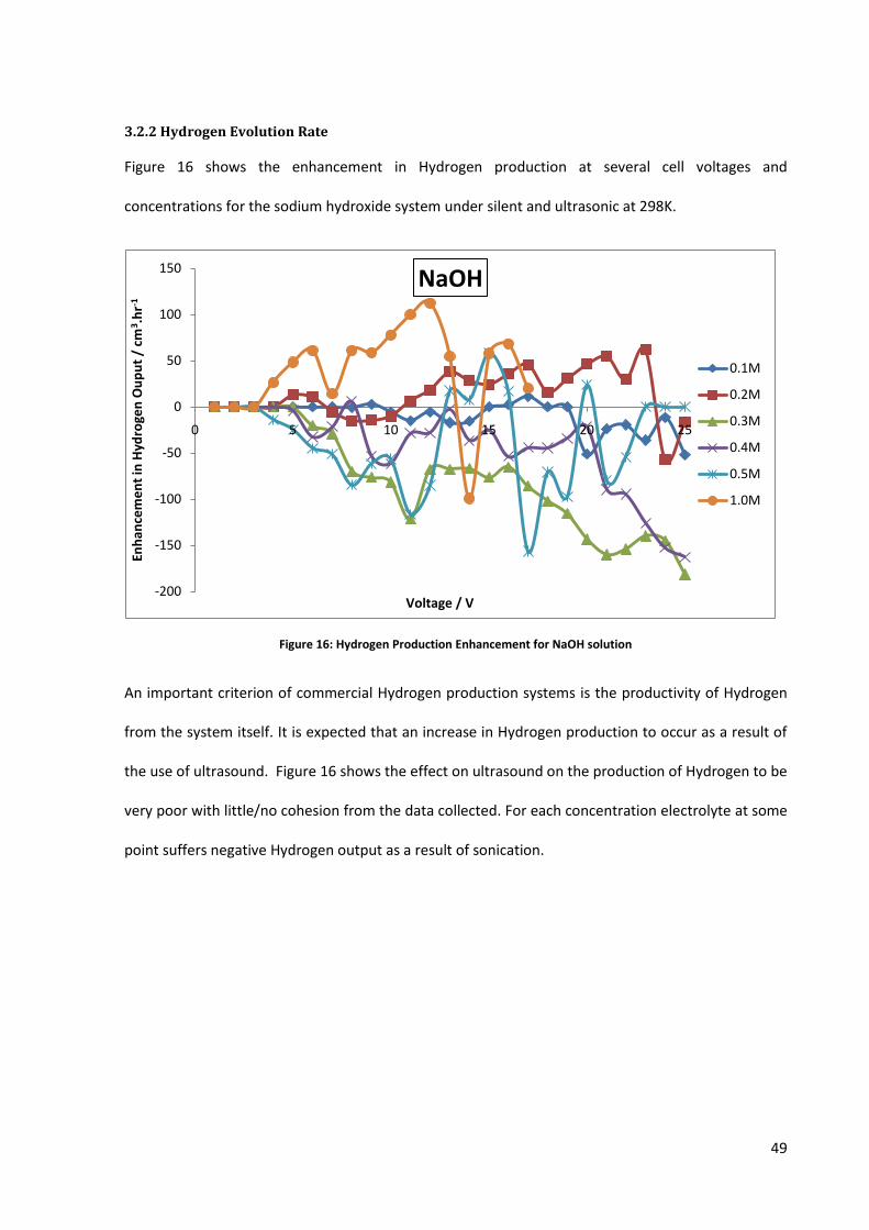
49
3.2.2 Hydrogen Evolution Rate
Figure 16 shows the enhancement in Hydrogen production at several cell voltages and
concentrations for the sodium hydroxide system under silent and ultrasonic at 298K.
Figure 16: Hydrogen Production Enhancement for NaOH solution
An important criterion of commercial Hydrogen production systems is the productivity of Hydrogen
from the system itself. It is expected that an increase in Hydrogen production to occur as a result of
the use of ultrasound. Figure 16 shows the effect on ultrasound on the production of Hydrogen to be
very poor with little/no cohesion from the data collected. For each concentration electrolyte at some
point suffers negative Hydrogen output as a result of sonication.
-200
-150
-100
-50
0
50
100
150
0 5 10 15 20 25
Enh
ance
me
nt
in H
ydro
gen
Ou
pu
t /
cm3 .
hr-1
Voltage / V
NaOH
0.1M
0.2M
0.3M
0.4M
0.5M
1.0M

50
Figure 17 shows an enhancement in Hydrogen production at several cell voltages as a result of the
introduction of ultrasound for sodium chloride in various concentrations at 298K.
Figure 17: Hydrogen Production Enhancement for NaCl solution
Figure 17 exhibits slightly more cohesive data than those shown in Figure 16. Only 0.4M and 1.0M
NaCl solutions show an enhancement in Hydrogen productivity, whilst for the other concentrations
of NaCl solutions show a decrease in Hydrogen production as a result of ultrasound. Once again, data
has only been recorded only once for these experiments, so is subject to unreliability.
-100
-50
0
50
100
150
0 5 10 15 20 25
Enh
ance
me
nt
in H
ydro
gen
Ou
pu
t /
cm3 .
hr-1
Voltage / V
NaCl
0.1M
0.2M
0.3M
0.4M
0.5M
1.0M

51
Figure 18 shows the enhancement in Hydrogen production at several cell voltages, at various
concentrations and at 298 K for the sulphuric acid system in the absence and presence of ultrasound.
Figure 18: Hydrogen Production Enhancement for H2SO4 solution
Figure 18 shows similar trends to Figure 16 and Figure 17 in that there is no visible increase in
Hydrogen production from the use of ultrasound. It would be expected to observe increases in
Hydrogen production for all concentrations used at various rates. Most of the concentrations
demonstrate detrimental effects in terms of Hydrogen production while only a few show a positive
impact.
Hydrogen production, for this investigation, is defined as the rate of which Hydrogen gas in produced
from the system. The production of Hydrogen increases with an increase in electrolyte
concentration. This is to be expected since there is an increase in number of charge carriers in the
solution, resulting in an enhanced mass transfer on the electrode surface induced by ultrasound
leading to an increase in Hydrogen production rate [79].
As shown in Figure 16, Figure 17 & Figure 18, the application of ultrasound to the system shows little
and even no improvement in the production of Hydrogen from the Sonoelectrochemical cell. From
-350
-300
-250
-200
-150
-100
-50
0
50
100
150
200
0 5 10 15 20 25
Enh
ance
me
nt
in H
ydro
gen
Ou
pu
t /
cm3 .
hr-1
Voltage / V
H2SO4
0.1M
0.2M
0.3M
0.4M
0.5M
1.0M

52
our observations here, whilst sonication is occurring, fewer bubbles are formed on the surface of the
electrodes due to the ultrasonic horn producing sonic waves through the solution. These ultrasonic
waves produce a ‘force’ on the electrodes surfaces, from which limited bubble formation on the
electrode surface. This limits the reaction rate of the Hydrogen ions (H+) and electrons (e-) on the
cathode surface and whilst the number of active sites is maintained, the ions and electrons have
difficultly reacting in the triple phase boundary on the electrode.
The data shown in Figure 16, Figure 17 & Figure 18 are not sufficient to draw any conclusions on
whether ultrasound enhances Hydrogen production. The repeatability of the experiments and use of
precision equipment, for example a flow meter calibrated to measure Hydrogen gas or better a Gas
Chromatographer (GC), instead of a measuring cylinder full of water being displaced by the Hydrogen
gas produced, could aid achieving conclusive results.

53
3.2.3 Hydrogen Efficiency Data
Figure 19 shows plots of efficiency enhancements of Hydrogen production at various cell voltages,
concentrations and 298 K for the sodium hydroxide system under silent and ultrasonic conditions.
Figure 19: Hydrogen Output Efficiency Enhancement for NaOH solution
Quantifying the efficiency of Hydrogen production is achieved by comparing the actual Hydrogen
production with the theoretical Hydrogen production from the ideal gas law (see above). Figure 19
shows a decrease in efficiency for all concentrations of NaOH, as a result of sonication, with the
highest loss being approximately 50% for the 0.3M NaOH solution.
-60
-50
-40
-30
-20
-10
0
10
20
0 5 10 15 20 25
Enh
ance
me
nt
in E
ffic
ien
cy /
%
Voltage / V
NaOH
0.1M
0.2M
0.3M
0.4M
0.5M
1.0M

54
Figure 20 shows plots of efficiency enhancements of Hydrogen production at various cell voltages,
concentrations and 298 K for the sodium chloride system under silent and ultrasonic conditions.
Figure 20: Hydrogen Output Efficiency Enhancement for NaCl solution
Figure 20 follows a similar trend to that in Figure 19, with negative gradients, implying that
ultrasound has a detrimental effect on Hydrogen production from electrolysis. 0.4M NaCl solution is
the only concentration that exhibits a positive increase in efficiency at any point, from the use of
ultrasound. Characterising the results from the data given in Figure 20 is not possible, so further work
needs to be carried out on this experimental set up to increase consistency and reliability of data.
-40
-35
-30
-25
-20
-15
-10
-5
0
5
10
0 5 10 15 20 25
Enh
ance
me
nt
in E
ffic
ien
cy /
%
Voltage / V
NaCl
0.1M
0.2M
0.3M
0.4M
0.5M
1.0M

55
Figure 21 shows plots of efficiency enhancements of Hydrogen production at various cell voltages,
concentrations and 298 K for the sulphuric acid system under silent and ultrasonic conditions.
Figure 21: Hydrogen Output Efficiency Enhancement for H2SO4 solution
Figure 21 clearly shows a decreasing efficiency for most of the electrolyte concentration used. This
observation is similar to the other electrolytes employed as shown in Figure 19 and Figure 20. 0.2M
H2SO4 exhibit an increase in efficiency under sonication to the electrolysis process. Further
experimental work is required to generate to produce consistent results with a higher level of
reliability.
The use of ultrasound to the electrochemical reactions results in a negative effect on the efficiency of
the system when compared to silent conditions. This observation is clearly shown in Figure 19, Figure
20 & Figure 21. As the previous section showed for Hydrogen production rates, the efficiency of
Hydrogen production shows similar trends in that, a decrease in Hydrogen production is observed
under sonication. Thus sonication has a negative effect on the efficiency of the system.
-35
-30
-25
-20
-15
-10
-5
0
5
10
15
20
0 5 10 15 20 25
Enh
ance
me
nt
in E
ffic
ien
cy /
%
Voltage / V
H2SO4
0.1M
0.2M
0.3M
0.4M
0.5M
1.0M

56
3.2.4 Energy Efficiency Data
Ideally an energy balance on the system should be carried out to calculate how much energy in the
form of Hydrogen is produced from the electrical energy used in the system. This process would
involve calculating the energy consumption i.e. kWh per m3 H2 produced at various cell voltages
under silent and sonicated conditions. The silent and sonicated systems can then be directly
compared to estimate a saving of energy consumption from sonicated systems compared with silent
systems.
In order to demonstrate whether this negative effect of ultrasound was not solely due to enhanced
mass-transfer, the investigation turns to the determination of the ultrasonic power used in our
conditions. It has been previously shown that the ultrasonic power may affect electrochemical
reactions.
3.2.5 Ultrasonic Power Determination
Ultrasound produces temperature fluctuations in solutions. These temperature changes (dT/dt) can
be used to calculate ultrasonic powers using Equation 24.
Power m p T (24
where m is the mass of the electrolyte solution (grams), Cp is the specific heat capacity of electrolyte
solution (J.g-1K-1), and ΔT is the change in temperature in the electrolyte solution (K).
A concentration of 0.1M was used for each electrolyte and Table 7 shows their corresponding
chemical and physical properties.
Densities (g cm
-3) Specific Heat (J g
-1 K
-1) Mass (g)
Water 1 4.18 1000
NaOH 2.13 3.331 1002.112
NaCl 2.165 3.98 1003.121
H2SO4 1.84 1.42 1004.5
Table 7: Chemical Properties for each electrolyte solution [94]

57
For each solution, the temperature rise was measured at 5 second intervals at various ultrasonic
amplitudes. The data were then plotted - Temperature vs. Time. The gradient at t = 0 s (dT/dt=0) was
then used to calculate the ultrasonic power (using Eq. 8).All ultrasonic powers used in this work are
shown in Table 8.
Ultrasound Power (W/cm2)
Amplitude / % 20 25 30 35 40
Water 43.9 65.9 109.9 87.9 131.8
NaOH 10.1 35.1 26.3 29.0 17.5
NaCl 10.5 25.2 10.5 16.8 15.7
H2SO4 12.4 15.0 11.2 18.7 26.2
Table 8: Ultrasonic Power Density Table
It is shown that increasing the amplitude of ultrasound largely increases the power of ultrasound in
the solutions as shown by Table 8. A solution containing only water, shows an increase in power
through the solution except in one case.
The electrolyte solutions, in most cases, show an increase in ultrasonic power as a result of
increasing the ultrasonic amplitude. Please note that all experiments were carried out once and
repeats are required to achieve reliability in the findings presented herein.
3.3 Erosion of the Electrodes
In all experiments, it was observed that, over prolonged periods of time the colour of the electrolytes
solution turned black as a result of erosion on the carbon electrodes. Acids and alkalines are highly
corrosive liquids, which is responsible for the degradation of the carbon electrodes as well the
intense effect of ultrasound induced by the implosion of cavitation bubbles on their surfaces.
The use of ultrasound to the solution increases this rate of erosion of the electrodes. NaCl and H2SO4
solutions, showed colour changes from colourless to black at a faster rate due to the mechanical
motion caused by the ultrasound. This faster rate of erosion was achieved by the force of ultrasonic
waves and cavitational events on the electrodes.

58
The erosion of the carbon electrodes is a serious issue with regards to the durability and life span of
the sonoelectrolytic cell. The use of alternative electrodes or electrolyte solutions must be used if
this process is ever to compete on a commercial scale.
3.4 Experiments with Industrial Electrolysers
3.4.1 Introduction
As part of my mini-project, an industrial electrolyser was tested on behalf of a company - Miromedia.
The principal difference between this unit and the cell researched in previous sections, is that it
produces HHO not H2. HHO is defined as a mixture of Hydrogen and oxygen gas, where no gas
separation has occurred from the electrolysis reaction.
The equipment was set up as illustrated in the Figure 22, and several experiments were carried out
to test the effect of varying the cell voltage across the electrolyser. Different concentrations of
potassium hydroxide solution were investigated to
characterise the conductivity of the solution and
the equivalent HHO production. A constant volume
of 300 cm3 of aqueous solution was used for each
experiment.
Two plastic tubes were connected from the side
arms of the electrolyser, to the underneath of the
larger plastic container. The plastic container was
placed at a greater height than the electrolyser
during operation, so that the KOH dissolved in
water solution entered the electrolyser through
the force of gravity.
Figure 22: Image of Experimental Setup

59
During operation, HHO gas was produced and exited the electrolyser through one of the connecting
tubes to the KOH solution reservoir. Simultaneously, the KOH solution flowed into the electrolyser
through the other tube as a result of gravity. This occurred when the pressure of HHO gas in the
electrolyser was great enough to create a force greater than that of gravity forcing the solution into
the electrolyser.
The nozzle on the bottom of the side tank, allowing the
connection from the main reservoir to the side tank, has
been poorly manufactured so suffers from a small leak of
distilled water from the side tank reservoir (shown in Figure
23). The joining of the side tank and the main reservoir was
achieved using masking tape. The only other connection
between the two reservoirs is a plastic tube which allows
the flow of HHO gas produced. It is suggested that the two
reservoirs should be secured together by stronger means
than just using masking tape.
The purpose of the side tank is defined for HHO gas cooling. However, it can be more suitably
described as a pressure relief vessel. Safety for the user is paramount and if there was a pressure
surge in the system, it would be favourable that the smaller vessel, containing distilled water,
ruptured than the larger vessel containing the alkali solution. This is achieved by the connection via
tubing of the main reservoir to the side tank.
Various concentrations of KOH solution were used characterise the electrochemical behaviour in
terms of the corresponding current flow. As well as measuring the flow of current through the
electrolyser, the flow rate of HHO being produced was also measured. It is expected that as the
current flowing through the solution increases, the rate of gas production will increase also.
Figure 23: Image showing small leak on side tank

60
3.4.2 Data Analysis
Figure 24 shows the flow of current through the electrolyser at various cell voltages at 298K.
Figure 24: Decomposition Curves for KOH solution
The graph shows, as expected, that with increasing cell voltage, the corresponding flow of current
also increases. When extra electrolyte (KOH) is added to the solution e.g. increasing the
concentration causes an increase in current flow as a result of further charge carriers in the solution,
the conductivity eventually reaches a maximum, where no further addition of electrolyte is
necessary.
The results in Figure 24 show a linear increase in current in the range [0-10 V] and thereafter, the
rate of current increase occurs at a faster rate. This could be due to possible reasons, but from our
general observations, during operation when a cell voltage was applied, the current would steadily
decrease over time, and then rapidly increase simultaneously with HHO bubbles discharged from the
electrolyser.
During operation, current is flowing and bubbles are forming on the surface of the electrodes. This
results in a decrease in surface area on the electrode surface, so the current steadily decreases (i.e.
0
2000
4000
6000
8000
10000
0 2 4 6 8 10 12 14 16
Cu
rren
t /
mA
Voltage / V
IV Curves
0.1M KOH
0.3M KOH
0.5M KOH

61
increase in bubble resistance/overpotential). When the pressure is building up in the electrolyser,
this results in a force greater than that from gravity forcing the solution into the electrolyser, the
coalesced HHO bubbles release from the electrode surface and leave the electrolyser unit. This
release results in a rapid increase in current flow hence the available surface area for current to flow
dramatically increases (i.e. decrease in bubble resistance/overpotential).
The decomposition voltages are calculated from Figure 24 and shown in Table 8.
Electrolyte Concentration
(mol.dm-3)
Decomposition
Voltage (V)
KOH
0.1 2.81
0.3 1.50
0.5 2.73
Table 9: Decomposition Voltages for Industrial Electrolyser
Table 9 shows that the industrial electrolyser has similar overpotentials as the Sonoelectrochemical
cell under investigation herein (Table 4). A concentration of 0.3M KOH solution leads to a
decomposition voltage of 1.5V. This figure suggests that an overpotential of approximately 0.3V, and
considering stainless steel, the material of the electrode in this electrolyser, has an activation
overpotential greater than 0.3V, and taking into account the ohmic overpotential in the solution,
further experiments are required to test the reliability of this data.

62
Figure 25 shows how the flow rate of produced HHO is affected at various cell voltages at 298K.
Figure 25: HHO Production for KOH solution
Figure 25 shows similar trends to the conductivity characteristics, in that, HHO production increases
with cell voltage. As the concentration of KOH solution increases, the rate of HHO production
increases. However, 0.3M and 0.5M solutions of KOH show very similar production rates of HHO. It
would be expected that 0.5M KOH has a higher production rate of HHO than 0.3M, but the data
obtained from experimentation shows otherwise.
It can be concluded that there is an optimum rate at where HHO can be produced. This is the result
of limited space in the electrolyser where the evolution of gas bubbles, the coalescence of these
bubbles and then the subsequent release of these bubbles when the upward force is greater than
the force of liquid entering the electrolyser occurs. This is the optimum production rate, and any
additional electrolyte will not result in any further increase in production rate.
0
1
2
3
4
5
6
7
8
0 5 10 15
Flo
w R
ate
/ cm
3.s
-1
Voltage / V
Productivity Curves
0.1M KOH
0.3M KOH
0.5M KOH

63
4. CONCLUSIONS
Initial experiments in this investigation involved characterising the electrochemical properties of the
various electrolyte solutions. The purpose of these experiments was to measure the electrical
conductivity of each electrolyte solution and therefore calculate the various decomposition cell
voltages.
The results obtained from the electrochemical reactions show that increasing the voltage across the
electrolyte solution increases the subsequent flow of current between the electrodes. It is also
shown that increasing concentrations of each electrolyte results in an increase in flow of current
through the solution. This is to be expected due to the increase in number of charge carriers, with
increasing concentration. The data collected and analysed shows that the introduction of ultrasound
to the solution increase the flow of current through the solution.
From comparing the different electrolytes at 1.0M concentration, the data shows, as expected
considering the ionic make up, that sulphuric acid has a better electrolytic conductivity than sodium
hydroxide and sodium chloride respectively. These conclusions were achieved from using basic
laboratory equipment and an ultrasonic bath as stated in Chapter 3.
The customised glassware enabled the analysis of ultrasound on the production of hydrogen to
occur. The electrochemical data from the customised glassware shows similar trends to that shown
with the preliminary experiments.
The productivity data follows a similar trend to that of the electrochemical data with increasing
concentration resulting in an increase yield of Hydrogen, but the comparison of silent and sonicated
yields show that sonication has, in most cases, a negative effect on Hydrogen production.

64
Once again, when comparing the efficiency of a silent to a sonicated system, the expected
enhancement from the use of ultrasound, only results in a decrease in efficiency for all electrolytes
employed.
Previous findings from the literature have shown an increase in Hydrogen production rates from the
sonicated solutions, but in this investigation our observations showed otherwise.
A possible explanation for our observations could be due to the large volume of solution used. Here,
the electrolyte solution volume was kept constant at 1,000cm3, which is a large volume of liquid
whereby ‘cavitation’ in the electrolyte solution may be hindering mass transfer on the electrode
surface. Previous studies in this field were performed in smaller volumes of electrolyte solution
(<100cm3) than used in this investigation, and a reduction in reaction volume and modification of
reaction vessel geometry are important parameters.
In order to reduce resistances in the electrolytic system, solutions usually undergo a process called
‘degassing’. This involves purging the electrolyte solution with non reactive gases, such as nitrogen or
argon, to remove any air or gases dissolved in the solution. In this experiment degassing was not
performed for all electrolyte solutions used. However, future investigations in this field should
include degassing of the electrolyte solutions allowing subsequent comparison of electrochemical
behaviour to quantify any improvement (reduction of resistance) in the system.
Commercial electrolysers usually operate at 1.8V-2.0V. Ideally, they would need to operate at 1.23V
but due to overpotentials (due to the electrodes & electrolytes), the electrolysers would need to
operate at higher cell voltages. Since the decomposition cell voltages shown herein are
approximately 3V, a clear diminishment in overpotential in the system need to be achieved, in order
to be commercially viable.

65
The carbon electrodes in this research have high activation potentials [0.62V for the Hydrogen
evolution reaction (HER) and 0.95V for the oxygen evolution reaction (ORR)] when compared to
materials like platinum (0.07V for the HER and 0.77V for the ORR) and palladium (0.07V for the HER
and 0.93V for the ORR).
The purpose of this research was to use cost-effective materials, such as carbon, but on the other
hand they produce higher overpotentials than precious metals (platinum). The exact opposite is true
for platinum and palladium, higher costs and lower overpotentials. Finding a balance between
electrode material cost and activation overpotential is an area of active research.
Maximising the productivity of Hydrogen from ‘water’ electrolysis is an important factor for
commercial Hydrogen production systems. The contact area between the electrodes and the
electrolyte solution is the critical parameter in determining the number of actives sites available for
the evolution of Hydrogen gas to occur. It is recommended that research is undertaken in this area,
linked in with various reaction vessel geometries to attempt in increasing the contact area between
the electrodes and the liquid solution for facile electron transfer.
The 6-month research presented herein was carried out in a closed vessel (batch operation). This
could be compared with continuous flow as used by Li et al. [87]. The flow through of solution from a
supply tank to an electrolysis unit could increase mass transfer on the surface of the electrodes and if
only a small volume at a time is subjected to ultrasound in the electrolysis unit, this could
demonstrate whether ultrasound has a beneficial effect on the rate of Hydrogen production from
electrolysis.
Future investigation in this field may benefit from measurement of flow rate using a flowmeter
instead of a measuring cylinder and a stopwatch and a GC. The use a digital flowmeter would be
greatly beneficial and would eliminate human error caused by reading values on the measuring
cylinder at eye level.

66
The modification of the sonication distance as
shown in Figure 26 is another field worth
investigating to see whether this has any effect
on the enhancement of electrolysis through the
introduction of ultrasound.
The dilemma of carrying out Sonoelectrochemical
research on small scale, and commercial
Hydrogen production systems require large
volume so high contact areas of electrode and
electrolyte can be achieved. One method of potentially overcoming this problem, and requiring
research, is the use of localised sonication in the system.
The use of PEM electrolysis would be beneficial when compared to alkaline electrolysis, since there
are no acidic/alkaline solutions used in PEM electrolysis. This would result in easier handling for the
personnel operating the equipment, whether that is a scientist or a member of the public using the
equipment commercially. The electrodes (carbon), which this research has shown, suffer from
erosion when subjected to acid/alkaline conditions. Using water instead of these corrosive solutions
will increase the lifespan of the electrodes and their durability.
4.1 Comparison for Industrial Electrolyser and Sonoelectrochemical Cell From the data presented it is clear that using KOH solution into an electrolyser and applying an
electrical current results in HHO production. Increasing the cell voltage and electrolyte
concentration, result in an increase in HHO production up to an optimal point. Car batteries operate
at 12V and if the electrolyser were connected to them for HHO injection into an internal combustion
engine (ICE), an optimum HHO production would occur when using an approximate concentration of
0.3M KOH solution.
Figure 26: Diagram defining the Sonication Distance

67
These observations suggest that using 5g of KOH for every 300cm3 of distilled water added to the
main reservoir is recommended. The total volume of the electrolyte solution (to add) is dependent
on the rate of usage of the KOH solution and how often the reservoir requires refilling. Any excess
KOH will not be dangerous or harmful to the electrolyser; it will not improve the performance
further.
A direct comparison between the Miromedia electrolyser unit and the Sonoelectrochemical cell is
difficult since the two systems have different gas composition outputs. The Miromedia electrolyser
produces a mixture of Hydrogen and oxygen, whilst the Sonoelectrochemical cell produces H2 only
(and in some case Cl2).
These are not the only fundamental differences between the experiments observed here and the
commercial unit. The Miromedia unit uses stainless steel (SS 316) electrodes and potassium
hydroxide electrolyte, whilst the experiments previously performed in this report use carbon
electrodes and sodium hydroxide solutions. Stainless steel is a better electrode material than carbon
since it has a lower activation overpotential, thus creating less resistance in the flow of electrons
through the electrolyte. Potassium hydroxide is a better electrolyte than sodium hydroxide for this
purpose, as it is more electrically conductive due to the increased number of charge carriers in
solution.
More importantly, the surface area of the electrodes in the Miromedia electrolyser is not known.
This makes it impossible to draw any direct comparisons with the Sonoelectrochemical cell. Knowing
the contact area allows the conversion of the current to current density, which makes the results
independent of contact area. If the contact area, the electrolyte and the electrolyte concentration
were kept the same, a conductivity performance comparison of the stainless steel and carbon
electrodes could occur.

68
Hydrogen gas productivity cannot be compared since the two units produce different gases. The
Sonoelectrochemical cell separates the Hydrogen and oxygen gas, whilst the Miromedia electrolyser
does not. The only way that the gas productivity can be compared is to combine the Hydrogen and
oxygen gas resultant flows from the Sonoelectrochemical cell.

69
5. FUTURE WORK
Most importantly for future work, the need to repetition of experiments is a vital requirement. The
work shown herein severely lacks reliability from which no defining conclusions can be drawn. A
limited time-scale has made repetition not possible at this time, but if it was available multiple
repetition of each experiment is a must. This would also enable statistical analysis of the data
collected calculate averages and carry out an error analysis.
To improve the process presented above, the use of localised sonication in bulk solutions must be
investigated. Using small solutions, which most previous sonoelectrochemical research has used,
would not produce Hydrogen on a scale for commercial needs. Since the volume of the electrolyte
solution used is very small, there will be a very small contact area between the electrode surface and
the electrolyte solution itself. The small contact area results in fewer active sites for Hydrogen
production to occur.
5.1 Electrolytes
The electrolytes used in this project are fairly weak in comparison to others such as potassium
hydroxide because they are more electrically conductive than sodium hydroxide.
Purging of each solution with nitrogen or argon for a fixed period of time before and/or during the
electrolysis process would improve the production rate of Hydrogen. This would reduce the volume
of air in solution, and reduce ohmic resistance in the solution.
Another possible electrolyte that has been investigated is urea. Urea is the main component of urine
and is produced from humans in large quantities every day. The utilisation of a waste product for
Hydrogen production could be very economically and environmentally beneficial, rather than using
harmful acids/bases, which require costly manufacturing and careful handling.

70
Another alternative is the use of a solid polymer electrolyte in the form of a membrane. This removes
the needs for a liquid electrolyte (acid/base) and can produce Hydrogen via electrolysis through only
water. If electrolyser technology is used on a commercial scale in the future, it would be more
convenient for the public to have to use only water, rather than handling acids and alkalines which
are potential dangers to public health.
5.2 Electrode Parameters
The electrodes have many parameters that can be varied. The use of different material electrodes
can be investigated. Each material has different properties, such as conductivity and microstructure.
The activation overpotential of each material will be of particular interest, since materials with the
lowest activation overpotential will enable the electrolysis reaction to proceed at lower potentials.
The surface area of the electrode in contact with the electrolyte solution is another important factor
in electrolysis. Maximising the surface area of electrodes results in more active sites for current flow
in the solution and increases the rate of Hydrogen gas production.
The distance between the cathode and anode electrodes affects the productivity of Hydrogen
production. When the electrons move through the solution, there is ohmic resistance in the solution
and the closer the electrodes are together, the less resistance when transferring from anode to
cathode.
5.3 Electrolyte Temperature
The temperature of the electrolyte solution will affect the production of Hydrogen, since increasing
the temperature of a solution increases the energy of the ions in solution and they become more
energetic, thus reducing the levels of resistance in the solution. An increase in pressure has a similar
effect on the solution and applying a pressure to the solution removes the bubbles from the surface

71
of the electrodes at a faster rate than waiting for bubbles to coalesce and then implode on the
surface of the solution.
5.4 Ultrasonic Parameters
The parameters of the ultrasound applied to the solution can affect the production rate of
ultrasound also. Increasing the amplitude of ultrasound will directly increase the flow of current
through the solution and this should result in an increase in production of Hydrogen gas.
The frequency of the ultrasound could be adjusted to see what effect this has on the production of
Hydrogen; most particularly to the natural resonant frequency of water to see what effect sonication
at this frequency has on the productivity. The distance from the electrodes to the source of
sonication has been identified in this report as a serious area that requires further research and the
closer they are together, the greater the impact that the ultrasound will have on the electrolysis
reaction.

72
6. REFERENCES
1. Veziroglu, T.N. and S. Sahin, 21st Century's energy: Hydrogen energy system. Energy Conversion and Management, 2008. 49(7): p. 1820-1831.
2. www.Direct.gov. Brief History of Climate Change. 2009 [cited 2009 15-11-2009]. 3. Lattin, W.C. and V.P. Utgikar, Transition to hydrogen economy in the United States: A 2006
status report. International Journal of Hydrogen Energy, 2007. 32(15): p. 3230-3237. 4. Florides, G.A. and P. Christodoulides, Global warming and carbon dioxide through sciences.
Environment International, 2009. 35(2): p. 390-401. 5. http://www.chemie-im-alltag.de/english/articles/0024/Greenhouse.jpg. Diagram of
Greenhouse Effect. 2009 [cited 2009 15-11-2009]. 6. Garrett, C.W., On global climate change, carbon dioxide, and fossil fuel combustion. Progress
in Energy and Combustion Science, 1992. 18(5): p. 369-407. 7. Jain, P.C., Greenhouse effect and climate change: scientific basis and overview. Renewable
Energy. 3(4-5): p. 403-420. 8. Smith, I.M., CO2 and climatic change: An overview of the science. Energy Conversion and
Management. 34(9-11): p. 729-735. 9. Susskind, C., Henry Cavendish, electrician. Journal of the Franklin Institute, 1950. 249(3): p.
181-187. 10. Sørensen, B., Hydrogen and Fuel Cells - Emerging technologies and applications. Sustainable
World. 2005: Elsevier Academic Press. 450. 11. Despic, A.R., Electrochemistry of John O'Mara Bockris--retrospect and prospects.
Electrochimica Acta, 1994. 39(11-12): p. 1467-1469. 12. Lau, C.E.G.P.F., Advances in Hydrogen Energy. 2000, New York: Springer. 192. 13. Balat, M., Potential importance of hydrogen as a future solution to environmental and
transportation problems. International Journal of Hydrogen Energy, 2008. 33(15): p. 4013-4029.
14. Barbir, F., Transition to renewable energy systems with hydrogen as an energy carrier. Energy, 2009. 34(3): p. 308-312.
15. Crowl, D.A. and Y.-D. Jo, The hazards and risks of hydrogen. Journal of Loss Prevention in the Process Industries, 2007. 20(2): p. 158-164.
16. Ltd, H.-F. Diagram of Flammability Range of Hydrogen and other Fuels. 2007; Available from: http://www.hydrogen-fc.com/flammability-range-on-hydrogen-and-other-fuel/.
17. Winter, C.-J., Hydrogen energy -- Abundant, efficient, clean: A debate over the energy-system-of-change. International Journal of Hydrogen Energy, 2009. 34(14, Supplement 1): p. S1-S52.
18. Ramesohl, S. and F. Merten, Energy system aspects of hydrogen as an alternative fuel in transport. Energy Policy, 2006. 34(11): p. 1251-1259.
19. Elam, C.C., et al., Realizing the hydrogen future: the International Energy Agency's efforts to advance hydrogen energy technologies. International Journal of Hydrogen Energy, 2003. 28(6): p. 601-607.
20. Moriarty, P. and D. Honnery, Hydrogen's role in an uncertain energy future. International Journal of Hydrogen Energy, 2009. 34(1): p. 31-39.
21. Barbir, F., PEM electrolysis for production of hydrogen from renewable energy sources. Solar Energy, 2005. 78(5): p. 661-669.
22. Jensen, S.H., P.H. Larsen, and M. Mogensen, Hydrogen and synthetic fuel production from renewable energy sources. International Journal of Hydrogen Energy, 2007. 32(15): p. 3253-3257.

73
23. Srinivasan, S. and F.J. Salzano, Prospects for hydrogen production by water electrolysis to be competitive with conventional methods. International Journal of Hydrogen Energy, 1977. 2(1): p. 53-59.
24. Kothari, R., D. Buddhi, and R.L. Sawhney, Studies on the effect of temperature of the electrolytes on the rate of production of hydrogen. International Journal of Hydrogen Energy, 2005. 30(3): p. 261-263.
25. Arashi, H., H. Naito, and H. Miura, Hydrogen production from high-temperature steam electrolysis using solar energy. International Journal of Hydrogen Energy, 1991. 16(9): p. 603-608.
26. Zhang, B., et al., Hydrogen production from steam reforming of ethanol and glycerol over ceria-supported metal catalysts. International Journal of Hydrogen Energy, 2007. 32(13): p. 2367-2373.
27. Levent, M., D. J. Gunn, and M. Ali El-Bousiffi, Production of hydrogen-rich gases from steam reforming of methane in an automatic catalytic microreactor. International Journal of Hydrogen Energy, 2003. 28(9): p. 945-959.
28. Melis, A. and M.R. Melnicki, Integrated biological hydrogen production. International Journal of Hydrogen Energy, 2006. 31(11): p. 1563-1573.
29. Skjånes, K., et al., H2 production from marine and freshwater species of green algae during sulfur deprivation and considerations for bioreactor design. International Journal of Hydrogen Energy, 2008. 33(2): p. 511-521.
30. Roy, R., Rao, M.L., Kanzius, J., Observations of polarised RF radiation catalysis of dissociation of H2O-NaCl solutions. Materials Research Innovations, 2008. 12: p. 3-6.
31. Ahmed, S., et al., Decomposition of hydrocarbons to hydrogen and carbon. Applied Catalysis A: General, 2009. 359(1-2): p. 1-24.
32. Cormos, C.-C., et al., Innovative concepts for hydrogen production processes based on coal gasification with CO2 capture. International Journal of Hydrogen Energy, 2008. 33(4): p. 1286-1294.
33. Mueller-Langer, F., et al., Techno-economic assessment of hydrogen production processes for the hydrogen economy for the short and medium term. International Journal of Hydrogen Energy, 2007. 32(16): p. 3797-3810.
34. Hallenbeck, P.C., Fermentative hydrogen production: Principles, progress, and prognosis. International Journal of Hydrogen Energy, 2009. 34(17): p. 7379-7389.
35. Kruger, P., Appropriate technologies for large-scale production of electricity and hydrogen fuel. International Journal of Hydrogen Energy, 2008. 33(21): p. 5881-5886.
36. Baykara, S.Z., Hydrogen production by direct solar thermal decomposition of water, possibilities for improvement of process efficiency. International Journal of Hydrogen Energy, 2004. 29(14): p. 1451-1458.
37. Soler, L., et al., Aluminum and aluminum alloys as sources of hydrogen for fuel cell applications. Journal of Power Sources, 2007. 169(1): p. 144-149.
38. Holladay, J.D., et al., An overview of hydrogen production technologies. Catalysis Today, 2009. 139(4): p. 244-260.
39. Getoff, N., Photoelectrochemical and photocatalytic methods of hydrogen production: A short review. International Journal of Hydrogen Energy, 1990. 15(6): p. 407-417.
40. Center, F.S.E. Diagram of Hydrogen Production Pathways. Available from: http://www.fsec.ucf.edu/en/consumer/hydrogen/basics/production.htm.
41. Andújar, J.M. and F. Segura, Fuel cells: History and updating. A walk along two centuries. Renewable and Sustainable Energy Reviews, 2009. 13(9): p. 2309-2322.
42. T.J. Mason, J.P.L.a.D.J.W., Sonoelectrochemistry. Ultrasonics, 1990. 28: p. 333-337. 43. Courtney, J., Diagram of MEA. 2010. p. Poster Presentation, Japan.

74
44. Levie, R.d., What’s in a Name? Journal of Chemical Education, 2000. 7(5): p. 610-612. 45. Toftlund, H., Very early observations on fuel cells. Ionics, 2001. 7(3): p. 161-164. 46. Laboratory, M.L.-N.H.M.F. Magnet Lab - National High Magnetic Field Laboratory - 1850-
1869. 2010 [cited 2010 29/09/2010]; Available from: http://www.magnet.fsu.edu/education/tutorials/timeline/1850-1869.html.
47. History, S. Dimitry Lachinov. [cited 2010 29/09/2010]; Available from: http://www.servinghistory.com/topics/Dmitry_Lachinov.
48. Laskin, J.B. and R.D. Feldwick, Recent development of large electrolytic hydrogen generators. International Journal of Hydrogen Energy, 1978. 3(3): p. 311-320.
49. Kreuter, W. and H. Hofmann, Electrolysis: The important energy transformer in a world of sustainable energy. International Journal of Hydrogen Energy, 1998. 23(8): p. 661-666.
50. Justi, E.W., Seventy years of Fuel Cell Research. British Journal of Applied Sciences, 1963. 14(12): p. 840.
51. Zuttel, A., Borgschulte, A., Schlapbach, L., Hydrogen as a Future Energy Carrier. 2008, Weinheim: Wiley.
52. Richards, J.W., Electrolysis of Water. The Electrical Section, 1905: p. 377-394. 53. Stojic, D.L., et al., Hydrogen generation from water electrolysis--possibilities of energy saving.
Journal of Power Sources, 2003. 118(1-2): p. 315-319. 54. Grigoriev, S.A., V.I. Porembsky, and V.N. Fateev, Pure hydrogen production by PEM
electrolysis for hydrogen energy. International Journal of Hydrogen Energy, 2006. 31(2): p. 171-175.
55. Madigan, N.A., et al., Effects of sonication on electrode surfaces and metal particles. Ultrasonics Sonochemistry, 1996. 3(3): p. S239-S247.
56. Mason, T.J., Sonochemistry and sonoprocessing: the link, the trends and (probably) the future. Ultrasonics Sonochemistry, 2003. 10(4-5): p. 175-179.
57. Mason, T.J., Sonochemistry and the environment - Providing a "green" link between chemistry, physics and engineering. Ultrasonics Sonochemistry, 2007. 14(4): p. 476-483.
58. Walton, D.J., L.D. Burke, and M.M. Murphy, Sonoelectrochemistry: Chlorine, hydrogen and oxygen evolution at platinised platinum. Electrochimica Acta, 1996. 41(17): p. 2747-2751.
59. Walton, D.J., et al., Ultrasonic enhancement of electrochemiluminescence. Electrochimica Acta, 1993. 38(2-3): p. 307-310.
60. González-García, J., et al., Current topics on sonoelectrochemistry. Ultrasonics, 2009. In Press, Corrected Proof.
61. Moriguchi, N.J., The effect of supersonic waves on chemical phenomena. Journal of the Chemical Society Japan, 1934(55): p. 749.
62. Nyborg, W.L.S., M. I. L. , Effects of acoustic microstreaming at electrodes. Proceedings of the 3rd International Congress on Acoustics, 1960, 1960: p. 346-348.
63. Zhang, H.H.C., L. A. , Effects of High-Intensity Ultrasound on Glassy-Carbon. Electrodes. Analytical Chemistry, 1993(65): p. 1552.
64. Compton, R.G., et al., Dual activation: coupling ultrasound to electrochemistry--an overview. Electrochimica Acta, 1997. 42(19): p. 2919-2927.
65. Klíma, J., C. Bernard, and C. Degrand, Sonoelectrochemistry: Effects of ultrasound on voltammetric measurements at a solid electrode. Journal of Electroanalytical Chemistry, 1994. 367(1-2): p. 297-300.
66. Hagan, C.R.S.C., L. A., Comparison of Hydrodynamic Voltammetry Implemented by Sonication to a Rotating-Disk Electrode. Analytical Chemistry, 1994. 66: p. 399.
67. Marken, F., J.C. Eklund, and R.G. Compton, Voltammetry in the presence of ultrasound: Can ultrasound modify heterogeneous electron transfer kinetics? Journal of Electroanalytical Chemistry, 1995. 395(1-2): p. 335-339.

75
68. Compton, R.G.E., J. C.; Page, S. D., Sonovoltammetry - Heterogeneous Electron -Transfer processes with coupled ultrasonically induced chemical-reaction. Journal Of Physical Chemistry, 1995(99): p. 4211-4214.
69. Pollet, B. Schematic of Ultrasonic Phenomena. 2007 [cited 2010 04/10/2010]; Available from: http://www.sonoelectrochemistry.com/.
70. Birkin, P.R.S.-M., S. , The effect of ultrasound on mass transport to a microelectrode. Journal of Electroanalytical Chemistry, 1996(416): p. 1807.
71. Birkin, P.R. and S. Silva-Martinez, A study on the effect of ultrasound on electrochemical phenomena. Ultrasonics Sonochemistry, 1997. 4(2): p. 121-122.
72. Birkin, P.R.O., D. G.; Leighton, T. G. , A novel dual microelectrode for investigating mass transfer and surface erosion caused by cavitation. Electrochemistry Communications, 2004(6): p. 1174.
73. Birkin, P.R.O., D. G.; Leighton, T. G., Experimental and theoretical characterisation of sonochemical cells - Part 2 Cell disruptors (Ultrasonic horns) and cavity cluster collapse. Physical Chemistry Chemical Physics, 2005(7): p. 530.
74. Maisonhaute, E.W., P. C.; Compton, R. G. , Surface acoustic cavitation understood via nanosecond electrochemistry. Journal Of Physical Chemistry, 2001(105): p. 12087-12091.
75. Birkin, P.R.P., J. F.; Leighton, T. G.; Vincüotte, A. M. L., Cathodic Electrochemical Detection of Sonochemical Radical Products. Analytical Chemistry, 2002(74): p. 2584.
76. Gaitan, D.F.C., L. A.; Church, C. C.; Roy, R. A. , Sonoluminescence and bubble dynamics for a single, stable, cavitation bubble. Journal of the Acoustical Society of America, 1992. 91(6): p. 3166.
77. Weissler, A.C., H. W.; Snyder, S., Chemical Effect of Ultrasonic Waves: Oxidation of Potassium Iodide Solution by Carbon Tetrachloride. Journal of the American Chemical Society, 1950. 4(72): p. 1769-1775.
78. Weissler, A., Formation of Hydrogen Peroxide by Ultrasonic Waves: Free Radicals. Journal of the American Chemical Society, 1959. 5(81): p. 1077-1081.
79. Birkin, P.R.P., J. F.; Leighton, T. G., Electrochemical evidence of H radicals produced by ultrasound. Journal of the Chemical Society Chemical Communications, 2001.
80. Birkin, P.R.O.C., R.; Rapple, C.; Silva-Martinez, S. , Electrochemical measurement of erosion from individual cavitation generated from continuous ultrasound. Journal of Chemical Society, 1998(94): p. 3365.
81. Galloway, W.J., An Experimental Study of Acoustically Induced Cavitation in Liquids. Journal of the Acoustical Society of America, 1954(26): p. 849.
82. Cataldo, F., Effects of ultrasound on the yield of hydrogen and chlorine during electrolysis of aqueous solutions of NaCl or HCl. Journal of Electroanalytical Chemistry, 1992. 332: p. 325-331.
83. D. J. Walton, L.D.B., M. M. Murphy, Sonoelectrochemistry: Chlorine, Hydrogen and Oxygen Evolution at Platinised Platinum. Electrochimica Acta, 1996. 41: p. 2747-2751.
84. H.N. McMurray, D.A.W., B.P. Wilson, Hydrogen Evolution and Oxygen Reduction at Titanium Sonotrode. Chemical Communications, 1998: p. 887-888.
85. C. Burdischak, C.H., R.L. Opila, Electroanalytical Effects of ultrasound on hydrogen evolution reaction in KOH. 2008, University of Delaware.
86. Sasikala, R., O.D. Jayakumar, and S.K. Kulshreshtha, Enhanced hydrogen generation by particles during sonochemical decomposition of water. Ultrasonics Sonochemistry, 2007. 14(2): p. 153-156.
87. Li, S.-D., C.-C. Wang, and C.-Y. Chen, Water electrolysis in the presence of an ultrasonic field. Electrochimica Acta, 2009. 54(15): p. 3877-3883.

76
88. Thomas, R., et al., Trap-governed hydrogen diffusivity and uptake capacity in ultrahigh-strength AERMET 100 steel. Metallurgical and Materials Transactions A, 2002. 33(7): p. 1991-2004.
89. Melsheimer, J. and D. Ziegler, The oxygen electrode reaction in acid solutions on RuO2 electrodes prepared by the thermal decomposition method. Thin Solid Films, 1988. 163: p. 301-308.
90. Shi, K., et al., Structural studies of electrochemically activated glassy carbon electrode: Effects of chloride anion on the redox responses of copper deposition. Electrochimica Acta, 2007. 52(19): p. 5907-5913.

77
7. APPENDICES
7.1 Appendix I - Data Tables
7.1.1 Preliminary Experiments
Silent
NaOH
V mA V mA V mA V mA V mA V mA
1 0.5 0.5 1 0.5 1 0.5 2 0.5 1 0.25 0
2 6 1 1 1 3 1 3 1 3 0.5 1
3 28 1.5 2 1.5 5 1.5 4 1.5 5 0.75 1
4 69 2 4 2 7 2 7 2 7 1 2
5 109.5 2.5 17 2.5 23 2.5 25 2.5 32 1.25 2
6 152.5 3 43 3 58 3 62 3 76 1.5 3
7 198 3.5 75 3.5 102 3.5 102 3.5 133 1.75 5
8 230 4 107 4 150 4 149 4 201 2 8
9 275.5 4.5 139 4.5 195 4.5 201 4.5 275 2.25 22
10 318 5 172 5 246 5 260 5 360 2.5 52
11 363.5 5.5 209 5.5 300 5.5 319 5.5 441 2.75 92
12 408.5 6 246 6 355 6 381 6 522 3 135
13 452 6.5 284 6.5 411 6.5 443 6.5 606 3.25 180
14 497 7 322 7 466 7 511 7 691 3.5 230
15 541 7.5 361 7.5 524 7.5 580 7.5 775 3.75 280
16 596 8 400 8 581 8 649 8 859 4 336
17 645 8.5 439 8.5 638 8.5 722 8.5 946 4.25 398
18 694.5 9 477 9 697 9 789 9 1035 4.5 459
19 744.5 9.5 516 9.5 755 9.5 864 9.5 1122 4.75 523
20 794 10 556 10 805 10 934 10 1210 5 590
21 847 10.5 596 10.5 865 10.5 1006 10.5 1298 5.25 655
22 897.5 11 634 11 923 11 1079 11 1390 5.5 721
23 951.5 11.5 672 11.5 987 11.5 1167 11.5 1487 5.75 789
24 1007.5 12 706 12 1045 12 1240 12 1578 6 856
25 1065.5 12.5 739 12.5 1107 12.5 1312 12.5 1670 6.25 923
13 778 13 1172 13 1387 13 1764 6.5 993
13.5 817 13.5 1235 13.5 1462 13.5 1858 6.75 1062
14 858 14 1302 14 1539 14 1955 7 1132
14.5 898 14.5 1361 14.5 1620 7.25 1201
15 937 15 1426 15 1700 7.5 1271
15.5 978 15.5 1490 15.5 1780 7.75 1341
16 1020 16 1556 16 1863 8 1411
16.5 1063 16.5 1629 16.5 1945 8.25 1483
17 1106 17 1700 8.5 1554
17.5 1151 17.5 1777 8.75 1624
18 1192 18 1846 9 1699
18.5 1235 18.5 1910 9.25 1765
19 1278 19 1984 9.5 1838
19.5 1315 9.75 1904
20 1367 10 1976
20.5 1401
21 1448
21.5 1483
22 1523
22.5 1568 3.5 cm
23 1601 0.15 cm
23.5 1643
24 1684 1.667008 cm2
24.5 1706
25 1745
0.5M 1.0M
Electrode Contact Length
Electrode Diameter
Contact Area
0.1M 0.2M 0.3M 0.4M
Figure 27: Table of Voltage Current Data for NaOH

78
NaCl
V mA V mA V mA V mA V mA V mA
1 1 0.5 2 0.5 0 0.5 1 0.5 1 0.25 0
2 4 1 3 1 2 1 5 1 3 0.5 0
3 8 1.5 6 1.5 5 1.5 11 1.5 12 0.75 0
4 23 2 7 2 7 2 23 2 31 1 0
5 44 2.5 11 2.5 9 2.5 40 2.5 44 1.25 0
6 66 3 14 3 14 3 57 3 55 1.5 0
7 89 3.5 25 3.5 31 3.5 74 3.5 74 1.75 0
8 112 4 42 4 53 4 92 4 100 2 0
9 136 4.5 62 4.5 77 4.5 111 4.5 129 2.25 2
10 160 5 83 5 102 5 130 5 141 2.5 5
11 184 5.5 104 5.5 127 5.5 149 5.5 195 2.75 10
12 208 6 125 6 154 6 181 6 229 3 20
13 234 6.5 147 6.5 181 6.5 214 6.5 262 3.25 36
14 259 7 169 7 209 7 247 7 297 3.5 57
15 285 7.5 192 7.5 236 7.5 281 7.5 329 3.75 81
16 310 8 214 8 264 8 316 8 363 4 109
17 336 8.5 237 8.5 293 8.5 351 8.5 399 4.25 138
18 362 9 260 9 320 9 386 9 435 4.5 168
19 389 9.5 283 9.5 349 9.5 421 9.5 471 4.75 199
20 414 10 305 10 378 10 456 10 510 5 230
21 439 10.5 328 10.5 407 10.5 492 10.5 552 5.25 263
22 465 11 350 11 435 11 527 11 600 5.5 295
23 491 11.5 374 11.5 464 11.5 564 11.5 645 5.75 328
24 519 12 397 12 495 12 600 12 693 6 361
25 547 12.5 420 12.5 514 12.5 636 12.5 739 6.25 394
13 444 13 544 13 673 13 775 6.5 428
13.5 468 13.5 573 13.5 709 13.5 821 6.75 461
14 492 14 602 14 746 14 867 7 494
14.5 515 14.5 635 14.5 784 14.5 913 7.25 529
15 539 15 662 15 812 15 952 7.5 563
15.5 564 15.5 692 15.5 850 15.5 1000 7.75 594
16 589 16 723 16 888 16 1044 8 625
16.5 615 16.5 754 16.5 924 16.5 1092 8.25 661
17 638 17 787 17 961 17 1136 8.5 694
17.5 665 17.5 815 17.5 999 17.5 1180 8.75 728
18 690 18 847 18 1035 18 1223 9 761
18.5 714 18.5 878 18.5 1074 18.5 1276 9.25 794
19 740 19 908 19 1109 19 1328 9.5 827
19.5 767 19.5 935 19.5 1146 19.5 1375 9.75 859
20 789 20 966 20 1184 20 1423 10 894
20.5 814 20.5 995 20.5 1220 20.5 1469 10.25 928
21 843 21 1024 21 1259 21 1516 10.5 963
21.5 867 21.5 1056 21.5 1293 21.5 1559 10.75 997
22 892 22 1084 22 1324 22 1602 11 1030
22.5 915 22.5 1118 22.5 1361 22.5 1648 11.25 1064
23 941 23 1145 23 1398 23 1694 11.5 1097
23.5 968 23.5 1172 23.5 1434 23.5 1742 11.75 1125
24 995 24 1204 24 1472 24 1790 12 1159
24.5 1021 24.5 1237 24.5 1510 24.5 1833 12.25 1194
25 1046 25 1268 25 1548 25 1881 12.5 1227
12.75 1262
13 1295
13.25 1329
13.5 1364
13.75 1396
14 1435
14.25 1465
14.5 1500
14.75 1534
15 1569
15.25 1606
15.5 1637
15.75 1665
3.5 cm 16 1699
0.15 cm 16.25 1734
16.5 1774
1.667008 cm2 16.75 1803
17 1844
17.25 1876
17.5 1908
17.75 1940
18 1978
0.4M 0.5M 1.0M
Electrode Contact Length
Electrode Diameter
Contact Area
0.1M 0.2M 0.3M
Figure 28: Table of Voltage Current Data for NaCl

79
H2SO4
V mA V mA V mA V mA V mA V mA
1 1 0.5 3 0.5 1 0.5 0 0.5 0 0.25 0
2 7 1 9 1 3 1 1 1 0 0.5 0
3 12 1.5 15 1.5 14 1.5 2 1.5 0 0.75 0
4 44 2 28 2 37 2 10 2 7 1 0
5 76 2.5 35 2.5 51 2.5 41 2.5 44 1.25 0
6 137 3 61 3 97 3 102 3 133 1.5 0
7 198 3.5 108 3.5 172 3.5 175 3.5 262 1.75 0
8 265 4 160 4 259 4 261 4 419 2 6
9 332 4.5 215 4.5 351 4.5 356 4.5 587 2.25 22
10 437 5 273 5 448 5 431 5 762 2.5 43
11 504 5.5 331 5.5 541 5.5 541 5.5 941 2.75 80
12 591 6 392 6 637 6 661 6 1125 3 134
13 686 6.5 452 6.5 734 6.5 776 6.5 1311 3.25 206
14 777 7 512 7 830 7 915 7 1504 3.5 287
15 860 7.5 573 7.5 932 7.5 1051 7.5 1690 3.75 381
16 955 8 636 8 1031 8 1169 8 1910 4 482
17 1049 8.5 699 8.5 1131 8.5 1299 4.25 585
18 1133 9 762 9 1229 9 1441 4.5 692
19 1228 9.5 827 9.5 1333 9.5 1579 4.75 807
20 1312 10 890 10 1438 10 1712 5 922
21 1401 10.5 956 10.5 1542 10.5 1846 5.25 1041
22 1496 11 1019 11 1647 11 1985 5.5 1157
23 1589 11.5 1088 11.5 1749 5.75 1278
24 1673 12 1154 12 1854 6 1395
25 1766 12.5 1228 12.5 1958 6.25 1515
13 1296 6.5 1647
13.5 1367 6.75 1764
14 1439 7 1891
14.5 1512 7.25 2000
15 1582
15.5 1653 3.5 cm
16 1725 0.15 cm
16.5 1800
17 1876 1.667008 cm2
17.5 1955
0.5M 1.0M
Electrode Contact Length
Electrode Diameter
Contact Area
0.1M 0.2M 0.3M 0.4M
Figure 29: Table of Voltage Current Data for H2SO4

80
Sonicated
NaOH
V mA V mA V mA V mA V mA V mA
1 10 0.5 7 0.5 0 0.5 10 0.5 7 0.25 0
2 46 1 13 1 0 1 21 1 18 0.5 3
3 80 1.5 23 1.5 16 1.5 29 1.5 27 0.75 8
4 115 2 35 2 35 2 40 2 35 1 15
5 140 2.5 51 2.5 61 2.5 77 2.5 87 1.25 19
6 203 3 65 3 87 3 116 3 147 1.5 17
7 258 3.5 99 3.5 129 3.5 186 3.5 231 1.75 20
8 323 4 134 4 192 4 272 4 322 2 22
9 403 4.5 183 4.5 257 4.5 359 4.5 419 2.25 56
10 464 5 224 5 318 5 445 5 515 2.5 119
11 531 5.5 256 5.5 382 5.5 536 5.5 608 2.75 172
12 632 6 290 6 453 6 628 6 702 3 222
13 707 6.5 304 6.5 527 6.5 727 6.5 805 3.25 299
14 774 7 341 7 593 7 820 7 902 3.5 379
15 843 7.5 383 7.5 661 7.5 917 7.5 1014 3.75 447
16 916 8 440 8 734 8 1012 8 1121 4 504
17 990 8.5 490 8.5 804 8.5 1109 8.5 1246 4.25 580
18 1059 9 528 9 878 9 1202 9 1365 4.5 657
19 1142 9.5 567 9.5 951 9.5 1301 9.5 1483 4.75 733
20 1221 10 620 10 1027 10 1403 10 1607 5 810
21 1297 10.5 682 10.5 1096 10.5 1504 10.5 1729 5.25 898
22 1381 11 740 11 1175 11 1602 11 1846 5.5 985
23 1463 11.5 782 11.5 1254 11.5 1707 5.75 1070
24 1546 12 821 12 1324 12 1812 6 1155
25 1625 12.5 865 12.5 1401 12.5 1922 6.25 1246
13 915 13 1476 6.5 1334
13.5 968 13.5 1569 6.75 1430
14 1015 14 1667 7 1520
14.5 1063 14.5 1710 7.25 1613
15 1114 15 1755 7.5 1701
15.5 1168 15.5 1843 7.75 1794
16 1228 16 1936 8 1882
16.5 1269 8.25 1975
17 1313 8.5 2061
17.5 1369
18 1426
18.5 1477
19 1522
19.5 1583 3.5 cm
20 1642 0.15 cm
20.5 1701
21 1763 1.667008 cm2
21.5 1810
22 1898
0.5M 1.0M
Electrode Contact Length
Electrode Diameter
Contact Area
0.1M 0.2M 0.3M 0.4M
Figure 30: Table of Voltage Current Data for NaOH Sonicated

81
NaCl
V mA V mA V mA V mA V mA V mA
1 5 0.5 10 0.5 0 0.5 0 0.5 0 0.25 0
2 14 1 17 1 0 1 0 1 0 0.5 0
3 24 1.5 25 1.5 0 1.5 0 1.5 0 0.75 0
4 43 2 36 2 0 2 0 2 0 1 0
5 70 2.5 49 2.5 10 2.5 0 2.5 0 1.25 0
6 99 3 63 3 24 3 23 3 24 1.5 0
7 127 3.5 80 3.5 49 3.5 58 3.5 64 1.75 0
8 157 4 98 4 80 4 103 4 120 2 0
9 187 4.5 117 4.5 119 4.5 155 4.5 184 2.25 0
10 216 5 132 5 162 5 210 5 251 2.5 8
11 248 5.5 148 5.5 206 5.5 268 5.5 318 2.75 18
12 283 6 167 6 256 6 327 6 389 3 38
13 317 6.5 184 6.5 304 6.5 384 6.5 460 3.25 67
14 350 7 202 7 353 7 444 7 532 3.5 107
15 382 7.5 221 7.5 400 7.5 506 7.5 605 3.75 156
16 419 8 239 8 451 8 567 8 678 4 209
17 458 8.5 257 8.5 500 8.5 629 8.5 746 4.25 265
18 495 9 278 9 551 9 690 9 820 4.5 321
19 530 9.5 299 9.5 601 9.5 749 9.5 894 4.75 382
20 568 10 327 10 655 10 812 10 963 5 441
21 605 10.5 352 10.5 715 10.5 872 10.5 1036 5.25 502
22 644 11 377 11 766 11 936 11 1110 5.5 565
23 676 11.5 403 11.5 823 11.5 999 11.5 1178 5.75 626
24 719 12 427 12 878 12 1065 12 1250 6 676
25 752 12.5 452 12.5 926 12.5 1125 12.5 1318 6.25 739
13 478 13 980 13 1190 13 1385 6.5 798
13.5 501 13.5 1035 13.5 1251 13.5 1456 6.75 857
14 531 14 1086 14 1315 14 1525 7 921
14.5 559 14.5 1145 14.5 1376 14.5 1593 7.25 980
15 585 15 1196 15 1435 15 1654 7.5 1035
15.5 612 15.5 1246 15.5 1503 15.5 1720 7.75 1095
16 643 16 1301 16 1567 16 1780 8 1157
16.5 669 16.5 1351 16.5 1616 16.5 1842 8.25 1216
17 698 17 1401 17 1678 17 1900 8.5 1277
17.5 724 17.5 1457 17.5 1742 17.5 1949 8.75 1333
18 757 18 1514 18 1799 18 1967 9 1399
18.5 787 18.5 1569 18.5 1861 18.5 2016 9.25 1455
19 817 19 1609 19 1901 19 2060 9.5 1514
19.5 840 19.5 1665 19.5 1967 9.75 1572
20 872 20 1716 20 2018 10 1630
20.5 903 20.5 1760 20.5 2082 10.25 1688
21 947 21 1800 21 2134 10.5 1744
21.5 983 21.5 1856 21.5 2182 10.75 1792
22 1009 22 1895 11 1851
22.5 1040 22.5 1929 11.25 1902
23 1070 23 1959 11.5 1952
23.5 1111 23.5 1986 3.5 cm
24 1146 24 2010 0.15 cm
24.5 1176 24.5 2028
25 1206 25 2046 1.667008 cm2
1.0M
Electrode Diameter
Electrode Contact Length
Contact Area
0.1M 0.2M 0.3M 0.4M 0.5M
Figure 31: Table of Voltage Current Data for NaCl Sonicated

82
H2SO4
V mA V mA V mA V mA V mA V mA
1 5 0.5 9 0.5 5 0.5 0 0.5 0 0.25 0
2 15 1 14 1 14 1 1 1 0 0.5 0
3 42 1.5 19 1.5 23 1.5 6 1.5 0 0.75 0
4 105 2 34 2 58 2 13 2 25 1 0
5 175 2.5 47 2.5 81 2.5 47 2.5 47 1.25 0
6 248 3 68 3 101 3 116 3 140 1.5 0
7 358 3.5 124 3.5 202 3.5 242 3.5 287 1.75 0
8 484 4 186 4 321 4 398 4 468 2 9
9 584 4.5 251 4.5 457 4.5 573 4.5 668 2.25 23
10 664 5 325 5 599 5 747 5 875 2.5 50
11 745 5.5 400 5.5 742 5.5 927 5.5 1087 2.75 99
12 829 6 481 6 895 6 1112 6 1300 3 176
13 909 6.5 554 6.5 1047 6.5 1302 6.5 1517 3.25 272
14 996 7 634 7 1204 7 1486 7 1733 3.5 386
15 1078 7.5 713 7.5 1364 7.5 1678 7.5 1952 3.75 516
16 1167 8 795 8 1521 8 1868 4 652
17 1255 8.5 878 8.5 1686 8.5 2053 4.25 798
18 1347 9 961 9 1859 4.5 954
19 1430 9.5 1047 9.5 2022 4.75 1110
20 1525 10 1132 5 1269
21 1617 10.5 1216 5.25 1422
22 1707 11 1304 5.5 1574
23 1799 11.5 1386 5.75 1736
24 1878 12 1475 6 1893
25 1966 12.5 1553 6.25 2057
13 1638
13.5 1714 3.5 cm
14 1795 0.15 cm
14.5 1871
15 1955 1.667008 cm2
Electrode Contact Length
Electrode Diameter
Contact Area
0.1M 0.2M 0.3M 0.4M 0.5M 1.0M
Figure 32: Table of Voltage Current Data for H2SO4 Sonicated

83
7.1.2 Custom Glassware Experiments
Silent
NaOH
NaOH
Unsonicated Contact Area (cm2)
Voltage (V) Applied Current (mA) Current Density (mA/cm2) Vol (cm3) Temp (oC) Time (s) cm3/hour g/hour
1 0 0 0 25 #DIV/0! #DIV/0!
2 0 0 0 25 #DIV/0! #DIV/0!
3 0 0 0 25 #DIV/0! #DIV/0!
4 23 3.449310138 0 25 #DIV/0! #DIV/0!
5 48 7.198560288 1 25 1041 3.458213256 0.00031
6 68 10.19796041 1 25 377.928 9.525623928 0.00086
7 86 12.89742052 1 25 187.818 19.16749193 0.00172
8 105 15.74685063 1 25 141.108 25.5123735 0.00229
9 124 18.59628074 1 25 121.92 29.52755906 0.00265
10 144 21.59568086 1 25 79.704 45.16711834 0.00406
11 164 24.59508098 1 25 62.742 57.37783303 0.00516
12 185 27.74445111 1 25 59 61.01694915 0.00548
13 203 30.44391122 1 25 46 78.26086957 0.00703
14 227 34.04319136 1 25 43 83.72093023 0.00752
15 248 37.19256149 1 25 42 85.71428571 0.0077
16 268 40.19196161 1 25 40 90 0.00809
17 290 43.49130174 1 25 38 94.73684211 0.00851
18 311 46.64067187 1 25 30 120 0.01079
19 331 49.64007199 1 25 29 124.137931 0.01116
20 352 52.78944211 2 25 39 184.6153846 0.01659
21 373 55.93881224 2 25 45 160 0.01438
22 392 58.78824235 2 25 44 163.6363636 0.01471
23 412 61.78764247 2 25 38 189.4736842 0.01703
24 432 64.78704259 3 25 59 183.0508475 0.01645
25 455 68.23635273 6 25 89.4 241.6107383 0.02172
0.1M
6.668 Production Rate
Figure 33: Data for 0.1M NaOH Silent

84
NaOH
Unsonicated Contact Area (cm2)
Voltage (V) Applied Current (mA) Current Density (mA/cm2) Vol (cm3) Temp (oC) Time (s) cm3/hour g/hour
1 0 0 0 25 #DIV/0! #DIV/0!
2 1 0.149969322 0 25 #DIV/0! #DIV/0!
3 22 3.299325086 0 25 #DIV/0! #DIV/0!
4 56 8.398282038 0 25 #DIV/0! #DIV/0!
5 94 14.09711628 1 25 189 19.04761905 0.001712
6 133 19.94591984 1 25 135 26.66666667 0.0023968
7 171 25.64475408 1 25 71 50.70422535 0.004557296
8 205 30.74371103 1 25 44 81.81818182 0.007353818
9 246 36.89245324 1 25 36 100 0.008988
10 277 41.54150223 1 25 31 116.1290323 0.010437677
11 314 47.09036714 1 25 30 120 0.0107856
12 354 53.08914003 2 25 56 128.5714286 0.011556
13 392 58.78797427 2 25 54 133.3333333 0.011984
14 433 64.93671647 2 25 42 171.4285714 0.015408
15 473 70.93548936 2 25 41 175.6097561 0.015783805
16 513 76.93426224 2 25 38 189.4736842 0.017029895
17 552 82.78306581 2 25 37 194.5945946 0.017490162
18 594 89.08177733 2 25 35 205.7142857 0.0184896
19 637 95.53045819 2 25 28 257.1428571 0.023112
20 678 101.6792004 2 25 27 266.6666667 0.023968
21 716 107.3780346 2 25 25 288 0.02588544
22 762 114.2766234 2 25 23 313.0434783 0.028136348
23 802 120.2753963 2 25 22 327.2727273 0.029415273
24 849 127.3239545 4 25 41 351.2195122 0.03156761
25 880 131.9730035 5 25 46 391.3043478 0.035170435
0.2M
6.668030407 Production Rate
Figure 34: Data for 0.2M NaOH Silent

85
NaOH
Unsonicated Contact Area (cm2)
Voltage (V) Applied Current (mA) Current Density (mA/cm2) Vol (cm3) Temp (oC) Time (s) cm3/hour g/hour
1 0 0 0 25 #DIV/0! #DIV/0!
2 2 0.26279454 0 25 #DIV/0! #DIV/0!
3 32 4.204712635 0 25 #DIV/0! #DIV/0!
4 84 11.03737067 1 25 210 17.14285714 0.0015408
5 140 18.39561778 1 25 140 25.71428571 0.0023112
6 198 26.01665943 1 25 68 52.94117647 0.004758353
7 255 33.50630381 1 25 48 75 0.006741
8 317 41.65293454 2 25 54 133.3333333 0.011984
9 370 48.61698984 2 25 49 146.9387755 0.013206857
10 423 55.58104514 2 25 46 156.5217391 0.014068174
11 479 62.93929225 2 25 36 200 0.017976
12 540 70.95452571 2 25 34 211.7647059 0.019033412
13 585 76.86740286 2 25 28 257.1428571 0.023112
14 655 86.06521174 2 25 27 266.6666667 0.023968
15 718 94.34323974 2 25 25 288 0.02588544
16 778 102.2270759 2 25 24 300 0.026964
17 836 109.8481176 2 25 21 342.8571429 0.030816
18 902 118.5203374 2 25 19 378.9473684 0.034059789
19 956 125.61579 2 25 18 400 0.035952
20 1027 134.9449961 2 25 16 450 0.040446
21 1082 142.171846 2 25 15 480 0.0431424
22 1144 150.3184767 2 25 14 514.2857143 0.046224
23 1205 158.3337102 3 25 20 540 0.0485352
24 1255 164.9035736 3 25 19 568.4210526 0.051089684
25 1337 175.6781498 5 25 30 600 0.053928
0.3M
7.610508203 Production Rate
Figure 35: Data for 0.3M NaOH Silent

86
NaOH
Unsonicated Contact Area (cm2)
Voltage (V) Applied Current (mA) Current Density (mA/cm2) Vol (cm3) Temp (oC) Time (s) cm3/hour g/hour
1 0 0 0 25 #DIV/0! #DIV/0!
2 0 0 0 25 #DIV/0! #DIV/0!
3 38 5.69883424 0 25 #DIV/0! #DIV/0!
4 97 14.54702424 1 25 192 18.75 0.00168525
5 161 24.14506086 1 25 80 45 0.0040446
6 226 33.8930668 1 25 42 85.71428571 0.007704
7 294 44.0909807 1 25 39 92.30769231 0.008296615
8 360 53.98895596 1 25 36 100 0.008988
9 426 63.88693122 1 25 20 180 0.0161784
10 489 73.33499851 1 25 17 211.7647059 0.019033412
11 558 83.68288174 2 25 33 218.1818182 0.019610182
12 622 93.28091835 2 25 30 240 0.0215712
13 686 102.878955 2 25 31 232.2580645 0.020875355
14 758 113.6767462 2 25 24 300 0.026964
15 826 123.8746601 2 25 21 342.8571429 0.030816
16 892 133.7726353 2 25 20 360 0.0323568
17 963 144.4204572 2 25 19 378.9473684 0.034059789
18 1028 154.1684631 2 25 17 423.5294118 0.038066824
19 1096 164.366377 2 25 17 423.5294118 0.038066824
20 1170 175.4641069 2 25 16 450 0.040446
21 1238 185.6620208 3 25 20 540 0.0485352
22 1320 197.9595052 3 25 19 568.4210526 0.051089684
23 1390 208.4573577 4 25 23 626.0869565 0.056272696
24 1456 218.355333 5 25 27 666.6666667 0.05992
25 1550 232.4524493 5 25 26 692.3076923 0.062224615
0.4M
6.668030407 Production Rate
Figure 36: Data for 0.4M NaOH Silent

87
NaOH
Unsonicated Contact Area (cm2)
Voltage (V) Applied Current (mA) Current Density (mA/cm2) Vol (cm3) Temp (oC) Time (s) cm3/hour g/hour
1 0 0 0 25 #DIV/0! #DIV/0!
2 0 0 0 25 #DIV/0! #DIV/0!
3 113 16.9465334 1 25 75 48 0.00431424
4 196 29.39398713 1 25 66 54.54545455 0.004902545
5 283 42.44131816 1 25 45 80 0.0071904
6 375 56.23849579 1 25 28 128.5714286 0.011556
7 465 69.73573478 2 25 42 171.4285714 0.015408
8 561 84.13278971 3 25 46 234.7826087 0.021102261
9 656 98.37987531 3 25 43 251.1627907 0.022574512
10 746 111.8771143 3 25 39 276.9230769 0.024889846
11 830 124.4745374 5 25 52 346.1538462 0.031112308
12 923 138.4216843 5 25 46 391.3043478 0.035170435
13 1021 153.1186779 5 25 57 315.7894737 0.028383158
14 1106 165.8660703 5 25 49 367.3469388 0.033017143
15 1205 180.7130331 4 25 40 360 0.0323568
16 1258 188.6614072 4 25 35 411.4285714 0.0369792
17 1410 211.4567442 5 25 28 642.8571429 0.05778
18 1510 226.4536764 5 25 30 600 0.053928
19 1592 238.7511608 5 25 28 642.8571429 0.05778
20 1662 249.2490134 10 25 56 642.8571429 0.05778
21 1758 263.6460683 10 25 45 800 0.071904
22 1853 277.8931539 10 25 43 837.2093023 0.075248372
23 1950 292.4401781 10 25 42 857.1428571 0.07704
24 2028 304.1377852 10 25 39 923.0769231 0.082966154
25 0 #DIV/0! #DIV/0!
0.5M
6.668030407 Production Rate
Figure 37: Data for 0.5M NaOH Silent

88
NaOH
Unsonicated Contact Area (cm2)
Voltage (V) Applied Current (mA) Current Density (mA/cm2) Vol (cm3) Temp (oC) Time (s) cm3/hour g/hour
1 0 0 0 25 #DIV/0! #DIV/0!
2 0 0 0 25 #DIV/0! #DIV/0!
3 65 9.748005937 0 25 #DIV/0! #DIV/0!
4 173 25.94469273 1 25 92 39.13043478 0.003517043
5 254 38.09220782 1 25 53 67.9245283 0.006105057
6 371 55.6386185 2 25 56 128.5714286 0.011556
7 500 74.98466106 2 25 38 189.4736842 0.017029895
8 622 93.28091835 3 25 44 245.4545455 0.022061455
9 748 112.1770529 3 25 38 284.2105263 0.025544842
10 880 131.9730035 3 25 29 372.4137931 0.033472552
11 1009 151.319046 3 25 27 400 0.035952
12 1143 171.4149352 5 25 40 450 0.040446
13 1262 189.2612845 5 25 33 545.4545455 0.049025455
14 1420 212.9564374 5 25 25 720 0.0647136
15 1550 232.4524493 5 25 26 692.3076923 0.062224615
16 1693 253.8980623 10 25 48 750 0.06741
17 1845 276.6933993 10 25 43 837.2093023 0.075248372
18 2000 299.9386442 10 25 41 878.0487805 0.078919024
19 0 #DIV/0! #DIV/0!
20 0 #DIV/0! #DIV/0!
21 0 #DIV/0! #DIV/0!
22 0 #DIV/0! #DIV/0!
23 0 #DIV/0! #DIV/0!
24 0 #DIV/0! #DIV/0!
25 0 #DIV/0! #DIV/0!
1.0M
6.668030407 Production Rate
Figure 38: Data for 1.0M NaOH Silent

89
NaOH
Unsonicated
Voltage (V) V ideal Efficiency (%) V ideal Efficiency (%) V ideal Efficiency (%) V ideal Efficiency (%) V ideal Efficiency (%) V ideal Efficiency (%)
1 0 #DIV/0! 0 #DIV/0! 0 #DIV/0! 0 #DIV/0! 0 #DIV/0! 0 #DIV/0!
2 0 #DIV/0! 0 #DIV/0! 0 #DIV/0! 0 #DIV/0! 0 #DIV/0! 0 #DIV/0!
3 0 #DIV/0! 0 #DIV/0! 0 #DIV/0! 0 #DIV/0! 1.63266 61.24975627 0 #DIV/0!
4 0 #DIV/0! 0 #DIV/0! 2.977408 33.58625475 3.587805 27.87219096 2.492045 40.12768123 3.066125 32.6145
5 9.626045167 10.38848232 3.422517 29.21826435 3.308232 30.22762927 2.481257 40.30214941 2.453324 40.76102744 2.593376 38.5598
6 4.950783218 20.19882422 3.458927 28.91070367 2.272553 44.00338189 1.828579 54.68728239 2.022764 49.43730328 4.002376 49.9703
7 3.111656088 32.13722763 2.338893 42.75526599 2.065957 48.40372008 2.208858 45.27225575 3.762341 53.15839062 3.66024 54.6412
8 2.854281901 35.03508184 1.737651 57.54896723 2.889302 69.22088256 2.496669 40.05337071 4.971376 60.34546436 5.272286 56.9013
9 2.912410361 34.33582071 1.706057 58.61468884 3.060114 65.35703627 1.641329 60.92625404 5.434107 55.2068581 5.475719 54.7873
10 2.211049867 45.22738337 1.654236 60.45087742 3.284264 60.8964471 1.601451 62.44336394 5.60479 53.52564285 4.91628 61.0217
11 1.982248668 50.44775744 1.814708 55.10527435 2.910569 68.71509323 3.54735 56.38011126 8.314523 60.1357373 5.248206 57.1624
12 2.102711395 47.55764401 3.818979 52.37002466 3.098935 64.53829344 3.594741 55.63683648 8.179287 61.13002077 8.807693 56.7686
13 1.798911499 55.5891716 4.077892 49.04494373 2.764736 72.33962562 4.096771 48.81893016 11.21131 44.59780439 8.02286 62.3219
14 1.880399994 53.18017461 3.503427 57.08695528 2.985004 67.00158708 3.504583 57.06812713 10.44016 47.89198845 6.838869 73.1115
15 2.006581942 49.83599121 3.735949 53.533923 3.029733 66.01242716 3.341606 59.85145675 9.28545 43.07814808 7.763561 64.4034
16 2.065145777 48.42273175 3.755406 53.25655939 3.151597 63.45989008 3.436772 58.19413502 8.482124 47.15799995 15.65504 63.8772
17 2.122939036 47.10450857 3.934565 50.8315398 2.96323 67.49390907 3.524811 56.74063337 7.605593 65.74109478 15.28343 65.4304
18 1.797370345 55.63683648 4.005073 49.93666998 2.892677 69.14010197 3.36665 59.40623534 8.726782 57.2948879 15.79682 63.3039
19 1.849191634 54.07768355 3.436002 58.20718596 2.904492 68.85884865 3.589347 55.72044702 8.587308 58.22546711 0 #DIV/0!
20 2.644619518 75.6252454 3.526545 56.71273729 2.773513 72.11070275 3.606299 55.45851329 17.92978 55.77313095 0 #DIV/0!
21 3.233532824 61.85185397 3.448331 57.99907088 2.739418 73.00819886 4.76987 62.89479213 15.24008 65.61644348 0 #DIV/0!
22 3.322727086 60.19152185 3.376282 59.23675504 2.703298 73.98370802 4.831516 62.09230675 15.3497 65.14786636 0 #DIV/0!
23 3.016037527 66.31217225 3.399014 58.84058993 4.067775 73.7503984 6.158835 64.94734869 15.77756 63.38115805 0 #DIV/0!
24 4.910115258 61.0983621 6.705752 59.65028405 4.024734 74.53909001 7.573229 66.02203963 15.23661 65.63137668 0 #DIV/0!
25 7.836187946 76.56784194 7.798237 64.11705588 6.77006 73.8545916 7.763561 64.40343479 0 #DIV/0! 0 #DIV/0!
1.0M0.1M 0.2M 0.3M 0.4M 0.5M
Figure 39: Data of NaOH Efficiency of H2 production

90
NaCl 0.1M
Unsonicated Contact Area (cm2) 6.668030407 Production Rate
Voltage (V) Applied Current (mA) Current Density (mA/cm2) Vol (cm3) Temp (oC) Time (s) cm3/hour g/hour
1 0 0 0 15 #DIV/0! #DIV/0!
2 0 0 0 15 #DIV/0! #DIV/0!
3 1 0.149969322 0 15 #DIV/0! #DIV/0!
4 3 0.449907966 0 15 #DIV/0! #DIV/0!
5 9 1.349723899 0 15 #DIV/0! #DIV/0!
6 17 2.549478476 0 15 #DIV/0! #DIV/0!
7 26 3.899202375 0 15 #DIV/0! #DIV/0!
8 35 5.248926274 0 15 #DIV/0! #DIV/0!
9 45 6.748619495 0 15 #DIV/0! #DIV/0!
10 55 8.248312716 0 15 #DIV/0! #DIV/0!
11 65 9.748005937 1 15 228 15.78947 0.001419
12 73 10.94776051 1 15 199 18.09045 0.001626
13 88 13.19730035 1 15 176 20.45455 0.001838
14 95 14.2470856 1 15 134 26.86567 0.002415
15 104 15.5968095 1 15 120 30 0.002696
16 114 17.09650272 1 15 108 33.33333 0.002996
17 132 19.79595052 1 15 92 39.13043 0.003517
18 140 20.9957051 1 15 90 40 0.003595
19 144 21.59558238 1 15 78 46.15385 0.004148
20 156 23.39521425 1 15 69 52.17391 0.004689
21 175 26.24463137 1 15 71 50.70423 0.004557
22 181 27.1444473 1 15 60 60 0.005393
23 190 28.4941712 1 15 55 65.45455 0.005883
24 200 29.99386442 1 15 53 67.92453 0.006105
25 218 32.69331222 1 15 50 72 0.006471
Figure 40: Data for 0.1M NaCl Silent

91
NaCl 0.2M
Unsonicated Contact Area (cm2) 6.668030407 Production Rate
Voltage (V) Applied Current (mA) Current Density (mA/cm2) Vol (cm3) Temp (oC) Time (s) cm3/hour g/hour
1 0 0 0 15 #DIV/0! #DIV/0!
2 1 0.149969322 0 15 #DIV/0! #DIV/0!
3 4 0.599877288 0 15 #DIV/0! #DIV/0!
4 16 2.399509154 0 15 #DIV/0! #DIV/0!
5 30 4.499079663 0 15 #DIV/0! #DIV/0!
6 45 6.748619495 0 15 #DIV/0! #DIV/0!
7 62 9.298097971 0 15 #DIV/0! #DIV/0!
8 78 11.69760712 0 15 #DIV/0! #DIV/0!
9 94 14.09711628 1 15 180 20 0.001798
10 109 16.34665611 1 15 147 24.4898 0.002201
11 127 19.04610391 1 15 92 39.13043 0.003517
12 150 22.49539832 1 15 90 40 0.003595
13 170 25.49478476 1 15 72 50 0.004494
14 189 28.34420188 1 15 63 57.14286 0.005136
15 209 31.34358832 1 15 54 66.66667 0.005992
16 238 35.69269866 1 15 47 76.59574 0.006884
17 246 36.89245324 1 15 44 81.81818 0.007354
18 278 41.69147155 1 15 43 83.72093 0.007525
19 287 43.04119545 1 15 33 109.0909 0.009805
20 315 47.24033647 1 15 29 124.1379 0.011158
21 329 49.33990698 2 15 62 116.129 0.010438
22 340 50.98956952 2 15 52 138.4615 0.012445
23 380 56.9883424 2 15 48 150 0.013482
24 386 57.88815834 2 15 46 156.5217 0.014068
25 397 59.53782088 2 15 44 163.6364 0.014708
Figure 41: Data for 0.2M NaCl Silent

92
NaCl 0.3M
Unsonicated Contact Area (cm2) 6.668030407 Production Rate
Voltage (V) Applied Current (mA) Current Density (mA/cm2) Vol (cm3) Temp (oC) Time (s) cm3/hour g/hour
1 0 0 #DIV/0! #DIV/0!
2 1 0.149969322 #DIV/0! #DIV/0!
3 4 0.599877288 #DIV/0! #DIV/0!
4 22 3.299325086 #DIV/0! #DIV/0!
5 45 6.748619495 #DIV/0! #DIV/0!
6 68 10.1979139 #DIV/0! #DIV/0!
7 92 13.79717763 #DIV/0! #DIV/0!
8 120 17.99631865 1 15 122 29.5082 0.002652
9 145 21.74555171 1 15 75 48 0.004314
10 173 25.94469273 1 15 62 58.06452 0.005219
11 206 30.89368036 1 15 48 75 0.006741
12 228 34.19300544 1 15 39 92.30769 0.008297
13 255 38.24217714 1 15 38 94.73684 0.008515
14 280 41.99141019 1 15 37 97.2973 0.008745
15 317 47.54027511 1 15 38 94.73684 0.008515
16 339 50.8396002 1 15 37 97.2973 0.008745
17 360 53.98895596 2 15 50 144 0.012943
18 403 60.43763681 2 15 46 156.5217 0.014068
19 432 64.78674715 2 15 45 160 0.014381
20 454 68.08607224 2 15 43 167.4419 0.01505
21 480 71.98527461 2 15 39 184.6154 0.016593
22 504 75.58453834 2 15 37 194.5946 0.01749
23 540 80.98343394 2 15 34 211.7647 0.019033
24 572 85.78245225 2 15 33 218.1818 0.01961
25 599 89.83162395 2 15 32 225 0.020223
Figure 42: Data for 0.3M NaCl Silent

93
NaCl 0.4M
Unsonicated Contact Area (cm2) 5.725552611 Production Rate
Voltage (V) Applied Current (mA) Current Density (mA/cm2) Vol (cm3) Temp (oC) Time (s) cm3/hour g/hour
1 2 0.349311261 #DIV/0! #DIV/0!
2 5 0.873278151 #DIV/0! #DIV/0!
3 17 2.969145715 #DIV/0! #DIV/0!
4 37 6.46225832 #DIV/0! #DIV/0!
5 64 11.17796034 #DIV/0! #DIV/0!
6 93 16.24297362 #DIV/0! #DIV/0!
7 125 21.83195378 1 15 135 26.66667 0.002397
8 153 26.72231143 1 15 98 36.73469 0.003302
9 192 33.53388101 1 15 79 45.56962 0.004096
10 221 38.59889429 1 15 56 64.28571 0.005778
11 259 45.23580824 1 15 44 81.81818 0.007354
12 292 50.99944404 1 15 43 83.72093 0.007525
13 329 57.46170236 1 15 39 92.30769 0.008297
14 347 60.60550371 2 15 55 130.9091 0.011766
15 383 66.8931064 2 15 52 138.4615 0.012445
16 433 75.62588791 2 15 50 144 0.012943
17 462 80.69090119 2 15 47 153.1915 0.013769
18 488 85.23194758 2 15 41 175.6098 0.015784
19 534 93.26610657 2 15 39 184.6154 0.016593
20 569 99.37905363 2 15 34 211.7647 0.019033
21 609 106.3652788 2 15 31 232.2581 0.020875
22 634 110.7316696 2 15 30 240 0.021571
23 648 113.1768484 2 15 30 240 0.021571
24 676 118.0672061 2 15 25 288 0.025885
25 717 125.2280869 2 15 24 300 0.026964
Figure 43: Data for 0.4M NaCl Silent

94
NaCl 0.5M
Unsonicated Contact Area (cm2) 6.668030407 Production Rate
Voltage (V) Applied Current (mA) Current Density (mA/cm2) Vol (cm3) Temp (oC) Time (s) cm3/hour g/hour
1 0 0 #DIV/0! #DIV/0!
2 1 0.149969322 #DIV/0! #DIV/0!
3 9 1.349723899 #DIV/0! #DIV/0!
4 40 5.998772885 #DIV/0! #DIV/0!
5 76 11.39766848 #DIV/0! #DIV/0!
6 111 16.64659475 #DIV/0! #DIV/0!
7 146 21.89552103 #DIV/0! #DIV/0!
8 196 29.39398713 1 15 55 65.45455 0.005883
9 238 35.69269866 1 15 46 78.26087 0.007034
10 286 42.89122612 1 15 39 92.30769 0.008297
11 319 47.84021375 2 15 71 101.4085 0.009115
12 357 53.53904799 2 15 50 144 0.012943
13 424 63.58699258 2 15 48 150 0.013482
14 458 68.68594953 2 15 43 167.4419 0.01505
15 504 75.58453834 2 15 37 194.5946 0.01749
16 558 83.68288174 2 15 37 194.5946 0.01749
17 597 89.5316853 2 15 33 218.1818 0.01961
18 650 97.48005937 3 15 42 257.1429 0.023112
19 692 103.7787709 3 15 38 284.2105 0.025545
20 740 110.9772984 3 15 38 284.2105 0.025545
21 777 116.5261633 3 15 35 308.5714 0.027734
22 826 123.8746601 3 15 33 327.2727 0.029415
23 864 129.5734943 3 15 32 337.5 0.030335
24 913 136.9219911 3 15 26 415.3846 0.037335
25 945 141.7210094 4 15 40 360 0.032357
Figure 44: Data for 0.5M NaCl Silent

95
NaCl 1.0M
Unsonicated Contact Area (cm2) 7.610508203 Production Rate
Voltage (V) Applied Current (mA) Current Density (mA/cm2) Vol (cm3) Temp (oC) Time (s) cm3/hour g/hour
1 0 0 15 #DIV/0! #DIV/0!
2 1 0.13139727 15 #DIV/0! #DIV/0!
3 10 1.313972698 15 #DIV/0! #DIV/0!
4 60 7.88383619 15 #DIV/0! #DIV/0!
5 122 16.03046692 1 15 124 29.03226 0.002609
6 204 26.80504305 1 15 63 57.14286 0.005136
7 283 37.18542736 1 15 48 75 0.006741
8 336 44.14948267 2 15 59 122.0339 0.010968
9 438 57.55200419 2 15 44 163.6364 0.014708
10 494 64.9102513 2 15 39 184.6154 0.016593
11 576 75.68482743 3 15 50 216 0.019414
12 645 84.75123905 3 15 40 270 0.024268
13 710 93.29206159 3 15 37 291.8919 0.026235
14 780 102.4898705 3 15 34 317.6471 0.02855
15 860 113.0016521 3 15 28 385.7143 0.034668
16 928 121.9366664 3 15 27 400 0.035952
17 1003 131.7914616 3 15 26 415.3846 0.037335
18 1077 141.5148596 3 15 23 469.5652 0.042205
19 1154 151.6324494 3 15 21 514.2857 0.046224
20 1228 161.3558474 4 15 31 464.5161 0.041751
21 1305 171.4734371 4 15 29 496.5517 0.04463
22 1353 177.7805061 4 15 27 533.3333 0.047936
23 1414 185.7957396 4 15 28 514.2857 0.046224
24 1498 196.8331102 4 15 27 533.3333 0.047936
25 1558 204.7169464 5 15 30 600 0.053928
Figure 45: Data for 1.0M NaCl Silent

96
NaCl
Unsonicated 0.1M 0.2M 0.3M 0.4M 0.5M 1.0M
Voltage (V) V ideal Efficiency (%) V ideal Efficiency (%) V ideal Efficiency (%) V ideal Efficiency (%) V ideal Efficiency (%) V ideal Efficiency (%)
1 0 #DIV/0! 0 #DIV/0! 0 #DIV/0! 0 #DIV/0! 0 #DIV/0! 0 #DIV/0!
2 0 #DIV/0! 0 #DIV/0! 0 #DIV/0! 0 #DIV/0! 0 #DIV/0! 0 #DIV/0!
3 0 #DIV/0! 0 #DIV/0! 0 #DIV/0! 0 #DIV/0! 0 #DIV/0! 0 #DIV/0!
4 0 #DIV/0! 0 #DIV/0! 0 #DIV/0! 0 #DIV/0! 0 #DIV/0! 0 #DIV/0!
5 0 #DIV/0! 0 #DIV/0! 0 #DIV/0! 0 #DIV/0! 0 #DIV/0! 2.467773 40.52236952
6 0 #DIV/0! 0 #DIV/0! 0 #DIV/0! 0 #DIV/0! 0 #DIV/0! 2.096498 47.69859991
7 0 #DIV/0! 0 #DIV/0! 0 #DIV/0! 3.659011 27.32979148 0 #DIV/0! 2.215906 45.128269
8 0 #DIV/0! 0 #DIV/0! 2.725717 36.68759007 3.251153 30.75831874 2.007051 49.82433382 3.233813 61.84648971
9 0 #DIV/0! 3.150214 31.74387226 2.024739 49.38908677 3.288881 30.4054741 2.03833 49.05976604 3.143768 63.61793338
10 0 #DIV/0! 2.983208 33.52095853 1.996998 50.07517421 2.683491 37.26488616 2.076684 48.15369541 3.142789 63.63774588
11 2.75923 36.24199181 2.175361 45.96938708 1.840976 54.31900471 2.470998 40.46948325 4.216856 47.42870048 4.698034 63.85650063
12 2.704679 36.97296886 2.513469 39.78565323 1.655538 60.40331968 2.722521 36.73066511 3.323364 60.17997968 4.208655 71.28167512
13 2.8836 34.67886871 2.278878 43.88123518 1.804112 55.42892865 2.782149 35.9434363 3.789194 52.78167439 4.285325 70.00636536
14 2.370108 42.19216957 2.21688 45.10845037 1.928855 51.84423925 4.138206 48.3301264 3.666686 54.54517301 4.326106 69.34642602
15 2.323562 43.03736527 2.10126 47.59049429 2.242759 44.58793945 4.318392 46.31353998 3.471938 57.60471027 3.928078 76.37322334
16 2.292284 43.62461977 2.082642 48.01594123 2.335292 42.82120056 4.694375 42.6041784 3.843932 52.03006089 4.087289 73.39827658
17 2.261005 44.22812241 2.015243 49.62179588 3.351292 59.67847984 4.708252 42.47860654 3.667989 54.52579246 4.254004 70.52178918
18 2.345904 42.6274856 2.22563 44.93109575 3.451458 57.94652267 4.33834 46.10058288 5.082793 59.02267237 4.040798 74.24275234
19 2.091206 47.81929475 1.763338 56.71062386 3.619395 55.25785171 4.515707 44.28985222 4.895865 61.27620002 3.9532 75.88789379
20 2.004072 49.89839452 1.700781 58.79653187 3.634662 55.02574722 4.194798 47.67809688 5.235463 57.30152759 6.209887 64.41340822
21 2.313322 43.22787272 3.797758 52.66264522 3.485343 57.3831537 4.093539 48.85748516 5.063243 59.25055914 6.17351 64.7929614
22 2.021946 49.45730374 3.291713 60.75863333 3.471938 57.60471027 4.124112 48.49529245 5.074973 59.1136164 5.959162 67.12352862
23 1.945611 51.39773384 3.395976 58.89323669 3.418318 58.50831357 4.21518 47.44755465 5.147584 58.27976547 6.458492 61.93396707
24 1.973539 50.67040742 3.305863 60.49857159 3.514388 56.90891276 3.664431 54.57872558 4.419609 67.87930558 6.597801 60.62625783
25 2.029393 49.27580905 3.252243 61.49602915 3.568753 56.04197815 3.731215 53.60183998 7.037713 56.83664747 7.624517 65.57792106
Figure 46: Data of NaCl Efficiency of H2 production

97
H2SO4 0.1M
Unsonicated Contact Area (cm2) 6.668030407 Production Rate
Voltage (V) Applied Current (mA) Current Density (mA/cm2) Vol (cm3) Temp (oC) Time (s) cm3/hour g/hour
1 0 0 0 28 #DIV/0! #DIV/0!
2 1 0.149969322 0 28 #DIV/0! #DIV/0!
3 16 2.399509154 0 28 #DIV/0! #DIV/0!
4 45 6.748619495 0 28 #DIV/0! #DIV/0!
5 78 11.69760712 0 28 #DIV/0! #DIV/0!
6 109 16.34665611 1 28 189 19.04762 0.001712
7 146 21.89552103 1 28 117 30.76923 0.002766
8 178 26.69453934 1 28 86 41.86047 0.003762
9 213 31.94346561 1 28 56 64.28571 0.005778
10 247 37.04242256 1 28 47 76.59574 0.006884
11 283 42.44131816 1 28 42 85.71429 0.007704
12 318 47.69024443 1 28 37 97.2973 0.008745
13 352 52.78920138 1 28 31 116.129 0.010438
14 390 58.48803562 2 28 48 150 0.013482
15 425 63.7369619 2 28 46 156.5217 0.014068
16 459 68.83591885 2 28 44 163.6364 0.014708
17 508 76.18441563 2 28 38 189.4737 0.01703
18 536 80.38355665 2 28 35 205.7143 0.01849
19 569 85.33254428 2 28 32 225 0.020223
20 610 91.48128649 2 28 29 248.2759 0.022315
21 649 97.33009005 2 28 26 276.9231 0.02489
22 677 101.5292311 3 28 40 270 0.024268
23 720 107.9779119 3 28 35 308.5714 0.027734
24 760 113.9766848 3 28 33 327.2727 0.029415
25 795 119.2256111 4 28 52 276.9231 0.02489
Figure 47: Data for 0.1M H2SO4 Silent

98
H2SO4 0.2M
Unsonicated Contact Area (cm2) 5.725552611 Production Rate
Voltage (V) Applied Current (mA) Current Density (mA/cm2) Vol (cm3) Temp (oC) Time (s) cm3/hour g/hour
1 0 0 0 28 #DIV/0! #DIV/0!
2 1 0.17465563 0 28 #DIV/0! #DIV/0!
3 25 4.366390757 0 28 #DIV/0! #DIV/0!
4 77 13.44848353 0 28 #DIV/0! #DIV/0!
5 141 24.62644387 1 28 105 34.28571 0.003082
6 206 35.97905984 1 28 51 70.58824 0.006344
7 275 48.03029833 1 28 48 75 0.006741
8 342 59.73222556 2 28 69 104.3478 0.009379
9 410 71.60880841 2 28 51 141.1765 0.012689
10 479 83.6600469 2 28 40 180 0.016178
11 544 95.01266287 3 28 48 225 0.020223
12 618 107.9371795 3 28 45 240 0.021571
13 686 119.8137624 3 28 41 263.4146 0.023676
14 756 132.0396565 3 28 36 300 0.026964
15 822 143.5669281 3 28 35 308.5714 0.027734
16 896 156.4914447 3 28 33 327.2727 0.029415
17 971 169.590617 3 28 28 385.7143 0.034668
18 1049 183.2137562 4 28 35 411.4286 0.036979
19 1106 193.1691271 4 28 34 423.5294 0.038067
20 1189 207.6655444 4 28 32 450 0.040446
21 1249 218.1448822 4 28 31 464.5161 0.041751
22 1329 232.1173326 4 28 25 576 0.051771
23 1401 244.692538 4 28 24 600 0.053928
24 1465 255.8704984 4 28 23 626.087 0.056273
25 1529 267.0484587 5 28 26 692.3077 0.062225
Figure 48: Data for 0.2M H2SO4 Silent

99
H2SO4 0.3M
Unsonicated Contact Area (cm2) 6.668030407 Production Rate
Voltage (V) Applied Current (mA) Current Density (mA/cm2) Vol (cm3) Temp (oC) Time (s) cm3/hour g/hour
1 0 0 0 28 #DIV/0! #DIV/0!
2 2 0.299938644 0 28 #DIV/0! #DIV/0!
3 45 6.748619495 0 28 #DIV/0! #DIV/0!
4 126 18.89613459 1 28 80 45 0.004045
5 227 34.04303612 1 28 57 63.15789 0.005677
6 337 50.53966155 1 28 30 120 0.010786
7 440 65.98650173 2 28 43 167.4419 0.01505
8 560 83.98282038 3 28 48 225 0.020223
9 672 100.7793845 3 28 40 270 0.024268
10 774 116.0762553 4 28 43 334.8837 0.030099
11 893 133.9226046 4 28 40 360 0.032357
12 1006 150.869138 4 28 34 423.5294 0.038067
13 1118 167.6657021 5 28 36 500 0.04494
14 1232 184.7622048 5 28 34 529.4118 0.047584
15 1358 203.6583394 5 28 30 600 0.053928
16 1496 224.3541059 6 28 34 635.2941 0.0571
17 1595 239.2010688 5 28 26 692.3077 0.062225
18 1736 260.3467432 5 28 24 750 0.06741
19 1835 275.1937061 5 28 22 818.1818 0.073538
20 1940 290.9404849 5 28 21 857.1429 0.07704
21 0 28 #DIV/0! #DIV/0!
22 0 28 #DIV/0! #DIV/0!
23 0 28 #DIV/0! #DIV/0!
24 0 28 #DIV/0! #DIV/0!
25 0 28 #DIV/0! #DIV/0!
Figure 49: Data for 0.3M H2SO4 Silent

100
H2SO4 0.4M
Unsonicated Contact Area (cm2) 6.668030407 Production Rate
Voltage (V) Applied Current (mA) Current Density (mA/cm2) Vol (cm3) Temp (oC) Time (s) cm3/hour g/hour
1 0 0 28 #DIV/0! #DIV/0!
2 2 0.299938644 28 #DIV/0! #DIV/0!
3 52 7.79840475 1 28 #DIV/0! #DIV/0!
4 163 24.4449995 1 28 83 43.37349 0.003898
5 290 43.49110341 2 28 79 91.13924 0.008192
6 425 63.7369619 2 28 46 156.5217 0.014068
7 563 84.43272835 3 28 47 229.7872 0.020653
8 704 105.5784028 3 28 37 291.8919 0.026235
9 848 127.1739852 4 28 39 369.2308 0.033186
10 994 149.0695062 5 28 45 400 0.035952
11 1148 172.1647818 5 28 33 545.4545 0.049025
12 1300 194.9601187 5 28 30 600 0.053928
13 1442 216.2557625 5 28 27 666.6667 0.05992
14 1604 240.5507927 5 28 25 720 0.064714
15 1739 260.7966512 5 28 23 782.6087 0.070341
16 1959 293.789902 5 28 22 818.1818 0.073538
17 0 28 #DIV/0! #DIV/0!
18 0 28 #DIV/0! #DIV/0!
19 0 28 #DIV/0! #DIV/0!
20 0 28 #DIV/0! #DIV/0!
21 0 28 #DIV/0! #DIV/0!
22 0 28 #DIV/0! #DIV/0!
23 0 28 #DIV/0! #DIV/0!
24 0 28 #DIV/0! #DIV/0!
25 0 28 #DIV/0! #DIV/0!
Figure 50: Data for 0.4M H2SO4 Silent

101
H2SO4 0.5M
Unsonicated Contact Area (cm2) 5.725552611 Production Rate
Voltage (V) Applied Current (mA) Current Density (mA/cm2) Vol (cm3) Temp (oC) Time (s) cm3/hour g/hour
1 0 0 28 #DIV/0! #DIV/0!
2 2 0.349311261 28 #DIV/0! #DIV/0!
3 52 9.082092775 28 #DIV/0! #DIV/0!
4 170 29.69145715 1 28 88 40.90909 0.003677
5 309 53.96858976 2 28 58 124.1379 0.011158
6 462 80.69090119 3 28 64 168.75 0.015167
7 629 109.8583914 3 28 47 229.7872 0.020653
8 793 138.5019148 4 28 45 320 0.028762
9 958 167.3200938 5 28 44 409.0909 0.036769
10 1148 200.5046636 5 28 37 486.4865 0.043725
11 1392 243.1206373 5 28 33 545.4545 0.049025
12 1456 254.2985977 5 28 30 600 0.053928
13 1630 284.6886774 5 28 26 692.3077 0.062225
14 1796 313.681512 5 28 24 750 0.06741
15 1970 344.0715916 5 28 23 782.6087 0.070341
16 0 28 #DIV/0! #DIV/0!
17 0 28 #DIV/0! #DIV/0!
18 0 28 #DIV/0! #DIV/0!
19 0 28 #DIV/0! #DIV/0!
20 0 28 #DIV/0! #DIV/0!
21 0 28 #DIV/0! #DIV/0!
22 0 28 #DIV/0! #DIV/0!
23 0 28 #DIV/0! #DIV/0!
24 0 28 #DIV/0! #DIV/0!
25 0 28 #DIV/0! #DIV/0!
Figure 51: Data for 0.5M H2SO4 Silent
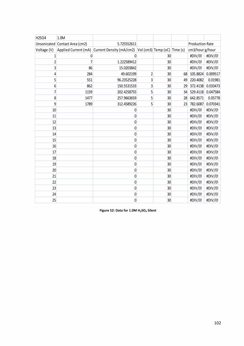
102
H2SO4 1.0M
Unsonicated Contact Area (cm2) 5.725552611 Production Rate
Voltage (V) Applied Current (mA) Current Density (mA/cm2) Vol (cm3) Temp (oC) Time (s) cm3/hour g/hour
1 0 0 30 #DIV/0! #DIV/0!
2 7 1.222589412 30 #DIV/0! #DIV/0!
3 86 15.0203842 30 #DIV/0! #DIV/0!
4 284 49.602199 2 30 68 105.8824 0.009517
5 551 96.23525228 3 30 49 220.4082 0.01981
6 862 150.5531533 3 30 29 372.4138 0.033473
7 1159 202.4258755 5 30 34 529.4118 0.047584
8 1477 257.9663659 5 30 28 642.8571 0.05778
9 1789 312.4589226 5 30 23 782.6087 0.070341
10 0 30 #DIV/0! #DIV/0!
11 0 30 #DIV/0! #DIV/0!
12 0 30 #DIV/0! #DIV/0!
13 0 30 #DIV/0! #DIV/0!
14 0 30 #DIV/0! #DIV/0!
15 0 30 #DIV/0! #DIV/0!
16 0 30 #DIV/0! #DIV/0!
17 0 30 #DIV/0! #DIV/0!
18 0 30 #DIV/0! #DIV/0!
19 0 30 #DIV/0! #DIV/0!
20 0 30 #DIV/0! #DIV/0!
21 0 30 #DIV/0! #DIV/0!
22 0 30 #DIV/0! #DIV/0!
23 0 30 #DIV/0! #DIV/0!
24 0 30 #DIV/0! #DIV/0!
25 0 30 #DIV/0! #DIV/0!
Figure 52: Data for 1.0M H2SO4 Silent

103
H2SO4
Unsonicated 0.1M 0.2M 0.3M 0.4M 0.5M 1.0M
Voltage (V) V ideal Efficiency (%) V ideal Efficiency (%) V ideal Efficiency (%) V ideal Efficiency (%) V ideal Efficiency (%) V ideal Efficiency (%)
1 0 #DIV/0! 0 #DIV/0! 0 #DIV/0! 0 #DIV/0! 0 #DIV/0! 0 #DIV/0!
2 0 #DIV/0! 0 #DIV/0! 0 #DIV/0! 0 #DIV/0! 0 #DIV/0! 0 #DIV/0!
3 0 #DIV/0! 0 #DIV/0! 0 #DIV/0! 0 #DIV/0! 0 #DIV/0! 0 #DIV/0!
4 0 #DIV/0! 0 #DIV/0! 1.961393 50.98418552 2.632508 37.98659103 3.390125 29.49743566 4.405408 45.39874985
5 0 #DIV/0! 3.355 29.80625717 2.517704 39.71872557 4.457887 44.86430293 4.061352 49.24468669 6.158948 48.70961835
6 4.008596 24.94639047 2.380792 42.002821 1.96723 50.83289714 3.80409 52.57499643 6.700483 44.77289341 5.702484 52.60864812
7 3.32386 30.08550463 2.991287 33.43042708 3.681503 54.32564377 5.14885 58.26543858 6.69935 44.78046586 8.989203 55.62228196
8 2.97867 33.57202705 5.347605 37.39991842 5.23038 57.35720872 5.068487 59.18925715 8.086672 49.46410396 9.434033 52.99960448
9 2.320981 43.0852272 4.73847 42.20771281 5.23038 57.35720872 6.435235 62.15778787 9.552176 52.3440925 9.386356 53.268808
10 2.258909 44.26915239 4.341898 46.0628014 6.476098 61.76558982 8.703679 57.44696961 9.625599 51.9448203 0 #DIV/0!
11 2.312809 43.23747182 5.917309 50.69871754 6.95049 57.54989811 7.371567 67.82818473 10.40968 48.03222281 0 #DIV/0!
12 2.289459 43.67844553 6.302098 47.60319713 6.655503 60.10064204 7.588721 65.88725514 9.89844 50.51300795 0 #DIV/0!
13 2.123285 47.09682827 6.373707 47.06836778 7.83156 63.84423948 7.575879 65.99894566 9.603844 52.06248672 0 #DIV/0!
14 3.642586 54.90604595 6.16749 48.6421558 8.150676 61.34460825 7.802762 64.07987408 9.767912 51.18801473 0 #DIV/0!
15 3.80409 52.57499643 6.519646 46.01476928 7.927295 63.07321921 7.78272 64.24489213 10.26782 48.69583287 0 #DIV/0!
16 3.92979 50.89330462 6.700483 44.77289341 9.897249 60.62290698 8.386121 59.62232471 0 #DIV/0! 0 #DIV/0!
17 3.756222 53.24498447 6.161145 48.69225071 8.06934 61.96293587 0 #DIV/0! 0 #DIV/0! 0 #DIV/0!
18 3.650369 54.78897549 8.320083 48.0764415 8.107089 61.67441797 0 #DIV/0! 0 #DIV/0! 0 #DIV/0!
19 3.54296 56.44997694 8.521542 46.93986144 7.855299 63.65129924 0 #DIV/0! 0 #DIV/0! 0 #DIV/0!
20 3.442166 58.1029497 8.622158 46.39209813 7.927295 63.07321921 0 #DIV/0! 0 #DIV/0! 0 #DIV/0!
21 3.283387 60.91271662 8.774215 45.58812339 0 #DIV/0! 0 #DIV/0! 0 #DIV/0! 0 #DIV/0!
22 5.269297 56.93359565 7.529205 53.12645748 0 #DIV/0! 0 #DIV/0! 0 #DIV/0! 0 #DIV/0!
23 4.903481 61.18102263 7.619624 52.4960311 0 #DIV/0! 0 #DIV/0! 0 #DIV/0! 0 #DIV/0!
24 4.880131 61.4737548 7.635713 52.38541474 0 #DIV/0! 0 #DIV/0! 0 #DIV/0! 0 #DIV/0!
25 8.044044 49.72623029 9.008759 55.50153914 0 #DIV/0! 0 #DIV/0! 0 #DIV/0! 0 #DIV/0!
Figure 53: Data of H2SO4 Efficiency of H2 production

104
Sonicated
NaOH 0.1M
Sonicated Contact Area (cm2) 6.668030407 Production Rate
Voltage (V) Applied Current (mA) Current Density (mA/cm2) Vol (cm3) Temp (oC) Time (s) cm3/hour g/hour
1 0 0 0 #DIV/0! #DIV/0!
2 3 0.449907966 0 #DIV/0! #DIV/0!
3 17 2.549478476 0 #DIV/0! #DIV/0!
4 35 5.248926274 0 #DIV/0! #DIV/0!
5 54 8.098343394 0 #DIV/0! #DIV/0!
6 74 11.09772984 0 24.8 #DIV/0! #DIV/0!
7 98 14.69699357 1 24.5 188 19.14894 0.001721
8 115 17.24647204 1 24.6 146 24.65753 0.002216
9 134 20.09588916 1 24.7 112 32.14286 0.002889
10 154 23.09527561 1 24.6 91 39.56044 0.003556
11 171 25.64475408 1 24.6 85 42.35294 0.003807
12 189 28.34420188 1 24.6 65 55.38462 0.004978
13 208 31.193619 1 24.5 59 61.01695 0.005484
14 226 33.8930668 1 24.6 53 67.92453 0.006105
15 247 37.04242256 1 24.7 42 85.71429 0.007704
16 266 39.89183968 1 25.6 39 92.30769 0.008297
17 294 44.0909807 2 24.5 68 105.8824 0.009517
18 314 47.09036714 2 24.5 60 120 0.010786
19 337 50.53966155 2 24.2 58 124.1379 0.011158
20 357 53.53904799 2 24.2 54 133.3333 0.011984
21 372 55.78858783 2 24.2 53 135.8491 0.01221
22 392 58.78797427 2 24 50 144 0.012943
23 410 61.48742207 2 24.6 47 153.1915 0.013769
24 430 64.48680851 2 24.5 42 171.4286 0.015408
25 444 66.58637902 3 24.3 57 189.4737 0.01703
Figure 54: Data for 0.1M NaOH Sonicated

105
NaOH 0.2M
Sonicated Contact Area (cm2) 4.783074815 Production Rate
Voltage (V) Applied Current (mA) Current Density (mA/cm2) Vol (cm3) Temp (oC) Time (s) cm3/hour g/hour
1 0 0 0 #DIV/0! #DIV/0!
2 5 1.045352664 0 #DIV/0! #DIV/0!
3 31 6.481186517 0 #DIV/0! #DIV/0!
4 69 14.42586676 0 #DIV/0! #DIV/0!
5 107 22.37054701 1 26.8 112 32.14286 0.002889
6 147 30.73336832 1 26.8 96 37.5 0.003371
7 187 39.09618963 1 26.8 80 45 0.004045
8 227 47.45901094 1 26.9 54 66.66667 0.005992
9 266 55.61276172 1 27 42 85.71429 0.007704
10 309 64.60279463 1 27.4 34 105.8824 0.009517
11 354 74.01096861 2 27.3 57 126.3158 0.011353
12 400 83.62821312 2 27.4 49 146.9388 0.013207
13 438 91.57289337 2 27.4 42 171.4286 0.015408
14 494 103.2808432 2 27.5 36 200 0.017976
15 521 108.9257476 3 27.5 54 200 0.017976
16 564 117.9157805 3 27.5 48 225 0.020223
17 606 126.6967429 3 27.5 45 240 0.021571
18 650 135.8958463 4 27.5 65 221.5385 0.019912
19 686 143.4223855 4 28 50 288 0.025885
20 745 155.7575469 4 27.3 46 313.0435 0.028136
21 777 162.447804 4 27.3 42 342.8571 0.030816
22 831 173.7376128 4 27.5 42 342.8571 0.030816
23 856 178.9643761 4 27.1 37 389.1892 0.03498
24 896 187.3271974 4 27.1 49 293.8776 0.026414
25 930 194.4355955 5 27 48 375 0.033705
Figure 55: Data for 0.2M NaOH Sonicated

106
NaOH 0.3M
Sonicated Contact Area (cm2) 4.783074815 Production Rate
Voltage (V) Applied Current (mA) Current Density (mA/cm2) Vol (cm3) Temp (oC) Time (s) cm3/hour g/hour
1 0 0 #DIV/0! #DIV/0!
2 5 1.045352664 #DIV/0! #DIV/0!
3 33 6.899327582 #DIV/0! #DIV/0!
4 75 15.68028996 #DIV/0! #DIV/0!
5 118 24.67032287 #DIV/0! #DIV/0!
6 162 33.86942631 1 27.3 110 32.72727 0.002942
7 206 43.06852976 1 27.2 78 46.15385 0.004148
8 250 52.2676332 1 27.2 57 63.15789 0.005677
9 297 62.09394824 1 27.1 51 70.58824 0.006344
10 343 71.71119275 1 27.4 48 75 0.006741
11 388 81.11936673 1 27.3 46 78.26087 0.007034
12 440 91.99103443 2 27.9 50 144 0.012943
13 485 101.3992084 2 27.9 38 189.4737 0.01703
14 533 111.434594 2 27.9 36 200 0.017976
15 578 120.842768 3 28 51 211.7647 0.019033
16 628 131.2962946 3 28 46 234.7826 0.021102
17 676 141.3316802 3 28 42 257.1429 0.023112
18 719 150.3217131 3 27.9 39 276.9231 0.02489
19 769 160.7752397 3 28.1 38 284.2105 0.025545
20 820 171.4378369 4 27.8 47 306.383 0.027538
21 862 180.2187993 4 27.8 45 320 0.028762
22 908 189.8360438 4 27.9 40 360 0.032357
23 956 199.8714294 4 27.8 36 400 0.035952
24 1005 210.1158855 4 28 34 423.5294 0.038067
25 1059 221.4056942 5 27.6 43 418.6047 0.037624
Figure 56: Data for 0.3M NaOH Sonicated

107
NaOH 0.4M
Sonicated Contact Area (cm2) 5.725552611 Production Rate
Voltage (V) Applied Current (mA) Current Density (mA/cm2) Vol (cm3) Temp (oC) Time (s) cm3/hour g/hour
1 0 0 #DIV/0! #DIV/0!
2 4 0.698622521 #DIV/0! #DIV/0!
3 44 7.684847732 #DIV/0! #DIV/0!
4 98 17.11625177 #DIV/0! #DIV/0!
5 155 27.07162269 1 25.8 88 40.90909 0.003677
6 213 37.20164925 1 25.8 68 52.94118 0.004758
7 272 47.50633144 1 25.8 51 70.58824 0.006344
8 330 57.63635799 1 25.8 34 105.8824 0.009517
9 387 67.59172892 2 25.9 57 126.3158 0.011353
10 448 78.24572237 2 25.8 48 150 0.013482
11 508 88.72506018 2 25.8 38 189.4737 0.01703
12 568 99.204398 2 26 34 211.7647 0.019033
13 628 109.6837358 3 26.4 47 229.7872 0.020653
14 687 119.988418 3 26.2 41 263.4146 0.023676
15 748 130.6424114 3 25.9 34 317.6471 0.02855
16 805 140.5977824 4 25.8 47 306.383 0.027538
17 859 150.0291864 4 25.9 43 334.8837 0.030099
18 925 161.556458 4 25.8 38 378.9474 0.03406
19 984 171.8611402 4 26.6 37 389.1892 0.03498
20 1053 183.9123787 5 26.6 42 428.5714 0.03852
21 1099 191.9465377 5 25.6 40 450 0.040446
22 1163 203.124498 5 25.8 38 473.6842 0.042575
23 1233 215.3503921 5 25.3 36 500 0.04494
24 1269 221.6379948 5 25.1 35 514.2857 0.046224
25 1328 231.942677 5 25.3 34 529.4118 0.047584
Figure 57: Data for 0.4M NaOH Sonicated

108
NaOH 0.5M
Sonicated Contact Area (cm2) 5.725552611 Production Rate
Voltage (V) Applied Current (mA) Current Density (mA/cm2) Vol (cm3) Temp (oC) Time (s) cm3/hour g/hour
1 0 0 #DIV/0! #DIV/0!
2 6 1.047933782 #DIV/0! #DIV/0!
3 53 9.256748405 #DIV/0! #DIV/0!
4 184 32.13663597 1 27 89 40.44944 0.003636
5 199 34.75647043 1 27 65 55.38462 0.004978
6 271 47.33167581 1 27 43 83.72093 0.007525
7 354 61.82809312 1 27 30 120 0.010786
8 428 74.75260976 2 27.1 48 150 0.013482
9 505 88.20109329 2 27.2 38 189.4737 0.01703
10 582 101.6495768 3 27.1 49 220.4082 0.01981
11 658 114.9234047 3 27.1 47 229.7872 0.020653
12 750 130.9917227 4 27.2 47 306.383 0.027538
13 828 144.6148619 5 27.4 54 333.3333 0.02996
14 915 159.8099017 5 27.5 48 375 0.033705
15 990 172.909074 5 27.4 43 418.6047 0.037624
16 1073 187.4054913 5 27.1 42 428.5714 0.03852
17 1161 202.7751868 5 27.5 37 486.4865 0.043725
18 1241 216.7476372 5 27.8 34 529.4118 0.047584
19 1309 228.62422 5 26.5 33 545.4545 0.049025
20 1350 235.7851009 5 26.3 27 666.6667 0.05992
21 1467 256.2198096 5 25.8 25 720 0.064714
22 1554 271.4148495 5 25.8 23 782.6087 0.070341
23 0 #DIV/0! #DIV/0!
24 0 #DIV/0! #DIV/0!
25 0 #DIV/0! #DIV/0!
Figure 58: Data for 0.5M NaOH Sonicated

109
NaOH 1.0M
Sonicated Contact Area (cm2) 5.725552611 Production Rate
Voltage (V) Applied Current (mA) Current Density (mA/cm2) Vol (cm3) Temp (oC) Time (s) cm3/hour g/hour
1 0 0 #DIV/0! #DIV/0!
2 6 1.047933782 #DIV/0! #DIV/0!
3 95 16.59228488 #DIV/0! #DIV/0!
4 216 37.72561614 1 27.4 55 65.45455 0.005883
5 346 60.43084808 1 27.5 31 116.129 0.010438
6 477 83.31073564 3 27.5 57 189.4737 0.01703
7 611 106.7145901 3 27.5 53 203.7736 0.018315
8 751 131.1663783 4 27.7 47 306.383 0.027538
9 872 152.2997096 4 28 42 342.8571 0.030816
10 1023 178.6727098 5 28 40 450 0.040446
11 1157 202.0765642 5 28.2 36 500 0.04494
12 1261 220.2407498 5 27.9 32 562.5 0.050558
13 1395 243.6446042 5 28.3 30 600 0.053928
14 1490 260.2368891 5 28.2 29 620.6897 0.055788
15 1622 283.2914323 5 28.3 24 750 0.06741
16 1796 313.681512 5 28.3 22 818.1818 0.073538
17 1840 321.3663597 5 28.1 21 857.1429 0.07704
18 0 #DIV/0! #DIV/0!
19 0 #DIV/0! #DIV/0!
20 0 #DIV/0! #DIV/0!
21 0 #DIV/0! #DIV/0!
22 0 #DIV/0! #DIV/0!
23 0 #DIV/0! #DIV/0!
24 0 #DIV/0! #DIV/0!
25 0 #DIV/0! #DIV/0!
Figure 59: Data for 1.0M NaOH Sonicated

110
NaOH
Sonicated 0.1M 0.2M 0.3M 0.4M 0.5M 1.0M
Voltage (V) V ideal Efficiency (%) V ideal Efficiency (%) V ideal Efficiency (%) V ideal Efficiency (%) V ideal Efficiency (%) V ideal Efficiency (%)
1 0 #DIV/0! 0 #DIV/0! 0 #DIV/0! 0 #DIV/0! 0 #DIV/0! 0 #DIV/0!
2 0 #DIV/0! 0 #DIV/0! 0 #DIV/0! 0 #DIV/0! 0 #DIV/0! 0 #DIV/0!
3 0 #DIV/0! 0 #DIV/0! 0 #DIV/0! 0 #DIV/0! 0 #DIV/0! 0 #DIV/0!
4 0 #DIV/0! 0 #DIV/0! 0 #DIV/0! 0 #DIV/0! 3.698686 27.03662928 2.686794 37.21907
5 0 #DIV/0! 3.237891 30.88430418 0 #DIV/0! 3.068416 32.59010768 2.921501 34.22897883 2.426612 41.20973
6 0 #DIV/0! 3.812843 26.2271472 4.822713 20.73521676 3.25828 30.69104314 2.631948 37.99466585 6.151142 48.77144
7 3.543324 28.22208357 4.04196 24.74047469 4.347113 23.00377062 3.120606 32.04505974 2.398635 41.69038052 7.326213 40.94885
8 3.230157 30.95825115 3.313025 30.1838921 3.855263 25.93856746 2.524019 39.61934659 4.641617 43.08843264 7.990778 50.0577
9 2.888295 34.62250287 3.020514 33.10695306 4.096577 24.41062204 4.96399 40.29016925 4.337144 46.11328996 8.299462 48.1959
10 2.696094 37.09069764 2.844236 35.15882552 4.457215 22.43553334 4.837479 41.3438494 6.443226 46.56052809 9.27299 53.92004
11 2.796327 35.76119964 5.46087 36.62420088 4.830291 20.70268729 4.342573 46.05564326 6.987278 42.93517235 9.445139 52.93729
12 2.363459 42.31086991 5.306209 37.69169601 5.965857 33.52410337 4.347279 46.00578646 7.966876 50.20788847 9.141237 54.69719
13 2.360165 42.36992077 4.980256 40.15858023 4.997761 40.01792046 6.653162 45.09134114 10.11212 49.4456282 9.493187 52.66935
14 2.304396 43.39531114 4.816174 41.52673874 5.203312 38.43705827 6.344847 47.28246633 9.936303 50.32052786 9.798436 51.02855
15 1.99648 50.0881553 7.619109 39.37468127 7.996361 37.51706541 5.723024 52.41983584 9.62768 51.93359004 8.830365 56.6228
16 2.002513 49.93726211 7.331504 40.91929975 7.836314 38.2833029 8.511254 46.99659773 10.182 49.10624196 8.962839 55.7859
17 3.844884 52.01717364 7.385125 40.62219592 7.701767 38.95210109 8.312022 48.12306595 9.718437 51.44860171 8.75922 57.08271
18 3.62333 55.19784159 11.44193 34.95912529 7.604027 39.45278026 7.907244 50.58652276 9.555344 52.32674036 0 #DIV/0!
19 3.75532 53.2577781 9.304403 42.99040056 7.929549 37.83317163 8.212158 48.70826953 9.740228 51.33349802 0 #DIV/0!
20 3.70383 53.99816012 9.274656 43.12828278 10.44762 38.28621388 9.975579 50.1224019 8.213403 60.87610785 0 #DIV/0!
21 3.787982 52.79856618 8.831898 45.29037969 10.5154 38.03946076 9.882501 50.59447924 8.250304 60.60382669 0 #DIV/0!
22 3.763162 53.14679445 9.451985 42.31915201 9.849087 40.61290056 9.941757 50.29292085 8.040419 62.18581344 0 #DIV/0!
23 3.707273 53.94800589 8.565841 46.69710684 9.329669 42.87397382 9.968698 50.1570017 0 #DIV/0! 0 #DIV/0!
24 3.47332 57.58180152 11.87404 33.68692529 9.269138 43.15395783 9.968077 50.16012488 0 #DIV/0! 0 #DIV/0!
25 4.863993 61.67772427 12.06908 41.42818992 12.3362 40.53110466 10.14028 49.30831395 0 #DIV/0! 0 #DIV/0!
Figure 60: Data of NaOH Efficiency of H2 production

111
NaCl 0.1M
Sonicated Contact Area (cm2) 6.668030407 Production Rate
Voltage (V) Applied Current (mA) Current Density (mA/cm2) Vol (cm3) Temp (oC) Time (s) cm3/hour g/hour
1 0 0 #DIV/0! #DIV/0!
2 0 0 #DIV/0! #DIV/0!
3 0 0 #DIV/0! #DIV/0!
4 0 0 #DIV/0! #DIV/0!
5 0 0 #DIV/0! #DIV/0!
6 2 0.299938644 #DIV/0! #DIV/0!
7 5 0.749846611 #DIV/0! #DIV/0!
8 17 2.549478476 #DIV/0! #DIV/0!
9 35 5.248926274 #DIV/0! #DIV/0!
10 44 6.598650173 #DIV/0! #DIV/0!
11 55 8.248312716 #DIV/0! #DIV/0!
12 68 10.1979139 #DIV/0! #DIV/0!
13 81 12.14751509 #DIV/0! #DIV/0!
14 93 13.94714696 #DIV/0! #DIV/0!
15 104 15.5968095 #DIV/0! #DIV/0!
16 116 17.39644137 1 26.2 123 29.26829 0.002631
17 128 19.19607323 1 26 113 31.85841 0.002863
18 138 20.69576645 1 25.5 106 33.96226 0.003053
19 149 22.34542899 1 25.6 103 34.95146 0.003141
20 157 23.54518357 1 25.5 95 37.89474 0.003406
21 167 25.04487679 1 25.1 89 40.44944 0.003636
22 176 26.39460069 1 25.1 74 48.64865 0.004373
23 186 27.89429391 1 25 72 50 0.004494
24 193 28.94407917 1 24.9 67 53.73134 0.004829
25 202 30.29380307 1 24.8 61 59.01639 0.005304
Figure 61: Data for 0.1M NaCl Sonicated

112
NaCl 0.2M
Sonicated Contact Area (cm2) 6.668030407 Production Rate
Voltage (V) Applied Current (mA) Current Density (mA/cm2) Vol (cm3) Temp (oC) Time (s) cm3/hour g/hour
1 0 0 #DIV/0! #DIV/0!
2 2 0.299938644 #DIV/0! #DIV/0!
3 6 0.899815933 #DIV/0! #DIV/0!
4 20 2.999386442 #DIV/0! #DIV/0!
5 37 5.548864918 #DIV/0! #DIV/0!
6 55 8.248312716 #DIV/0! #DIV/0!
7 74 11.09772984 #DIV/0! #DIV/0!
8 93 13.94714696 #DIV/0! #DIV/0!
9 112 16.79656408 #DIV/0! #DIV/0!
10 131 19.6459812 1 26.2 137 26.27737 0.002362
11 150 22.49539832 1 26.2 112 32.14286 0.002889
12 173 25.94469273 1 26.2 96 37.5 0.003371
13 189 28.34420188 1 26.3 81 44.44444 0.003995
14 205 30.74371103 1 26.6 72 50 0.004494
15 233 34.94285205 1 26.1 58 62.06897 0.005579
16 252 37.79226917 1 26.3 49 73.46939 0.006603
17 268 40.19177833 1 25.8 43 83.72093 0.007525
18 286 42.89122612 1 26 42 85.71429 0.007704
19 308 46.19055121 1 25.7 41 87.80488 0.007892
20 325 48.74002969 1 25.5 40 90 0.008089
21 346 51.88938545 2 26.3 62 116.129 0.010438
22 362 54.2888946 2 26 55 130.9091 0.011766
23 382 57.28828105 2 25.8 53 135.8491 0.01221
24 405 60.73757546 2 25.5 49 146.9388 0.013207
25 424 63.58699258 2 27.6 48 150 0.013482
Figure 62: Data for 0.2M NaCl Sonicated

113
NaCl 0.3M
Sonicated Contact Area (cm2) 4.783074815 Production Rate
Voltage (V) Applied Current (mA) Current Density (mA/cm2) Vol (cm3) Temp (oC) Time (s) cm3/hour g/hour
1 0 0 #DIV/0! #DIV/0!
2 1 0.209070533 #DIV/0! #DIV/0!
3 8 1.672564262 #DIV/0! #DIV/0!
4 28 5.853974918 #DIV/0! #DIV/0!
5 53 11.08073824 #DIV/0! #DIV/0!
6 79 16.51657209 #DIV/0! #DIV/0!
7 105 21.95240594 #DIV/0! #DIV/0!
8 134 28.01545139 1 27.3 120 30 0.002696
9 160 33.45128525 1 27.5 95 37.89474 0.003406
10 190 39.72340123 1 27.5 70 51.42857 0.004622
11 221 46.20458775 1 27.5 57 63.15789 0.005677
12 249 52.05856267 1 27.6 56 64.28571 0.005778
13 280 58.53974918 1 27.5 46 78.26087 0.007034
14 308 64.3937241 1 27.7 45 80 0.00719
15 340 71.08398115 1 27.8 43 83.72093 0.007525
16 372 77.7742382 1 27.8 32 112.5 0.010112
17 400 83.62821312 1 27.9 31 116.129 0.010438
18 435 90.94568177 1 27.9 26 138.4615 0.012445
19 476 99.51757361 2 28.1 48 150 0.013482
20 488 102.02642 2 27.7 42 171.4286 0.015408
21 519 108.5076065 2 27.5 39 184.6154 0.016593
22 549 114.7797225 2 27.7 37 194.5946 0.01749
23 579 121.0518385 2 27.5 35 205.7143 0.01849
24 609 127.3239545 2 27.4 32 225 0.020223
25 646 135.0595642 2 27.3 30 240 0.021571
Figure 63: Data for 0.3M NaCl Sonicated

114
NaCl 0.4M
Sonicated Contact Area (cm2) 5.725552611 Production Rate
Voltage (V) Applied Current (mA) Current Density (mA/cm2) Vol (cm3) Temp (oC) Time (s) cm3/hour g/hour
1 0 #DIV/0! #DIV/0!
2 1 0.17465563 #DIV/0! #DIV/0!
3 9 1.571900673 #DIV/0! #DIV/0!
4 37 6.46225832 #DIV/0! #DIV/0!
5 70 12.22589412 #DIV/0! #DIV/0!
6 103 17.98952992 #DIV/0! #DIV/0!
7 139 24.27713261 1 26.8 139 25.89928 0.002328
8 178 31.08870219 1 26.8 92 39.13043 0.003517
9 215 37.55096051 1 26.9 66 54.54545 0.004903
10 257 44.88649698 1 27 51 70.58824 0.006344
11 296 51.69806656 1 27.5 48 75 0.006741
12 330 57.63635799 1 27.6 39 92.30769 0.008297
13 369 64.44792757 1 27.8 28 128.5714 0.011556
14 409 71.43415278 2 27.8 52 138.4615 0.012445
15 450 78.59503363 2 28 45 160 0.014381
16 485 84.70798069 2 28.1 39 184.6154 0.016593
17 531 92.74213968 2 28 38 189.4737 0.01703
18 569 99.37905363 2 28.2 37 194.5946 0.01749
19 614 107.238557 2 28.3 35 205.7143 0.01849
20 659 115.0980604 2 28.4 29 248.2759 0.022315
21 690 120.5123849 3 27.9 43 251.1628 0.022575
22 725 126.625332 3 27.9 41 263.4146 0.023676
23 762 133.0875903 3 28.3 34 317.6471 0.02855
24 808 141.1217493 4 28.2 45 320 0.028762
25 844 147.409352 4 28.2 42 342.8571 0.030816
Figure 64: Data for 0.4M NaCl Sonicated

115
NaCl 0.5M
Sonicated Contact Area (cm2) 5.254313713 Production Rate
Voltage (V) Applied Current (mA) Current Density (mA/cm2) Vol (cm3) Temp (oC) Time (s) cm3/hour g/hour
1 0 0 #DIV/0! #DIV/0!
2 2 0.380639625 #DIV/0! #DIV/0!
3 13 2.474157561 #DIV/0! #DIV/0!
4 43 8.183751932 #DIV/0! #DIV/0!
5 78 14.84494536 #DIV/0! #DIV/0!
6 115 21.88677842 #DIV/0! #DIV/0!
7 154 29.3092511 1 27.6 203 17.73399 0.001594
8 190 36.16076435 1 27.5 105 34.28571 0.003082
9 232 44.15419647 1 27.6 84 42.85714 0.003852
10 271 51.57666915 1 27.8 67 53.73134 0.004829
11 316 60.14106071 1 27.8 45 80 0.00719
12 353 67.18289377 1 27.9 39 92.30769 0.008297
13 398 75.74728532 1 28.3 32 112.5 0.010112
14 443 84.31167688 2 28.3 52 138.4615 0.012445
15 486 92.49542881 2 28.4 43 167.4419 0.01505
16 526 100.1082213 2 28.6 39 184.6154 0.016593
17 571 108.6726129 2 28.8 37 194.5946 0.01749
18 625 118.9498827 3 29 48 225 0.020223
19 658 125.2304365 3 28.8 42 257.1429 0.023112
20 702 133.6045083 3 28.8 39 276.9231 0.02489
21 748 142.3592197 3 28.8 36 300 0.026964
22 792 150.7332914 3 29.9 35 308.5714 0.027734
23 833 158.5364037 4 28.9 45 320 0.028762
24 884 168.2427141 4 28.7 44 327.2727 0.029415
25 948 180.4231821 4 29.3 41 351.2195 0.031568
Figure 65: Data for 0.5M NaCl Sonicated

116
NaCl 1.0M
Sonicated Contact Area (cm2) 6.668030407 Production Rate
Voltage (V) Applied Current (mA) Current Density (mA/cm2) Vol (cm3) Temp (oC) Time (s) cm3/hour g/hour
1 1 0.149969322 #DIV/0! #DIV/0!
2 5 0.749846611 #DIV/0! #DIV/0!
3 21 3.149355764 #DIV/0! #DIV/0!
4 73 10.94776051 #DIV/0! #DIV/0!
5 143 21.44561306 1 27.7 134 26.86567 0.002415
6 218 32.69331222 1 27.7 76 47.36842 0.004257
7 294 44.0909807 1 28 46 78.26087 0.007034
8 372 55.78858783 1 28.1 40 90 0.008089
9 444 66.58637902 1 28.2 44 81.81818 0.007354
10 520 77.9840475 2 28.3 40 180 0.016178
11 609 91.33131717 2 28.4 32 225 0.020223
12 696 104.3786482 3 28.5 40 270 0.024268
13 772 115.7763167 4 28.7 51 282.3529 0.025378
14 845 126.7240772 5 28.9 52 346.1538 0.031112
15 942 141.2711014 5 28.9 45 400 0.035952
16 1025 153.7185552 5 29 42 428.5714 0.03852
17 1108 166.1660089 5 29.1 37 486.4865 0.043725
18 1180 176.9638001 5 28.8 35 514.2857 0.046224
19 1260 188.9613459 5 28.9 33 545.4545 0.049025
20 1343 201.4087996 5 29 32 562.5 0.050558
21 1447 217.0056091 5 28.9 29 620.6897 0.055788
22 1510 226.4536764 5 28.5 28 642.8571 0.05778
23 1582 237.2514676 5 28.8 28 642.8571 0.05778
24 1673 250.8986759 5 28.5 27 666.6667 0.05992
25 1714 257.0474181 5 28 26 692.3077 0.062225
Figure 66: Data for 1.0M NaCl Sonicated

117
NaCl
Sonicated 0.1M 0.2M 0.3M 0.4M 0.5M 1.0M
Voltage (V) V ideal Efficiency (%) V ideal Efficiency (%) V ideal Efficiency (%) V ideal Efficiency (%) V ideal Efficiency (%) V ideal Efficiency (%)
1 0 #DIV/0! 0 #DIV/0! 0 #DIV/0! 0 #DIV/0! 0 #DIV/0! 0 #DIV/0!
2 0 #DIV/0! 0 #DIV/0! 0 #DIV/0! 0 #DIV/0! 0 #DIV/0! 0 #DIV/0!
3 0 #DIV/0! 0 #DIV/0! 0 #DIV/0! 0 #DIV/0! 0 #DIV/0! 0 #DIV/0!
4 0 #DIV/0! 0 #DIV/0! 0 #DIV/0! 0 #DIV/0! 0 #DIV/0! 0 #DIV/0!
5 0 #DIV/0! 0 #DIV/0! 0 #DIV/0! 0 #DIV/0! 0 #DIV/0! 3.724877 26.84652221
6 0 #DIV/0! 0 #DIV/0! 0 #DIV/0! 0 #DIV/0! 0 #DIV/0! 3.220633 31.04979833
7 0 #DIV/0! 0 #DIV/0! 0 #DIV/0! 4.360936 22.93085545 7.70948 12.97104357 2.631535 38.00063517
8 0 #DIV/0! 0 #DIV/0! 4.351808 22.9789529 3.696221 27.05465671 4.918207 20.33261348 2.89635 34.52620928
9 0 #DIV/0! 0 #DIV/0! 4.116388 24.29314216 3.203888 31.21207896 4.80591 20.80771573 3.80389 26.28887752
10 0 #DIV/0! 3.471301 28.80764524 3.60184 27.76359105 2.960349 33.77980019 4.480651 22.31818492 4.05135 49.36626361
11 0 #DIV/0! 3.249449 30.77445292 3.411457 29.31299205 3.214367 31.11032635 3.509107 28.49727733 3.797062 52.67229934
12 0 #DIV/0! 3.212312 31.13022695 3.7775 26.47253174 2.912631 34.33322033 3.398448 29.42519632 5.426173 55.28757984
13 0 #DIV/0! 2.962049 33.76041254 3.488097 28.66892554 2.339807 42.73856916 3.148118 31.76500839 7.678913 52.09070319
14 0 #DIV/0! 2.858687 34.98108987 3.755993 26.62411875 4.816397 41.5248163 5.694099 35.12407943 8.575511 58.30556352
15 0 #DIV/0! 2.612999 38.27020704 3.963266 25.23171483 4.588906 43.5833716 5.167337 38.70465948 8.273007 60.43751972
16 2.75971 36.23568889 2.389142 41.85602167 3.226999 30.98854761 4.287802 46.64394966 5.075751 39.40303538 8.404597 59.49125564
17 2.795751 35.76856072 2.225989 44.92386134 3.362574 29.73912396 4.57259 43.73888764 5.23089 38.23441435 8.006246 62.45124429
18 2.822725 35.42675833 2.321803 43.06996856 3.066993 32.60522874 4.774044 41.89319979 7.432699 40.36218925 8.057609 62.05314596
19 2.96246 33.75572797 2.438422 41.01012113 6.19993 32.25843083 4.874757 41.02768529 6.84247 43.84381633 8.114924 61.614874
20 2.878107 34.74506341 2.508574 39.86327852 5.554317 36.00802946 4.336547 46.11964693 6.778591 44.256984 8.39015 59.59369312
21 2.864231 34.91338482 4.150622 48.185545 5.481566 36.48592075 6.721365 44.63379356 6.667174 44.99657264 8.189672 61.05250961
22 2.50984 39.84318478 3.84841 51.96950902 5.504725 36.33242612 6.733824 44.5512079 6.888271 43.55229582 8.240611 60.67511127
23 2.579891 38.76132649 3.91074 51.14122079 5.488066 36.44271018 5.876929 51.0470679 9.284084 43.08448926 8.642127 57.85612534
24 2.490247 40.15666592 3.829435 52.2270215 5.275887 37.90831495 8.245108 48.5136158 9.627174 41.54905807 8.804083 56.79182893
25 2.372169 42.15550451 3.954885 50.57037232 5.244903 38.13225621 8.0383 49.76176569 9.639366 41.49650511 8.671379 57.66095841
Figure 67: Data of NaCl Efficiency of H2 production

118
H2SO4 0.1M
Sonicated Contact Area (cm2) 4.783074815 Production Rate
Voltage (V) Applied Current (mA) Current Density (mA/cm2) Vol (cm3) Temp (oC) Time (s) cm3/hour g/hour
1 0 0 #DIV/0! #DIV/0!
2 2 0.418141066 #DIV/0! #DIV/0!
3 23 4.808622254 #DIV/0! #DIV/0!
4 59 12.33516144 #DIV/0! #DIV/0!
5 97 20.27984168 #DIV/0! #DIV/0!
6 135 28.22452193 1 27.9 104 34.61538 0.003111
7 175 36.58734324 1 28.2 71 50.70423 0.004557
8 215 44.95016455 1 28 56 64.28571 0.005778
9 256 53.5220564 1 28 50 72 0.006471
10 302 63.1393009 1 28.2 38 94.73684 0.008515
11 337 70.45676955 1 28.5 33 109.0909 0.009805
12 378 79.0286614 2 28.3 51 141.1765 0.012689
13 420 87.80962377 2 28.3 44 163.6364 0.014708
14 458 95.75430402 2 29.1 39 184.6154 0.016593
15 502 104.9534075 2 29.3 38 189.4737 0.01703
16 542 113.3162288 2 29.2 35 205.7143 0.01849
17 585 122.3062617 3 29.3 48 225 0.020223
18 622 130.0418714 3 29.5 44 245.4545 0.022061
19 661 138.1956222 3 29.5 40 270 0.024268
20 709 148.2310078 4 29.7 48 300 0.026964
21 764 159.7298871 4 29.2 45 320 0.028762
22 793 165.7929325 4 30 44 327.2727 0.029415
23 835 174.5738949 4 29.5 43 334.8837 0.030099
24 885 185.0274215 4 28.8 39 369.2308 0.033186
25 919 192.1358196 4 30.2 35 411.4286 0.036979
Figure 68: Data for 0.1M H2SO4 Sonicated

119
H2SO4 0.2M
Sonicated Contact Area (cm2) 6.668030407 Production Rate
Voltage (V) Applied Current (mA) Current Density (mA/cm2) Vol (cm3) Temp (oC) Time (s) cm3/hour g/hour
1 0 #DIV/0! #DIV/0!
2 1 0.149969322 #DIV/0! #DIV/0!
3 35 5.248926274 #DIV/0! #DIV/0!
4 94 14.09711628 #DIV/0! #DIV/0!
5 160 23.99509154 1 29.6 85 42.35294 0.003807
6 227 34.04303612 1 29.6 50 72 0.006471
7 295 44.24095002 1 29.7 46 78.26087 0.007034
8 365 54.73880257 1 29.7 37 97.2973 0.008745
9 438 65.68656309 2 30 47 153.1915 0.013769
10 503 75.43456902 2 30.1 33 218.1818 0.01961
11 580 86.98220683 2 30.4 30 240 0.021571
12 620 92.98097971 3 30.5 41 263.4146 0.023676
13 727 109.0276972 3 30.5 40 270 0.024268
14 803 120.4253657 3 31.1 38 284.2105 0.025545
15 876 131.3731262 4 31 52 276.9231 0.02489
16 943 141.4210708 4 30.5 41 351.2195 0.031568
17 1025 153.7185552 5 31.3 46 391.3043 0.03517
18 1082 162.2668065 5 32.1 42 428.5714 0.03852
19 1158 173.664475 5 31.7 37 486.4865 0.043725
20 1240 185.9619594 5 31.5 35 514.2857 0.046224
21 1300 194.9601187 5 31.3 32 562.5 0.050558
22 1392 208.7572964 5 32.1 33 545.4545 0.049025
23 1484 222.554474 5 32 32 562.5 0.050558
24 1548 232.1525106 5 33 31 580.6452 0.052188
25 1629 244.3000257 5 34 29 620.6897 0.055788
Figure 69: Data for 0.2M H2SO4 Sonicated

120
H2SO4 0.3M
Sonicated Contact Area (cm2) 5.725552611 Production Rate
Voltage (V) Applied Current (mA) Current Density (mA/cm2) Vol (cm3) Temp (oC) Time (s) cm3/hour g/hour
1 0 #DIV/0! #DIV/0!
2 2 0.349311261 #DIV/0! #DIV/0!
3 47 8.208814623 #DIV/0! #DIV/0!
4 147 25.67437765 1 26.2 140 25.71429 0.002311
5 217 37.90027177 1 26.4 78 46.15385 0.004148
6 312 54.49255665 1 26.6 37 97.2973 0.008745
7 408 71.25949715 1 26.9 30 120 0.010786
8 506 88.37574892 2 26.9 40 180 0.016178
9 604 105.4920007 3 27.4 48 225 0.020223
10 698 121.9096299 3 27.5 37 291.8919 0.026235
11 808 141.1217493 4 28.5 48 300 0.026964
12 935 163.3030143 4 28.9 38 378.9474 0.03406
13 1034 180.5939217 5 28.9 46 391.3043 0.03517
14 1147 200.3300079 5 29 44 409.0909 0.036769
15 1228 214.477114 5 29.1 39 461.5385 0.041483
16 1325 231.4187101 5 29.3 38 473.6842 0.042575
17 1445 252.3773858 5 29.7 37 486.4865 0.043725
18 1531 267.39777 5 29.3 36 500 0.04494
19 1630 284.6886774 5 29.5 34 529.4118 0.047584
20 1782 311.2363332 5 30.2 30 600 0.053928
21 1865 325.7327505 5 29.8 23 782.6087 0.070341
22 1923 335.862777 5 29.7 22 818.1818 0.073538
23 0 #DIV/0! #DIV/0!
24 0 #DIV/0! #DIV/0!
25 0 #DIV/0! #DIV/0!
Figure 70: Data for 0.3M H2SO4 Sonicated
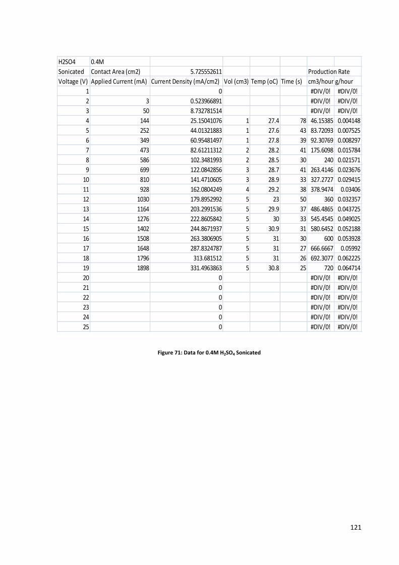
121
H2SO4 0.4M
Sonicated Contact Area (cm2) 5.725552611 Production Rate
Voltage (V) Applied Current (mA) Current Density (mA/cm2) Vol (cm3) Temp (oC) Time (s) cm3/hour g/hour
1 0 #DIV/0! #DIV/0!
2 3 0.523966891 #DIV/0! #DIV/0!
3 50 8.732781514 #DIV/0! #DIV/0!
4 144 25.15041076 1 27.4 78 46.15385 0.004148
5 252 44.01321883 1 27.6 43 83.72093 0.007525
6 349 60.95481497 1 27.8 39 92.30769 0.008297
7 473 82.61211312 2 28.2 41 175.6098 0.015784
8 586 102.3481993 2 28.5 30 240 0.021571
9 699 122.0842856 3 28.7 41 263.4146 0.023676
10 810 141.4710605 3 28.9 33 327.2727 0.029415
11 928 162.0804249 4 29.2 38 378.9474 0.03406
12 1030 179.8952992 5 23 50 360 0.032357
13 1164 203.2991536 5 29.9 37 486.4865 0.043725
14 1276 222.8605842 5 30 33 545.4545 0.049025
15 1402 244.8671937 5 30.9 31 580.6452 0.052188
16 1508 263.3806905 5 31 30 600 0.053928
17 1648 287.8324787 5 31 27 666.6667 0.05992
18 1796 313.681512 5 31 26 692.3077 0.062225
19 1898 331.4963863 5 30.8 25 720 0.064714
20 0 #DIV/0! #DIV/0!
21 0 #DIV/0! #DIV/0!
22 0 #DIV/0! #DIV/0!
23 0 #DIV/0! #DIV/0!
24 0 #DIV/0! #DIV/0!
25 0 #DIV/0! #DIV/0!
Figure 71: Data for 0.4M H2SO4 Sonicated

122
H2SO4 0.5M
Sonicated Contact Area (cm2) 5.725552611 Production Rate
Voltage (V) Applied Current (mA) Current Density (mA/cm2) Vol (cm3) Temp (oC) Time (s) cm3/hour g/hour
1 0 0 #DIV/0! #DIV/0!
2 1 0.17465563 #DIV/0! #DIV/0!
3 59 10.30468219 #DIV/0! #DIV/0!
4 182 31.78732471 1 28.2 92 39.13043 0.003517
5 320 55.88980169 1 28.3 35 102.8571 0.009245
6 464 81.04021245 2 28.7 42 171.4286 0.015408
7 611 106.7145901 3 29.1 43 251.1628 0.022575
8 756 132.0396565 4 29.4 47 306.383 0.027538
9 912 159.2859348 5 29.7 48 375 0.033705
10 1063 185.658935 5 30.1 40 450 0.040446
11 1212 211.6826239 5 29.9 35 514.2857 0.046224
12 1356 236.8330347 5 30.6 32 562.5 0.050558
13 1453 253.7746308 5 31 28 642.8571 0.05778
14 1682 293.7707701 5 31.8 26 692.3077 0.062225
15 1736 303.2021742 5 32.1 23 782.6087 0.070341
16 1950 340.578479 5 32 21 857.1429 0.07704
17 0 #DIV/0! #DIV/0!
18 0 #DIV/0! #DIV/0!
19 0 #DIV/0! #DIV/0!
20 0 #DIV/0! #DIV/0!
21 0 #DIV/0! #DIV/0!
22 0 #DIV/0! #DIV/0!
23 0 #DIV/0! #DIV/0!
24 0 #DIV/0! #DIV/0!
25 0 #DIV/0! #DIV/0!
Figure 72: Data for 0.5M H2SO4 Sonicated

123
H2SO4 1.0M
Sonicated Contact Area (cm2) 4.783074815 Production Rate
Voltage (V) Applied Current (mA) Current Density (mA/cm2) Vol (cm3) Temp (oC) Time (s) cm3/hour g/hour
1 0 0 #DIV/0! #DIV/0!
2 2 0.418141066 #DIV/0! #DIV/0!
3 74 15.47121943 #DIV/0! #DIV/0!
4 279 58.33067865 1 29.2 33 109.0909 0.009805
5 515 107.6713244 2 29.3 38 189.4737 0.01703
6 768 160.5661692 3 29.8 43 251.1628 0.022575
7 1023 213.8791551 5 30.4 43 418.6047 0.037624
8 1305 272.8370453 5 30.9 30 600 0.053928
9 1570 328.2407365 5 31.2 26 692.3077 0.062225
10 1817 379.8811581 5 31.3 21 857.1429 0.07704
11 0 #DIV/0! #DIV/0!
12 0 #DIV/0! #DIV/0!
13 0 #DIV/0! #DIV/0!
14 0 #DIV/0! #DIV/0!
15 0 #DIV/0! #DIV/0!
16 0 #DIV/0! #DIV/0!
17 0 #DIV/0! #DIV/0!
18 0 #DIV/0! #DIV/0!
19 0 #DIV/0! #DIV/0!
20 0 #DIV/0! #DIV/0!
21 0 #DIV/0! #DIV/0!
22 0 #DIV/0! #DIV/0!
23 0 #DIV/0! #DIV/0!
24 0 #DIV/0! #DIV/0!
25 0 #DIV/0! #DIV/0!
Figure 73: Data for 1.0M H2SO4 Sonicated

124
H2SO4
Sonicated 0.1M 0.2M 0.3M 0.4M 0.5M 1.0M
Voltage (V) V ideal Efficiency (%) V ideal Efficiency (%) V ideal Efficiency (%) V ideal Efficiency (%) V ideal Efficiency (%) V ideal Efficiency (%)
1 0 #DIV/0! 0 #DIV/0! 0 #DIV/0! 0 #DIV/0! 0 #DIV/0! 0 #DIV/0!
2 0 #DIV/0! 0 #DIV/0! 0 #DIV/0! 0 #DIV/0! 0 #DIV/0! 0 #DIV/0!
3 0 #DIV/0! 0 #DIV/0! 0 #DIV/0! 0 #DIV/0! 0 #DIV/0! 0 #DIV/0!
4 0 #DIV/0! 0 #DIV/0! 4.635813 21.57118933 2.540242 39.36632707 3.796922 26.33712181 2.507492 39.88047953
5 0 #DIV/0! 2.660383 37.58857184 3.815267 26.21048535 2.452313 40.77782814 2.54059 39.36093557 5.33158 37.51233248
6 3.807301 26.26532315 2.220246 45.04005084 2.603855 38.40459713 3.082376 32.44250213 4.426492 45.18250112 9.011812 33.28964088
7 3.372711 29.64974036 2.655391 37.65923206 2.763607 36.18459154 4.397618 45.47916955 5.975541 50.20465683 12.02779 41.57039639
8 3.266035 30.61816319 2.642672 37.84048716 4.569887 43.76476289 3.990465 50.11947565 8.089433 49.44722276 10.72231 46.63175043
9 3.472197 28.80020975 4.03228 49.59973316 6.556864 45.75357881 6.509588 46.08586736 9.976195 50.11930893 11.19071 44.67989931
10 3.115109 32.10160543 3.252399 61.49306592 5.842781 51.34540967 6.075459 49.37898736 9.702761 51.53172286 10.4641 47.78243654
11 3.021751 33.09339457 3.41272 58.60428822 8.803537 45.43628207 8.023111 49.85596985 9.673558 51.68729154 0 #DIV/0!
12 5.234664 38.20684877 4.987351 60.15217128 8.07561 49.53186348 11.47678 43.56620812 9.918071 50.41302681 0 #DIV/0!
13 5.017978 39.85668997 5.705436 52.58143721 10.81082 46.2499766 9.821329 50.9096059 9.311352 53.69789501 0 #DIV/0!
14 4.863041 41.12653198 5.998613 50.01156112 11.47466 43.57426145 9.605577 52.05309307 10.03527 49.82424778 0 #DIV/0!
15 5.196996 38.48376738 8.951924 44.68313194 10.89258 45.9028282 9.943883 50.28217007 9.171376 54.51744553 0 #DIV/0!
16 5.166409 38.71160517 7.5856 52.73148985 11.4592 43.63305928 10.35408 48.29012291 9.403046 53.17425911 0 #DIV/0!
17 7.650014 39.21561681 9.275104 53.90775108 12.18424 41.03661962 10.1838 49.09756294 0 #DIV/0! 0 #DIV/0!
18 7.460969 40.20925283 8.962999 55.78490091 12.5439 39.86001406 10.68732 46.78441752 0 #DIV/0! 0 #DIV/0!
19 7.207981 41.62053069 8.439517 59.24509592 12.62143 39.61517038 10.85275 46.07128901 0 #DIV/0! 0 #DIV/0!
20 9.283817 43.08572732 8.543032 58.52723103 12.20321 40.9728123 0 #DIV/0! 0 #DIV/0! 0 #DIV/0!
21 9.363266 42.72013671 8.183337 61.09977075 9.77865 51.13180204 0 #DIV/0! 0 #DIV/0! 0 #DIV/0!
22 9.527851 41.98218545 9.060037 55.18741373 9.641194 51.86079676 0 #DIV/0! 0 #DIV/0! 0 #DIV/0!
23 9.788297 40.86512859 9.363072 53.40127622 0 #DIV/0! 0 #DIV/0! 0 #DIV/0! 0 #DIV/0!
24 9.387597 42.60941459 9.492662 52.67226277 0 #DIV/0! 0 #DIV/0! 0 #DIV/0! 0 #DIV/0!
25 8.788992 45.51147638 9.37542 53.33094606 0 #DIV/0! 0 #DIV/0! 0 #DIV/0! 0 #DIV/0!
Figure 74: Data of H2SO4 Efficiency of H2 production

125
Comparison
NaOH
0.1M
Voltage Enhancement in Current Enhancement in Output Enhancement in Efficiency
1 0 #DIV/0! #DIV/0!
2 0.449907966 #DIV/0! #DIV/0!
3 2.549478476 #DIV/0! #DIV/0!
4 1.799631865 #DIV/0! #DIV/0!
5 0.899815933 #DIV/0! #DIV/0!
6 0.899815933 #DIV/0! #DIV/0!
7 1.799631865 -0.018555763 -3.915144055
8 1.499693221 -0.854839255 -4.076830687
9 1.499693221 2.615298088 0.286682159
10 1.499693221 -5.606678777 -8.136685723
11 1.049785255 -15.02489185 -14.6865578
12 0.599877288 -5.632333768 -5.246774107
13 0.749846611 -17.24392041 -13.21925083
14 -0.149969322 -15.79640193 -9.784863477
15 -0.149969322 0 0.252164095
16 -0.299938644 2.307692308 1.51453036
17 0.599877288 11.14551084 4.912665078
18 0.449907966 0 -0.438994898
19 0.899815933 0 -0.819905452
20 0.749846611 -51.28205128 -21.62708528
21 -0.149969322 -24.1509434 -9.05328779
22 0 -19.63636364 -7.0447274
23 -0.299938644 -36.28219485 -12.36416636
24 -0.299938644 -11.62227603 -3.516560578
25 -1.649662543 -52.13705404 -14.89011767
Figure 75: Data for 0.1M NaOH Ultrasound Enhancement

126
0.2M
Voltage Enhancement in Current Enhancement in Output Enhancement in Efficiency
1 0 #DIV/0! #DIV/0!
2 0.895383342 #DIV/0! #DIV/0!
3 3.18186143 #DIV/0! #DIV/0!
4 6.027584725 #DIV/0! #DIV/0!
5 8.273430731 13.0952381 1.666039833
6 10.78744848 10.83333333 -2.683556469
7 13.45143555 -5.704225352 -18.01479131
8 16.71529991 -15.15151515 -27.36507513
9 18.72030848 -14.28571429 -25.50773578
10 23.06129241 -10.24667932 -25.2920519
11 26.92060147 6.315789474 -18.48107347
12 30.53907309 18.36734694 -14.67832865
13 32.7849191 38.0952381 -8.886363501
14 38.34412673 28.57142857 -15.56021654
15 37.99025823 24.3902439 -14.15924174
16 40.98151825 35.52631579 -12.33725965
17 43.91367707 45.40540541 -10.20934388
18 46.81406898 15.82417582 -14.97754468
19 47.89192731 30.85714286 -15.21678541
20 54.07834654 46.37681159 -13.58445451
21 55.06976935 54.85714286 -12.70869119
22 59.4609893 29.8136646 -16.91760302
23 58.68897974 61.91646192 -12.14348309
24 60.00324291 -57.34196117 -25.96335876
25 62.46259204 -16.30434783 -22.68886596
Figure 76: Data for 0.2M NaOH Ultrasound Enhancement

127
0.3M
Voltage Enhancement in Current Enhancement in Output Enhancement in Efficiency
1 0 #DIV/0! #DIV/0!
2 0.782558124 #DIV/0! #DIV/0!
3 2.694614947 #DIV/0! #DIV/0!
4 4.642919293 #DIV/0! #DIV/0!
5 6.274705093 #DIV/0! #DIV/0!
6 7.852766885 -20.21390374 -23.26816513
7 9.562225947 -28.84615385 -25.39994946
8 10.61469866 -70.1754386 -43.28231509
9 13.4769584 -76.35054022 -40.94641423
10 16.13014761 -81.52173913 -38.46091375
11 18.18007447 -121.7391304 -48.01240594
12 21.03650872 -67.76470588 -31.01419007
13 24.53180555 -67.66917293 -32.32170515
14 25.36938224 -66.66666667 -28.56452881
15 26.49952821 -76.23529412 -28.49536175
16 29.06921866 -65.2173913 -25.17658718
17 31.48356259 -85.71428571 -28.54180797
18 31.80137569 -102.0242915 -29.68732171
19 35.15944976 -115.7894737 -31.02567703
20 36.49284077 -143.6170213 -33.82448887
21 38.04695331 -160 -34.9687381
22 39.51756708 -154.2857143 -33.37080746
23 41.5377192 -140 -30.87642458
24 45.21231181 -144.8916409 -31.38513218
25 45.72754446 -181.3953488 -33.32348693
Figure 77: Data for 0.3M NaOH Ultrasound Enhancement

128
0.4M
Voltage Enhancement in Current Enhancement in Output Enhancement in Efficiency
1 0 #DIV/0! #DIV/0!
2 0.698622521 #DIV/0! #DIV/0!
3 1.986013492 #DIV/0! #DIV/0!
4 2.569227522 #DIV/0! #DIV/0!
5 2.926561833 -4.090909091 -7.712041729
6 3.308582452 -32.77310924 -23.99623925
7 3.415350735 -21.71945701 -13.227196
8 3.647402032 5.882352941 -0.434024117
9 3.704797698 -53.68421053 -20.63608479
10 4.910723852 -61.76470588 -21.09951453
11 5.042178443 -28.70813397 -10.324468
12 5.923479645 -28.23529412 -9.63105003
13 6.804780846 -2.470830474 -3.727589019
14 6.311671841 -36.58536585 -9.785660804
15 6.767751384 -25.21008403 -7.43162091
16 6.82514705 -53.61702128 -11.19753729
17 5.608729215 -44.06364749 -8.617567427
18 7.387994877 -44.58204334 -8.819712578
19 7.494763159 -34.34022258 -7.012177487
20 8.448271812 -21.42857143 -5.336111394
21 6.284516902 -90 -12.3003129
22 5.164992826 -94.73684211 -11.7993859
23 6.893034398 -126.0869565 -14.79034699
24 3.282661828 -152.3809524 -15.86191475
25 -0.509772264 -162.8959276 -15.09512084
Figure 78: Data for 0.4M NaOH Ultrasound Enhancement

129
0.5M
Voltage Enhancement in Current Enhancement in Output Enhancement in Efficiency
1 0 #DIV/0! #DIV/0!
2 1.047933782 #DIV/0! #DIV/0!
3 -7.689784994 #DIV/0! #DIV/0!
4 2.742648837 -14.09601634 -13.09105195
5 -7.684847732 -24.61538462 -6.53204861
6 -8.906819987 -44.85049834 -11.44263743
7 -7.907641663 -51.42857143 -11.4680101
8 -9.380179946 -84.7826087 -17.25703172
9 -10.17878201 -61.68910649 -9.093568136
10 -10.22753747 -56.51491366 -6.965114762
11 -9.55113263 -116.3666121 -17.20056495
12 -7.4299616 -84.9213691 -10.9221323
13 -8.503816006 17.54385965 4.847823813
14 -6.056168551 7.653061224 2.428539414
15 -7.803959169 58.60465116 8.85544196
16 -1.255915928 17.14285714 1.948242016
17 -8.681557425 -156.3706564 -14.29249307
18 -9.706039213 -70.58823529 -4.968147546
19 -10.12694077 -97.4025974 -6.891969096
20 -13.46391247 23.80952381 5.102976896
21 -7.426258654 -80 -5.012616794
22 -6.478304421 -54.60060667 -2.962052927
23 -292.4401781 #DIV/0! #DIV/0!
24 -304.1377852 #DIV/0! #DIV/0!
25 0 #DIV/0! #DIV/0!
Figure 79: Data for 0.5M NaOH Ultrasound Enhancement

130
1.0M
Voltage Enhancement in Current Enhancement in Output Enhancement in Efficiency
1 0 #DIV/0! #DIV/0!
2 1.047933782 #DIV/0! #DIV/0!
3 6.844278939 #DIV/0! #DIV/0!
4 11.78092341 26.32411067 4.604616694
5 22.33864026 48.20450396 2.64995109
6 27.67211714 60.90225564 -1.198884875
7 31.72992904 14.2999007 -13.69238177
8 37.88545999 60.92843327 -6.84360856
9 40.12265666 58.64661654 -6.591431992
10 46.69970632 77.5862069 -7.10170606
11 50.75751822 100 -4.225106258
12 48.82581461 112.5 -2.071364918
13 54.38331973 54.54545455 -9.652561541
14 47.28045172 -99.31034483 -22.08295039
15 50.83898304 57.69230769 -7.780633928
16 59.78344964 68.18181818 -8.091303027
17 44.67296042 19.93355482 -8.347644088
18 -299.9386442 #DIV/0! #DIV/0!
19 0 #DIV/0! #DIV/0!
20 0 #DIV/0! #DIV/0!
21 0 #DIV/0! #DIV/0!
22 0 #DIV/0! #DIV/0!
23 0 #DIV/0! #DIV/0!
24 0 #DIV/0! #DIV/0!
25 0 #DIV/0! #DIV/0!
Figure 80: Data for 1.0M NaOH Ultrasound Enhancement
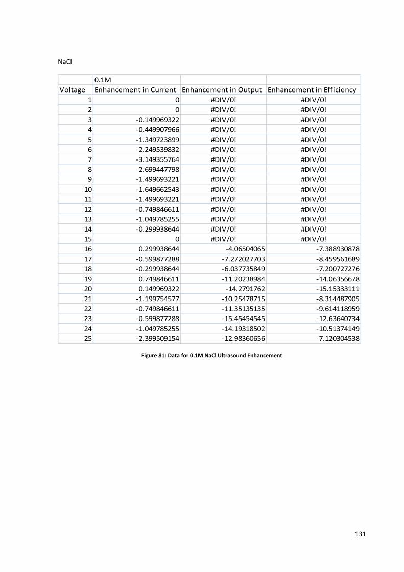
131
NaCl
0.1M
Voltage Enhancement in Current Enhancement in Output Enhancement in Efficiency
1 0 #DIV/0! #DIV/0!
2 0 #DIV/0! #DIV/0!
3 -0.149969322 #DIV/0! #DIV/0!
4 -0.449907966 #DIV/0! #DIV/0!
5 -1.349723899 #DIV/0! #DIV/0!
6 -2.249539832 #DIV/0! #DIV/0!
7 -3.149355764 #DIV/0! #DIV/0!
8 -2.699447798 #DIV/0! #DIV/0!
9 -1.499693221 #DIV/0! #DIV/0!
10 -1.649662543 #DIV/0! #DIV/0!
11 -1.499693221 #DIV/0! #DIV/0!
12 -0.749846611 #DIV/0! #DIV/0!
13 -1.049785255 #DIV/0! #DIV/0!
14 -0.299938644 #DIV/0! #DIV/0!
15 0 #DIV/0! #DIV/0!
16 0.299938644 -4.06504065 -7.388930878
17 -0.599877288 -7.272027703 -8.459561689
18 -0.299938644 -6.037735849 -7.200727276
19 0.749846611 -11.20238984 -14.06356678
20 0.149969322 -14.2791762 -15.15333111
21 -1.199754577 -10.25478715 -8.314487905
22 -0.749846611 -11.35135135 -9.614118959
23 -0.599877288 -15.45454545 -12.63640734
24 -1.049785255 -14.19318502 -10.51374149
25 -2.399509154 -12.98360656 -7.120304538
Figure 81: Data for 0.1M NaCl Ultrasound Enhancement

132
0.2M
Voltage Enhancement in Current Enhancement in Output Enhancement in Efficiency
1 0 #DIV/0! #DIV/0!
2 0.149969322 #DIV/0! #DIV/0!
3 0.299938644 #DIV/0! #DIV/0!
4 0.599877288 #DIV/0! #DIV/0!
5 1.049785255 #DIV/0! #DIV/0!
6 1.499693221 #DIV/0! #DIV/0!
7 1.799631865 #DIV/0! #DIV/0!
8 2.249539832 #DIV/0! #DIV/0!
9 2.699447798 #DIV/0! #DIV/0!
10 3.299325086 1.787576344 -4.713313296
11 3.449294409 -6.98757764 -15.19493415
12 3.449294409 -2.5 -8.655426285
13 2.84941712 -5.555555556 -10.12082264
14 2.399509154 -7.142857143 -10.12736051
15 3.599263731 -4.597701149 -9.320287252
16 2.09957051 -3.126356926 -6.159919556
17 3.299325086 1.902748414 -4.697934543
18 1.199754577 1.993355482 -1.861127192
19 3.149355764 -21.28603104 -15.70050273
20 1.499693221 -34.13793103 -18.93325334
21 2.549478476 0 -4.477100223
22 3.299325086 -7.552447552 -8.789124303
23 0.299938644 -14.1509434 -7.7520159
24 2.84941712 -9.58296362 -8.271550095
25 4.049171697 -13.63636364 -10.92565683
Figure 82: Data for 0.2M NaCl Ultrasound Enhancement

133
0.3M
Voltage Enhancement in Current Enhancement in Output Enhancement in Efficiency
1 0 #DIV/0! #DIV/0!
2 0.059101211 #DIV/0! #DIV/0!
3 1.072686974 #DIV/0! #DIV/0!
4 2.554649832 #DIV/0! #DIV/0!
5 4.332118743 #DIV/0! #DIV/0!
6 6.318658187 #DIV/0! #DIV/0!
7 8.155228309 #DIV/0! #DIV/0!
8 10.01913274 0.491803279 -13.70863716
9 11.70573354 -10.10526316 -25.0959446
10 13.77870851 -6.6359447 -22.31158317
11 15.31090739 -11.84210526 -25.00601266
12 17.86555722 -28.02197802 -33.93078794
13 20.29757204 -16.47597254 -26.76000311
14 22.40231391 -17.2972973 -25.22012049
15 23.54370604 -11.01591187 -19.35622462
16 26.934638 15.2027027 -11.83265295
17 29.63925716 -27.87096774 -29.93935589
18 30.50804496 -18.06020067 -25.34129392
19 34.73082646 -10 -22.99942088
20 33.94034777 3.986710963 -19.01771776
21 36.52233191 0 -20.89723295
22 39.19518416 0 -21.27228415
23 40.06840455 -6.050420168 -22.06560339
24 41.54150223 6.818181818 -19.0005978
25 45.22794024 15 -17.90972194
Figure 83: Data for 0.3M NaCl Ultrasound Enhancement

134
0.4M
Voltage Enhancement in Current Enhancement in Output Enhancement in Efficiency
1 -0.349311261 #DIV/0! #DIV/0!
2 -0.698622521 #DIV/0! #DIV/0!
3 -1.397245042 #DIV/0! #DIV/0!
4 0 #DIV/0! #DIV/0!
5 1.047933782 #DIV/0! #DIV/0!
6 1.746556303 #DIV/0! #DIV/0!
7 2.445178824 -0.767386091 -4.398936023
8 4.366390757 2.395740905 -3.703662033
9 4.017079496 8.975834292 0.806604861
10 6.28760269 6.302521008 -3.485085972
11 6.46225832 -6.818181818 -9.359156907
12 6.636913951 8.586762075 -2.397444782
13 6.986225211 36.26373626 6.795132857
14 10.82864908 7.552447552 -6.8053101
15 11.70192723 21.53846154 -2.730168387
16 9.082092775 40.61538462 4.03977126
17 12.05123849 36.28219485 1.260281106
18 14.14710605 18.9848385 -4.207383094
19 13.97245042 21.0989011 -3.262166935
20 15.71900673 36.51115619 -1.558449956
21 14.14710605 18.90472618 -4.223691604
22 15.89366236 23.41463415 -3.944084547
23 19.91074185 77.64705882 3.599513254
24 23.0545432 32 -6.065109786
25 22.18126505 42.85714286 -3.840074283
Figure 84: Data for 0.4M NaCl Ultrasound Enhancement

135
0.5M
Voltage Enhancement in Current Enhancement in Output Enhancement in Efficiency
1 0 #DIV/0! #DIV/0!
2 0.230670303 #DIV/0! #DIV/0!
3 1.124433662 #DIV/0! #DIV/0!
4 2.184979047 #DIV/0! #DIV/0!
5 3.447276884 #DIV/0! #DIV/0!
6 5.240183668 #DIV/0! #DIV/0!
7 7.413730076 #DIV/0! #DIV/0!
8 6.766777216 -31.16883117 -29.49172035
9 8.461497806 -35.40372671 -28.25205031
10 8.685443027 -38.57634902 -25.83551049
11 12.30084695 -21.4084507 -18.93142315
12 13.64384577 -51.69230769 -30.75478336
13 12.16029275 -37.5 -21.016666
14 15.62572735 -28.980322 -19.42109358
15 16.91089047 -27.15273413 -18.90005079
16 16.42533957 -9.979209979 -12.62702551
17 19.14092756 -23.58722359 -16.29137811
18 21.46982336 -32.14285714 -18.66048313
19 21.45166564 -27.06766917 -17.4323837
20 22.62720992 -7.287449393 -13.04454359
21 25.83305637 -8.571428571 -14.2539865
22 26.85863133 -18.7012987 -15.56132058
23 28.9629094 -17.5 -15.19527621
24 31.32072304 -88.11188811 -26.33024751
25 38.70217273 -8.780487805 -15.34014236
Figure 85: Data for 0.5M NaCl Ultrasound Enhancement
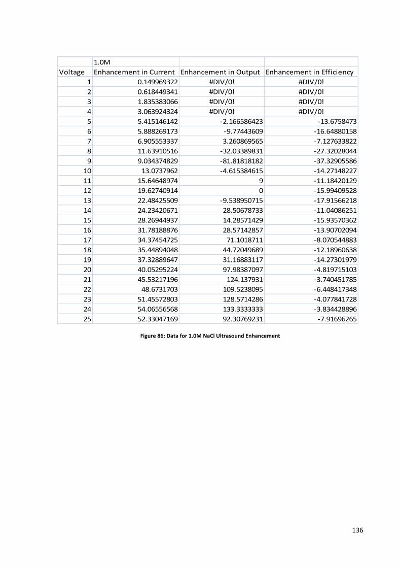
136
1.0M
Voltage Enhancement in Current Enhancement in Output Enhancement in Efficiency
1 0.149969322 #DIV/0! #DIV/0!
2 0.618449341 #DIV/0! #DIV/0!
3 1.835383066 #DIV/0! #DIV/0!
4 3.063924324 #DIV/0! #DIV/0!
5 5.415146142 -2.166586423 -13.6758473
6 5.888269173 -9.77443609 -16.64880158
7 6.905553337 3.260869565 -7.127633822
8 11.63910516 -32.03389831 -27.32028044
9 9.034374829 -81.81818182 -37.32905586
10 13.0737962 -4.615384615 -14.27148227
11 15.64648974 9 -11.18420129
12 19.62740914 0 -15.99409528
13 22.48425509 -9.538950715 -17.91566218
14 24.23420671 28.50678733 -11.04086251
15 28.26944937 14.28571429 -15.93570362
16 31.78188876 28.57142857 -13.90702094
17 34.37454725 71.1018711 -8.070544883
18 35.44894048 44.72049689 -12.18960638
19 37.32889647 31.16883117 -14.27301979
20 40.05295224 97.98387097 -4.819715103
21 45.53217196 124.137931 -3.740451785
22 48.6731703 109.5238095 -6.448417348
23 51.45572803 128.5714286 -4.077841728
24 54.06556568 133.3333333 -3.834428896
25 52.33047169 92.30769231 -7.91696265
Figure 86: Data for 1.0M NaCl Ultrasound Enhancement

137
H2SO4
0.1M
Voltage Enhancement in Current Enhancement in Output Enhancement in Efficiency
1 0 #DIV/0! #DIV/0!
2 0.268171743 #DIV/0! #DIV/0!
3 2.409113101 #DIV/0! #DIV/0!
4 5.58654194 #DIV/0! #DIV/0!
5 8.582234557 #DIV/0! #DIV/0!
6 11.87786582 15.56776557 1.318932683
7 14.69182221 19.93499458 -0.435764272
8 18.25562522 22.42524917 -2.953863864
9 21.57859079 7.714285714 -14.28501746
10 26.09687834 18.14109742 -12.16754696
11 28.01545139 23.37662338 -10.14407725
12 31.33841697 43.87917329 -5.47159676
13 35.02042239 47.50733138 -7.240138305
14 37.2662684 34.61538462 -13.77951397
15 41.21644557 32.95194508 -14.09122904
16 44.48030993 42.07792208 -12.18169945
17 46.12184605 35.52631579 -14.02936766
18 49.65831475 39.74025974 -14.57972266
19 52.8630779 45 -14.82944625
20 56.74972126 51.72413793 -15.01722238
21 62.39979701 43.07692308 -18.1925799
22 64.26370144 57.27272727 -14.9514102
23 66.59598296 26.31229236 -20.31589404
24 71.05073672 41.95804196 -18.86434021
25 72.91020856 134.5054945 -4.214753914
Figure 87: Data for 0.1M H2SO4 Ultrasound Enhancement

138
0.2M
Voltage Enhancement in Current Enhancement in Output Enhancement in Efficiency
1 0 #DIV/0! #DIV/0!
2 -0.024686308 #DIV/0! #DIV/0!
3 0.882535517 #DIV/0! #DIV/0!
4 0.648632747 #DIV/0! #DIV/0!
5 -0.631352331 8.067226891 7.782314671
6 -1.936023718 1.411764706 3.037229842
7 -3.789348304 3.260869565 4.228804987
8 -4.993422984 -7.05052879 0.440568742
9 -5.922245329 12.01501877 7.392020354
10 -8.225477881 38.18181818 15.43026452
11 -8.030456047 15 7.905570688
12 -14.9561998 23.41463415 12.54897415
13 -10.7860652 6.585365854 5.513069425
14 -11.61429083 -15.78947368 1.36940532
15 -12.19380192 -31.64835165 -1.331637345
16 -15.07037398 23.94678492 7.958596441
17 -15.87206184 5.590062112 5.215500367
18 -20.94694964 17.14285714 7.708459409
19 -19.50465208 62.95707472 12.30523448
20 -21.70358498 64.28571429 12.1351329
21 -23.18476347 97.98387097 15.51164736
22 -23.36003626 -30.54545455 2.060956249
23 -22.13806401 -37.5 0.905245119
24 -23.71798773 -45.44179523 0.286848031
25 -22.74843298 -71.61803714 -2.170593081
Figure 88: Data for 0.2M H2SO4 Ultrasound Enhancement

139
0.3M
Voltage Enhancement in Current Enhancement in Output Enhancement in Efficiency
1 0 #DIV/0! #DIV/0!
2 0.049372616 #DIV/0! #DIV/0!
3 1.460195128 #DIV/0! #DIV/0!
4 6.778243065 -19.28571429 -29.4129962
5 3.857235651 -17.00404858 -13.50824021
6 3.952895095 -22.7027027 -12.42830001
7 5.272995424 -47.44186047 -18.14105223
8 4.392928538 -45 -13.59244582
9 4.712616229 -45 -11.6036299
10 5.83337462 -42.99182904 -10.42018014
11 7.199144619 -60 -12.11361603
12 12.43387627 -44.58204334 -10.56877856
13 12.92821959 -108.6956522 -17.59426288
14 15.56780309 -120.3208556 -17.7703468
15 10.81877455 -138.4615385 -17.170391
16 7.06460424 -161.6099071 -16.9898477
17 13.17631698 -205.8212058 -20.92631625
18 7.05102677 -250 -21.81440392
19 9.494971279 -288.7700535 -24.03612886
20 20.29584826 -257.1428571 -22.10040691
21 325.7327505 #DIV/0! #DIV/0!
22 335.862777 #DIV/0! #DIV/0!
23 0 #DIV/0! #DIV/0!
24 0 #DIV/0! #DIV/0!
25 0 #DIV/0! #DIV/0!
Figure 89: Data for 0.3M H2SO4 Ultrasound Enhancement

140
0.4M
Voltage Enhancement in Current Enhancement in Output Enhancement in Efficiency
1 0 #DIV/0! #DIV/0!
2 0.224028247 #DIV/0! #DIV/0!
3 0.934376764 #DIV/0! #DIV/0!
4 0.705411256 2.780352178 1.379736035
5 0.522115418 -7.418310274 -4.086474797
6 -2.78214693 -64.21404682 -20.1324943
7 -1.820615227 -54.17747794 -12.78626903
8 -3.230203424 -51.89189189 -9.069781498
9 -5.089699586 -105.8161351 -16.07192051
10 -7.598445654 -72.72727273 -8.067982244
11 -10.08435689 -166.507177 -17.97221488
12 -15.06481956 -240 -22.32104702
13 -12.95660884 -180.1801802 -15.08933976
14 -17.69020843 -174.5454545 -12.02678101
15 -15.9294575 -201.9635344 -13.96272206
16 -30.40921156 -218.1818182 -11.3322018
17 287.8324787 #DIV/0! #DIV/0!
18 313.681512 #DIV/0! #DIV/0!
19 331.4963863 #DIV/0! #DIV/0!
20 0 #DIV/0! #DIV/0!
21 0 #DIV/0! #DIV/0!
22 0 #DIV/0! #DIV/0!
23 0 #DIV/0! #DIV/0!
24 0 #DIV/0! #DIV/0!
25 0 #DIV/0! #DIV/0!
Figure 90: Data for 0.4M H2SO4 Ultrasound Enhancement

141
0.5M
Voltage Enhancement in Current Enhancement in Output Enhancement in Efficiency
1 0 #DIV/0! #DIV/0!
2 -0.17465563 #DIV/0! #DIV/0!
3 1.222589412 #DIV/0! #DIV/0!
4 2.095867563 -1.778656126 -3.160313847
5 1.921211933 -21.28078818 -9.883751119
6 0.349311261 2.678571429 0.409607712
7 -3.143801345 21.37555666 5.424190972
8 -6.46225832 -13.61702128 -0.016881199
9 -8.034158993 -34.09090909 -2.224783567
10 -14.84572857 -36.48648649 -0.413097444
11 -31.43801345 -31.16883117 3.655068723
12 -17.46556303 -37.5 -0.099981135
13 -30.91404656 -49.45054945 1.635408288
14 -19.91074185 -57.69230769 -1.36376695
15 -40.86941749 0 5.821612669
16 340.578479 #DIV/0! #DIV/0!
17 0 #DIV/0! #DIV/0!
18 0 #DIV/0! #DIV/0!
19 0 #DIV/0! #DIV/0!
20 0 #DIV/0! #DIV/0!
21 0 #DIV/0! #DIV/0!
22 0 #DIV/0! #DIV/0!
23 0 #DIV/0! #DIV/0!
24 0 #DIV/0! #DIV/0!
25 0 #DIV/0! #DIV/0!
Figure 91: Data for 0.5M H2SO4 Ultrasound Enhancement

142
1.0M
Voltage Enhancement in Current Enhancement in Output Enhancement in Efficiency
1 0 #DIV/0! #DIV/0!
2 -0.804448346 #DIV/0! #DIV/0!
3 0.450835223 #DIV/0! #DIV/0!
4 8.728479651 3.20855615 -5.518270322
5 11.43607211 -30.93447905 -11.19728587
6 10.01301589 -121.2510024 -19.31900724
7 11.45327956 -110.8071135 -14.05188557
8 14.87067938 -42.85714286 -6.36785405
9 15.78181392 -90.30100334 -8.588908698
10 379.8811581 #DIV/0! #DIV/0!
11 0 #DIV/0! #DIV/0!
12 0 #DIV/0! #DIV/0!
13 0 #DIV/0! #DIV/0!
14 0 #DIV/0! #DIV/0!
15 0 #DIV/0! #DIV/0!
16 0 #DIV/0! #DIV/0!
17 0 #DIV/0! #DIV/0!
18 0 #DIV/0! #DIV/0!
19 0 #DIV/0! #DIV/0!
20 0 #DIV/0! #DIV/0!
21 0 #DIV/0! #DIV/0!
22 0 #DIV/0! #DIV/0!
23 0 #DIV/0! #DIV/0!
24 0 #DIV/0! #DIV/0!
25 0 #DIV/0! #DIV/0!
Figure 92: Data for 1.0M H2SO4 Ultrasound Enhancement

143
7.2 Appendix II - Graphs
7.2.1 Preliminary Experiments
Silent
Figure 93: Current Voltage Graph for Silent NaOH solution
Figure 94: Current Voltage Graph for Silent NaCl solution
0
200
400
600
800
1000
1200
1400
1600
1800
2000
0 5 10 15 20 25
Cu
rre
nt
/ m
A
Voltage / V
NaOH
0.1M Unsonicated
0.2M Unsonicated
0.3M Unsonicated
0.4M Unsonicated
0.5M Unsonicated
1.0M Unsonicated
0
200
400
600
800
1000
1200
1400
1600
1800
2000
0 5 10 15 20 25
Cu
rre
nt
/ m
A
Voltage / V
NaCl
0.1M Unsonicated
0.2M Unsonicated
0.3M Unsonicated
0.4M Unsonicated
0.5M Unsonicated
1.0M Unsonicated

144
Figure 95: Current Voltage Graph for Silent H2SO4 solution
Sonicated
Figure 96: Current Voltage Graph for Sonicated NaOH solution
0
200
400
600
800
1000
1200
1400
1600
1800
2000
0 5 10 15 20 25
Cu
rre
nt
/ m
A
Voltage / V
H2SO4
0.1M Unsonicated
0.2M Unsonicated
0.3M Unsonicated
0.4M Unsonicated
0.5M Unsonicated
1.0M Unsonicated
0
200
400
600
800
1000
1200
1400
1600
1800
2000
0 5 10 15 20 25
Cu
rre
nt
/ m
A
Voltage / V
NaOH
0.1M Sonicated
0.2M Sonicated
0.3M Sonicated
0.4M Sonicated
0.5M Sonicated
1.0M Sonicated

145
Figure 97: Current Voltage Graph for Sonicated NaCl solution
Figure 98: Current Voltage Graph for Sonicated H2SO4 solution
0
200
400
600
800
1000
1200
1400
1600
1800
2000
0 5 10 15 20 25
Cu
rre
nt
/ m
A
Voltage / V
NaCl
0.1M Sonicated
0.2M Sonicated
0.3M Sonicated
0.4M Sonicated
0.5M Sonicated
1.0M Sonicated
0
200
400
600
800
1000
1200
1400
1600
1800
2000
0 5 10 15 20 25
Cu
rre
nt
/ m
A
Voltage / V
H2SO4
0.1M Sonicated
0.2M Sonicated
0.3M Sonicated
0.4M Sonicated
0.5M Sonicated
1.0M Sonicated

146
7.2.2 Custom Glassware Experiments
Silent
Figure 99: Current Voltage Graph for Silent NaOH solution
Figure 100: Current Voltage Graph for Silent NaCl solution
0
50
100
150
200
250
300
0 5 10 15 20 25
Cu
rre
nt
De
nsi
ty /
mA
.cm
-2
Voltage / V
NaOH Unsonicated
0.1M
0.2M
0.3M
0.4M
0.5M
1.0M
0
50
100
150
200
0 5 10 15 20 25
Cu
rre
nt
De
nsi
ty /
mA
.cm
-2
Voltage / V
NaCl Unsonicated
0.1M
0.2M
0.3M
0.4M
0.5M
1.0M

147
Figure 101: Current Voltage Graph for Silent H2SO4 solution
Sonicated
Figure 102: Current Voltage Graph for Sonicated NaOH solution
0
50
100
150
200
250
300
350
0 5 10 15 20 25
Cu
rre
nt
De
nsi
ty /
mA
.cm
-2
Voltage / V
H2SO4 Unsonicated
0.1M
0.2M
0.3M
0.4M
0.5M
1.0M
0
50
100
150
200
250
300
350
0 5 10 15 20 25
Cu
rre
nt
De
nsi
ty /
mA
.cm
-2
Voltage/ V
NaOH Sonicated
0.1M
0.2M
0.3M
0.4M
0.5M
1.0M

148
Figure 103: Current Voltage Graph for Sonicated NaCl solution
Figure 104: Current Voltage Graph for Sonicated H2SO4 solution
0
50
100
150
200
250
0 5 10 15 20 25
Cu
rre
nt
De
nsi
ty /
mA
.cm
-2
Voltage / V
NaCl Sonicated
0.1M
0.2M
0.3M
0.4M
0.5M
1.0M
0
50
100
150
200
250
300
350
400
0 5 10 15 20 25
Cu
rre
nt
De
nsi
ty /
mA
.cm
-2
Voltage / V
H2SO4 Sonicated
0.1M
0.2M
0.3M
0.4M
0.5M
1.0M

149
Figure 105: Hydrogen Production Graph for Silent NaOH solution
Figure 106: Hydrogen Production Graph for Silent NaCl solution
0
100
200
300
400
500
600
700
800
900
0 5 10 15 20 25
Pro
du
ctio
n R
ate
/ c
m3.h
r-1
Voltage / V
NaOH Unsonicated
0.1M
0.2M
0.3M
0.4M
0.5M
1.0M
0
100
200
300
400
500
600
0 5 10 15 20 25
Pro
du
ctio
n R
ate
/ c
m3.h
r-1
Voltage / V
NaCl Unsonicated
0.1M
0.2M
0.3M
0.4M
0.5M
1.0M

150
Figure 107: Hydrogen Production Graph for Silent H2SO4 solution
Figure 108: Hydrogen Production Graph for Sonicated NaOH solution
0
100
200
300
400
500
600
700
800
900
0 5 10 15 20 25
Pro
du
ctio
n R
ate
/ c
m3.h
r-1
Voltage / V
H2SO4 Unsonicated
0.1M
0.2M
0.3M
0.4M
0.5M
1.0M
0
100
200
300
400
500
600
700
800
900
0 5 10 15 20 25
Pro
du
ctio
n R
ate
/ c
m3 .
hr-1
Voltage / V
NaOH Sonicated
0.1M
0.2M
0.3M
0.4M
0.5M
1.0M

151
Figure 109: Hydrogen Production Graph for Sonicated NaCl solution
Figure 110: Hydrogen Production Graph for Sonicated H2SO4 solution
0
100
200
300
400
500
600
700
0 5 10 15 20 25
Pro
du
ctio
n R
ate
/ c
m3.h
r-1
Voltage / V
NaCl Sonicated
0.1M
0.2M
0.3M
0.4M
0.5M
1.0M
0
100
200
300
400
500
600
700
800
900
0 5 10 15 20 25
Pro
du
ctio
n R
ate
/ c
m3 .
hr-1
Voltage / V
H2SO4 Sonicated
0.1M
0.2M
0.3M
0.4M
0.5M
1.0M
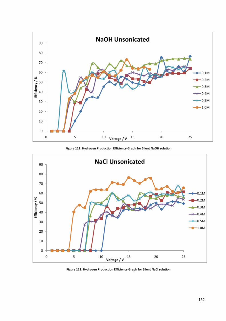
152
Figure 111: Hydrogen Production Efficiency Graph for Silent NaOH solution
Figure 112: Hydrogen Production Efficiency Graph for Silent NaCl solution
0
10
20
30
40
50
60
70
80
90
0 5 10 15 20 25
Effi
cie
ncy
/ %
Voltage / V
NaOH Unsonicated
0.1M
0.2M
0.3M
0.4M
0.5M
1.0M
0
10
20
30
40
50
60
70
80
90
0 5 10 15 20 25
Effi
cie
ncy
/ %
Voltage / V
NaCl Unsonicated
0.1M
0.2M
0.3M
0.4M
0.5M
1.0M

153
Figure 113: Hydrogen Production Efficiency Graph for Silent H2SO4 solution
Sonicated
Figure 114: Hydrogen Production Efficiency Graph for Sonicated NaOH solution
0
10
20
30
40
50
60
70
80
0 5 10 15 20 25
Effi
cie
ncy
/ %
Voltage / V
H2SO4 Unsonicated
0.1M
0.2M
0.3M
0.4M
0.5M
1.0M
0
10
20
30
40
50
60
70
0 5 10 15 20 25
Effi
cie
ncy
/ %
Voltage / V
NaOH Sonicated
0.1M
0.2M
0.3M
0.4M
0.5M
1.0M

154
Figure 115: Hydrogen Production Efficiency Graph for Sonicated NaCl solution
Figure 116: Hydrogen Production Efficiency Graph for Sonicated H2SO4 solution
0
10
20
30
40
50
60
70
0 5 10 15 20 25 30
Effi
cie
ncy
/ %
Voltage / V
NaCl Sonicated
0.1M
0.2M
0.3M
0.4M
0.5M
1.0M
0
10
20
30
40
50
60
70
0 5 10 15 20 25
Effi
cie
ncy
/ %
Voltage/ V
H2SO4 Sonicated
0.1M
0.2M
0.3M
0.4M
0.5M
1.0M

155
7.3 Appendix III – Decomposition Potential Calculations
Graphs
0
200
400
600
800
1000
1200
1400
1600
1800
2000
0 5 10 15 20 25
Cu
rre
nt
/ m
A
Voltage / V
NaOH
0.1M Unsonicated0.1M Sonicated0.2M Unsonicated0.2M Sonicated0.3M Unsonicated0.3M Sonicated0.4M Unsonicated0.4M Sonicated0.5M Unsonicated0.5M Sonicated1.0M Unsonicated1.0M Sonicated
0
200
400
600
800
1000
1200
1400
1600
1800
2000
0 5 10 15 20 25
Cu
rre
nt
/ m
A
Voltage / V
NaCl
0.1M Unsonicated0.2M Unsonicated0.2M Sonicated0.3M Unsonicated0.3M Sonicated0.4M Unsonicated0.4M Sonicated0.5M Unsonicated0.5M Sonicated1.0M Unsonicated1.0M Sonicated
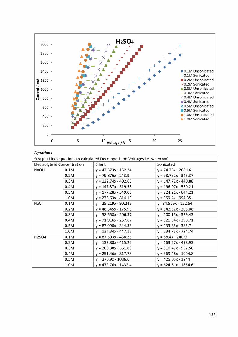
156
Equations
Straight Line equations to calculated Decomposition Voltages i.e. when y=0
Electrolyte & Concentration Silent Sonicated
NaOH 0.1M y = 47.573x - 152.24 y = 74.76x - 268.16
0.2M y = 79.876x - 243.9 y = 98.762x - 345.37
0.3M y = 122.74x - 402.65 y = 147.72x - 440.88
0.4M y = 147.37x - 519.53 y = 196.07x - 550.21
0.5M y = 177.28x - 549.03 y = 224.21x - 644.21
1.0M y = 278.63x - 814.13 y = 359.4x - 994.35
NaCl 0.1M y = 25.219x - 90.245 y =34.525x - 122.54
0.2M y = 48.345x - 175.93 y = 54.532x - 205.08
0.3M y = 58.558x - 206.37 y = 100.15x - 329.43
0.4M y = 71.916x - 257.67 y = 121.54x - 398.71
0.5M y = 87.998x - 344.38 y = 133.85x - 385.7
1.0M y = 134.34x - 447.12 y = 234.73x - 724.74
H2SO4 0.1M y = 87.593x - 438.25 y = 88.4x - 240.9
0.2M y = 132.88x - 415.22 y = 163.57x - 498.93
0.3M y = 200.38x - 561.83 y = 310.47x - 952.58
0.4M y = 251.46x - 817.78 y = 369.48x - 1094.8
0.5M y = 370.9x - 1086.6 y = 425.05x - 1244
1.0M y = 472.76x - 1432.4 y = 624.61x - 1854.6
0
200
400
600
800
1000
1200
1400
1600
1800
2000
0 5 10 15 20 25
Cu
rre
nt
/ m
A
Voltage / V
H2SO4
0.1M Unsonicated0.1M Sonicated0.2M Unsonicated0.2M Sonicated0.3M Unsonicated0.3M Sonicated0.4M Unsonicated0.4M Sonicated0.5M Unsonicated0.5M Sonicated1.0M Unsonicated1.0M Sonicated

157
Industrial Electrolyser Decomposition Voltages
Straight Line equations to calculated Decomposition Voltages i.e. when y=0
Electrolyte & Concentration Equation
KOH 0.1M y = 43.5x – 122.5
0.3M y = 86.7x – 130.3
0.5M y = 169.8x – 465.2
0
100
200
300
400
500
600
700
800
900
1000
0 2 4 6 8 10
Cu
rre
nt
/ m
A
Voltage / V
0.1M KOH
0.3M KOH
0.5M KOH

158
7.4 Appendix IV - Ultrasound Power Data Tables
Temperature (K) Amplitude
Time (seconds) 20 25 30 35 40
Water
0 297.8 297.9 297.8 297.9 298
5 298.1 298.2 298.5 298.5 298.8
10 298.1 298.3 298.3 298.3 298.5
15 298 298.4 298.3 298.3 298.4
20 298.2 298.6 298.4 298.4 298.4
25 298.3 298.5 298.6 298.6 298.5
30 298.2 298.6 298.5 298.5 298.6
NaOH
0 294.1 294.4 294.4 294.5 294.6
5 294.2 294.5 294.6 294.7 294.8
10 294.3 294.5 294.7 294.7 294.9
15 294.3 294.5 294.7 294.7 294.9
20 294.3 294.6 294.8 294.7 294.9
25 294.3 294.4 294.8 294.8 294.9
30 294.4 294.5 294.8 294.8 295.2
NaCl
0 294.2 294.5 294.9 295.2 295.3
5 294.3 294.6 295 295.3 295.4
10 294.4 294.8 295.1 295.4 295.4
15 294.4 294.6 295.1 295.4 295.5
20 294.4 294.7 295.1 295.5 295.4
25 294.4 294.7 295.1 295.5 295.5
30 294.4 294.7 295.1 295.5 295.5
H2SO4
0 291.5 291.6 291.8 292 292.1
5 291.8 291.8 292 292.3 292.5
10 292 291.9 292.2 292.4 292.6
15 291.9 291.9 292.3 292.5 292.7
20 291.8 292 292.3 292.5 292.6
25 291.9 292.1 292.3 292.6 292.7
30 291.8 292.1 292.4 292.5 292.7
Figure 117: Temperature variance table for each electrolyte at varying ultrasonic powers
Temperature Gradient (dT/dt)
20 25 30 35 40
Water 0.08 0.12 0.2 0.16 0.24
NaOH 0.023 0.08 0.06 0.066 0.04
NaCl 0.02 0.048 0.02 0.032 0.03
H2SO4 0.066 0.08 0.06 0.1 0.14
Figure 118: dT/dt gradients calculated for each electrolyte
Ultrasound Power (W)
Amplitude 20 25 30 35 40
Water 334.4 501.6 836.0 668.8 1003.2
NaOH 76.8 267.0 200.3 220.3 133.5
NaCl 79.9 191.6 79.9 127.8 119.8
H2SO4 94.1 114.1 85.6 142.6 199.7
Figure 119: Ultrasound Power Table

159
7.5 Appendix V - Health & Safety
Appendix Vi - COSHH Forms

160

161

162
Appendix Vii - Risk Assessment Form

163
7.6 Appendix VI – Conferences Attended & Posters Presented
Poster Presented on next page was presented at the following Conferences.
6th International Conference in HFC, NEC, Birmingham, 25th March 25th March 2010
MEG Annual Meeting, Leicester University, April 2010
Sustainability Conference, NEC, Birmingham, May 2010

164