Embed Size (px)
Citation preview
Sonia Fiol Gonzalez
A novel committee - based clustering method
Dissertacao de Mestrado
Dissertation presented to the Programa de Pos-Graduacao emInformatica of the Departamento de Informatica, PUC-Rio aspartial fulfillment of the requirements for the degree of Mestreem Informatica
Advisor: Prof. Helio Cortes Vieira Lopes
Rio de JaneiroSeptember 2016
Sonia Fiol Gonzalez
A novel committee - based clustering method
Dissertation presented to the Programa de Pos-Graduacao emInformatica of the Departamento de Informatica, PUC-Rio aspartial fulfillment of the requirements for the degree of Mestreem Informatica. Approved by the following commission:
Prof. Helio Cortes Vieira LopesAdvisor
Departamento de Informatica — PUC-Rio
Prof. Pedro Carvalho Loureiro de SouzaDepartamento de Economia — PUC-Rio
Prof. Marcus Vinicius Soledade Poggi de AragaoDepartamento de Informatica — PUC-Rio
Prof. Simone Diniz Junqueira BarbosaDepartamento de Informatica — PUC-Rio
Prof. Marcio da Silveira CarvalhoCoordinator of the Centro Tecnico Cientıfico — PUC-Rio
Rio de Janeiro, September 15, 2016
All rights reserved.
Sonia Fiol Gonzalez
The author graduated in Computer Science from Universityof Havana in 2012, she has interest in Data Science, MachineLearning and Information Visualization.
Bibliographic data
Gonzalez, Sonia
A novel committee - based clustering method / Sonia FiolGonzalez ; advisor: Helio Cortes Vieira Lopes. — 2016.
70 f. : il. ; 30 cm
Dissertacao (Mestrado em Informatica)-Pontifıcia Univer-sidade Catolica do Rio de Janeiro, Rio de Janeiro, 2016.
Inclui bibliografia
1. Informatica – Teses. 2. Selecao de atributos. 3. Metodosde agrupamento. 4. Matriz de similaridade. 5. Aprendizagemnao supervisionada. I. Lopes, Helio. II. Pontifıcia UniversidadeCatolica do Rio de Janeiro. Departamento de Informatica. III.Tıtulo.
CDD: 004

Acknowledgments
In first place, to my advisor, Helio Lopes, for the opportunity, confidence,
creativity, passion and dedication to the research and for the valuable teachings
through this period. To professors Simone Barbosa, for all life and professional
advices, and Marcus Poggi, for providing the means for this research.
To my family, in particular my parents and my sister, for the love,
affection and unconditional support through these two years of sacrifice. To my
best friend Delvia, for her constant concern and advise even being far away.
To Cassio and Rafael, my first Brazilian friends. Cassio, for his honest
friendship, teachings, incentive, company and constant brainstorm. Rafael, for
his friendship, support and for helping me see this wonderful opportunity. Also
to their families for making me feel at home.
To Jefry, for his infinite patience and understanding in this period filled
with tension and for his innumerable advices in order to finish the thesis on
time.
To my colleagues William, Pedro, Jonatas, Luiz and Guilherme, for
providing me a special environment and spirit. Also for their friendship and
will to contribute to this work.
To Liander, Ema, Liester and the big Cuban community, for their help
to reduce the homesickness.
To all those new friends that somehow contributed to my well-being that
turned my stay in Rio more special.
For you all, my sincere thank you!
Abstract
Gonzalez, Sonia; Lopes, Helio (advisor). A novel committee - basedclustering method. Rio de Janeiro, 2016. 70p. Dissertacao de Mestrado— Departamento de Informatica, Pontifıcia Universidade Catolica do Riode Janeiro.
In data analysis, in the process of quantitative modeling and in
the construction of decision support models, clustering, classification and
information retrieval algorithms are very useful. For these algorithms it is
crucial to determine the relevant features in the original dataset. To deal with
this problem, techniques for feature selection play an important role. Moreover,
it is recognized that in unsupervised learning tasks it is also difficult to define
the correct number of clusters. This research proposes a method based on
ensemble methods using all features from a dataset and varying the number
of clusters to calculate the similarity matrix between any two instances of the
dataset. Each element in this matrix stores the probability of the corresponding
instances to be in the same cluster in these multiple scenarios. Notice that the
similarity matrix might be transformed to a distance matrix to be used in other
clustering methods. The experiments were made with a real-world dataset of
the crimes in Rio de Janeiro Capital showing the effectiveness of the proposed
technique.
KeywordsFeature selection; Clustering methods; Similarity matrix; Unsuper-
vised learning;
Resumo
Gonzalez, Sonia; Lopes, Helio. Um novo metodo de agrupamentobaseado em comite. Rio de Janeiro, 2016. 70p. Dissertacao deMestrado — Departamento de Informatica, Pontifıcia UniversidadeCatolica do Rio de Janeiro.
Na analise de dados, no processo de modelagem quantitativa e na
construcao de modelos para suporte a decisoes, os algoritmos de agrupamento,
classificacao e recuperacao de informacao sao muito uteis. Para estes algoritmos
e crucial determinar quais atributos sao relevantes no dataset. Para lidar
com esses problemas, tecnicas de selecao de atributos possuem um papel
importante. Alem disso, e sabido que na tarefa de aprendizagem nao
supervisionada e difıcil definir o numero ideal de agrupamentos. Este trabalho
propoe um metodo baseado em um conjunto de metodos usando todos os
atributos do dataset e variando o numero de agrupamentos para calcular
uma matriz de similaridade entre as instancias do dataset. Cada elemento
desta matriz representa a probabilidade das instancias associadas estarem
no mesmo agrupamento nos multiplos cenarios. Esta matriz de similaridade
pode ser transformada numa matriz de distancia e aplicada em metodos de
agrupamentos. O experimento foi feito com um dataset real dos dados de crimes
na capital do Rio de Janeiro, que por sua natureza mostra a necessidade do
uso do metodo proposto.
Palavras-chaveSelecao de atributos; Metodos de agrupamento; Matriz de similari-
dade; Aprendizagem nao supervisionada;

Contents
1 Introduction 10
2 Theoretical Background 122.1 Clustering Algorithms 122.2 Feature Selection Algorithms 152.3 Ensemble Clustering 182.4 Discussion 19
3 Method for calculating the similarity matrix 20
4 Visual Exploration Tools based on the Similarity Matrix 254.1 Similarity Matrix as a Heat Map 264.2 Similarity Matrix as a Hierarchical Edge Bundling 274.3 Similarity Matrix as a Graph 284.4 Clustering Solution in Map 294.5 Discussion 29
5 Experiments and Results 305.1 Performances of our Method 305.2 Exploring Real World Datasets 355.3 Discussion 50
6 Conclusion and Future Work 51
Bibliography 53
A Appendix 59
B Appendix 60
C Appendix 69
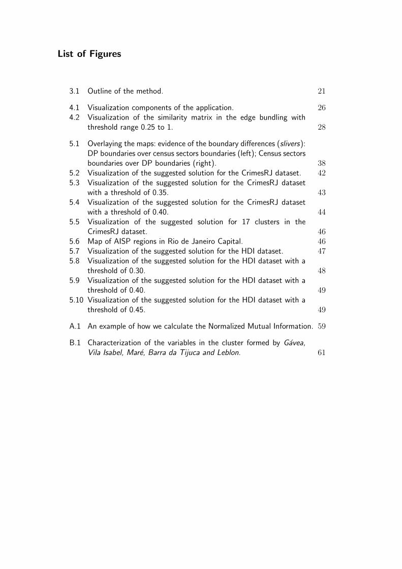
List of Figures
3.1 Outline of the method. 21
4.1 Visualization components of the application. 264.2 Visualization of the similarity matrix in the edge bundling with
threshold range 0.25 to 1. 28
5.1 Overlaying the maps: evidence of the boundary differences (slivers):DP boundaries over census sectors boundaries (left); Census sectorsboundaries over DP boundaries (right). 38
5.2 Visualization of the suggested solution for the CrimesRJ dataset. 425.3 Visualization of the suggested solution for the CrimesRJ dataset
with a threshold of 0.35. 435.4 Visualization of the suggested solution for the CrimesRJ dataset
with a threshold of 0.40. 445.5 Visualization of the suggested solution for 17 clusters in the
CrimesRJ dataset. 465.6 Map of AISP regions in Rio de Janeiro Capital. 465.7 Visualization of the suggested solution for the HDI dataset. 475.8 Visualization of the suggested solution for the HDI dataset with a
threshold of 0.30. 485.9 Visualization of the suggested solution for the HDI dataset with a
threshold of 0.40. 495.10 Visualization of the suggested solution for the HDI dataset with a
threshold of 0.45. 49
A.1 An example of how we calculate the Normalized Mutual Information. 59
B.1 Characterization of the variables in the cluster formed by Gavea,Vila Isabel, Mare, Barra da Tijuca and Leblon. 61
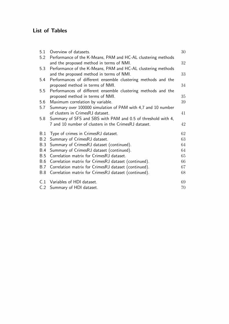
List of Tables
5.1 Overview of datasets. 305.2 Performance of the K-Means, PAM and HC-AL clustering methods
and the proposed method in terms of NMI. 325.3 Performance of the K-Means, PAM and HC-AL clustering methods
and the proposed method in terms of NMI. 335.4 Performances of different ensemble clustering methods and the
proposed method in terms of NMI. 345.5 Performances of different ensemble clustering methods and the
proposed method in terms of NMI. 355.6 Maximum correlation by variable. 395.7 Summary over 100000 simulation of PAM with 4,7 and 10 number
of clusters in CrimesRJ dataset. 415.8 Summary of SFS and SBS with PAM and 0.5 of threshold with 4,
7 and 10 number of clusters in the CrimesRJ dataset. 42
B.1 Type of crimes in CrimesRJ dataset. 62B.2 Summary of CrimesRJ dataset. 63B.3 Summary of CrimesRJ dataset (continued). 64B.4 Summary of CrimesRJ dataset (continued). 64B.5 Correlation matrix for CrimesRJ dataset. 65B.6 Correlation matrix for CrimesRJ dataset (continued). 66B.7 Correlation matrix for CrimesRJ dataset (continued). 67B.8 Correlation matrix for CrimesRJ dataset (continued). 68
C.1 Variables of HDI dataset. 69C.2 Summary of HDI dataset. 70
1Introduction
Nowadays, biomedicine, bioinformatics, sociology, economy, marketing, pat-
tern recognition and computer vision are examples of research areas that use
Machine Learning to generalize behaviours. In this context, machine learning
techniques come to reveal the natural structure of the data in such areas. A
specific kind of problem within machine learning is to group the elements of
a dataset according to their similarities. This is typically called a clustering
problem, which is classified as an unsupervised learning problem. In unsuper-
vised learning there is no known association of a value (discrete/continuous) to
each element in the dataset. In particular, clustering is a challenging problem
due to the lack of generalized algorithms. Instead, there are specific domain
solutions using particular key details according to the application area [58].
On one hand, feature selection has become an important tool for de-
cision support systems that use thousands of features [11]. The importance
of this technique is not only in the reduction of execution time, but also in
the improvement of the clustering quality. There are two different classifica-
tions: attribute selection [9, 27] and attribute transformation [15, 28]. These
techniques are being widely used to remove related or irrelevant attributes
in machine learning algorithms: in supervised learning [8, 13] as well as in
unsupervised learning [21].
On the other hand, another technique that has been accepted by the
scientific community is the use of committees in machine learning [62]. This
is because it has proven to be effective and versatile solving real life problems
combined with machine learning techniques [45, 16].
The objective of this work is to improve clustering results by combining
multiple clustering and feature selection algorithms. To do so, we propose
a committee-based technique using feature selection algorithms and different
clustering methods to generate a matrix where the position i, j contains the
probability of the element i and the element j to be in the same cluster. In
addition, this work explores the resulting matrix not only as a distance matrix
for clustering generation [24], but also as an adjacency matrix with weights
where statistical network analysis [37] can be applied. Finally we developed a
A novel committee - based clustering method 11
web application with visual tools to explore and analyze the results.
In summary, the main contributions of this work are:
– A method to obtain a consensus method in unsupervised learning.
– A web application with visual tools to explore the relations between the
elements of the dataset.
This dissertation is organized as follows. Section 2 presents the theoretical
background. Section 3 explains in details the proposed method. Section 4
describes the visual exploration tool. Section 5 presents the experiments and
the results in seven known datasets and explores two complex real-world
datasets. Finally, Section 6 presents the conclusions and suggests future work.
2Theoretical Background
This chapter presents a literature review with some of the most relevant
methods about clustering (Section 2.1), feature selection (Section 2.2), and
clustering ensemble in unsupervised learning (Section 2.3). Finally, Section 2.4
presents some conclusions of the chapter.
2.1Clustering Algorithms
Cluster analysis is one of the most important strategies for dealing with the
unsupervised learning problem. It divides the dataset into meaningful or useful
groups called clusters. Clustering algorithms analyze the data searching for a
partition in which the elements of each cluster are more similar to each other
than to the elements in other clusters. If meaningful clusters are the goal, then
the resulting clusters should capture the natural structure of the data [52].
As the goal of clustering is to group similar objects together, so it is
necessary to define what similarity is, in order to measure how similar two
elements are. The similarity is defined in terms of a metric or probability
density model, which are both dependent on the features selected to represent
the data [41].
Generally, good data analysis requires a certain expertise in the domain in
question to select the correct number of clusters, or to determine which features
are important and which ones can be ignored. In addition, most clustering
algorithms involve some kind of randomness, so even selecting the method to
find the groups can be a challenge to obtain a valuable solution.
According to [20] a similarity measure indicates the strength of the rela-
tionship between two data points. The selection of similarity or dissimilarity
measures depends on the data type as well as the range of variables. In this
research, the Euclidian Distance has been adopted because it the most widely
used one, but one can find in the literature other distances, such as Manhattan
or Minkowski [26].
There are multiple classifications of clustering methods [35, 26, 60],
according to the strategies they follow. Two frequently cited methods are
A novel committee - based clustering method 13
partitioning clustering and hierarchical clustering.
The basic idea of clustering algorithms based on partitions is to regard the
center of objects as the center of their corresponding cluster [60]. A partitioning
method requires the definition of a fixed number of clusters k, and one must
vary this parameter to obtain the results that better fit the natural structure
of the dataset. Using the parameter k, the partitioning method classifies the
data in k clusters, which together satisfy the requirements of a partition: each
group must contain at least one object and each object must belong to exactly
one group [35]. These conditions imply that there are at most as many groups
as there are objects.
The most widely used partitioning clustering methods are K-Means [43]
and K-Medoids [49, 57]. This research used the K-Means method and a version
of K-Medoids proposed in [35], named Partitioning Around Medoids (PAM).
The K-Means is a famous and widely used clustering algorithm. First it creates
random centroids given an initial number of clusters. Then it assigns to each
element to the cloest cluster and recomputes the centroids taking the mean of
all the objects in each cluster. It repeats this process until there are no changes
minimizing the square error function (see Equation 2-1). The K-Medoids is an
improvement of K-Means because the centroids are elements of the dataset
called medoids. This implies it is less sensible to outliers and noise in the data,
but it increases the execution time. Taking into account the dimensions of
the dataset (several thousand observations), algorithms such as CLARA [35]
or CLARANS [48] can be more appropriate. Partitioning methods can have
a reasonably low time complexity and a high computing efficiency, but they
are not suitable for non-convex data, relatively sensitive to outliers and easily
drawn to local optima.
E =k∑
i=1
∑x∈Ci
|x−mi|2 (2-1)
where x is the point in space representing the given object and mi is the mean
of the cluster Ci.
Hierarchical clustering techniques produce a nested sequence of parti-
tions, with a single, all-inclusive cluster at the top and singleton clusters of
individual points at the bottom. Each intermediate level can be viewed as
combining (splitting) two clusters from the next lower (next higher) level.
Hierarchical clustering techniques that start with one large cluster and split
it are termed divisive, while approaches that start with clusters containing a
single point, and then merge them are called agglomerative [52]. There are
some different ways to calculate distances between the clusters in hierarchical
clustering like Single Link (SL), Complete Link (CL) and Average Link (AL).
A novel committee - based clustering method 14
SL uses the closest pair of elements to calculate the distances between the
clusters. CL uses the farthest elements to calculate the distances between the
clusters. AL uses a mean distance between elements of each cluster. In this
work we used the Average Link Hierarchical Agglomerative Method.
There are other clustering methods, such as Density-Based Spatial Clus-
tering of Application with Noise (DBSCAN) [19] and Divisive Analysis (DI-
ANA) [35].
Since unsupervised learning do not have the labeled data, to evaluate
the quality of the resulting clusters an internal measure like the silhouette
coefficient [51] is widely used. For each element i in the cluster, the silhouette
coefficient is calculated using formula 2-2, and the silhouette of a group is
calculated as the mean of its internal silhouettes (see 2-3).
s(i) =b(i)− a(i)
max{a(i), b(i)}(2-2)
where, a(i) is the average distance between i and all other data point within
the same cluster and b(i) is the average distance between i and the closest
cluster, of which i is not a member.
The coefficient value for s(i) is −1 ≤ s(i) ≤ 1.
S =1
n
n∑i=1
s(i) (2-3)
The silhouette measure is independent of the clustering algorithm applied
to the dataset and only depends on the clustering result. Taking this into
consideration, it is a good candidate to compare the outputs of different
clustering methods [51].
Other clustering measures such as cohesion and separation [35, 38] are
also commonly used. Moreover, in the literature we find other measures, such as
Davies-Bouldin (DB) index, Dunn’s index and Calinsky-Harabasz (CH) index
[26], which are used to infer the cohesion separation of the clusters. A lower
(DB) index indicates compact clusters and with well separated centroids. So,
the minimum possible DB index is taken as optimal. On the other hand, the
Dunn index aims to identify clusters with small variance among their members
and as distant as possible from member of other clusters. A high value of the
Dunn index implies a high quality clustering. The CH uses a sum of the squares
of the distances between and within the clusters to evaluate the quality of the
results.
To compare the results we obtained, which will be presented in Section
5.1, measures such as Proportion of correct classifications (P) [Agreement
proportion in classification vectors], Adjusted Rand index (AR), Variation in
Information (VI) [Variation in information of classification vectors] [44] and
A novel committee - based clustering method 15
Normalized Mutual Information (NMI) [53] will be used.
Mutual Information is a measure that, given any two random variables,
quantifies the information that one variable shares with the other, that is, how
much information they share [12]. As shown in [53], the normalized mutual
information between 0 and 1 is calculated using equation 2-4.
NMI(X, Y ) =I(X, Y )√H(X)H(Y )
=H(X) + H(Y )−H(X, Y )√
H(X)H(Y ), (2-4)
where X and Y are two random variables and H(X), H(Y), H(X,Y) the entropy
of X, Y and X join Y, respectively.
So the whole process of clustering can be defined by the following steps
[6]:
1. Feature Selection: Extract and select the most representative features
from the original dataset.
2. Similarity (or Proximity) Measure: Define the measure of similarity or
dissimilarity, calculated over the selected features.
3. Clustering Criterion: Define how distance patterns determine cluster
likelihood, preferring circular to elongated clusters.
4. Clustering Algorithm: The search method used with the clustering
criterion to identify clusters.
5. Validation of Results: Using appropriate tests, usually statistical in
nature.
6. Interpretation of Results: Domain experts interpret the resulting clusters
and give a practical explanation of the results.
The feature selection problem will be reviewed in the next section ( 2.2).
2.2Feature Selection Algorithms
In machine learning and in statistics, feature selection is a strategy for selecting
a subset of relevant features to build robust learning models [50]. It is also
known as variable selection, feature reduction, attribute selection or variable
subset selection. Selecting the most relevant feature subset based on certain
evaluation criteria is essentially a combinatorial optimization problem, which
is computationally expensive [10].
A novel committee - based clustering method 16
Feature selection methods are largely studied separately according to
the type of learning: supervised or unsupervised [63]. In supervised learning,
the feature selection algorithms maximize some function of predictive accuracy.
When using the class labels as prediction, it is natural to keep only the features
related to the classification. But in unsupervised learning, the classes are not
given. Therefore, some important questions arise, such as: How many features
should be kept? and Why not use them all? The point is that not all features are
relevant, some of them may be redundant, and some others can misguide the
clustering results. Examples of the first case are correlated variables because
they provide no additional information. In the latter case, the classifiers such
as gender can turn the direction of the search into wrong paths. So, reducing
the number of features facilitates unsupervised learning and prevents some
algorithms from breaking down when dealing with high dimensional data [41].
According to [18], ”The goal of feature selection for unsupervised learning is
to find the smallest feature subset that best uncovers ”interesting natural”
groupings (clusters) from data according to the chosen criterion.”
The feature selection methods can be classified in a number of ways.
The most common ones are: filter, wrapper, embedded and hybrid methods
[36, 27, 34]. In the wrapper approach [18], the clustering algorithm is used as
a black box and the basic idea is to search through a feature subset space,
evaluating each candidate subset, Ft, by first running the clustering algorithm
in space Ft and then evaluating the resulting clusters and feature subset using
our chosen feature selection criterion. This process is repeated until the best
feature subset with its corresponding clusters is found.
A search algorithm is needed to guide the feature selection process as it
explores the space of all possible combinations of features. A search procedure
usually examines a small portion of the search space, since this space can be
enormous. When determining which state to evaluate next, a search algorithm
makes use of the values of previously visited states in order to guide the feature
selection engine into those regions of the search space where individual states
have low error rates and few included features [17].
The most common search strategies used with multivariate filters can
be categorized into exponential, sequential and randomized algorithms. The
exponential algorithms evaluate a number of subsets that grows exponentially
with the feature space size. The sequential algorithms add or remove features
sequentially (one or few at a time), which may lead to local minima. The
random algorithms incorporate randomness into their search procedure, which
avoids local minima [17, 34].
Making an exhaustive search is impractical because the number of
A novel committee - based clustering method 17
operations is exponential: the number of possible subsets is 2f , where f is the
number of features. For each subset the selection criterion should be maximized
or minimized. On the other hand, it is very common to use greedy methods
to avoid exhaustive search. The sequential search strategy usually employs
the greedy hill-climbing method to generate the feature subset. Two possible
methods for unsupervised feature selection in this context are Sequential
Forward Selection (SFS) and Sequential Backward Elimination or Selection
(SBS).
The algorithm for SFS [17] begins by adding the individual feature which
obtains the best performance to the empty set of best features. Next, all the
remaining features are tested together with this single feature to see which
combination performs the best. The pair of features providing the best result
is assigned to the best set of features. Continue adding features to the set in this
way until the result of the evaluation function reaches some pre-determined
threshold amount. The search stops at this point. Finally, the optimal set of
features returned by this heuristic are those features contained in the best set.
The SBS algorithm works in the opposite manner when compared to
SFS, since it removes features instead of adding them start with a set of all
features. At each step in the algorithm, the feature whose removal turns in the
smallest decrease of the value of the evaluation function is removed. In some
cases, removing a feature may actually increase the value of the evaluation
function, and so it should be removed as well. The algorithm halts when it is
impossible to remove any single remaining feature given a predefined threshold
[17].
Both methods visit only a small fraction of the space. The disadvantage
in SFS is called ”nesting effect” since, once selected, features cannot be later
discarded. In the case of SFS, once discarded, a feature cannot be re-selected
[47].
In conclusion, both forward and backward selection procedures give
simple search techniques which avoid exhaustive enumeration [25]. However,
the selection of the optimal subset is not guaranteed.
Other methods proposed in [17] like Bi-Directional Search, (p, q) Se-
quential Selection (PQSS), Simulated Annealing (SA) and Principal Features
Analysis (PFA) [42] could be used. PQSS is a generalization of the SFS and
SBS methods. The idea is to add p features and remove q features in each step.
Bi-Directional Search uses SFS and SBS method at same time and the search
ends when it converges in the middle of the search space. SA is a local search
metaheuristic to obtain a subset of features with the best possible quality. It
has a mechanism to avoid local optima by accepting worse solutions. The PFA
A novel committee - based clustering method 18
method is based on Principal Component Analysis [33] and on reducing the
original set of features to the ones that contain the essential information.
2.3Ensemble Clustering
Different clustering methods applied to the same dataset produce different
results. There is no silver bullet. Moreover, each method has both advantages
and disadvantages. So, the idea of combining multiple clustering results
seems reasonable. The clustering ensemble technique aims to combine multiple
clustering results from the same dataset into a final clustering. Several papers
make references to this problem [53, 22, 55, 24, 58, 56, 61, 30]. They all agree
that it is a difficult problem.
There are several approaches to generate cluster ensemble, but in general
they can be split in two main directions. The first one is to use different data
representations and structures, such as graphs, vectors or strings, as well as to
reduce the dimensionality of the problem by selecting some of the features
to create different feature spaces. The second approach is to use different
clustering algorithms and parameters, i.e., to apply multiple methods, the
same method with different parameters, or even to use distinct dissimilarity
measures to generate the desired partition [24].
The problem of combining the partitions into the final clusters has been
addressed by several works. Among the most popular clustering ensemble tech-
niques we find methods based in Co-association Matrix, Grap and Hypergraph
Partitioning and Finite Mixture Models. There are other techniques avail-
able in [56]. [53] presented three effective and efficient techniques based on
hypergraph representation for obtaining high quality combiners. The first is
Cluster-based Similarity Partitioning Algorithm (CSPA); this technique uses
the relation between the elements to build a co-association matrix and then
reclusters the objects. The second one is HyperGraph Partitioning Algorithm
(HGPA); this technique build clusters by removing edges from the hyper-
graph. The third one is Meta-Clustering Algorithm (MCLA). This method
is based on the analysis of the similarity between clusters, treating them as
nodes in the hypergraph and finally creating a meta-cluster using this hyper-
graph. [30] presented an algorithm based on bipartite graphs called Graph
Partitioning with Multi-Granularity Link Analysis (GP-MGLA). They define
levels of granularity, namely: instances, ensemble, and final clustering, then
build a bipartite graph using instances and clusters to extract the consensus
clustering. Another approach based on the finite mixture model, offered in [55]
as a probabilistic model using the Expectation Maximization (EM) algorithm
A novel committee - based clustering method 19
[14] in order to assign labels to elements in the partitions. In addition, [24]
explored the evidence accumulation (EAC) matrix and presented a framework
based on the co-association technique for extracting a consensus clustering
from the clustering ensemble, applying Average Link (EAC-AL) and Single
Link (EAC-SL). Based on this work, [58] proposed to incorporate probability
theory into the evidence accumulation matrix to create a probability accumu-
lation. [61] proposed a solution to overcome uncertainty in the data by looking
in the ensemble the different clusterings and selecting the ones that agreed
the most, called Ensemble Clustering Matrix Completion (ECMC). Another
approach to the EAC presented in [30] was the Weighted Evidence Accumu-
lation Clustering (WEAC) method. This method include weights to penalize
low quality clusterings and agglomerative methods (WEAC+SL, WEAC+AL,
WEAC+CL) to obtain the consensus partition.
2.4Discussion
Clustering ensemble has become a modern approach and a cutting edge
technique when solving clustering problems with unconventional structures,
due to its learning capabilities. It is a flexible technique because, according to
the number of partitions, co-relation criteria and the number of iterations can
be adjusted to solve a range of widely diverse problems. Even when the focus
of the ensemble methods is to generate a consensus result which best fits the
natural structure of the dataset, they all try different approaches and present
diverse techniques to solve the problem. In general, there is no single way of
dealing with ensemble clustering but a method with fixed and variable spots
to fill in.
To explore the relationship between objects, given a subspace of the
features, this work made a modification in both methods of feature selection.
In case of the SFS, the method stops when the final set of features contains all
features. In the SBS case, the method stops when the final set of features is
empty. Even when the exploration goes beyond the threshold parameter, the
relevant features keep this value as a limit to decide their importance.
Inspired on the similarity matrix [61], co-association or evidence accumu-
lation matrix [24], probability accumulation matrix [58] and using the silhou-
ette coeffiecient as in [38] to measure the association between two elements, this
work proposes a new method to create a similarity matrix, which is presented
in Chapter 3.
3Method for calculating the similarity matrix
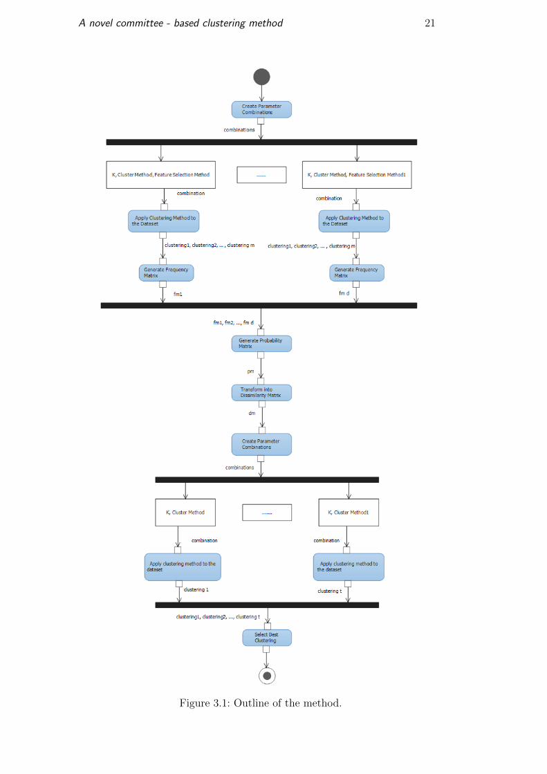
The new method proposed in this chapter for calculating the similarity matrix
is part of the idea of clustering ensemble in unsupervised learning. The method
is comprised of three stages: the first generates the clustering ensemble, the
second combines the results of the multiple scenarios generated and the last
one creates a new partition using the combined data. Figure 3.1 illustrates an
outline of the method as an activity diagram.
The two important characteristics of the method concern the resulting
relevant features and the number of times two objects are assigned to the
same cluster. Our method is independent of the clustering method and feature
selection algorithms. The feature selection methods used are the sequential SFS
and SBS. Each one of theme adopted clustering methods such as K-Means, K-
Medoids (PAM) and Hierarchical Clustering with Average Link.
A novel committee - based clustering method 21
Figure 3.1: Outline of the method.
A novel committee - based clustering method 22
In the first stage, the ensemble is generated by combining the feature
selection methods varying the clustering methods and the number of clusters
k, where k varies from 2 to an input parameter l (by default l = N/2 where
N is the total number of elements). Each possible combination is called a
scenario. A solution belongs to a single scenario and can be defined as a tuple
< k, clm, fsm, rf, silh, fm >, where:
– k is the number of clusters
– clm corresponds to the clustering method used
– fsm is the method of feature selection employed
– rf are the relevant features in the resulting clustering
– silh is the value of the silhouette coefficient
– fm corresponding to the resulting frequency matrix
The frequency matrix (fm) contains in the position (i, j) the mean
silhouette coefficient of the elements i and j, normalized between 0 and 1 (see
Algorithm 2). The silhouette coefficient can be affected by outlier elements in
the cluster. So, to avoid this issue the median was used instead of the mean.
In the second stage, the similarity matrix sim is generated from the multiple
scenarios as shown in Algorithm 1.
Algorithm 1 Algorithm to Generate and Combine the Multiple Scenarios
procedure GenerateScenarios(data,K,CMethods, FSMethods, threshold)sol scen← list()for each k in K do
for each cm in CMethods dofor each fsm in FSMethods do
[rf, clMatrix, sMatrix, silh] ← CreateClustering(data, k, cm,fsm, threshold)
fm ← CreateFrequencyMatrix(clMatrix, sMatrix)scenario← [k, clm, fsm, rf, silh, fm]add scenario to sol scen
sum fm← add the fm from multiple scenariosreturn sim← sum fm/|sol scen|
To quantify the strength of the bind between two objects, the frequency
matrices are filled and finally divided by the number of scenarios, creating the
similarity matrix sim as shown in Algorithm 1, allowing further exploration
of objects and their relationships. The bind between two objects i and j is
defined as the element simi,j and its value ranges from zero to one. So, it
can be interpreted as a probability of element i being in the same cluster as
A novel committee - based clustering method 23
element j. The relation between elements i and j is strong if it is greater than
0.50. This means that they are in the same group in more than half of the
clusterings. The relation is weak when it is lower than 0.20. This means that
they are in the same cluster in less than 20% of the clusterings.
Algorithm 2 Algorithm to Create a Frequency Matrix
procedure CreateFrequencyMatrix(clusteringMatrix, silhouettesMatrix)fm← initialized with 0n← number of rows of clusteringMatrixm← number of columns of clusteringMatrixfor d = 1 to m do
s← silhouettesMatrixd
for each i, j = (1, 1) to (n, n) do
smi,j =si+sj
2+1
2= 1
2∗ (
si+sj2
+ 1) =si+sj+2
4
if clusteringMatrixd[i] == clusteringMatrixd[j] thenfmi,j ← fmi,j + smi,j
return fmm
In the result of a classical clustering algorithm, any two objects can either
be in the same cluster or in different clusters, regardless of their bond. In other
words, an element can have a strong bind with an element outside his cluster
and a weak bind with elements inside it. For instance, when an element is in
the boundaries between a group of clusters, it can be in any one of them, or
when the clustering method has a random component like K-Means.
The main objective of this method is to obtain the similarity matrix
sim and use it to verify the strength of the binds. As part of the third stage,
each element simi,j of this matrix can be transformed using Equation 3-1 or
using Equation 3-2 to be used as the distance matrix dm in other clustering
processes.
dmi,j = 1− simi,j (3-1)
dmi,j = 1−√simi,j (3-2)
Varying the number of clusters and the clustering methods, a new set of
partitions is generated using the dissimilarity matrix dm as distances between
the elements. Notice that here the features are not used to calculate distances
like in the first stage of the method, only the relationships between the
elements. Finally, the partition with the best silhouette coefficient is used to
generate a recommendation of the final clustering and the number of clusters.
Having this in mind, this final recommendation is defined as a tuple
< sim, rfs, fcl, k > where sim is the similarity matrix, rfs are the relevant

A novel committee - based clustering method 24
features, fcl is the final clustering and k is the number of clusters in fcl.
This recommendation is given the initial parameters, namely: a set of cluster
numbers, a set of clustering methods, and a set of feature selection methods.
4Visual Exploration Tools based on the Similarity Matrix
This chapter proposes some visual exploration tools of the similarity matrix,
constructed according to the method proposed in the previous chapter, to
facilitate the understanding of the internal structure of the final clustering.
At the user interface, the user sets a pair < min,max > as a parameter,
named interval threshold or simply threshold, with the following property:
0 ≤ min ≤ max ≤ 1.
The visual tool uses this interval to filter the data in the similarity
matrix, removing all the values lower than min and all the values greater
than max. The visualizations are then focused on analysing the sensibility of
the threshold on the similarity matrix. Filtering the matrix also produces a
clearer representation of the desired data and a better definition of patterns in
the matrix.
In the proposed interface, the screen is composed of four sections (see
Figure 4.1), three of them related to the similarity matrix from different points
of view (heat map, graph and edge bundle) and a fourth section dedicated to
the spatial visualization of the elements (map), in the case of georeferenced
data. Even when showing different points of view, all the sections are related
to allowing users to explore the one which they deem more useful for their
current purposes. In addition, the colors used to represent each cluster serve
as a visual aid to relate the different sections, with the exception of the heat
map, which has its own color scale.
A novel committee - based clustering method 26
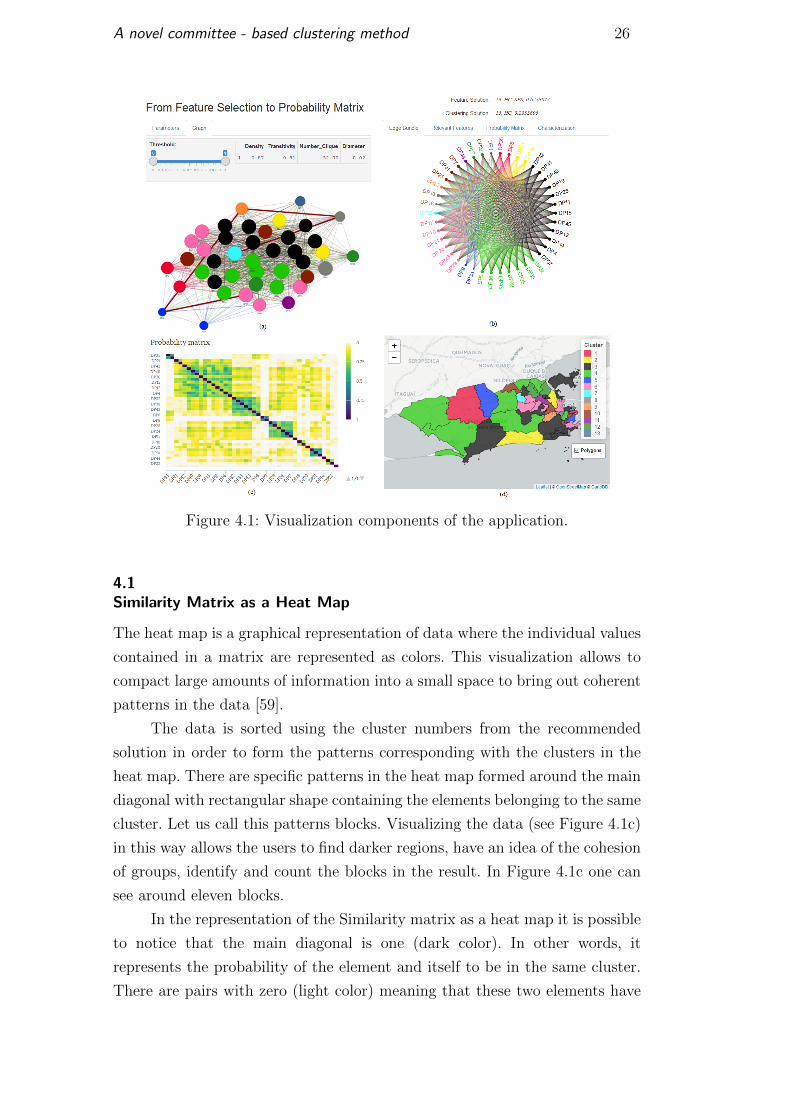
Figure 4.1: Visualization components of the application.
4.1Similarity Matrix as a Heat Map
The heat map is a graphical representation of data where the individual values
contained in a matrix are represented as colors. This visualization allows to
compact large amounts of information into a small space to bring out coherent
patterns in the data [59].
The data is sorted using the cluster numbers from the recommended
solution in order to form the patterns corresponding with the clusters in the
heat map. There are specific patterns in the heat map formed around the main
diagonal with rectangular shape containing the elements belonging to the same
cluster. Let us call this patterns blocks. Visualizing the data (see Figure 4.1c)
in this way allows the users to find darker regions, have an idea of the cohesion
of groups, identify and count the blocks in the result. In Figure 4.1c one can
see around eleven blocks.
In the representation of the Similarity matrix as a heat map it is possible
to notice that the main diagonal is one (dark color). In other words, it
represents the probability of the element and itself to be in the same cluster.
There are pairs with zero (light color) meaning that these two elements have
A novel committee - based clustering method 27
no binds. A continuous color palette going from light to dark has been adopted
to represent the probability of the two elements being on the same cluster.
4.2Similarity Matrix as a Hierarchical Edge Bundling
Hierarchical edge bundling is a flexible and generic method that can be used in
conjunction with existing tree visualization techniques to enable users to choose
the tree visualization that they prefer and to facilitate integration into existing
tools. It reduces visual clutter when dealing with large numbers of adjacency
edges and provides an intuitive and continuous way to control the strength
of bundling. Low bundling strength mainly provides low-level, node-to-node
connectivity information, whereas high bundling strength provides high-level
information as well by implicit visualization of adjacency edges between parent
nodes that are the result of explicit adjacency edges between their respective
child nodes [29].
At first glance, it lets you know the number of items per group. If an
item is selected, users may quickly see the related items (i.e., items that share
an edge with the selected one) and whether they are in the same group or not.
If all the elements with which it is linked are in the same group (and thus
represented in the same color, in our approach), they reinforce the idea that
this group is very cohesive.
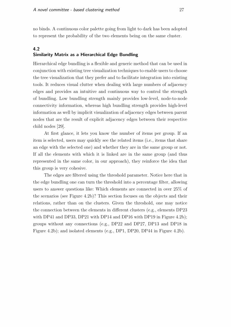
The edges are filtered using the threshold parameter. Notice here that in
the edge bundling one can turn the threshold into a percentage filter, allowing
users to answer questions like: Which elements are connected in over 25% of
the scenarios (see Figure 4.2b)? This section focuses on the objects and their
relations, rather than on the clusters. Given the threshold, one may notice
the connection between the elements in different clusters (e.g., elements DP23
with DP41 and DP33, DP21 with DP14 and DP16 with DP19 in Figure 4.2b);
groups without any connections (e.g., DP22 and DP27, DP13 and DP18 in
Figure 4.2b); and isolated elements (e.g., DP1, DP20, DP44 in Figure 4.2b).
A novel committee - based clustering method 28
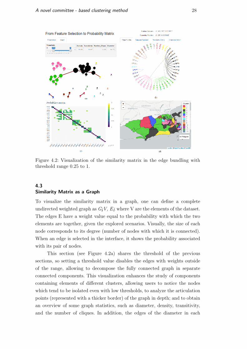
Figure 4.2: Visualization of the similarity matrix in the edge bundling withthreshold range 0.25 to 1.
4.3Similarity Matrix as a Graph
To visualize the similarity matrix in a graph, one can define a complete
undirected weighted graph as G¡V, E¿ where V are the elements of the dataset.
The edges E have a weight value equal to the probability with which the two
elements are together, given the explored scenarios. Visually, the size of each
node corresponds to its degree (number of nodes with which it is connected).
When an edge is selected in the interface, it shows the probability associated
with its pair of nodes.
This section (see Figure 4.2a) shares the threshold of the previous
sections, so setting a threshold value disables the edges with weights outside
of the range, allowing to decompose the fully connected graph in separate
connected components. This visualization enhances the study of components
containing elements of different clusters, allowing users to notice the nodes
which tend to be isolated even with low thresholds, to analyze the articulation
points (represented with a thicker border) of the graph in depth; and to obtain
an overview of some graph statistics, such as diameter, density, transitivity,
and the number of cliques. In addition, the edges of the diameter in each
A novel committee - based clustering method 29
connected component are presented in a different way, particularity, edge in
red color.
4.4Clustering Solution in Map
Georeferenced objects, such as schools, police stations, neighborhoods, cities
and countries, are visualized in a map to easily analyze whether adjacent ele-
ments belong to the same cluster; to compare regions; to uncover a geographic
pattern of the data; to locate which regions should be further analyzed by
domain experts (see Figure 4.1d); and to investigate why some regions have
unexpected behaviours. When one clicks on a region, a pop-up with some data
as region name about it appears.
4.5Discussion
The visualizations adopted in this approach support the descriptive analysis
of the results. Combining different points of view, users can achieve more
sophisticated results and explore the data more efficiently. Some of the most
interesting facts about the data can be in one articulation point or an outlier,
and conventional exploration of the data can cause users to miss some of these
key details, which are relevant qualitative information that can explain or help
to understand a problem. Enhancing the user experience not only is a good
practice, but it also reduces the time spent on the descriptive analysis of the
dataset in a research project.
5Experiments and Results
This chapter presents the experiments and the results obtained. To evaluate
the performance of the method (Section 5.1), first it presents a comparison
between several clustering methods like K-Means, PAM, HC with Average
Link and the proposed method (subsection 5.1.1), and then it shows another
comparison between clustering methods based on ensemble techniques and
our method (subsection 5.1.2). The comparison measures the quality of the
resulting clusters using normalized mutual information. Section 5.2 shows
several experiments applying our method in two real life datasets. The first
one is about the crime data in the State of Rio de Janeiro (subsection 5.2.1)
and the second one is about the Human Development Index in the year 2014
(subsection 5.2.2). Section 5.3 concludes this chapter with a discussion about
the results.
5.1Performances of our Method
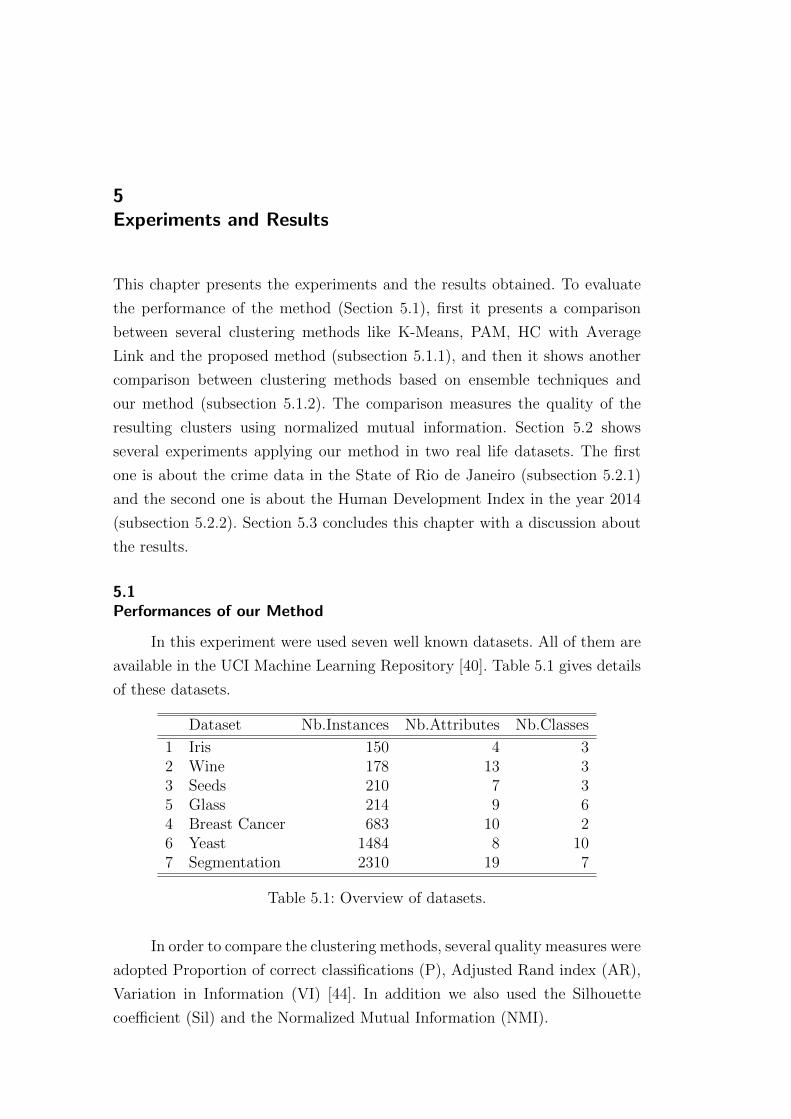
In this experiment were used seven well known datasets. All of them are
available in the UCI Machine Learning Repository [40]. Table 5.1 gives details
of these datasets.
Dataset Nb.Instances Nb.Attributes Nb.Classes
1 Iris 150 4 32 Wine 178 13 33 Seeds 210 7 35 Glass 214 9 64 Breast Cancer 683 10 26 Yeast 1484 8 107 Segmentation 2310 19 7
Table 5.1: Overview of datasets.
In order to compare the clustering methods, several quality measures were
adopted Proportion of correct classifications (P), Adjusted Rand index (AR),
Variation in Information (VI) [44]. In addition we also used the Silhouette
coefficient (Sil) and the Normalized Mutual Information (NMI).
A novel committee - based clustering method 31
The clustering methods used are available in R [1], K-Means and HC-
AL from the stats package, PAM from cluster package; the measures
Silhouette from cluster package, P, AR and VI from MixSim package and,
finally, NMI using the infotheo package.
The clustering methods used were divided in two groups: first, individual
clustering algorithms and second a group based on ensemble clustering.
5.1.1Comparison with individual clustering methods
The individual clustering method used in this experiment are K-Means, PAM
and HC with Average Link and the results are given in Table 5.2. In bold
are highlighted the better results of each method according to Proportion of
correct classifications (P) and Normalized Mutual Information (NMI).
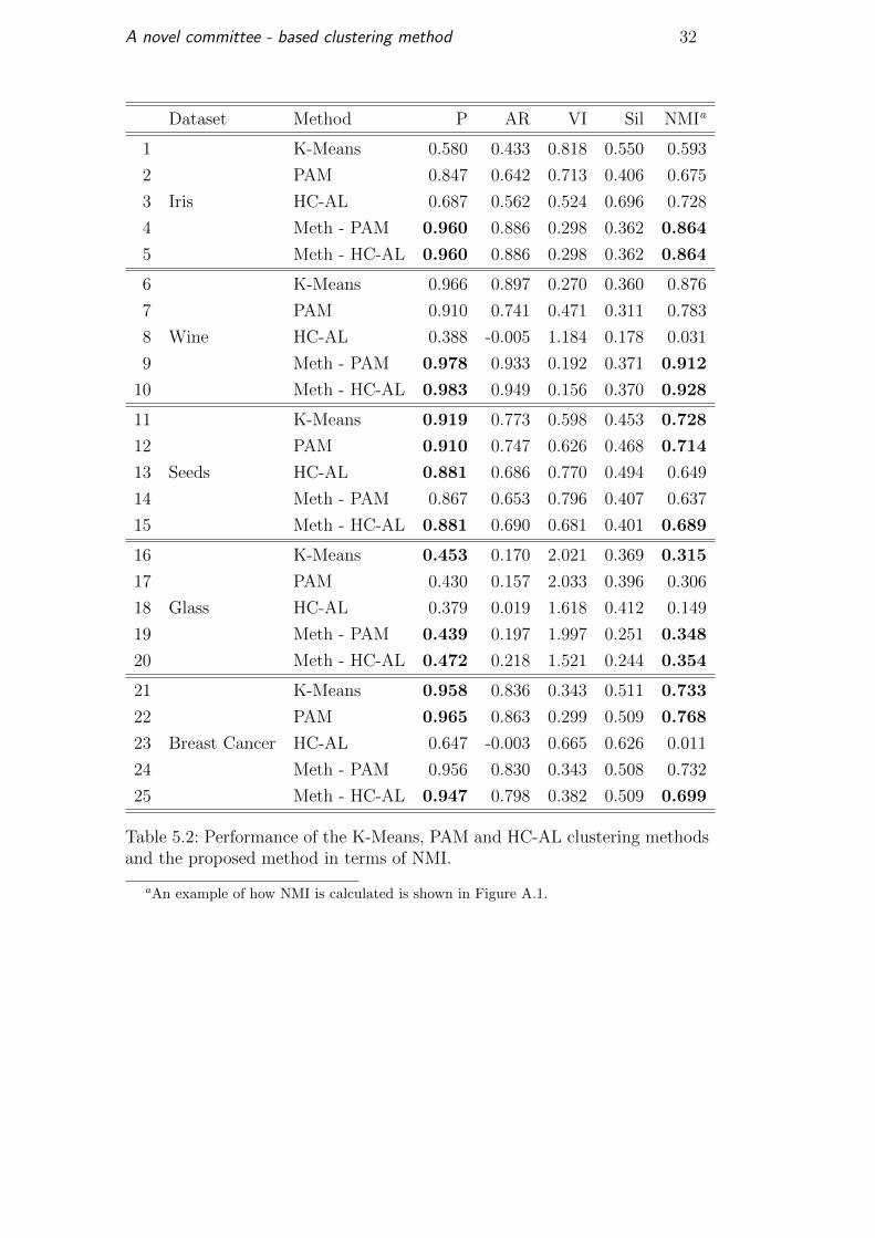
A novel committee - based clustering method 32
Dataset Method P AR VI Sil NMIa
1 K-Means 0.580 0.433 0.818 0.550 0.593
2 PAM 0.847 0.642 0.713 0.406 0.675
3 Iris HC-AL 0.687 0.562 0.524 0.696 0.728
4 Meth - PAM 0.960 0.886 0.298 0.362 0.864
5 Meth - HC-AL 0.960 0.886 0.298 0.362 0.864
6 K-Means 0.966 0.897 0.270 0.360 0.876
7 PAM 0.910 0.741 0.471 0.311 0.783
8 Wine HC-AL 0.388 -0.005 1.184 0.178 0.031
9 Meth - PAM 0.978 0.933 0.192 0.371 0.912
10 Meth - HC-AL 0.983 0.949 0.156 0.370 0.928
11 K-Means 0.919 0.773 0.598 0.453 0.728
12 PAM 0.910 0.747 0.626 0.468 0.714
13 Seeds HC-AL 0.881 0.686 0.770 0.494 0.649
14 Meth - PAM 0.867 0.653 0.796 0.407 0.637
15 Meth - HC-AL 0.881 0.690 0.681 0.401 0.689
16 K-Means 0.453 0.170 2.021 0.369 0.315
17 PAM 0.430 0.157 2.033 0.396 0.306
18 Glass HC-AL 0.379 0.019 1.618 0.412 0.149
19 Meth - PAM 0.439 0.197 1.997 0.251 0.348
20 Meth - HC-AL 0.472 0.218 1.521 0.244 0.354
21 K-Means 0.958 0.836 0.343 0.511 0.733
22 PAM 0.965 0.863 0.299 0.509 0.768
23 Breast Cancer HC-AL 0.647 -0.003 0.665 0.626 0.011
24 Meth - PAM 0.956 0.830 0.343 0.508 0.732
25 Meth - HC-AL 0.947 0.798 0.382 0.509 0.699
Table 5.2: Performance of the K-Means, PAM and HC-AL clustering methodsand the proposed method in terms of NMI.
aAn example of how NMI is calculated is shown in Figure A.1.
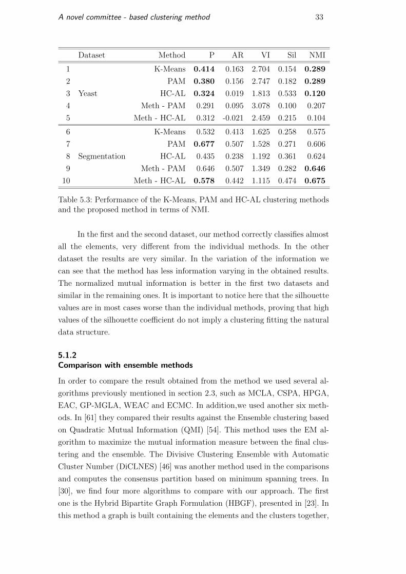
A novel committee - based clustering method 33
Dataset Method P AR VI Sil NMI
1 K-Means 0.414 0.163 2.704 0.154 0.289
2 PAM 0.380 0.156 2.747 0.182 0.289
3 Yeast HC-AL 0.324 0.019 1.813 0.533 0.120
4 Meth - PAM 0.291 0.095 3.078 0.100 0.207
5 Meth - HC-AL 0.312 -0.021 2.459 0.215 0.104
6 K-Means 0.532 0.413 1.625 0.258 0.575
7 PAM 0.677 0.507 1.528 0.271 0.606
8 Segmentation HC-AL 0.435 0.238 1.192 0.361 0.624
9 Meth - PAM 0.646 0.507 1.349 0.282 0.646
10 Meth - HC-AL 0.578 0.442 1.115 0.474 0.675
Table 5.3: Performance of the K-Means, PAM and HC-AL clustering methodsand the proposed method in terms of NMI.
In the first and the second dataset, our method correctly classifies almost
all the elements, very different from the individual methods. In the other
dataset the results are very similar. In the variation of the information we
can see that the method has less information varying in the obtained results.
The normalized mutual information is better in the first two datasets and
similar in the remaining ones. It is important to notice here that the silhouette
values are in most cases worse than the individual methods, proving that high
values of the silhouette coefficient do not imply a clustering fitting the natural
data structure.
5.1.2Comparison with ensemble methods
In order to compare the result obtained from the method we used several al-
gorithms previously mentioned in section 2.3, such as MCLA, CSPA, HPGA,
EAC, GP-MGLA, WEAC and ECMC. In addition,we used another six meth-
ods. In [61] they compared their results against the Ensemble clustering based
on Quadratic Mutual Information (QMI) [54]. This method uses the EM al-
gorithm to maximize the mutual information measure between the final clus-
tering and the ensemble. The Divisive Clustering Ensemble with Automatic
Cluster Number (DiCLNES) [46] was another method used in the comparisons
and computes the consensus partition based on minimum spanning trees. In
[30], we find four more algorithms to compare with our approach. The first
one is the Hybrid Bipartite Graph Formulation (HBGF), presented in [23]. In
this method a graph is built containing the elements and the clusters together,
A novel committee - based clustering method 34
the bipartite graph is created with edges between elements and clusters. The
second is the Weighted Consensus Clustering (WCC) [39]. This method assigns
weights to the ensemble clusterings to unbalance and adapt their influence in
the final solution. The third is SimRank Similarity Based Method (SRS) [31],
whith proposes an analysis of the neighborhood of the elements, following the
principle that two elements are similar if their respective neighbors are similar
too. The last one is the Weighted Connected Triple Method (WCT) [32]; this
method builds a link network model from the ensemble in order to compute
their similarity and finally refine the similarity to reach the consensus clus-
tering. In the EAC, WEAC, ECMC, SRS and WCT there were used three
variants of the agglomerative clustering (AL, CL, and SL).
The datasets used in the comparison are well known in the scientific
community and several previous work shows the resulted measures on them.
The other methods results are based on the values of the rows with NMI from
Table III in [61] and the column True-k from Table 6 in [30]. These results
are compared with our method in Tables 5.4 and 5.5 respectively. In bold are
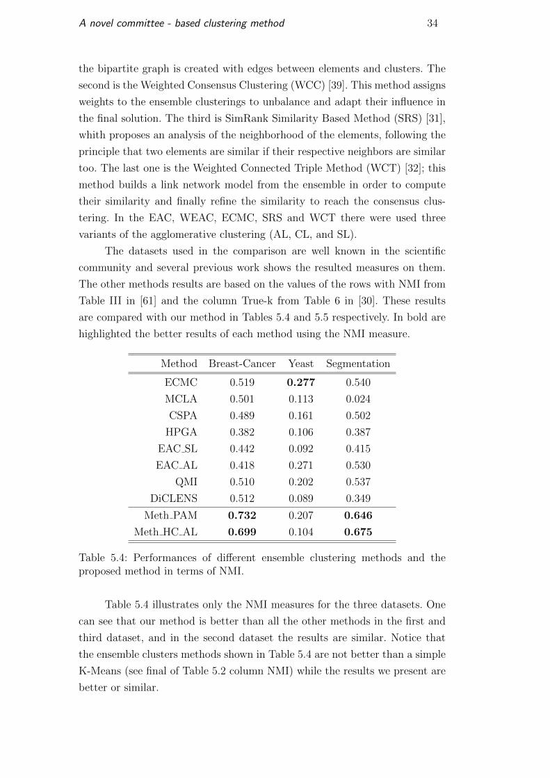
highlighted the better results of each method using the NMI measure.
Method Breast-Cancer Yeast Segmentation
ECMC 0.519 0.277 0.540
MCLA 0.501 0.113 0.024
CSPA 0.489 0.161 0.502
HPGA 0.382 0.106 0.387
EAC SL 0.442 0.092 0.415
EAC AL 0.418 0.271 0.530
QMI 0.510 0.202 0.537
DiCLENS 0.512 0.089 0.349
Meth PAM 0.732 0.207 0.646
Meth HC AL 0.699 0.104 0.675
Table 5.4: Performances of different ensemble clustering methods and theproposed method in terms of NMI.
Table 5.4 illustrates only the NMI measures for the three datasets. One
can see that our method is better than all the other methods in the first and
third dataset, and in the second dataset the results are similar. Notice that
the ensemble clusters methods shown in Table 5.4 are not better than a simple
K-Means (see final of Table 5.2 column NMI) while the results we present are
better or similar.
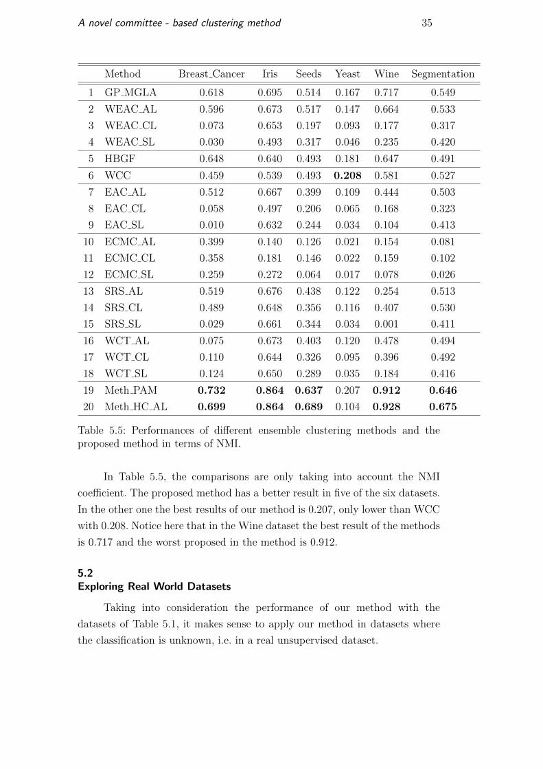
A novel committee - based clustering method 35
Method Breast Cancer Iris Seeds Yeast Wine Segmentation
1 GP MGLA 0.618 0.695 0.514 0.167 0.717 0.549
2 WEAC AL 0.596 0.673 0.517 0.147 0.664 0.533
3 WEAC CL 0.073 0.653 0.197 0.093 0.177 0.317
4 WEAC SL 0.030 0.493 0.317 0.046 0.235 0.420
5 HBGF 0.648 0.640 0.493 0.181 0.647 0.491
6 WCC 0.459 0.539 0.493 0.208 0.581 0.527
7 EAC AL 0.512 0.667 0.399 0.109 0.444 0.503
8 EAC CL 0.058 0.497 0.206 0.065 0.168 0.323
9 EAC SL 0.010 0.632 0.244 0.034 0.104 0.413
10 ECMC AL 0.399 0.140 0.126 0.021 0.154 0.081
11 ECMC CL 0.358 0.181 0.146 0.022 0.159 0.102
12 ECMC SL 0.259 0.272 0.064 0.017 0.078 0.026
13 SRS AL 0.519 0.676 0.438 0.122 0.254 0.513
14 SRS CL 0.489 0.648 0.356 0.116 0.407 0.530
15 SRS SL 0.029 0.661 0.344 0.034 0.001 0.411
16 WCT AL 0.075 0.673 0.403 0.120 0.478 0.494
17 WCT CL 0.110 0.644 0.326 0.095 0.396 0.492
18 WCT SL 0.124 0.650 0.289 0.035 0.184 0.416
19 Meth PAM 0.732 0.864 0.637 0.207 0.912 0.646
20 Meth HC AL 0.699 0.864 0.689 0.104 0.928 0.675
Table 5.5: Performances of different ensemble clustering methods and theproposed method in terms of NMI.
In Table 5.5, the comparisons are only taking into account the NMI
coefficient. The proposed method has a better result in five of the six datasets.
In the other one the best results of our method is 0.207, only lower than WCC
with 0.208. Notice here that in the Wine dataset the best result of the methods
is 0.717 and the worst proposed in the method is 0.912.
5.2Exploring Real World Datasets
Taking into consideration the performance of our method with the
datasets of Table 5.1, it makes sense to apply our method in datasets where
the classification is unknown, i.e. in a real unsupervised dataset.
A novel committee - based clustering method 36
5.2.1Exploring the CrimesRJ Dataset
In Rio de Janeiro, the public access to data is not straightforward. The Public
Safety Institute (ISP) publishes monthly spreadsheets since 2002, orginized
by public safety area (Areas de Seguranca Publica – AISPs) [2]. An AISP
is a territorial subdivision for administrative purposes. The state is divided
in 41 AISPs, and each one is composed of a distinct number of DPs, where
crime occurrences are recorded. Therefore, a monthly report is composed of 41
spreadsheets, and each spreadsheet includes the total number of occurrences
for 39 kinds of crime for each DP that comprises the AISP.
To exemplify the difficulty in obtaining data, in a temporal analysis of a
certain type of crime it would be necessary to download all the monthly files,
almost 150 at the time of this study, to locate in each file the AISP, the DP,
the type of crime, and only then collect the desired information. This way of
publishing public data can satisfy a legal obligation, but it certainly does not
serve the society in a convenient way.
The process of gathering data comprises several activities:
1. processing criminality data from ISP spreadsheets;
2. gathering spatial data from ISP and IBGE [3];
3. establishing the correspondence of the spatial data from each source; and
4. associating demographic data (IBGE) to the geographic areas.
The monthly spreadsheets were obtained from the ISP website, which
does not have an area for direct access (e.g., FTP). We developed an algorithm
that scrapes the ISP web page, identifies the name of the data files and down-
loads them to local storage. By executing this program we can obtain all the
available spreadsheets. The data in all spreadsheets were interpreted, aggreg-
ated, and stored in a single file without losing information. This operation was
not straightforward, because those monthly spreadsheets present variations in
structure and in the identification of type of crime, which require a series of
adjustments. For instance, to identify the type of crime we built a dictionary
to relate a standard noun to its diverse aliases adopted over the years.
All contextualization of data on criminality depends on several social and
economic factors, which interact and change according to their location, city,
neighborhood, etc. Therefore the delimitation of the territory to which crimes
are associated is fundamental to the analyses. In the data at hand, the most
fine-grained territory delimitation is the DP, i.e., the most detailed information
is the number of occurrences of each type of crime recorded at each DP. In
A novel committee - based clustering method 37
May 2015, ISP made available in its website the geographic boundaries of the
DPs in digital format (as shapefiles). With these official digital maps one can
truly recognize the boundaries of each DP. In theory, with that information
it would be possible to relate those territories with the information about the
population (associated to territories called census sectors by IBGE) and build
a socioeconomic database to enrich the analyses. The apparently simple idea
of aggregating the census sectors with the DP areas proved to be complicated.
The digital DP maps did not coincide with the census sectors boundaries,
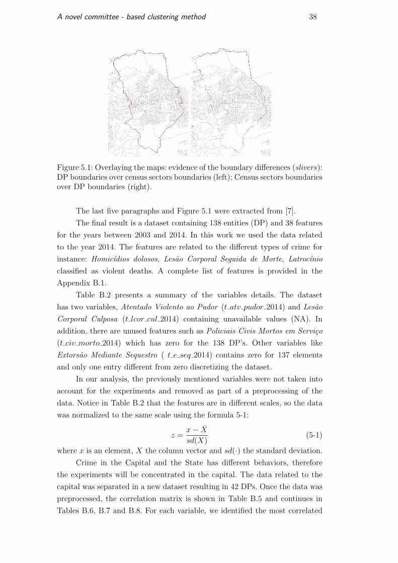
making it impossible to automatically relate or aggregate the data. Figure 5.1
illustrates the problem. The figure on the left shows the boundaries of a DP
(in red) over the boundaries of census sectors in the city of Rio de Janeiro
in 2010, and figure on the right shows the boundaries of the census sectors
over the DP boundaries. Notice that some red lines still appear in the right
figure, indicating that on those locations the boundaries do not coincide. This
generates a large number of small polygons (slivers) in the overlays. An even
coarser error can be observed on the top of both figures, where a region of a
DP in the capital region is outside the boundaries of the city itself. To solve
this problem, we developed an algorithm to automatically correct distortions
and associate the census data to each DP. This algorithm detects all sectors
under the boundaries of a DP area and alters these boundaries according to
the following criteria: If the sector belongs to the same city as the DP and
if the area that exceeds the DP boundaries is smaller than the internal area,
then the DP area is extended to include the sector; otherwise, the DP area
is shrunk to exclude the entire sector. In these adjustments, the percentage
of the included or excluded area was always less than 5%. The algorithm was
executed for the entire state of Rio de Janeiro, in the 28, 318 census sectors,
generating the correction of the polygons of the 138 DPs and a list of census
sectors corresponding to each DP.
Adjusting the spatial regions for their boundaries to coincide enabled
querying the IBGE databases and obtaining the populations of each DP area
in 2000 and 2010. This in turn allowed us to estimate the population of each DP
from 2003 to 2014. The estimated populations were considered as a reference
and used as a constant for every month of the corresponding year. As there
is no information of the DP boundaries for all years, the boundaries made
available in 2015 were used for the entire period of study.
A novel committee - based clustering method 38
Figure 5.1: Overlaying the maps: evidence of the boundary differences (slivers):DP boundaries over census sectors boundaries (left); Census sectors boundariesover DP boundaries (right).
The last five paragraphs and Figure 5.1 were extracted from [7].
The final result is a dataset containing 138 entities (DP) and 38 features
for the years between 2003 and 2014. In this work we used the data related
to the year 2014. The features are related to the different types of crime for
instance: Homicıdios dolosos, Lesao Corporal Seguida de Morte, Latrocınio
classified as violent deaths. A complete list of features is provided in the
Appendix B.1.
Table B.2 presents a summary of the variables details. The dataset
has two variables, Atentado Violento ao Pudor (t atv pudor 2014) and Lesao
Corporal Culposa (t lcor cul 2014) containing unavailable values (NA). In
addition, there are unused features such as Policiais Civis Mortos em Servico
(t civ morto 2014) which has zero for the 138 DP’s. Other variables like
Extorsao Mediante Sequestro ( t e seq 2014) contains zero for 137 elements
and only one entry different from zero discretizing the dataset.
In our analysis, the previously mentioned variables were not taken into
account for the experiments and removed as part of a preprocessing of the
data. Notice in Table B.2 that the features are in different scales, so the data
was normalized to the same scale using the formula 5-1:
z =x− X
sd(X)(5-1)
where x is an element, X the column vector and sd(·) the standard deviation.
Crime in the Capital and the State has different behaviors, therefore
the experiments will be concentrated in the capital. The data related to the
capital was separated in a new dataset resulting in 42 DPs. Once the data was
preprocessed, the correlation matrix is shown in Table B.5 and continues in
Tables B.6, B.7 and B.8. For each variable, we identified the most correlated
A novel committee - based clustering method 39
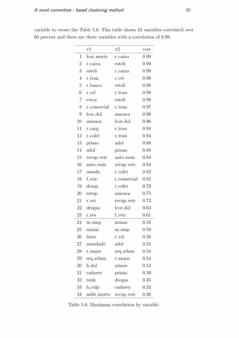
variable to create the Table 5.6. This table shows 23 variables correlated over
60 percent and there are three variables with a correlation of 0.99.
v1 v2 corr
1 lcor morte r caixa 0.99
2 r caixa esteli 0.99
3 esteli r caixa 0.99
4 r tran r cel 0.98
5 r banco esteli 0.98
6 r cel r tran 0.98
7 extor esteli 0.98
8 r comercial r tran 0.97
9 lcor dol ameaca 0.96
10 ameaca lcor dol 0.96
11 r carg r tran 0.94
12 r colet r tran 0.94
13 prisao adol 0.88
14 adol prisao 0.88
15 recup veic auto resis 0.84
16 auto resis recup veic 0.84
17 ossada r colet 0.82
18 f veic r comercial 0.82
19 desap r colet 0.79
20 estup ameaca 0.75
21 r vei recup veic 0.72
22 drogas lcor dol 0.63
23 r res f veic 0.61
24 m susp armas 0.59
25 armas m susp 0.59
26 latro r vei 0.56
27 mandado adol 0.55
28 r saque seq relam 0.54
29 seq relam r saque 0.54
30 h dol armas 0.52
31 cadaver prisao 0.39
32 tenh drogas 0.35
33 h culp cadaver 0.32
34 milit morto recup veic 0.30
Table 5.6: Maximum correlation by variable.
A novel committee - based clustering method 40
Capital
In order to have an idea of the dataset we are dealing with, we devised an
experiment that selects a random subset with 3 to 12 features, the PAM is
set as the clustering method and the silhouette as the quality measure. We
run 100000 simulations with 4, 7 and 10 groups. Table 5.7 shows the results.
In addition, for each number of clusters, we applied the SFS and the SBS
methods. The results are summarized in Table 5.8.
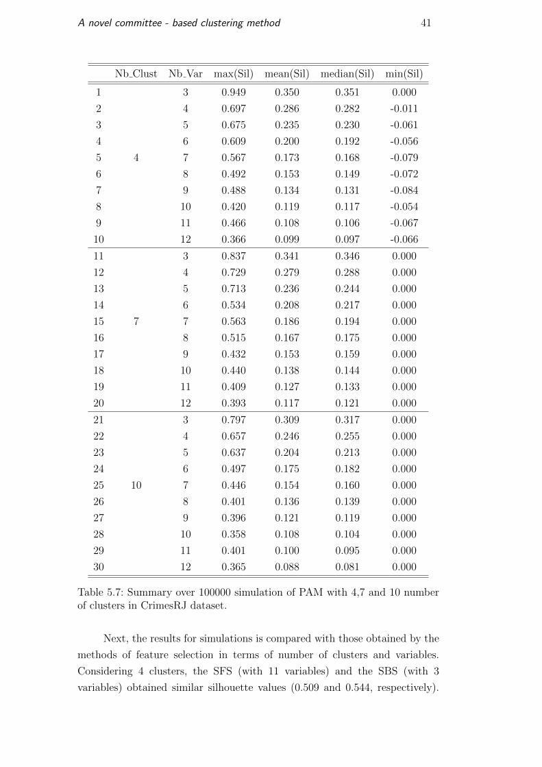
Observing the column max(Sil) of Table 5.7, one can see that when the
number of variables is increased, there is a tendency to reduce the silhouette
coefficient. Also, the mean and median have similar values; therefore the
silhouette distribution resulted from the simulations is symmetric. Notice that
there are no values near to −1, so there are no extremely bad clusterings.
A novel committee - based clustering method 41
Nb Clust Nb Var max(Sil) mean(Sil) median(Sil) min(Sil)
1 3 0.949 0.350 0.351 0.000
2 4 0.697 0.286 0.282 -0.011
3 5 0.675 0.235 0.230 -0.061
4 6 0.609 0.200 0.192 -0.056
5 4 7 0.567 0.173 0.168 -0.079
6 8 0.492 0.153 0.149 -0.072
7 9 0.488 0.134 0.131 -0.084
8 10 0.420 0.119 0.117 -0.054
9 11 0.466 0.108 0.106 -0.067
10 12 0.366 0.099 0.097 -0.066
11 3 0.837 0.341 0.346 0.000
12 4 0.729 0.279 0.288 0.000
13 5 0.713 0.236 0.244 0.000
14 6 0.534 0.208 0.217 0.000
15 7 7 0.563 0.186 0.194 0.000
16 8 0.515 0.167 0.175 0.000
17 9 0.432 0.153 0.159 0.000
18 10 0.440 0.138 0.144 0.000
19 11 0.409 0.127 0.133 0.000
20 12 0.393 0.117 0.121 0.000
21 3 0.797 0.309 0.317 0.000
22 4 0.657 0.246 0.255 0.000
23 5 0.637 0.204 0.213 0.000
24 6 0.497 0.175 0.182 0.000
25 10 7 0.446 0.154 0.160 0.000
26 8 0.401 0.136 0.139 0.000
27 9 0.396 0.121 0.119 0.000
28 10 0.358 0.108 0.104 0.000
29 11 0.401 0.100 0.095 0.000
30 12 0.365 0.088 0.081 0.000
Table 5.7: Summary over 100000 simulation of PAM with 4,7 and 10 numberof clusters in CrimesRJ dataset.
Next, the results for simulations is compared with those obtained by the
methods of feature selection in terms of number of clusters and variables.
Considering 4 clusters, the SFS (with 11 variables) and the SBS (with 3
variables) obtained similar silhouette values (0.509 and 0.544, respectively).
A novel committee - based clustering method 42
Considering 7 clusters, the simulation obtained better results with a silhouette
of 0.713 for the SBS method and 0.589 for the SFS.
FSM Nb Clust Sil Nb Var InfoVar
1 4 0.509 11 8, 22, 36, 2, 18, 25, 17, 27, 23, 19, 31
2 SFS 7 0.589 5 13, 22, 36, 2, 17
3 10 0.514 8 13, 22, 36, 24, 18, 25, 2, 23
4 4 0.544 3 24, 27, 34
5 SBS 7 0.830 1 13
6 10 0.525 2 13, 28
Table 5.8: Summary of SFS and SBS with PAM and 0.5 of threshold with 4,7 and 10 number of clusters in the CrimesRJ dataset.
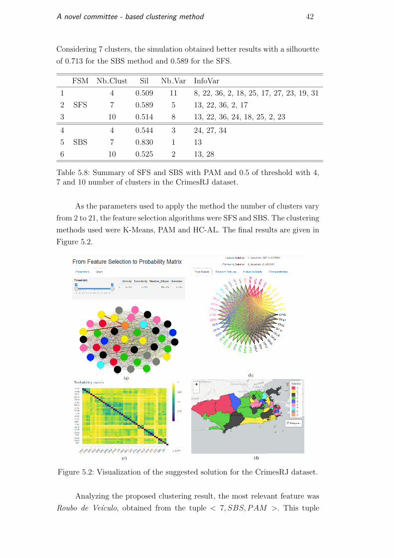
As the parameters used to apply the method the number of clusters vary
from 2 to 21, the feature selection algorithms were SFS and SBS. The clustering
methods used were K-Means, PAM and HC-AL. The final results are given in
Figure 5.2.
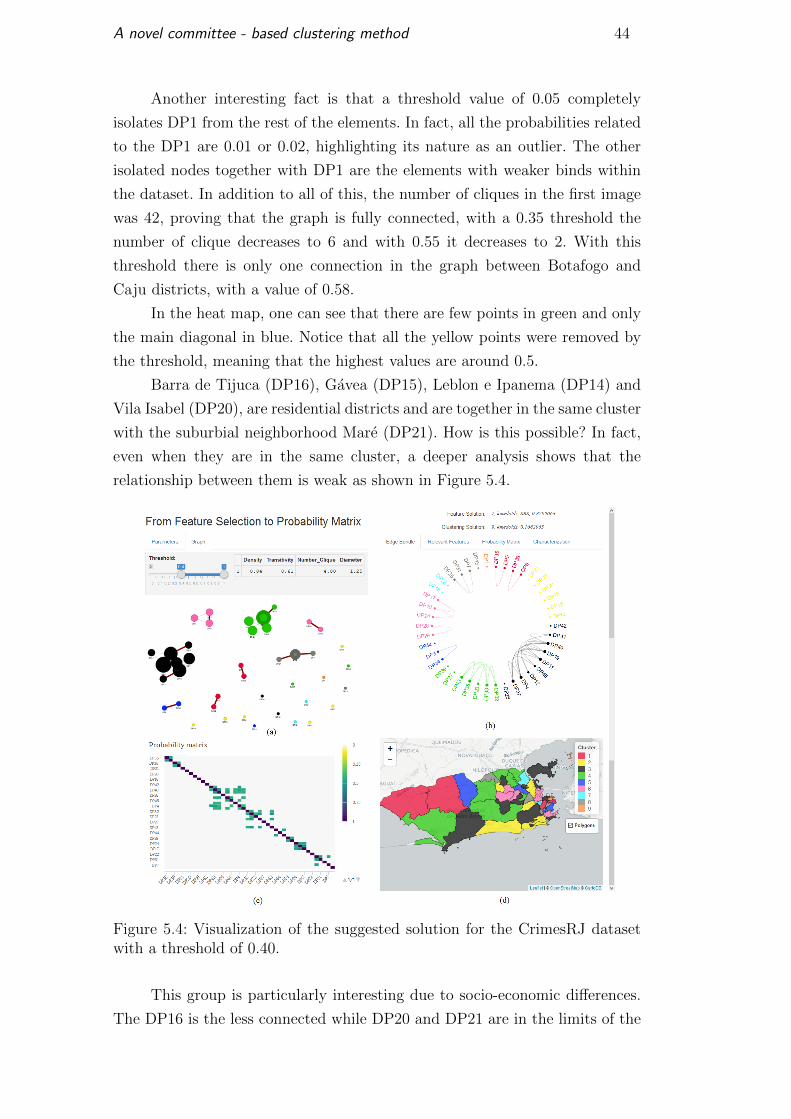
Figure 5.2: Visualization of the suggested solution for the CrimesRJ dataset.
Analyzing the proposed clustering result, the most relevant feature was
Roubo de Veıculo, obtained from the tuple < 7, SBS, PAM >. This tuple
A novel committee - based clustering method 43
obtained the highest silhouette value, around 0.8. Using the similarity matrix,
our method proposed 9 clusters with a silhouette around 0.17 and using PAM.
In the map it is possible to identify a black cluster formed with Rocinha
(DP11), Complexo Alamao (DP45), some districts of the Ilha do Governador
(DP37), part of Copacabana, Leme (DP12), part of Centro (DP4), Pechincha
(DP41), Alto de Boa Vista (DP19), Coelho Neto (DP40) and Recreio (DP42).
Isolated in orange is the DP1 in Centro. This DP is an outlier because
to the variables in this area are affected by the large flow of people, and there
is no way to calculate or estimate this flow.
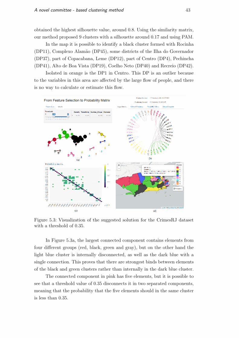
Figure 5.3: Visualization of the suggested solution for the CrimesRJ datasetwith a threshold of 0.35.
In Figure 5.3a, the largest connected component contains elements from
four different groups (red, black, green and gray), but on the other hand the
light blue cluster is internally disconnected, as well as the dark blue with a
single connection. This proves that there are strongest binds between elements
of the black and green clusters rather than internally in the dark blue cluster.
The connected component in pink has five elements, but it is possible to
see that a threshold value of 0.35 disconnects it in two separated components,
meaning that the probability that the five elements should in the same cluster
is less than 0.35.
A novel committee - based clustering method 44
Another interesting fact is that a threshold value of 0.05 completely
isolates DP1 from the rest of the elements. In fact, all the probabilities related
to the DP1 are 0.01 or 0.02, highlighting its nature as an outlier. The other
isolated nodes together with DP1 are the elements with weaker binds within
the dataset. In addition to all of this, the number of cliques in the first image
was 42, proving that the graph is fully connected, with a 0.35 threshold the
number of clique decreases to 6 and with 0.55 it decreases to 2. With this
threshold there is only one connection in the graph between Botafogo and
Caju districts, with a value of 0.58.
In the heat map, one can see that there are few points in green and only
the main diagonal in blue. Notice that all the yellow points were removed by
the threshold, meaning that the highest values are around 0.5.
Barra de Tijuca (DP16), Gavea (DP15), Leblon e Ipanema (DP14) and
Vila Isabel (DP20), are residential districts and are together in the same cluster
with the suburbial neighborhood Mare (DP21). How is this possible? In fact,
even when they are in the same cluster, a deeper analysis shows that the
relationship between them is weak as shown in Figure 5.4.
Figure 5.4: Visualization of the suggested solution for the CrimesRJ datasetwith a threshold of 0.40.
This group is particularly interesting due to socio-economic differences.
The DP16 is the less connected while DP20 and DP21 are in the limits of the
A novel committee - based clustering method 45
clustering. In Barra da Tijuca there are few street shops, long avenues and
it is uncommon to see people walking on the streets. This DP has the lower
records of the group, who knows if it is due to urban planning characteristics?
Mare, even though it is a suburb, contains UPP (Pacifying Police Unit)[4] and
has similar results with the rest of the cluster as shown, in Figure B.1.
The yellow cluster is fully disconnected, with a threshold of 0.4. Also
with this threshold disappear all the connections between elements in different
clusters and there is still a strong connectivity in the black and green clusters.
The black cluster still has no articulation points and the green cluster has
only one but has a clique number of 4, the biggest in the whole graph. On the
other hand, the yellow, gray, dark blue and red have connections lower than
the number on elements, so these are sparsely connected components.
Finally, it is important to say that the most important variable is the
Roubo de Veiculo and there are subgroups with very similar characteristics
that deserve a qualitative analysis and a more detailed study of the similarity
reasons.
The other experiment is related to the location of the AISPs (Integrated
Area of Public Security). The AISPs are administrative areas that fit with
the areas in charge of the Battalions of Military Police, without taking into
account the socio-economic or crime related characteristics of the region.
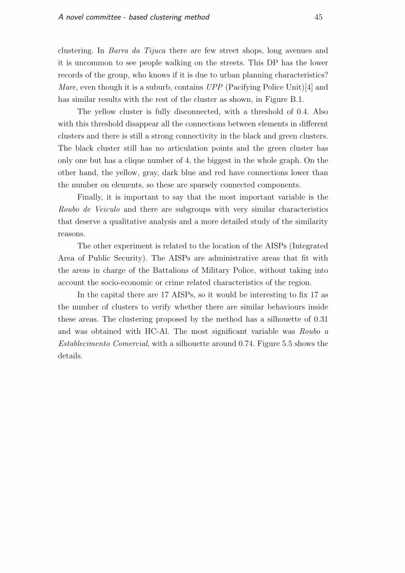
In the capital there are 17 AISPs, so it would be interesting to fix 17 as
the number of clusters to verify whether there are similar behaviours inside
these areas. The clustering proposed by the method has a silhouette of 0.31
and was obtained with HC-Al. The most significant variable was Roubo a
Establecimento Comercial, with a silhouette around 0.74. Figure 5.5 shows the
details.
A novel committee - based clustering method 46
Figure 5.5: Visualization of the suggested solution for 17 clusters in theCrimesRJ dataset.
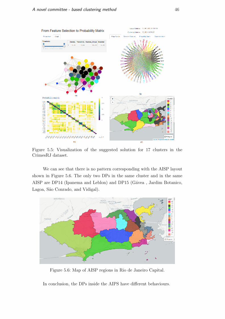
We can see that there is no pattern corresponding with the AISP layout
shown in Figure 5.6. The only two DPs in the same cluster and in the same
AISP are DP14 (Ipanema and Leblon) and DP15 (Gavea , Jardim Botanico,
Lagoa, Sao Conrado, and Vidigal).
Figure 5.6: Map of AISP regions in Rio de Janeiro Capital.
In conclusion, the DPs inside the AIPS have different behaviours.
A novel committee - based clustering method 47
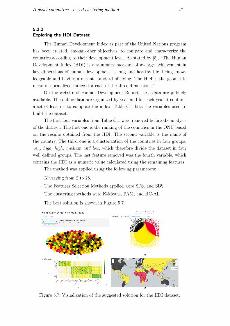
5.2.2Exploring the HDI Dataset
The Human Development Index as part of the United Nations program
has been created, among other objectives, to compare and characterize the
countries according to their development level. As stated by [5], “The Human
Development Index (HDI) is a summary measure of average achievement in
key dimensions of human development: a long and healthy life, being know-
ledgeable and having a decent standard of living. The HDI is the geometric
mean of normalized indices for each of the three dimensions.”
On the website of Human Development Report these data are publicly
available. The online data are organized by year and for each year it contains
a set of features to compute the index. Table C.1 lists the variables used to
build the dataset.
The first four variables from Table C.1 were removed before the analysis
of the dataset. The first one is the ranking of the countries in the ONU based
on the results obtained from the HDI. The second variable is the name of
the country. The third one is a clusterization of the countries in four groups:
very high, high, medium and low, which therefore divide the dataset in four
well defined groups. The last feature removed was the fourth variable, which
contains the HDI as a numeric value calculated using the remaining features.
The method was applied using the following parameters:
– K varying from 2 to 28.
– The Features Selection Methods applied were SFS, and SBS.
– The clustering methods were K-Means, PAM, and HC-AL.
The best solution is shown in Figure 5.7.
Figure 5.7: Visualization of the suggested solution for the HDI dataset.
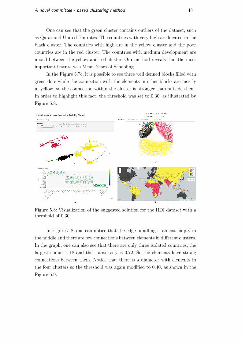
A novel committee - based clustering method 48
One can see that the green cluster contains outliers of the dataset, such
as Qatar and United Emirates. The countries with very high are located in the
black cluster. The countries with high are in the yellow cluster and the poor
countries are in the red cluster. The countries with medium development are
mixed between the yellow and red cluster. Our method reveals that the most
important feature was Mean Years of Schooling.
In the Figure 5.7c, it is possible to see three well defined blocks filled with
green dots while the connection with the elements in other blocks are mostly
in yellow, so the connection within the cluster is stronger than outside them.
In order to highlight this fact, the threshold was set to 0.30, as illustrated by
Figure 5.8.
Figure 5.8: Visualization of the suggested solution for the HDI dataset with athreshold of 0.30.
In Figure 5.8, one can notice that the edge bundling is almost empty in
the middle and there are few connections between elements in different clusters.
In the graph, one can also see that there are only three isolated countries, the
largest clique is 18 and the transitivity is 0.72. So the elements have strong
connections between them. Notice that there is a diameter with elements in
the four clusters so the threshold was again modified to 0.40, as shown in the
Figure 5.9.
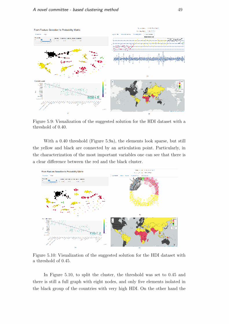
A novel committee - based clustering method 49
Figure 5.9: Visualization of the suggested solution for the HDI dataset with athreshold of 0.40.
With a 0.40 threshold (Figure 5.9a), the elements look sparse, but still
the yellow and black are connected by an articulation point. Particularly, in
the characterization of the most important variables one can see that there is
a clear difference between the red and the black cluster.
Figure 5.10: Visualization of the suggested solution for the HDI dataset witha threshold of 0.45.
In Figure 5.10, to split the cluster, the threshold was set to 0.45 and
there is still a full graph with eight nodes, and only five elements isolated in
the black group of the countries with very high HDI. On the other hand the
A novel committee - based clustering method 50
relationships between the red and yellow countries is less visible and there are
a lot more isolated countries from these categories.
5.3Discussion
In the comparison with individual clustering methods during the evaluation
of our method (in other words, using less computational resources), the Iris
and Wine datasets have the best results while Glass, Breast Cancer, Seeds
and Segmentation get similar results. The worst results were obtained with
the Yeast dataset.
Finally, the experiments reveal a detailed analysis of the datasets, but
aims at the relationships rather than the groups, allowing a more selective case
of study. They combine different points of view of the similarity matrix giving
a flexible tool to attack a wide range of problems. The use of the method and
the visual tools came in handy, highlighting key details that can solve or turn
the interest of a research and shed light beyond the clustering.
6Conclusion and Future Work
This work presented a new method based on ensemble clustering, which creates
a similarity matrix combining multiple partitions of the dataset using feature
selection and clustering methods. Finally, it joined all partitions in order to
obtain a consensus one that uses a transformation of the previously computed
similarity matrix as a distance matrix input in an other clustering process.
Also, it proposed a visual tool prototype that is capable to explore the dataset
from different points of view. This prototype shows to be a useful tool to deeply
analyze the connection between the elements, characterize the instances and
locate them on the map. This is an interesting approach for spatial analysis
where the number of elements is reduced. With all the results, the proposed
objectives had been accomplished in the research.
The experiments reveal a good performance of our method. They show
that it is better or similar when compared with the individual clustering
methods. Moreover, when it is compared with the ensemble clustering methods,
it also has better results.
For future research, some suggestions that may improve the quality of
our method are listed below:
– It would be interesting to study a voting mechanism to suggest the most
important variables, as well as to create a similarity matrix between the
variables to apply network analysis.
– There are several of metrics to measure the quality of the clusters, such
as the Davies-Buldin index, the Dunn’s index and the Calinsky-Harabasz
index. And would be interesting to see the quality of a clustering process
as a combination of these measures, giving the chance to enhance the
characteristics of the metrics, unbalance the results and customize the
method according to the scenario.
– The method is independent of the clustering method and feature selec-
tion algorithms, but it would be interesting to compare the results of
other methods, such as Diana and DBSCAN as well as other feature
selection techniques, such as Simulated Annealing or Principal Feature
Component.
A novel committee - based clustering method 52
– Sometimes the best solution, even when it has the best quality coefficient,
is not the expected or desired result. So it would be extremely useful to
set a ranking and return the top 10 recommended clusterings.
– To validate the visual tool, use the observational techniques and inter-
views.
Bibliography
[1] https://www.r-project.org/.
[2] http://www.isp.rj.gov.br/. Accessed: 20150315.
[3] http://www.ibge.gov.br/home/. Accessed: 20150425.
[4] http://www.upprj.com/. Accessed: 20151212.
[5] http://hdr.undp.org/en/data. Accessed: 20160715.
[6] Clustering. http://docplayer.net/
16145991-Clustering-dhs-10-6-10-7-10-9-10-10-10-4-3-10-4-4.
html. Accessed: 20150920.
[7] ALMEIDA, C.; FIOL GONZALEZ, S.; LOPES, H.; BARBOSA, S. ;
SOUZA, P. Analysis of the impact of upps deployment in rio de janeiro,
journal, 2016. submitted for publication.
[8] ARMANFARD, N.; REILLY, J. P. ; KOMEILI, M. IEEE transactions
on pattern analysis and machine intelligence. Local feature selection
for data classification, journal, v.38, n.6, p. 1217–1227, 2016.
[9] BOLON-CANEDO, V.; SANCHEZ-MARONO, N. ; ALONSO-
BETANZOS, A. Knowledge and information systems. A review of
feature selection methods on synthetic data, journal, v.34, n.3, p. 483–519,
2013.
[10] CAI, D.; ZHANG, C. ; HE, X. Unsupervised feature selection for
multi-cluster data. In: PROCEEDINGS OF THE 16TH ACM SIGKDD
INTERNATIONAL CONFERENCE ON KNOWLEDGE DISCOVERY AND
DATA MINING, p. 333–342. ACM, 2010.
[11] CHANDRASHEKAR, G.; SAHIN, F. Computers & Electrical Engin-
eering. A survey on feature selection methods, journal, v.40, n.1, p. 16–28,
2014.
[12] COVER, T. M.; THOMAS, J. A. Elements of information theory.
John Wiley & Sons, 2012.
A novel committee - based clustering method 54
[13] DASH, M.; LIU, H. Intelligent data analysis. Feature selection for
classification, journal, v.1, n.3, p. 131–156, 1997.
[14] DEMPSTER, A. P.; LAIRD, N. M. ; RUBIN, D. B. Journal of the royal
statistical society. Series B (methodological). Maximum likelihood
from incomplete data via the em algorithm, journal, p. 1–38, 1977.
[15] DHIR, C. S.; LEE, J. ; LEE, S.-Y. Knowledge and information
systems. Extraction of independent discriminant features for data with
asymmetric distribution, journal, v.30, n.2, p. 359–375, 2012.
[16] DIETTERICH, T. G. Ensemble methods in machine learning. In:
INTERNATIONAL WORKSHOP ON MULTIPLE CLASSIFIER SYSTEMS,
p. 1–15. Springer, 2000.
[17] DOAK, J. An evaluation of feature selection methods and their
application to computer security. University of California, Computer
Science, 1992.
[18] DY, J. G.; BRODLEY, C. E. Journal of machine learning research.
Feature selection for unsupervised learning, journal, v.5, n.Aug, p. 845–889,
2004.
[19] ESTER, M.; KRIEGEL, H.-P.; SANDER, J.; XU, X. ; OTHERS. A
density-based algorithm for discovering clusters in large spatial
databases with noise. In: KDD, volume 96, p. 226–231, 1996.
[20] EVERITT, B. Edward Arnold and Halsted Press,. Cluster analysis.
1993, journal, 1993.
[21] FARAHAT, A. K.; GHODSI, A. ; KAMEL, M. S. Knowledge and
information systems. Efficient greedy feature selection for unsupervised
learning, journal, v.35, n.2, p. 285–310, 2013.
[22] FERN, X. Z.; BRODLEY, C. E. Random projection for high
dimensional data clustering: A cluster ensemble approach. In:
ICML, volume 3, p. 186–193, 2003.
[23] FERN, X. Z.; BRODLEY, C. E. Solving cluster ensemble prob-
lems by bipartite graph partitioning. In: PROCEEDINGS OF
THE TWENTY-FIRST INTERNATIONAL CONFERENCE ON MACHINE
LEARNING, p. 36. ACM, 2004.
A novel committee - based clustering method 55
[24] FRED, A. L.; JAIN, A. K. IEEE transactions on pattern analysis
and machine intelligence. Combining multiple clusterings using evidence
accumulation, journal, v.27, n.6, p. 835–850, 2005.
[25] FUKUNAGA, K. Introduction to Statistical Pattern Recognition
(2Nd Ed.). San Diego, CA, USA: Academic Press Professional, Inc., 1990.
[26] GAN, G.; MA, C. ; WU, J. Data clustering: theory, algorithms, and
applications, volume 20. Siam, 2007.
[27] GUYON, I.; ELISSEEFF, A. Journal of machine learning research.
An introduction to variable and feature selection, journal, v.3, n.Mar, p. 1157–
1182, 2003.
[28] GUYON, I.; ELISSEEFF, A. An introduction to feature extraction.
In: FEATURE EXTRACTION, p. 1–25. Springer, 2006.
[29] HOLTEN, D. IEEE Transactions on visualization and computer
graphics. Hierarchical edge bundles: Visualization of adjacency relations in
hierarchical data, journal, v.12, n.5, p. 741–748, 2006.
[30] HUANG, D.; LAI, J.-H. ; WANG, C.-D. Neurocomputing. Combining
multiple clusterings via crowd agreement estimation and multi-granularity link
analysis, journal, v.170, p. 240–250, 2015.
[31] IAM-ON, N.; BOONGOEN, T. ; GARRETT, S. Refining pairwise
similarity matrix for cluster ensemble problem with cluster re-
lations. In: INTERNATIONAL CONFERENCE ON DISCOVERY SCIENCE,
p. 222–233. Springer, 2008.
[32] IAM-ON, N.; BOONGOEN, T.; GARRETT, S. ; PRICE, C. IEEE
transactions on pattern analysis and machine intelligence. A
link-based approach to the cluster ensemble problem, journal, v.33, n.12, p.
2396–2409, 2011.
[33] JOLLIFFE, I. Principal component analysis. Wiley Online Library,
2002.
[34] JOVIC, A.; BRKIC, K. ; BOGUNOVIC, N. A review of feature selec-
tion methods with applications. In: INFORMATION AND COMMU-
NICATION TECHNOLOGY, ELECTRONICS AND MICROELECTRONICS
(MIPRO), 2015 38TH INTERNATIONAL CONVENTION ON, p. 1200–1205.
IEEE, 2015.
A novel committee - based clustering method 56
[35] KAUFMAN, L.; ROUSSEEUW, P. J. Finding groups in data: an
introduction to cluster analysis. John Wiley & Sons, 1990.
[36] KOHAVI, R.; JOHN, G. H. Artificial intelligence. Wrappers for feature
subset selection, journal, v.97, n.1, p. 273–324, 1997.
[37] KOLACZYK, E. D.; CSARDI, G. Statistical analysis of network
data with R. Springer, 2014.
[38] LI, N.; LATECKI, L. J. Clustering aggregation as maximum-
weight independent set. In: ADVANCES IN NEURAL INFORMATION
PROCESSING SYSTEMS, p. 782–790, 2012.
[39] LI, T.; DING, C. Mij. Weighted consensus clustering, journal, v.1, n.2,
2008.
[40] LICHMAN, M. UCI machine learning repository, 2013.
[41] LIU, H.; MOTODA, H. Computational methods of feature selec-
tion. CRC Press, 2007.
[42] LU, Y.; COHEN, I.; ZHOU, X. S. ; TIAN, Q. Feature selection using
principal feature analysis. In: PROCEEDINGS OF THE 15TH ACM
INTERNATIONAL CONFERENCE ON MULTIMEDIA, p. 301–304. ACM,
2007.
[43] MACQUEEN, J. Some methods for classification and analysis of
multivariate observations. In: PROCEEDINGS OF THE FIFTH BERKE-
LEY SYMPOSIUM ON MATHEMATICAL STATISTICS AND PROBABIL-
ITY, VOLUME 1: STATISTICS, p. 281–297, Berkeley, Calif., 1967. University
of California Press.
[44] MELNYKOV, V.; CHEN, W.-C. ; MAITRA, R. Journal of Statistical
Software. Mixsim: An r package for simulating data to study performance
of clustering algorithms, journal, v.51, n.12, p. 1–25, 2012.
[45] MENDES-MOREIRA, J.; SOARES, C.; JORGE, A. M. ; SOUSA, J.
F. D. ACM Computing Surveys (CSUR). Ensemble approaches for
regression: A survey, journal, v.45, n.1, p. 10, 2012.
[46] MIMAROGLU, S.; AKSEHIRLI, E. IEEE/ACM Transactions on
Computational Biology and Bioinformatics (TCBB). Diclens:
Divisive clustering ensemble with automatic cluster number, journal, v.9, n.2,
p. 408–420, 2012.
A novel committee - based clustering method 57
[47] MURTY, M. N.; DEVI, V. S. Pattern recognition: An algorithmic
approach. Springer Science & Business Media, 2011.
[48] NG, R. T.; HAN, J. IEEE transactions on knowledge and data
engineering. Clarans: A method for clustering objects for spatial data
mining, journal, v.14, n.5, p. 1003–1016, 2002.
[49] PARK, H.-S.; JUN, C.-H. Expert Systems with Applications. A
simple and fast algorithm for k-medoids clustering, journal, v.36, n.2, p. 3336–
3341, 2009.
[50] PETER, T. J.; SOMASUNDARAM, K. International Journal of
Scientific and Research Publications. Study and development of novel
feature selection framework for heart disease prediction, journal, v.2, n.10, p.
1–7, 2012.
[51] ROUSSEEUW, P. J. Journal of computational and applied math-
ematics. Silhouettes: a graphical aid to the interpretation and validation of
cluster analysis, journal, v.20, p. 53–65, 1987.
[52] STEINBACH, M.; ERTOZ, L. ; KUMAR, V. The challenges of clus-
tering high dimensional data. In: NEW DIRECTIONS IN STATISTICAL
PHYSICS, p. 273–309. Springer, 2004.
[53] STREHL, A.; GHOSH, J. Journal of machine learning research.
Cluster ensembles—a knowledge reuse framework for combining multiple
partitions, journal, v.3, n.Dec, p. 583–617, 2002.
[54] TOPCHY, A.; JAIN, A. K. ; PUNCH, W. Combining multiple
weak clusterings. In: DATA MINING, 2003. ICDM 2003. THIRD IEEE
INTERNATIONAL CONFERENCE ON, p. 331–338. IEEE, 2003.
[55] TOPCHY, A. P.; JAIN, A. K. ; PUNCH, W. F. A mixture model for
clustering ensembles. In: SDM, p. 379–390. SIAM, 2004.
[56] VEGA-PONS, S.; RUIZ-SHULCLOPER, J. International Journal
of Pattern Recognition and Artificial Intelligence. A survey of
clustering ensemble algorithms, journal, v.25, n.03, p. 337–372, 2011.
[57] VELMURUGAN, T.; SANTHANAM, T. Journal of computer sci-
ence. Computational complexity between k-means and k-medoids clustering
algorithms for normal and uniform distributions of data points, journal, v.6,
n.3, p. 363, 2010.
A novel committee - based clustering method 58
[58] WANG, X.; YANG, C. ; ZHOU, J. Pattern Recognition. Clustering
aggregation by probability accumulation, journal, v.42, n.5, p. 668–675, 2009.
[59] WILKINSON, L.; FRIENDLY, M. The American Statistician. The
history of the cluster heat map, journal, 2012.
[60] XU, D.; TIAN, Y. Annals of Data Science. A comprehensive survey of
clustering algorithms, journal, v.2, n.2, p. 165–193, 2015.
[61] YI, J.; YANG, T.; JIN, R.; JAIN, A. K. ; MAHDAVI, M. Robust
ensemble clustering by matrix completion. In: 2012 IEEE 12TH
INTERNATIONAL CONFERENCE ON DATA MINING, p. 1176–1181. IEEE,
2012.
[62] ZHANG, C.; MA, Y. Ensemble machine learning. Springer, 2012.
[63] ZHAO, Z.; LIU, H. Spectral feature selection for supervised and
unsupervised learning. In: PROCEEDINGS OF THE 24TH INTERNA-
TIONAL CONFERENCE ON MACHINE LEARNING, p. 1151–1157. ACM,
2007.
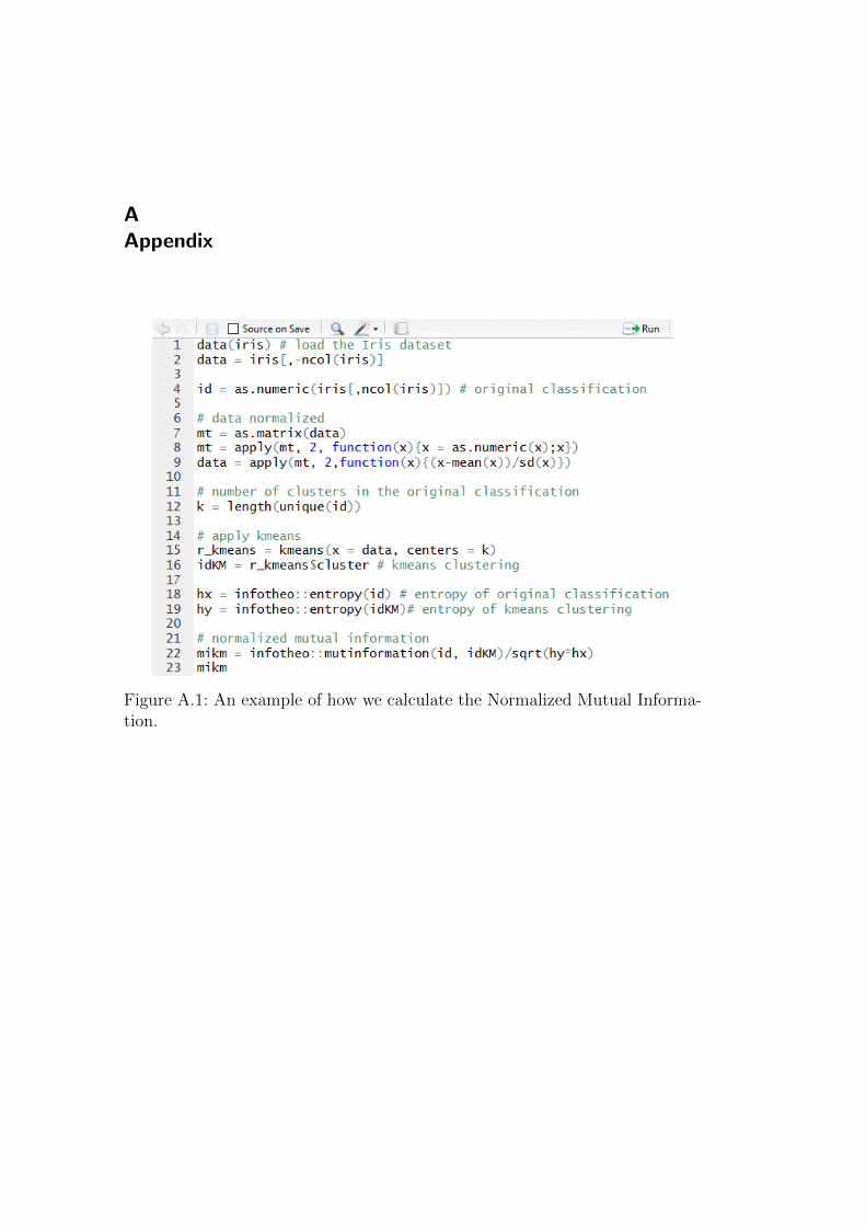
AAppendix
Figure A.1: An example of how we calculate the Normalized Mutual Informa-tion.

BAppendix
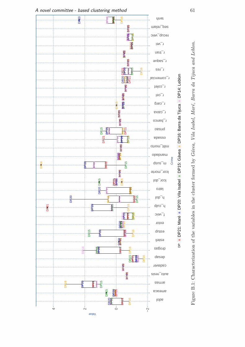
A novel committee - based clustering method 61
●
●
●
● ●
●
●
●
DP
21
DP
21
DP
21
DP
21D
P21
DP
21
DP
21
DP
21
DP
21D
P21
DP
21
DP
21
DP
21
DP
21D
P21
DP
21
DP
21D
P21
DP
21
DP
21D
P21
DP
21
DP
21
DP
21D
P21
DP
21
DP
21D
P21
DP
21
DP
21D
P21
DP
21
DP
21
DP
21
DP
20
DP
20
DP
20
DP
20
DP
20
DP
20
DP
20
DP
20
DP
20
DP
20D
P20
DP
20
DP
20
DP
20D
P20
DP
20
DP
20D
P20
DP
20
DP
20D
P20
DP
20
DP
20
DP
20
DP
20
DP
20
DP
20D
P20
DP
20
DP
20
DP
20
DP
20
DP
20
DP
20
DP
15
DP
15
DP
15
DP
15
DP
15
DP
15
DP
15
DP
15D
P15
DP
15D
P15
DP
15D
P15
DP
15D
P15
DP
15
DP
15D
P15
DP
15
DP
15
DP
15
DP
15
DP
15
DP
15
DP
15
DP
15D
P15
DP
15
DP
15
DP
15
DP
15
DP
15D
P15
DP
15
DP
16
DP
16
DP
16
DP
16D
P16
DP
16
DP
16
DP
16
DP
16
DP
16D
P16
DP
16
DP
16
DP
16
DP
16D
P16
DP
16D
P16
DP
16
DP
16
DP
16
DP
16
DP
16
DP
16
DP
16
DP
16
DP
16
DP
16D
P16
DP
16
DP
16
DP
16
DP
16
DP
16D
P14
DP
14
DP
14D
P14
DP
14
DP
14
DP
14
DP
14
DP
14
DP
14
DP
14D
P14
DP
14
DP
14D
P14
DP
14
DP
14D
P14
DP
14
DP
14
DP
14D
P14
DP
14
DP
14
DP
14
DP
14
DP
14D
P14
DP
14
DP
14D
P14
DP
14
DP
14
DP
14
−2024
adol
ameaca
armas
auto_resis
cadaver
desap
drogas
esteli
estup
extor
f_veic
h_culp
h_dol
latro
lcor_dol
lcor_morte
m_susp
mandado
milit_morto
ossada
prisao
r_banco
r_caixa
r_carg
r_cel
r_colet
r_comercial
r_res
r_saque
r_tran
r_vei
recup_veic
seq_relam
tenh
Crim
e
Value
DP
aa
aa
aD
P21
: Mar
éD
P20
: Vila
Isab
elD
P15
: Gáv
eaD
P16
: Bar
ra d
a T
ijuca
DP
14: L
eblo
n
Fig
ure
B.1
:C
har
acte
riza
tion
ofth
eva
riab
les
inth
ecl
ust
erfo
rmed
by
Gav
ea,
Vil
aIs
abel
,M
are,
Bar
rada
Tij
uca
and
Leb
lon
.
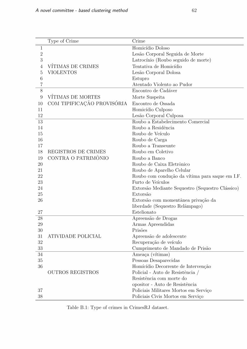
A novel committee - based clustering method 62
Type of Crime Crime
1 Homicıdio Doloso2 Lesao Corporal Seguida de Morte3 Latrocınio (Roubo seguido de morte)
4 VITIMAS DE CRIMES Tentativa de Homicıdio5 VIOLENTOS Lesao Corporal Dolosa6 Estupro7 Atentado Violento ao Pudor8 Encontro de Cadaver
9 VITIMAS DE MORTES Morte Suspeita
10 COM TIPIFICACAO PROVISORIA Encontro de Ossada11 Homicıdio Culposo12 Lesao Corporal Culposa13 Roubo a Estabelecimento Comercial14 Roubo a Residencia15 Roubo de Veıculo16 Roubo de Carga17 Roubo a Transeunte18 REGISTROS DE CRIMES Roubo em Coletivo
19 CONTRA O PATRIMONIO Roubo a Banco20 Roubo de Caixa Eletronico21 Roubo de Aparelho Celular22 Roubo com conducao da vıtima para saque em I.F.23 Furto de Veıculos24 Extorsao Mediante Sequestro (Sequestro Classico)25 Extorsao26 Extorsao com momentanea privacao da
liberdade (Sequestro Relampago)27 Estelionato28 Apreensao de Drogas29 Armas Apreendidas30 Prisoes31 ATIVIDADE POLICIAL Apreensao de adolescente32 Recuperacao de veıculo33 Cumprimento de Mandado de Prisao34 Ameaca (vıtimas)35 Pessoas Desaparecidas36 Homıcıdio Decorrente de Intervencao
OUTROS REGISTROS Policial - Auto de Resistencia /Resistencia com morte doopositor - Auto de Resistencia
37 Policiais Militares Mortos em Servico38 Policiais Civis Mortos em Servico
Table B.1: Type of crimes in CrimesRJ dataset.
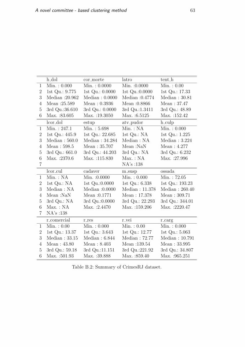
A novel committee - based clustering method 63
h dol cor morte latro tent h1 Min. : 0.000 Min. : 0.0000 Min. :0.0000 Min. : 0.002 1st Qu.: 9.775 1st Qu.: 0.0000 1st Qu.:0.0000 1st Qu.: 17.333 Median :20.962 Median : 0.0000 Median :0.4774 Median : 30.814 Mean :25.589 Mean : 0.3936 Mean :0.8866 Mean : 37.475 3rd Qu.:36.610 3rd Qu.: 0.0000 3rd Qu.:1.3411 3rd Qu.: 48.896 Max. :83.605 Max. :19.3050 Max. :6.5125 Max. :152.42
lcor dol estup atv pudor h culp1 Min. : 247.1 Min. : 5.698 Min. : NA Min. : 0.0002 1st Qu.: 445.9 1st Qu.: 22.685 1st Qu.: NA 1st Qu.: 1.2253 Median : 560.0 Median : 34.284 Median : NA Median : 3.2244 Mean : 598.5 Mean : 35.707 Mean :NaN Mean : 4.2775 3rd Qu.: 661.0 3rd Qu.: 44.203 3rd Qu.: NA 3rd Qu.: 6.2326 Max. :2370.6 Max. :115.830 Max. : NA Max. :27.9967 NA’s :138
lcor cul cadaver m susp ossada1 Min. : NA Min. :0.0000 Min. : 0.000 Min. : 72.052 1st Qu.: NA 1st Qu.:0.0000 1st Qu.: 6.338 1st Qu.: 193.233 Median : NA Median :0.0000 Median : 11.378 Median : 260.404 Mean :NaN Mean :0.1771 Mean : 17.378 Mean : 309.715 3rd Qu.: NA 3rd Qu.:0.0000 3rd Qu.: 22.293 3rd Qu.: 344.016 Max. : NA Max. :2.4470 Max. :159.206 Max. :2220.477 NA’s :138
r comercial r res r vei r carg1 Min. : 0.00 Min. : 0.000 Min. : 0.00 Min. : 0.0002 1st Qu.: 13.37 1st Qu.: 3.643 1st Qu.: 12.77 1st Qu.: 5.0633 Median : 33.15 Median : 6.844 Median : 72.77 Median : 10.7914 Mean : 43.80 Mean : 8.403 Mean :139.54 Mean : 33.9955 3rd Qu.: 59.18 3rd Qu.:11.151 3rd Qu.:221.92 3rd Qu.: 34.8076 Max. :501.93 Max. :39.888 Max. :859.40 Max. :965.251
Table B.2: Summary of CrimesRJ dataset.
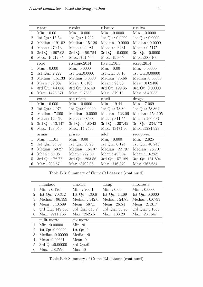
A novel committee - based clustering method 64
r tran r colet r banco r caixa1 Min. : 0.00 Min. : 0.000 Min. : 0.0000 Min. : 0.00002 1st Qu.: 15.54 1st Qu.: 1.202 1st Qu.: 0.0000 1st Qu.: 0.00003 Median : 191.02 Median : 15.126 Median : 0.0000 Median : 0.00004 Mean : 470.13 Mean : 44.081 Mean : 0.3231 Mean : 0.51755 3rd Qu.: 597.03 3rd Qu.: 50.754 3rd Qu.: 0.0000 3rd Qu.: 0.00006 Max. :10212.35 Max. :791.506 Max. :19.3050 Max. :38.6100
r cel r saque 2014 f veic 2014 e seq 20141 Min. : 0.000 Min. :0.0000 Min. : 0.00 Min. :0.000002 1st Qu.: 2.222 1st Qu.:0.0000 1st Qu.: 50.10 1st Qu.:0.000003 Median : 15.133 Median :0.0000 Median : 75.66 Median :0.000004 Mean : 52.887 Mean :0.5183 Mean : 98.58 Mean :0.024865 3rd Qu.: 54.058 3rd Qu.:0.6140 3rd Qu.:129.36 3rd Qu.:0.000006 Max. :1428.571 Max. :9.7688 Max. :579.15 Max. :3.43053
extor seq relam esteli drogas1 Min. : 0.000 Min. : 0.0000 Min. : 19.44 Min. : 7.0692 1st Qu.: 4.976 1st Qu.: 0.0000 1st Qu.: 78.80 1st Qu.: 78.8643 Median : 7.800 Median : 0.0000 Median : 123.06 Median : 154.1054 Mean : 12.463 Mean : 0.8638 Mean : 311.55 Mean : 266.6375 3rd Qu.: 13.147 3rd Qu.: 1.0842 3rd Qu.: 207.45 3rd Qu.: 234.1736 Max. :193.050 Max. :14.2596 Max. :13474.90 Max. :5284.923
armas prisao adol recup veic1 Min. : 11.01 Min. : 0.00 Min. : 0.000 Min. : 2.8252 1st Qu.: 34.32 1st Qu.: 80.93 1st Qu.: 6.124 1st Qu.: 40.7433 Median : 50.27 Median : 154.07 Median : 22.797 Median : 75.7074 Mean : 60.08 Mean : 227.69 Mean : 49.004 Mean :116.2525 3rd Qu.: 72.77 3rd Qu.: 283.58 3rd Qu.: 57.189 3rd Qu.:161.8046 Max. :209.57 Max. :3702.38 Max. :716.379 Max. :767.654
Table B.3: Summary of CrimesRJ dataset (continued).
mandado ameaca desap auto resis1 Min. : 6.126 Min. : 266.1 Min. : 0.00 Min. : 0.00002 1st Qu.: 70.312 1st Qu.: 430.6 1st Qu.: 14.09 1st Qu.: 0.00003 Median : 96.399 Median : 542.0 Median : 24.85 Median : 0.67934 Mean : 140.589 Mean : 587.1 Mean : 26.54 Mean : 2.43175 3rd Qu.: 149.686 3rd Qu.: 648.2 3rd Qu.: 33.96 3rd Qu.: 3.10656 Max. :2211.166 Max. :2625.5 Max. :133.29 Max. :23.7647
milit morto civ morto1 Min. :0.00000 Min. :02 1st Qu.:0.00000 1st Qu.:03 Median :0.00000 Median :04 Mean :0.09661 Mean :05 3rd Qu.:0.00000 3rd Qu.:06 Max. :2.82554 Max. :0
Table B.4: Summary of CrimesRJ dataset (continued).
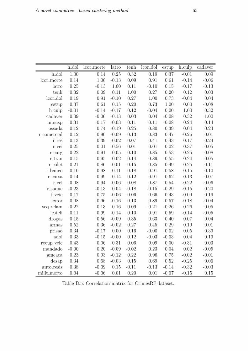
A novel committee - based clustering method 65
h dol lcor morte latro tenh lcor dol estup h culp cadaver
h dol 1.00 0.14 0.25 0.32 0.19 0.37 -0.01 0.09lcor morte 0.14 1.00 -0.13 0.09 0.91 0.61 -0.14 -0.06
latro 0.25 -0.13 1.00 0.11 -0.10 0.15 -0.17 -0.13tenh 0.32 0.09 0.11 1.00 0.27 0.20 0.12 0.03
lcor dol 0.19 0.91 -0.10 0.27 1.00 0.73 -0.04 0.04estup 0.37 0.61 0.15 0.20 0.73 1.00 0.00 -0.08
h culp -0.01 -0.14 -0.17 0.12 -0.04 0.00 1.00 0.32cadaver 0.09 -0.06 -0.13 0.03 0.04 -0.08 0.32 1.00m susp 0.31 -0.17 -0.03 0.11 -0.11 -0.08 0.24 0.14ossada 0.12 0.74 -0.19 0.25 0.80 0.39 0.04 0.24
r comercial 0.12 0.90 -0.09 0.13 0.83 0.47 -0.26 0.01r res 0.13 0.39 -0.02 0.07 0.41 0.43 0.17 0.24r vei 0.25 -0.01 0.56 -0.01 0.01 0.02 -0.37 -0.05
r carg 0.22 0.91 -0.05 0.10 0.85 0.53 -0.25 -0.08r tran 0.15 0.95 -0.02 0.14 0.89 0.55 -0.24 -0.05r colet 0.21 0.86 0.01 0.15 0.85 0.49 -0.25 0.11
r banco 0.10 0.98 -0.11 0.18 0.91 0.58 -0.15 -0.10r caixa 0.14 0.99 -0.14 0.12 0.91 0.62 -0.13 -0.07
r cel 0.08 0.94 -0.06 0.08 0.87 0.54 -0.22 -0.06r saque -0.23 -0.13 0.04 -0.18 -0.15 -0.29 -0.15 0.20
f veic 0.17 0.75 -0.06 0.06 0.66 0.43 -0.09 0.19extor 0.08 0.96 -0.16 0.13 0.89 0.57 -0.18 -0.04
seq relam -0.22 -0.13 0.16 -0.09 -0.21 -0.26 -0.26 -0.05esteli 0.11 0.99 -0.14 0.10 0.91 0.59 -0.14 -0.05
drogas 0.15 0.56 -0.09 0.35 0.63 0.40 0.07 0.04armas 0.52 0.36 -0.02 0.27 0.45 0.29 0.19 0.01prisao 0.34 -0.17 0.00 0.16 -0.00 0.02 0.05 0.39
adol 0.33 -0.15 -0.00 0.12 -0.03 -0.03 0.04 0.19recup veic 0.43 0.06 0.31 0.06 0.09 0.00 -0.31 0.03mandado -0.00 0.20 -0.09 -0.02 0.23 0.04 0.02 -0.05
ameaca 0.23 0.93 -0.12 0.22 0.96 0.75 -0.02 -0.01desap 0.34 0.68 -0.03 0.15 0.69 0.52 -0.25 0.06
auto resis 0.38 -0.09 0.15 -0.11 -0.13 -0.14 -0.32 -0.03milit morto 0.04 -0.06 0.01 0.20 0.01 -0.07 -0.15 0.15
Table B.5: Correlation matrix for CrimesRJ dataset.
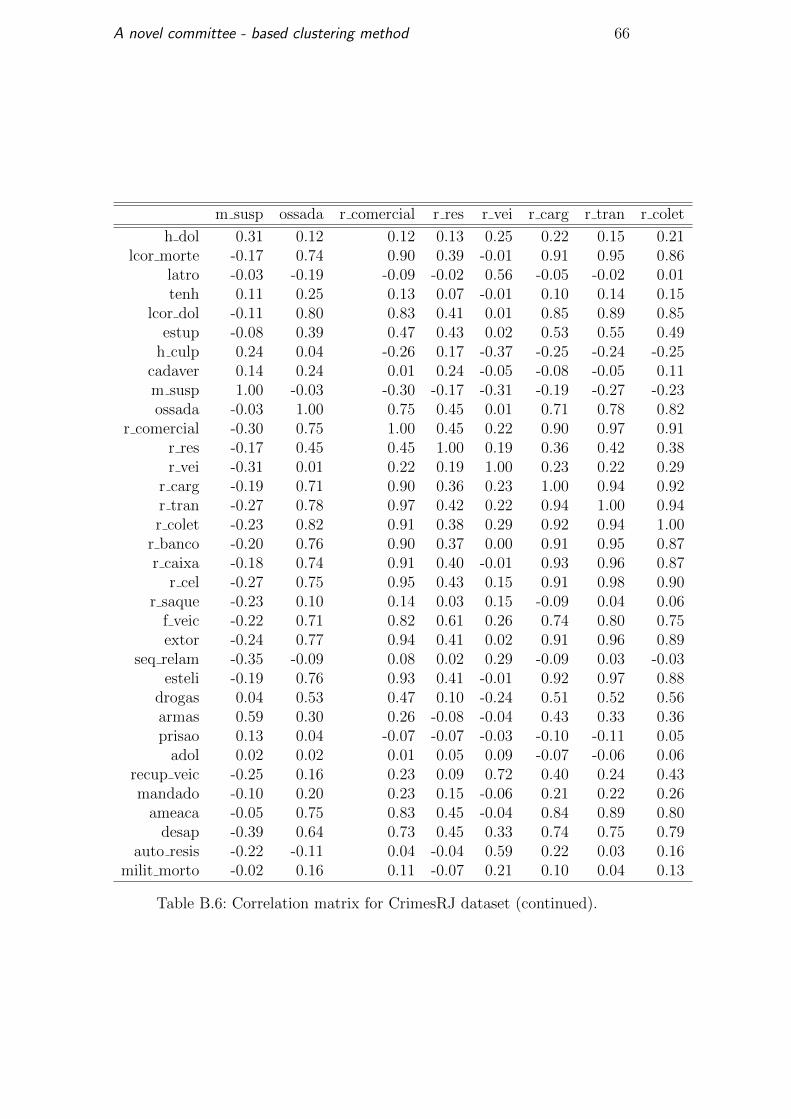
A novel committee - based clustering method 66
m susp ossada r comercial r res r vei r carg r tran r colet
h dol 0.31 0.12 0.12 0.13 0.25 0.22 0.15 0.21lcor morte -0.17 0.74 0.90 0.39 -0.01 0.91 0.95 0.86
latro -0.03 -0.19 -0.09 -0.02 0.56 -0.05 -0.02 0.01tenh 0.11 0.25 0.13 0.07 -0.01 0.10 0.14 0.15
lcor dol -0.11 0.80 0.83 0.41 0.01 0.85 0.89 0.85estup -0.08 0.39 0.47 0.43 0.02 0.53 0.55 0.49
h culp 0.24 0.04 -0.26 0.17 -0.37 -0.25 -0.24 -0.25cadaver 0.14 0.24 0.01 0.24 -0.05 -0.08 -0.05 0.11m susp 1.00 -0.03 -0.30 -0.17 -0.31 -0.19 -0.27 -0.23ossada -0.03 1.00 0.75 0.45 0.01 0.71 0.78 0.82
r comercial -0.30 0.75 1.00 0.45 0.22 0.90 0.97 0.91r res -0.17 0.45 0.45 1.00 0.19 0.36 0.42 0.38r vei -0.31 0.01 0.22 0.19 1.00 0.23 0.22 0.29
r carg -0.19 0.71 0.90 0.36 0.23 1.00 0.94 0.92r tran -0.27 0.78 0.97 0.42 0.22 0.94 1.00 0.94r colet -0.23 0.82 0.91 0.38 0.29 0.92 0.94 1.00
r banco -0.20 0.76 0.90 0.37 0.00 0.91 0.95 0.87r caixa -0.18 0.74 0.91 0.40 -0.01 0.93 0.96 0.87
r cel -0.27 0.75 0.95 0.43 0.15 0.91 0.98 0.90r saque -0.23 0.10 0.14 0.03 0.15 -0.09 0.04 0.06
f veic -0.22 0.71 0.82 0.61 0.26 0.74 0.80 0.75extor -0.24 0.77 0.94 0.41 0.02 0.91 0.96 0.89
seq relam -0.35 -0.09 0.08 0.02 0.29 -0.09 0.03 -0.03esteli -0.19 0.76 0.93 0.41 -0.01 0.92 0.97 0.88
drogas 0.04 0.53 0.47 0.10 -0.24 0.51 0.52 0.56armas 0.59 0.30 0.26 -0.08 -0.04 0.43 0.33 0.36prisao 0.13 0.04 -0.07 -0.07 -0.03 -0.10 -0.11 0.05
adol 0.02 0.02 0.01 0.05 0.09 -0.07 -0.06 0.06recup veic -0.25 0.16 0.23 0.09 0.72 0.40 0.24 0.43mandado -0.10 0.20 0.23 0.15 -0.06 0.21 0.22 0.26
ameaca -0.05 0.75 0.83 0.45 -0.04 0.84 0.89 0.80desap -0.39 0.64 0.73 0.45 0.33 0.74 0.75 0.79
auto resis -0.22 -0.11 0.04 -0.04 0.59 0.22 0.03 0.16milit morto -0.02 0.16 0.11 -0.07 0.21 0.10 0.04 0.13
Table B.6: Correlation matrix for CrimesRJ dataset (continued).
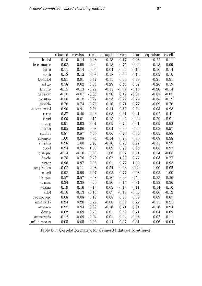
A novel committee - based clustering method 67
r banco r caixa r cel r saque f veic extor seq relam estelih dol 0.10 0.14 0.08 -0.23 0.17 0.08 -0.22 0.11
lcor morte 0.98 0.99 0.94 -0.13 0.75 0.96 -0.13 0.99latro -0.11 -0.14 -0.06 0.04 -0.06 -0.16 0.16 -0.14tenh 0.18 0.12 0.08 -0.18 0.06 0.13 -0.09 0.10
lcor dol 0.91 0.91 0.87 -0.15 0.66 0.89 -0.21 0.91estup 0.58 0.62 0.54 -0.29 0.43 0.57 -0.26 0.59
h culp -0.15 -0.13 -0.22 -0.15 -0.09 -0.18 -0.26 -0.14cadaver -0.10 -0.07 -0.06 0.20 0.19 -0.04 -0.05 -0.05m susp -0.20 -0.18 -0.27 -0.23 -0.22 -0.24 -0.35 -0.19ossada 0.76 0.74 0.75 0.10 0.71 0.77 -0.09 0.76
r comercial 0.90 0.91 0.95 0.14 0.82 0.94 0.08 0.93r res 0.37 0.40 0.43 0.03 0.61 0.41 0.02 0.41r vei 0.00 -0.01 0.15 0.15 0.26 0.02 0.29 -0.01
r carg 0.91 0.93 0.91 -0.09 0.74 0.91 -0.09 0.92r tran 0.95 0.96 0.98 0.04 0.80 0.96 0.03 0.97r colet 0.87 0.87 0.90 0.06 0.75 0.89 -0.03 0.88
r banco 1.00 0.98 0.94 -0.14 0.75 0.96 -0.08 0.98r caixa 0.98 1.00 0.95 -0.10 0.76 0.97 -0.11 0.99
r cel 0.94 0.95 1.00 0.09 0.79 0.96 0.08 0.97r saque -0.14 -0.10 0.09 1.00 0.07 0.01 0.54 -0.05
f veic 0.75 0.76 0.79 0.07 1.00 0.77 0.03 0.77extor 0.96 0.97 0.96 0.01 0.77 1.00 0.04 0.98
seq relam -0.08 -0.11 0.08 0.54 0.03 0.04 1.00 -0.05esteli 0.98 0.99 0.97 -0.05 0.77 0.98 -0.05 1.00
drogas 0.57 0.57 0.48 -0.20 0.30 0.54 -0.33 0.56armas 0.34 0.38 0.29 -0.30 0.15 0.31 -0.32 0.36prisao -0.19 -0.16 -0.18 0.09 -0.15 -0.11 -0.14 -0.16
adol -0.16 -0.13 -0.13 0.07 -0.10 -0.06 -0.06 -0.12recup veic 0.08 0.08 0.15 0.08 0.20 0.09 0.09 0.07mandado 0.24 0.20 0.22 -0.06 0.04 0.22 -0.11 0.21
ameaca 0.92 0.94 0.89 -0.16 0.71 0.91 -0.16 0.94desap 0.68 0.69 0.70 0.01 0.62 0.71 -0.04 0.69
auto resis -0.12 -0.09 -0.04 0.01 0.04 -0.08 0.07 -0.11milit morto -0.05 -0.05 -0.03 0.14 0.07 -0.01 -0.06 -0.04
Table B.7: Correlation matrix for CrimesRJ dataset (continued).
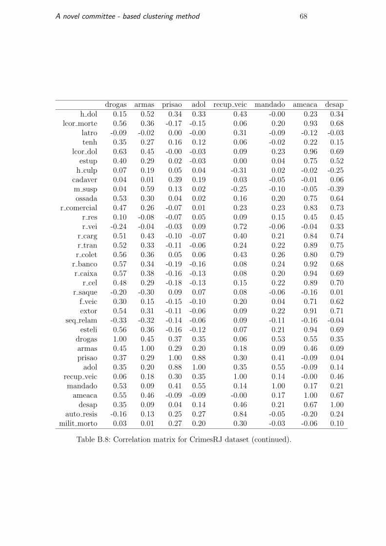
A novel committee - based clustering method 68
drogas armas prisao adol recup veic mandado ameaca desaph dol 0.15 0.52 0.34 0.33 0.43 -0.00 0.23 0.34
lcor morte 0.56 0.36 -0.17 -0.15 0.06 0.20 0.93 0.68latro -0.09 -0.02 0.00 -0.00 0.31 -0.09 -0.12 -0.03tenh 0.35 0.27 0.16 0.12 0.06 -0.02 0.22 0.15
lcor dol 0.63 0.45 -0.00 -0.03 0.09 0.23 0.96 0.69estup 0.40 0.29 0.02 -0.03 0.00 0.04 0.75 0.52
h culp 0.07 0.19 0.05 0.04 -0.31 0.02 -0.02 -0.25cadaver 0.04 0.01 0.39 0.19 0.03 -0.05 -0.01 0.06m susp 0.04 0.59 0.13 0.02 -0.25 -0.10 -0.05 -0.39ossada 0.53 0.30 0.04 0.02 0.16 0.20 0.75 0.64
r comercial 0.47 0.26 -0.07 0.01 0.23 0.23 0.83 0.73r res 0.10 -0.08 -0.07 0.05 0.09 0.15 0.45 0.45r vei -0.24 -0.04 -0.03 0.09 0.72 -0.06 -0.04 0.33
r carg 0.51 0.43 -0.10 -0.07 0.40 0.21 0.84 0.74r tran 0.52 0.33 -0.11 -0.06 0.24 0.22 0.89 0.75r colet 0.56 0.36 0.05 0.06 0.43 0.26 0.80 0.79
r banco 0.57 0.34 -0.19 -0.16 0.08 0.24 0.92 0.68r caixa 0.57 0.38 -0.16 -0.13 0.08 0.20 0.94 0.69
r cel 0.48 0.29 -0.18 -0.13 0.15 0.22 0.89 0.70r saque -0.20 -0.30 0.09 0.07 0.08 -0.06 -0.16 0.01
f veic 0.30 0.15 -0.15 -0.10 0.20 0.04 0.71 0.62extor 0.54 0.31 -0.11 -0.06 0.09 0.22 0.91 0.71
seq relam -0.33 -0.32 -0.14 -0.06 0.09 -0.11 -0.16 -0.04esteli 0.56 0.36 -0.16 -0.12 0.07 0.21 0.94 0.69
drogas 1.00 0.45 0.37 0.35 0.06 0.53 0.55 0.35armas 0.45 1.00 0.29 0.20 0.18 0.09 0.46 0.09prisao 0.37 0.29 1.00 0.88 0.30 0.41 -0.09 0.04
adol 0.35 0.20 0.88 1.00 0.35 0.55 -0.09 0.14recup veic 0.06 0.18 0.30 0.35 1.00 0.14 -0.00 0.46mandado 0.53 0.09 0.41 0.55 0.14 1.00 0.17 0.21
ameaca 0.55 0.46 -0.09 -0.09 -0.00 0.17 1.00 0.67desap 0.35 0.09 0.04 0.14 0.46 0.21 0.67 1.00
auto resis -0.16 0.13 0.25 0.27 0.84 -0.05 -0.20 0.24milit morto 0.03 0.01 0.27 0.20 0.30 -0.03 -0.06 0.10
Table B.8: Correlation matrix for CrimesRJ dataset (continued).
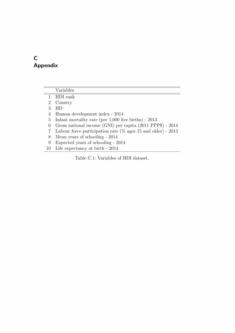
CAppendix
Variables
1 HDI rank2 Country3 HD4 Human development index - 20145 Infant mortality rate (per 1,000 live births) - 20136 Gross national income (GNI) per capita (2011 PPP$) - 20147 Labour force participation rate (% ages 15 and older) - 20138 Mean years of schooling - 20149 Expected years of schooling - 2014
10 Life expectancy at birth - 2014
Table C.1: Variables of HDI dataset.
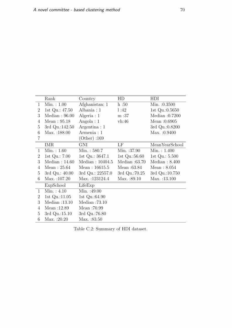
A novel committee - based clustering method 70
Rank Country HD HDI1 Min. : 1.00 Afghanistan: 1 h :50 Min. :0.35002 1st Qu.: 47.50 Albania : 1 l :42 1st Qu.:0.56503 Median : 96.00 Algeria : 1 m :37 Median :0.72004 Mean : 95.18 Angola : 1 vh:46 Mean :0.69055 3rd Qu.:142.50 Argentina : 1 3rd Qu.:0.82006 Max. :188.00 Armenia : 1 Max. :0.94007 (Other) :169
IMR GNI LF MeanYearSchool1 Min. : 1.60 Min. : 580.7 Min. :37.90 Min. : 1.4002 1st Qu.: 7.00 1st Qu.: 3647.1 1st Qu.:56.60 1st Qu.: 5.5003 Median : 14.60 Median : 10404.5 Median :63.70 Median : 8.4004 Mean : 25.64 Mean : 16615.5 Mean :63.84 Mean : 8.0545 3rd Qu.: 40.00 3rd Qu.: 22557.0 3rd Qu.:70.25 3rd Qu.:10.7506 Max. :107.20 Max. :123124.4 Max. :89.10 Max. :13.100
ExpSchool LifeExp1 Min. : 4.10 Min. :49.002 1st Qu.:11.05 1st Qu.:64.903 Median :13.10 Median :73.104 Mean :12.89 Mean :70.995 3rd Qu.:15.10 3rd Qu.:76.806 Max. :20.20 Max. :83.50
Table C.2: Summary of HDI dataset.