Some Techniques for Solving Recurrences - ict.ac.cnbioinfo.ict.ac.cn/~dbu/AlgorithmCourses/Lectures/Lec5-solving... · Some Techniques for Solving Recurrences ... CR Categorws" 5.25,

Some Techniques for Solving Recurrences

GEORGE S. LUEKER

Department of Information and Computer Scwnce, Unwers~ty of California, lrvine, California 92717

Some techmques for solving recurrences are presented, along with examples of how these recurrences arise in the analysis of algorithms. In addition, probability generating functions are discussed and used to analyze problems in computer science.

Keywords and Phrases: recurrences, characteristic equations, generating functions, probability generating functions, analysis of algorithms, asymptotic analysis

CR Categorws" 5.25, 5.30, 5.5

INTRODUCTION

The analysis of a problem in computer science often involves a sequence of numbers. For example, when determining the amount of time used by an algorithm, one may be interested in the sequence T(1), T(2), T(3), . . . . where T(n) is the amount of time used on an input of size n. Such a sequence can also arise even if we are considering input of a fixed size; for example, if we are analyzing the average amount of time used by a sorting algorithm we might be interested in a sequence p0, pl, p', . . . . , where p~ is the probability that the algorithm makes i comparisons during the sort. Sometimes instead of knowing a closed-form expression for the nth term in a sequence, we have a recurrence relation, which is an equation that expresses the nth term of a sequence as a function of previous terms. (Recurrence re- lations are sometimes called difference equations.)

Consider, for example, the problem of determining the number of comparisons used by Mergesort; it can be viewed as a recursive sorting algorithm that splits the input list of n numbers into two halves, sorts each half, and then merges the results (using at most n - 1 comparisons) to yield the final sorted output [AHo74, Chap. 2]. Assuming n is a power of two, an upper

bound T(n) on the number of comparisons used by this algorithm to sort n numbers is given by

T(n) -- 2T(n/2) + n - 1, for n >_ 2,

T(1) -- 0.

The first of these two equations expresses the fact that the number of comparisons required to sort a large list must be, at most, the sum of the number of comparisons required to sort both halves (2T(n/2)) and the number of comparisons (n - I) required in the worst case to merge the halves. The second equation expresses the fact that sorting a single element does not require any comparisons. (For more information about sorting algorithms see AHO74, Chaps. 2 and 3; KNUT73, Chap. 5.) As a second example, consider the problem of finding the minimum number of vertices that can be present in an AVL tree of height n; call this number a, . (An AVL tree is a binary search tree in which the heights of the left and right subtrees of any node differ by at most 1; see KNUT73, Sec. 6.2.3, for a discussion of such trees and how they relate to efficient searching algorithms.) If the AVL tree is to have as few vertices as possible, one subtree must have height n - 1 and the other must have height n - 2. Both subtrees must also have the minimum number of

Permission to copy without fee all or part of this material is granted provided that the copies are not made or distributed for direct commercial advantage, the ACM copyright notice and the title of the publication and its date appear, and notice Is given that copying Is by permmsion of the Association for Computing Machinery. To copy otherwme, or to republish, requires a fee and/or specific permission. © 1980 ACM 0010-4892/80/1200-0419 $00.75

Computing Surveys, Vol. 12, No. 4, December 1980

420 • George S. Lueker

CONTENTS

INTRODUCTION 1 SUMMING FACTORS 2. CHARACTERISTIC EQUATIONS

2.1 Homogeneous Equations 2 2 Nonhomogeneous Equations

3 DOMAIN AND RANGE TRANSFORMATIONS

4. GENERATING FUNCTIONS 4 1 Generating Functions for Sequences 4.2 Probabihty Generating Functions 4 3 Extracting Asymptotic Information from

Generating Functmns 5. SUMMARY ACKNOWLEDGMENTS REFERENCES

v

vertices for an AVL tree of tha t height. We therefore obtain

an ffi an-1 + an-2 + 1, for n ~_ 2,

a0-- 1,

axffi2.

Note tha t in each case the recurrence is valid only for n at least as large as some limit. Below tha t point we specify a few values of the sequence to enable the recurrence to get started; these are called the boundary conditions.

This paper is a tutorial on some techniques for solving recurrences. Of course one technique is simply to apply the recurrence over and over again to get successive terms in the sequence. This may not give us much insight into the behavior of the sequence; instead we often seek to discover a closed-form expression for the n t h te rm of the sequence. The first two sections discuss summing factors and characterist ic equations, which enable one systematical ly to solve a fairly large class of equations. The third section discusses domain and range t ransformations on recurrences, which can significantly extend the class of recurrences solvable by the techniques of Sections 1 and 2. In Sect ion 4 the notion of generat ing functions is discussed and used to analyze problems which arise in computer science; we also discuss some espe-

cially useful propert ies of generating functions related to probabilities. Finally, we indicate how one may sometimes use generating functions to determine the asymptotic behavior of the solution to a recurrence wi thout having to solve it exactly. This paper is in tended for advanced under- graduates and graduate students, but should also be useful to others seeking an in t roduct ion to recurrences.

1. SUMMING FACTORS

We begin by considering two easy recurrences which involve counting the number of nodes in a binary tree. Le t the height of a binary tree be the distance from the root to the fur thes t leaf, where by distance we mean the number of edges on the pa th joining two nodes. Thus the height of a t ree is one less than the number of levels in the tree. Say a binary tree is perfect if all nodes have zero or two children and all leaves are at the same distance f rom the root; in a perfect t ree each level ei ther has all possible nodes or no nodes. We now consider the problem of determining the number a , of nodes in a perfect t ree of height n. The re are two ways of obtaining a recurrence for an. First we could note tha t a t ree of height n can be obtained by adding a new bo t tom row of leaves to a t ree of height n - 1. Since the number of nodes at each level in a perfect binary tree is twice the number in the next higher row it is not hard to see tha t the number of leaves in the new bot- tom row is 2 n. Thus we conclude tha t

a n = a , - l + 2 n, for n _ l . (1.1)

A second way of viewing this problem is to use a different decomposi t ion of a t ree of height n. Note tha t the t ree consists of a root and two perfect subtrees of height n - 1. This leads to the recurrence

an -- 2an-l + l, for n _ > l . (1.2)

In e i ther case the boundary condit ion is obta ined by no t ing , tha t a t ree of height 0 consists of a single node, so

ao = 1. ( 1 . 3 )

To il lustrate the definition and use of summing factors, we compare the problem of

Computing Surveys, Vol 12, No 4, December 1980

S o m e T e c h n i q u e s f o r S o l v i n g R e c u r r e n c e s

solving eq. (1.1) and of solving eq. (1.2); we should of course get the same answer. Now (1.1) can be rewri t ten as

an - an-1 ffi 2". (1.4)

Note what happens if we add up eq. (1.4) for n running from I to m:

am - a o ffi2 a2 - - a l ffi 4 a 3 - - a 2 ---- 8

a m - i -- am-2 -~ 2 m - I

am - - a m - 1 ~" 2 m.

For 0 < n < m, an occurs positively in one equat ion bu t negatively in the next. Thus when we add all of these equations together most of the te rms will cancel out; we say tha t the sum t e l e scopes . We are left with

am -- ao ffi ~ 2 n.

The r ight-hand side is a well-known sum with the value 2 m+~ - 2, so we obtain

a ~ f f i a o + 2 m + l - 2 f f i 2 m + ~ - l . (1.5)

Finding the solution to (1.1) was almost trivial. Somet imes however we have to use a little t r ickery to make the sum of successive equat ions telescope. Suppose tha t our recurrence is

p n a ~ - q n a , - i ffi rn, for n - 1, (1.6)

a o ffi t o ,

where pn, q~, and r , are given and an is unknown. If we t ry to add two successive copies of this equation, for example,

p ~ a n - q n a ~ - i ~- rn

and

p n - l a n - 1 -- q n - l a n - 2 ~ m - l ,

we note tha t the a~_~ terms do not cancel since Pn-~ will generally not equal q~. Note however tha t we could multiply the equations by some factor which would make the a~-~ terms cancel. This mot ivates the following approach. Mult iply the n t h equat ion

• 421

by some (so far unspecifiedl factor s• to obtain

SnPnan -- Snqnan-1 ffi snrn

and

8 n - l p n - l a n - 1 -- S n - l q n - l a n - 2 •ffi S n - l r n - 1 .

In order to guarantee t h a t t h e a,-1 te rms cancel, we require tha t

s n q n ffi S n - l p n - 1 ,

SO

sn = s , - l p , - 1 / q , .

We can force this to be t rue by lett ing n - I ] n ,

Sn "~ n 1 p i / .H1 qi (1.7)

(or any constant multiple of this). T h e n telescopy will work when we add up

s~pna~ - - Snqnan- I ffi Snrn

for n running from 1 to m. We now t ry to u s e t h i s t r ick on the re-

currence (1.2). This is an example of (1.6) with

pn ffi 1, q , ffi 2.

By (1.7) we may choose

sn ffi 2-".

Multiplying by sn gives the new equat ion

2 - " a . - 2- (n- l~an-1 == 2 -n.

Summing this for n running f rom 1 to m gives

?n

2 - m a ~ - a o ffi ~ 2 -n.

Thus

a m ---- 2 m 2 - n -4- a o

m--1

-- ~ 2 n + 2 m n--0

ffi 2 m - - 1 + 2 ~

= 2 ~+1 - 1.

This of course agrees with (1.5).

(1.8)

Computing Surveys, Vol. 12; No. 4. December 1980


For a considerably more challenging ap- pl icat ion of summing factors, see the analysis of Quicksort in Kst~r73, Sec. 5.2.2.

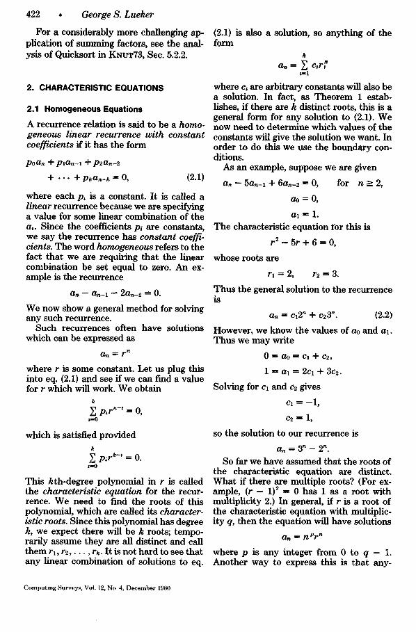
2. CHARACTERISTIC EQUATIONS

2.1 H o m o g e n e o u s E q u a t i o n s

A recurrence re la t ion is said to be a homogeneous l inear recurrence with constant coefficients if i t has the fo rm

poan + plaa-] + p2an-2

+ . ' . + pka , -k = 0, (2.1)

where each p~ is a constant . I t is called a l inear recurrence because we are specifying a value for some l inear combinat ion of the a,. Since the coefficients pi are constants , we say the recurrence has constant coefficients. T h e word homogeneous refers to the fact t ha t we are requir ing t ha t the l inear combina t ion be se t equal to zero. An example is the recurrence

a . - a ~ - i - 2 a n - 2 = 0.

We now show a general m e t h o d for solving any such recurrence.

Such recurrences of ten have solutions which can be expressed as

a n = r n

where r is some constant . Le t us plug this into eq. (2.1) and see if we can find a value for r which will work. We obtain

k

~ p , r~ - ' = 0,

which is satisfied provided

k pir k-~ = O.

This k th -degree polynomia l in r is called the characteristic equat ion for the recurrence. We need to find the roots of this polynomial , which are called its characteristic roots. Since this polynomial has degree k, we expect there will be k roots; t empo- rari ly assume they are all distinct and call t h e m rl , r2 . . . . , rk. I t is no t ha rd to see t h a t any l inear combina t ion of solutions to eq.

(2.1) is also a solution, so anyth ing of the fo rm

k

an ffi ~ c , r , ~

where c, are a rb i t r a ry cons tants will also be a solution. In fact, as T h e o r e m 1 establishes, if there are k dist inct roots, this is a general fo rm for any solution to (2.1). We now need to de te rmine which values of the cons tan ts will give the solution we want. In order to do this we use the boundary conditions.

As an example, suppose we are given

an - 5an-1 + 6an-2 ffi 0, for n >_ 2,

ao = 0,

a l l 1.

T h e character is t ic equat ion ibr this is

r 2 - 5r + 6 = 0,

whose roots are

r 1 = 2 , r 2 = 3 .

T h u s the general solution to the recurrence i s

an ffi c12" + c23". (2.2)

However , we know the values of ao and a , . T h u s we m a y wri te

0m~" ao f f i C1-[- C2,

1 = a , -- 2c, + 3c2.

Solving for Cl and c2 gives

c, = - I ,

c2-- 1,

so the solution to our recurrence is

an ffi 3 n - 2 n.

So far we have assumed tha t the roots of the character is t ic equa t ion axe distinct. W h a t if there are mul t ip le roots? (For example , (r - 1) ~ ffi 0 has 1 as a root wi th mult ipl ic i ty 2.) In general, if r is a roo t of the character is t ic equat ion with multiplic- i ty q, t hen the equat ion will have solut ions

a n = nPr ~

where p is any integer f rom 0 to q - 1. Ano the r way to express this is t h a t any-

Computing Surveys, Vol. 12, No 4, December 1980

Some Techniques for Solv ing Revurrettees

thing of the form

a~ = (a polynomial in n of degree(2.3) less than q) r =

is a solution. One might wonder whether there are also other solutions not of the form shown in {2.3}. The answer is no, as the following theorem shows.

Theorem 1

Let f (x) be the characteristic equation of the recurrence

poa , + p~a~-~ + p2a,-2 + . . • + pkan-k ffi O,

for n >_ k, (2.4)

where the p, are constants. Le t the roots of f, over the complex numbers, be r,, i ffi 1, . . . . m, and let their respective multiplici- ties be q~, i ffi 1 , . . . , m. Then any solution to (2.4) is of the form

/ q.-1 )

where the % are constants.

We omit the proof here; the interested reader may consult LIu68, App. 3-1. Note tha t in order for the theorem to be true, it is impor tant tha t we determine all of the roots, including those tha t are complex. All of the characterist ic equations discussed in this paper have only real roots. Complex roots, which can give rise to solutions with periodic behavior, can be handled by the methods discussed here, but it is often useful to express such solutions in terms of the sine and cosine functions [LIu68, pp. 62-64].

We now give an example of a recurrence whose characteristic equat ion has a multi- pie root. Le t the rank of a node in a t ree be one more than its number of descendants. (We count a node as one of its own descendants.) When discussing a type of t ree known as a BB(a) tree (see REIN77, Sec. 6.4.3), the notion of the rank of a node can be useful. In particular, sometimes it is useful to find the sum of the ranks of all of the nodes in the tree. This sum is also closely related to the internal and external pa th length of a tree, discussed in KNUT68,

° 423

Sec. 2.3.4.5. Here we determine the total rank an of the nodes in a perfect binary t ree of height n. First note tht/t the rank of the root is 2 TM, since we have M]ceady seen tha t it has 2 "+~ - 1 descendants. T h e total rank of the nodes in each of its subtrees is a~-~. Thus

a ~ - 2 a ~ - 1 f f i 2 n+l ,

aoffi2.

Now unfor tunate ly this is not a homogeneous equat ion because of the ,2 =+1 appear- ing on the r ight-hand side. Shor t ly we will see a systematic way of dealing with such problems, bu t for the t ime being we use an ad hoc approach to force the equat ion to be homogeneous. Note tha t the r ight-hand side doubles each t ime n increases by one. Thus if we take one equat ion and subtract twice the previous one, we can eliminate r ight-hand side, as follows:

a= - 2an-1 ffi 2 n+l - 2 ( a ~ - i - - 2 a a - 2 = 2 ~)

an - - 4a~-1 + 4an-2 = 0

Since this new equat ion is valid only for n _> 2 we must provide a boundary value for al (which we may determine from the recurrence), so the set of boundary conditions becomes

a0 ffi 2, al ffi 8.

The characteristic equat ion is

r2--4r+4ffiO.

This can be rewri t ten as

(r - 2) 2 ffi 0,

so 2 is the only root bu t it occurs twice. Thus the general solution is

a~ ffi (cl + c2n)2 ~.

Using the boundary conditions we obtain

2 = aoffi cl,

8 = a~ ffi 2(c~ + c2).

Solving gives

cl ffi 2, c2 ffi 2,

so the general solution is

a , , - - ( 2 n + 2)2 ~.


~ ~:..:: ....... ~ - : & ~ ' ~ . . . . . .

424 . George S. Lueker

2.2 Nonhomogeneous Equations

We have now seen how to solve any homogeneous linear recurrence with constant coefficients. Often however the recurrence we wish to solve is not homogeneous, as, for example, in

an-5an_ l+6an_2f f i4 , for n _ 2 ,

ao = 5, (2.5)

a l = 7.

A recurrence which looks like eq. (2.1) but has a nonzero function of n on the right- hand side is called anonhomogeneous linear recurrence with constant coefficients. Any sequence an which satisfies the recurrence (but not necessarily the boundary conditions) is called a part icular solution; any sequence which makes the left-hand side identically zero is called a homogeneous solution. Sometimes we can guess a particular solution, but cannot easily find one which makes the boundary conditions hold. In this case the following theorem is very helpful.

Theorem 2 I f we start wi th any part icular solution a, and add any homogeneous solution, we obtain another part icular solution. More- over the difference between any two particular solutions is always a homogeneous solution.

(The proof is easy; we do not present it here.) This theorem suggests the following approach to solving nonhomogeneous recurrences.

1. Guess a particular solution an. 2. Write a formula for a, plus the general

homogeneous solution {with unknown constants).

3. Use the boundary conditions to solve for the constants.

We now demonstrate this technique on the recurrence in (2.5). First we guess a particular solution; after some effort we discover that an = 2 will work. (This process of trying to guess a solution could be quite frustrating. Fortunately there is a systematic method which covers many cases,

and which we discuss in a moment.) We have seen before (2.2) that the homogeneous solution has the form

an = e l 2 n + c23 n.

Thus by Theorem 2 the solution to (2.5) must have the form

an = 2 + c12 n + c23 n.

Solving for the constants using the boundary conditions we obtain

Cl f f i 4, c2 = -1, SO

an ffi 2 + 4 . 2 , , - 3, , .

The method outlined has an obvious dis- advantage: It requires that we be able to guess a particular solution. It would seem much more desirable to have a systematic method for producing particular solutions. We now outline a systematic method which applies to many recurrences. Some additional notation is useful. We represent a sequence by simply writing down a formula for its nth element in angle brackets, assuming elements are numbered starting at 0. For example, the sequence 1, 2, 4 . . . . is represented by (2n). (Be sure to read this carefully; (a,,) denotes a sequence, not the single element an.) Let E be an operator which transforms a sequence by throwing away its first element. For example, the sequence 1, 2, 4, 8, . . . is transformed by E into 2, 4, 8, 16 . . . . . This can be abbreviated by writing

E(2 n) ffi ( 2 n + ~ ) .

In general,

E(a,,) = (an+l).

We can build new operators by combining E with itself and with constants. To do this, for any constant c we define an operator (also denoted by c) by the equation

C(an) = (ca,,).

We also define addition and multiplication of operators by

(A + B)(an) = A(a, , ) + B(a, ,) ,

and

( A B ) ( a , ) = A(B(an) ) .

Comput ing Surveys, Vol 12, No. 4, l )ecember 1980


TABLE 1. ANNIHILATORS FOR VARIOUS SEQUI~NCES

Sequence Annihi lator

(c) E - 1 (a polynomial in n of degree k) (E - 1) k+l (c n) (E - c) (c n times a polynomial in n of degree k) (E - c) k+l

• 425

With these definitions we can easily verify tha t addit ion and mult ipl icat ion of operators are commuta t ive and associative; moreove r mult ipl icat ion distr ibutes over addition. (In fact, the set of all possible opera tors tha t can be constructed as described above forms an algebraic s t ructure known as a Euclidean ring. See HERS64, p. 104.) Here are two examples of applicat ions of operators .

(2 + E)(a, , ) = (2a,, + an+i),

E3(an) = (an+3).

Such opera tors enable us to express certain concepts very concisely. Note, for example, t ha t if f (r) is the characteris t ic polynomial of some recurrence of the form in (2.4), we m a y write the recurrence as

f ( E ) ( a , ) = (0).

As this equat ion suggests, somet imes a certain operator , when applied to a certain sequence, produces a sequence consisting entirely of zeroes. In this case we say tha t the opera tor is an annihilator for the sequence. For example, E - 2 is an annihilator for (2"), since

(E - 2)(2 n) -- (2 n+~ - 2.2") ffi (0).

We can now finally describe a fairly general technique for producing solutions to nonhomogeneous equations with constant coefficients.

1. Apply an annihi la tor for the r ight-hand side to bo th sides of the equation.

2. Solve the result ing homogeneous equa- t ion by the methods discussed earlier.

A list of sequences and corresponding annihilators is shown in Tab le 1. One can prove tha t this table is correct as follows. I t can easily be shown tha t if we apply (E - c) to (c~p(n)), where p(n) is a polynomial of posit ive degree d, we obtain (c"q(n)), where q(n) is a polynomial of

degree d - 1. Using this and an easy induc- tion, we can establish tha t the last line in the table is correct. All of the o ther lines are special cases of the last line.

One can easily prove t h a t ff A is an annihi la tor for (an) and B is an annihi la tor for (bn), then the product AB is an annihi lator for the sum (a, + b,). Thus, for example, an annihi la tor for (n2 n + 1) is (E - 2)2(E - 1).

We now work out two examples. T h e first is eq. (2.5), which we solved above by guess- ing the par t icular solution. With our new nota t ion we can write this as

( E 2 - 5E + 6)(an) = (4).

Factoring gives

(E - 2)(E - 3)(an) ffi {4).

Now apply (E - 1) to annihilate the 4.

( E - 1 ) ( E - 2 ) ( E - 3 ) ( a n ) ffi ( 0 ) .

This has the character is t ic equat ion

(r - 1)(r - 2)(r - 3) ffi 0,

with distinct roots 1, 2, and 3. T h u s we mus t have

a , -- cl + c22 n + c,~3 ~.

We can solve for the constants by noting tha t

a 2 - 5 a l + 6 a o ffi 4 ,

aoffi5,

al •7 .

T h e result is

an ffi 2 + 4 .2 n - 3 n,

as before. For a second example, consider the equa-

t ion an - 2an-1 -- 2 n - 1, for n ~- 1,

ao ffi 0. (2.6)

Computing Surveys, Vol. 12, No. 4, I)ecember 1980


(We show an impor tant application of this recurrence in Section 3.) Using the operator E we ma y write

( E - 2 ) { a . ) = ( 2 "+1 - 1 ) .

T h e annihi lator for the r ight-hand side is (E - 2)(E - 1), so we obtain

( E - 1 ) ( E - 2 ) 2 ( a . ) = (0).

Thus the characteristic roots are 2 (with a multiplicity of 2) and 1, so

a n = (Cl 4" c 2 n ) 2 n 4- c3.

Solving for the constants we obtain

cl ffi - 1 , c2 -- 1, c3 ffi 1, SO

a n ffi (n - 1 ) 2 n 4- 1 .

3. DOMAIN AND RANGE TRANSFORMA- TIONS

Somet imes it is useful to apply a transfor- mat ion to a sequence in order to make it appear in a more desirable form. A sequence can be thought of as a mapping from the integers into the reals; thus we call a t ransformation on the values of the sequence a range t rans format ion and a t ransformat ion on the indices a domain transformation. (In LEVY61, p. 103, sequences which can be t ransformed by domain or range transformations into linear recurrences are called "pseudo-non-l inear equations.") We begin by showing an example of a range transformation. Suppose

a n = 3a2-1, for n _> 1,

a0f f i l .

This cannot be solved by any method discussed so far, but if we let

b, = l g a ,

(where lg denotes the base-2 logarithm), we m ay rewrite the recurrence as

b, = 2b,-1 + lg 3,

b 0 = 0 .

This can easily be solved by the methods discussed before. The result is

b, = ( 2 " - 1) lg 3,

s o

a n = 2 (2n-1)ig 3 ~_ 32"-1.

Next we show how domain transforma- t ions can be useful. Recall the recurrence which we ment ioned at the beginning of this paper for Mergesort:

T(n) = 2T(n /2 ) + n - 1,

for n >_ 2, (3.1)

T(1) = 0,

where n is required to be a power of 2. (See AHO74, pp. 65-67.) We may be t empted to consider the recurrence

a n = 2an~2 + n - 1,

but none of the techniques we have discussed so far are directly applicable to this equation. However if we let

n = 2 k and ah ffi T(n) ffi T(24),

we can write

ak = 2ak-1 + 2 4 - - 1, for k _> 1,

a o = 0 .

Th is is a recurrence which can be solved by the methods already described. In fact, it is one of those which we solved as an example in the preceding section, namely (2.6). T h e solution we found was

ak = (k - 1) 24 + 1.

Thus, since a~ = T(24), we may conclude tha t

T(n) f f i ( l g n - 1 ) n + l .

Next we give an example of a more difficult domain transformation. I t is possible to mult iply two n-bi t numbers by doing three multiplications of (n/2 + D-bit (or shorter) numbers and O(n) additional work. (See AHo74, pp. 62-65; there the algori thm is described in a way which needs only mult iply n /2-bi t numbers, bu t a more natural implementa t ion yields the recurrence we are about to analyze.) Applying this decomposit ion recursively (and stop- ping the recursion when the numbers are of length 3 or less) leads to an algori thm whose complexity is described by

T(n) = 3 T ( n / 2 + 1) + O(n),

for n > 3 , (3.2)

T(3) ffi O(1).

S o m e T e c h n i q u e s f o r S o l v i n g R e c u r r e n c e s • 427

T h e O-nota t ion in the recurrence is a little inconvenient . To el iminate it, note tha t there mus t be some constant c' such tha t the extra t ime represented by the " O ( n ) " in the recurrence is bounded by c'n. Simi- larly, there is a constant c" such tha t the t ime represented by the "O(1)" is bounded by c". Lett ing c be the larger of these, we conclude tha t we m a y bound T(n ) by 1'(n), if ~/'(n) is the solution to

~(n) = 3 ~ ( n / 2 + 1) + c n,

for n > 3 , (3.3)

~ ( 3 ) = c.

Since we only seek the O-notat ion for the complexi ty of the algori thm, we can scale this by any constant factor. In par t icular we m a y let c be 1, to obtain

~(n) -- 3~/'(n/2 + 1) + n,

for n > 3 , (3.4)

~'(3) ---- 1.

We would like to be able to choose an index k so tha t the recurrence could be wri t ten as

ak = 3ak-~ + (some function of k). (3.5)

Let nk denote the value of n corresponding to a given k. In order for (3.4) to correspond to (3.5), we mus t have

nk-1 ffi nk /2 + 1,

SO

nk = 2nk-1 -- 2.

We call this a s e c o n d a r y r e c u r r e n c e for (3.4). I f we let no = 3, the solution is

nk = 2 k + 2.

Now if we let

ak -- ~(nk),

we may rewrite (3.4) as

ak --- 3ak-~ + 2 k + 2,

ao ffi l .

Solving this yields

ah ffi 4 .3 k - 2.2 k - 1.

Since the relat ion be tween n and k implies

k ffi lg(n - 2),

we conclude t ha t for any n which appea r s in the sequence ( n D ,

~(n) ffi 4 .3 igor-2) - 2 .2 Igor-2) - 1

ffi 4(n - 2 ) lg3 - 2(n - 2) - 1

ffi 4(n - 2 ) i g3 - 2n + 3.

T h u s this me thod for mult iplying two numbers works in T ( n ) ffi O(n I¢~) time. Since lg 3 is abou t 1.59, this mult ipl icat ion me thod is asymptot ica l ly fas ter t han the s imple O(n 2) approach.

For very large n a m u c h fas ter way of mult iplying n-bi t numbe r s is the Schon- hage-S t ras sen me thod [AHo74, Sec. 7.5; SCHO71]. In analyzing this me thod the following recurrence arises.

T ( n ) ffi lg n + 2T(4 nl/2). (3.6)

We begin the solution of this recurrence by using a domain t ransformat ion. T h e appro- pr iate secondary recurrence is

A ~1/2 n t ~ ~ i$i+1.

T o convert this into a more t rac table form, we m a y use the range t rans format ion m, ffi lg n,. T h e n we have

m~ ffi 2 + m,+~/2.

This can be solved by the me thods of Sec- t ion 1 or Sect ion 2. T h e solut ion is

m, ffi 2 t + 4, SO

n~ ~- 2 ~+4. (3.7)

(Other solutions are also possible since we have not s ta ted the boundary conditions.) I f we now let a, ffi T(nl ) , eq. (3.6) becomes

a, -- 2' + 4 + 2a,-1,

which is readily solved to yield

a~ ffi i2 ' + b2' - 4,

where b is unspecified since we have not given boundary conditions. T h e n since f rom {3.7)

= lg ( lg n, - 4) ,

it mus t be t ha t for any n appear ing in the sequence (n~),

M ( n ) ffi O(i2 i)

--- O(lg(lg n - 4) 2 ( lg ( lgn-4) ) )

= O ( l g ( l g n - 4 ) ( l g n - 4 ) )

ffi O ( l g n lg lg n) .


428 • George S. L u e k e r

TABLE 2. G~.NERATING FUNCTIONS FOR SOME S E Q U E N C E S

Sequence Generating Function

1, 1, 1, I , . . . 1, C, C 2, . . .

1, 2c, 3c2 , . . . , (i + 1)c',...

(o) (:) ..... (:) ....

I'bZ+Z2"i'Za4" . . . . 1 / ( l - - z )

1 + cz + (cz) 2 + . . . = 1 / (1-cz ) 1 / (1-cz ) ~

(1 + z)"

Using this solution one can show that the SchSnhage-Strassen algorithm will multiply two n-bit numbers in O(n lg n lg lg n) time; see AHo74, Sec. 7.5, for more details.

4. GENERATING FUNCTIONS

4.1 Generating Functions for Sequences

Generating functions are an ingenious method by which certain problems can be solved very elegantly. Like Laplace transforms and Fourier transforms, generating functions transform a problem from one conceptual domain into another, in the hope that the problem will be easier to solve in the new domain.

Definition

The g e n e r a t i n g func t ion for the sequence a0, al, a2 . . . . . is the function

ao

A ( z ) = ~ a,z'. t--O

(The sum in the definition might not always converge; we have more to say about this later. In FELL68, Sec. XI.1, the definition given for generating functions requires that the series converge over some interval of positive length.) At first there seems to be little motivation for the definition of generating functions, but we shall see that certain types of operations on sequences correspond to certain other operations on generating functions. Thus in tackling a problem we can choose whichever domain makes the problem easier. Table 2 provides some examples of sequences and corresponding generating functions. Note that if n is a positive integer, the last generating function is a polynomial. We can extend the

Computing Surveys, Vol 12, No. 4, December 1980

usefulness of this generating function by using an extended definition of the binomial coefficients, as in LIu68, Sec. 2-2, and S~.DG75, p. 299. For any real n and any integer i define

= i f i < 0 t h e n 0 e l s e I ~ ° (n - j ) .

Then the last line in the table is valid for any real n and gives a sequence with infi- nitely many nonzero values if n is negative or nonintegral.

Now we show how some standard operations on functions correspond to operations on sequences. (Further discussion of these operations can be found in KSUT68, Sec. 1.2.9, and REXN77, Sec. 3.3.) Let A ( z ) and B ( z ) be the generating functions for (a,) and (b,) respectively. In Table 3 the left column shows a function that can be obtained from A and B by simple operations and the right column shows a formula for the ith element of the corresponding sequence.

We now show how generating functions can be used to solve a simple recurrence. Suppose that

a . -- 2an-1 + 1,

a o = l.

Let

for n > 1,

a~

A ( z ) = ~ a . z" . n~O

From the recurrence, this sum can be re- written as

oo

A ( z ) ffi 1 + ~ (2a,=-1 + 1)z" n - -1

oo oo

= l + z ~ 2a.-1 + ~ z" n - -1 n - - I

(11) • l + 2zA( z ) + '1 z

Note what has happened. Initially we had a problem to be solved for (a.). In the left and right sides of the foregoing equation we have a problem which is to be solved for .4. This new problem is a simple one. Algebra yields

1 A ( z ) =,

(1 -- z ) ( 1 -- 2 z ) "


TABLE 3. OPEEATmNS ON GENERATING FUNCTIONS

Generating Formula for tth Functwn Element of Sequence

cA ca, A + B a, + b, AB Y,~-o a~b,_j

zkA(z) i f i < k t h e n 0 else a,-k

A(z) 1 - z Y~-o at zA'(z) ia~ S ~ A(t) dt i f i = 0 t h e n 0 e lse a,-1/~

Now we must return to the original problem domain. Unfortunately A(z) is not in Table 2. However, by use of partial fractions, we may write

1 -1 2

( 1 - z ) ( 1 - 2 z ) 1 - z 1 - 2z

(We do not discuss here the problem of decomposing a rational expression with partial fractions; the interested reader may consult FADE64, Sec. 13.8.) Using Tables 2 and 3, we now see that the corresponding sequence is given by

an = 2 "+1 - 1.

This agrees with the solution in eq. (1.8). At this point a word of caution is in order.

We have done some formal manipulations involving sequences but have ignored ques- tions such as convergence. This might lead to extraneous answers in some cases. There are at least two possible ways to avoid difficulty. One approach is to check the answer by some independent method. In our example a simple inductive proof would suffice. A second approach is to check carefully the validity of each step. In our example we could tell by inspection of the recurrence that

lim an+l ~- 2, n--)oo a n

and hence that the radius of convergence of A(z) is ½ (by BUCK78, Th. 14, p. 240). This could form the basis of a rigorous proof of the validity of our operations. (See also the discussion in KNUT68, Sec. 1.2.9. For a good rigorous discussion of properties of series, see BUCK78, Chaps. 5 and 6.) In the remainder of this paper we do not always perform these verifications.

° 429

As a second example of the use of generating functions, we consider the problem of counting the number of distinct binary trees with a given number of nodes. (We assume that the nodes are indistinguish- able. Thus we consider two trees identical if they have the same shape. This is sometimes referred to as the enumeration of planted plane binary trees.) This example shows that generating functions can be used to solve problems for which the techniques of Sections 1 and 2 do not seem to be of much help. Let bn be the number of distinct binary trees which can be formed from n nodes; let B (z) be the generating function for (bn).

Before continuing the analysis it is worth noting that the generating function must converge for any z in the open interval (-¼, ¼). To see this let the type of a node be 0 ff it has no children, 1 if it has only a left child, 2 if it has only a right child, and 3 if it has both children. It is not difficult to show (see STASS0, Sec. 3.5.2) that if we have a list of the types of the nodes in preorder, then we have enough information to reconstruct the tree. Now there are only 4" strings of n of these four types; thus it must be that bn - 4 n. Hence the radius of convergence of B (z) must be at least ¼.

To get more information about B (z) we determine a recurrence for (bn). A binary tree on one cr more vertices has to have a root. Assuming it has n + 1 nodes, the remaining n nodes can be distributed arbi- trarily between the left and right subtrees. Note that if we put i nodes in one subtree there will be n - i nodes remaining for the other tree. If we choose to partition the nodes this way, we can still build the left subtree in any of b, ways and the right subtree in any of bn-, ways, for a total of b~bn-, combinations. Summing over all the possible choices for i, we come up with the following recurrence.

n

bn+l = ~ b,bn-,, for n _> 0, ~=0 (4.1)

b0 ~ 1.

The boundary condition may seem a tittle strange at first. We need this for con- sistency, however, since if we decide to put



all of the nodes in the one subtree there is exactly one way to build the other subtree, namely, to put nothing there.

To begin to convert eq. (4.1) into a statement about B(z ) , we multiply by z n and sum as n goes from 0 to infinity.

2 b,+l z n = ~, b,bn_,Z n. (4.2) n--O n--O t~O

The left side of (4.2) is

bl + b2z + b3z 2 + b4z a + . . . .

This is just the same as B(z), except that we have deleted the first term (b0) and removed one factor of z. Therefore, since bo is 1, the left side is

(B(z) - 1)/z.

The right side, from the third line of Table 3, is

B(z) 2.

Thus {4.2) becomes

(B(z) - 1)/z = B ( z ) 2,

which can be rearranged as

zB( z ) 2 - B ( z ) + 1 = O,

and solved by the quadratic formula to obtain

1 __. ~ f l - 4z B(z) = (4.3)

2z

At this point we might be a little dismayed, since the _+ sign gives two solutions, and it is not apparent which is correct. However note that

B(0) ffi bo + blz + b2z2 + . . . Iz-0 ffi b0.

Thus B (0) must be 1. Now if we choose the - sign in (4.3), B(0) will indeed be 1; ff we choose the + sign, B(z ) approaches infinity as z approaches 0. Thus we may finally conclude that

1 - ~/1 - 4z B(z) ffi (4.4)

2z

A number of texts have shown how to obtain an exact formula for bn from this generating function [KNUT68, Sec. 2.3.4.4;

STAN80, Sec. 3.3.2; REIN77, Sec. 3.3]. It is shown that

n +----~ " (4.5)

We do not repeat this part of the solution here. However, at the end of the third part of our discussion of generating functions, we show how to obtain an asymptotic de- scription of b, very easily.

4.2 Probability Generating Functions

Let X be a random variable which assumes nonnegative integer values and letp, be the probability that X = i. Then the probabi l i ty genera t ing funct ion (pgf) for X is the generating function for (p,). Note that its radius of convergence must be at least 1, since probabilities lie in the range [0, 1]. Such functions have some particularly nice properties, which we explore in this section.

Suppose X and Y are two independent nonnegative integer random variables, with probability generating functions P and Q respectively. Using the third line in Table 3, we can readily establish the rather pleas- ing fact that the pgf for the sum of X and Y is the product of P and Q. (It must be stressed that this fact is not true i fX and Y are not independent. As an extreme example, note that the pgf for X + X is P(z2), not (P(z))2.)

Many of the commonly encountered nonnegative integer random variables have easily expressed generating functions. A few of these are summarized in Table 4. (This table is based on FELL68, Sec. XI.2.) The first two distributions can be described in terms of a sequence of flips of a biased coin, which lands heads up with a probability of p. The binomial distribution tells the number of heads in n flips. The geometric distribution describes the number of tails that occur before the first head. The Poisson distribution can be viewed as a limiting case of the binomial distribution, in which we let n --~ ~ and p --+ 0 in such a way that p = )~/n. Radioactive decay provides a simple example of such a distribution. If we assume that decays of separate atoms are independent, then the number of flashes of a radioactive watch dial in some time period has very nearly a Poisson distribution. By tak-


TABLE 4.


PROBABILITY GENERATING FUNCTIONS FOR SOME RANDOM VARIABLES

Probabdity Name Formula for pk Generattng Function

Binomial (~) pk(1- p)'-k (1-p+Pz)n

Geometric pqk 1 - q where q = 1 - p 1 - qz

Poisson k~e-~'/k! e ~(~-l)

• 4 3 1

ing the limit of the generating function for the binomial distribution and invoking the Continuity Theorem, we can obtain the generating function shown in the table for the Poisson distribution; see FELL68, Sec. XI.6.

Another useful property of probability generating functions is that they enable us to find certain expected values quickly. (See FELL68, Sec. IX.2, for a discussion of expectation.) For example, note that

ov

P'(1) = ~ ip, ffi E[X].

Table 5 presents a number of formulas for expected values; Dz denotes the derivative with respect to z. (The first three lines of the table may be found in FELL68, Secs. XI.1 and XI.2, and KNuT68, Sec. 1.2.10. The fourth line follows easily from line 6 of Table 3.)

Some caution must be exercised when using Table 5. We express the possible problem in terms of the last line, since the first three lines are special cases of it. Let r be the radius of convergence of the generating function. If ] c I > r, the function in the left column does not have a finite expectation, even though the formula in the right column may seem to give an answer. In the case c ffi r, a finite expectation may or may not exist. In this case if c > 0 and

lira (zD~) kP(z) z~c

exists, then a finite expectation does exist and is given by the limit. If lc [ < r, the formula always gives the correct answer. Note that for the binomial and Poisson distributions the generating function con- verges everywhere, so problems of the sort discussed here do not arise.

As an example of the application of probability generating functions we now analyze

the expected complexity of a highly efficient sorting algorithm known as address calculation sorting [ISAA56; KNUT73, Sec. 5.2.1]. Suppose we know that the data to be sorted (xl, x2, . . . , x,) are distributed uniformly and independently over the open interval (0, 1). The following algorithm clas- sifies the data into n buckets, each corresponding to a piece of the interval of length 1/n. Then it sorts each bucket and concate- nates them. The hope is that each bucket will contain so few elements that each sort can be performed in very little time.

begin f o r k :-- 0 u n t i l n - I d o

Lk :-- the empty list; f o r ~ :ffi I u n t i l n d o

begin k :ffi f loor(nx~); "append x, to Lk;

e n d ; f o r i :ffi 0 u n t i l n - I d o

if L, is nonempty then sort Li b y insertion sort;

output Lo II L~ [I L2 [[ . . - [I L~-I; e n d ;

Here two consecutive vertical bars denote concatenation of lists.

Aside from the time in the sorts, the algorithm clearly uses O(n) time. We show that the expected time for each sort is O(1) and hence the overall time is O (n).

First we determine the generating function for the length X of one of the lists, say L0. Note that each element, independently, has a probability of 1/n of being placed into list Lo. Since there are n trials we obtain a binomial distribution. From Table 4, ff we let p -- 1/n, X has the generating function

P(z) f f i ( 1 - p + P z ) n f f i ( l + Z - 1 ) n ' n

The time to perform insertion sort is O (X2).

Computing Surveys, VoL 12, No. 4, December 1980

432 • George S. L u e k e r

TABLE 5. EXPECTED VALUES FOR SEVERAL FUNCTIONS OF A RANDOM VARIABLE X WITH

PROBABILITY GENERATING FUNCTION P

Function of X Expected Value

X P'(1) X 2 P"(1) + P'(1) c X P(c) X% x (zDz)kP(z) ]z-c

But by Table 5,

E [X 2] -- P"(1) + P'(1)

- n - l ( l + Z - 1 ) n - 2 n n

.(l.Z 7' I n z - i

R - - 1 - - - - b l < 2 .

n

Thus the expected time for each sort is iIldeed O(1), so this sorting algorithm runs in O (n) time under the given assumptions.

This same type of problem arises in a different context in an analysis of the traveling salesman problem [KARP77]. There is a well-known dynamic programming approach which yields an O(n~2 n) algorithm for this problem [BELL62, HELD62]. In KARP77, this is used as one of the building blocks for an algorithm which tends, asymptotically, to run quite quickly and give near-optimal results on the average, under certain assumptions about the distribution of inputs. In particular it is assumed that the number of points is drawn from a Poisson distribution with mean n, and that the points are distributed uniformly over the unit square. The square is subdivided into subsquares and the TSP is solved op- timally for the set of points within each subsquare. These solutions are then com- bined to produce an approximate solution for the entire problem. Part of the analysis involves determining the average amount of time spent solving one of these subproblems. If each subsquare has area A, then the number of points within each subsquare has a Poisson distribution and a mean of A n . Let X denote a variable with this distribution, and, for convenience, let m = A n . Thus to evaluate E [ X 2 2 x]

we write

(zDz)2em(z-1)[z.2 f f i (zDz)zmem(Z-1) l z . 2

ffi (4m 2 + 2m)e m ffi O(m2em).

Note that if the number of points were exactly m, the time used would be O(m22 m) rather than O(m2em). Since the function m22 m grows rapidly, the effect of the fluc- tuation of X about its mean is to increase the mean time somewhat.

As a final example of an application of probability generating functions, we consider the problem of solving a random assignment problem. Donath [DONA69] used generating functions in obtaining a lower bound on the average value of the optimum solution. We discuss his argument here. To define the assignment problem assume that a manager must assign n workers to n jobs, and that we have a matrix (c~) in which c,~ indicates how much worker i dislikes job j. The manager wishes to assign workers to jobs so as to minimize the total worker dissatisfaction. More formally, he wishes to choose exactly one element from each row of the matrix in such a way as to minimize the total of the selected elements. We call this minimum total the va lue o f the opti- m u m solut ion. Donath showed how to obtain a lower bound on the average value of the optimum solution for a random matrix. Of course, in order to make this precise, we must state the assumptions to be made about what a "random matrix" looks like. In the result reported here Donath assumed that each row was (independently) a random permutation of the integers from 1 to n; each of the n! permutations could occur with equal probability. (See GONN79 for an interpretation of the assignment problem, with this distribution of inputs, in terms of ideal structuring of hash tables.) To begin, we fix one possible assignment and try to find the pgf for the sum it yields for a random matrix. Note that in each row this assignment yields, with equal probability, a number from 1 to n. Thus the pgf for the number selected from any particular row is

z + z ~ + . . . + z n z ( 1 - z n)

n n(1 - z) "

Computing Surveys, Vol. 12, No 4, December 1980

Some Techniques for Solving Recurrences • 433

To find the pgf for the total cost of the n rows, we merely raise this generating function to the n th power to obtain

z"(1 - z~)"

n~(1 - z) ~

It will turn out that we are more interested in the cumulative probabilities, that is, the sequence (ak) where ak is the probability that the total is less than or equal to k. To obtain this, we apply the summation operator found in line 5 of Table 3, namely, 1/(1 - z), to obtain

n-~z"(1 - z)-(n+l~(1 - z~) ". (4.6) Now, as we verify in a moment, the range of k over which we need the values of ak is n < k < 2n. An inspection of (4.6) shows that for k in this range, the coefficient of z k must be the coefficient of z k-" in

n-~(l - z)-("+l).

By an application of the binomial theorem we can establish that this coefficient is

( - 1 ) n - k n - ~ ( - ; 2 : ) ) ffi n -~(k k n ) ,

where the equality follows from SEDG75, identity (16), p. 301.

So far we have been considering the probability that the total cost is bounded by k, given a fixed assignment of columns to rows. To bound the optimum, we must bear in mind that n! assignments are possible. Now by Boole's inequality the probability that any of the assignments yields a cost bounded by k is no more than the sum, over all assignments, of the probability that this particular assignment does. Thus if we let bk be the probability that the optimum is less than or equal to k we have

b k < n ! a k = n ! n - n ( k ) - - k - n " (4.7)

Using Stirling's approximation one may establish that

in b, <_ n[fl ln fl - (fl - 1) In ( f l - 1) - 1]

+ O(ln n),

where k = fin. Now let fl0 be the root of

f l l n f l - ( f l - 1 ) i n ( f l - 1 ) - l = 0 . (4.8)

It is not hard to establish that if fl < rio, the

right-hand side of (4.7) approaches 0 expo- nentially as n approache~ infinity. From this we may deduce that the average value of the optimum is asymptotically bounded below by Bon. Numerical solution of (4.8) reveals that P0 is about 1.54221. Simulation of the assignment problem with random data of the type discussed here suggests that actually the optimum tends to be asymptotic to approximately 1.8n [DONA69, GONN79]. Thus this lower bound is proba- bly not tight. See WALK79 for a derivation of an upper bound for a very closely related problem.

4.3 Extracting Asymptotic Information from Generating Functions

In this subsection we briefly discuss the problem of determining the asymptotic behavior of the sequence (an) from its generating function A(z). For this subsection only, the reader needs familiarity with complex variables and with the gamma function. In BEND74 a number of useful techniques are presented, along with numerous interesting applications. Here we discuss one of the theorems from that paper, which can be applied to many generating functions. We apply it to the generating function for the number of binary trees on n nodes, which we showed in (4.4) to be

1 - ~/1" - 4 z B(z) = (4.9)

2z

If a function f has a singularity at a, we say it is an algebraic singularity if near we can write f as

g(z) f(z) ffi fo(z) + (4.10)

(1 - z / a ) ~

where fo and g are analytic near a, g is nonzero near a, and w is not 0, -1, -2, . . . ; we assume here that w is real. The following theorem is stated (in a slightly different and more general form) in BEND74, Th. 4, p. 498, as a special case of Darboux's Theorem [Sz~659, Th. 8.4, p. 205].

Theorem 3 [BEND74, SZEG59] Suppose that for some real r > O, A(z) is analytic in the region [ z I < r, and has a finite number k > 0 of singularities on the

Computing Surveys, VoL 12, No, 4, December 1980


circle I z I ffi r, al l o f which are algebraic. L e t ai, o~i, a n d g , i ffi 1 . . . . . k, be the values of a, ~, a n d g in (4.10) corresponding to the i-th such singularity. Then A(z ) is the generat ing funct ion for a sequence (an) sat- isfying

1 ~ g,(ai)n '~' J an ~ n ,=1 ~ + °(r-nnw-1 )"

where w is the m a x i m u m of the ¢o,, a n d F denotes the g a m m a function.

Although the statement of this theorem is fairly complex, it can sometimes be applied very easily to give asymptotic information. For example, for the generating function B(z) in (4.9) one easily establishes that

1 r f f i - k f f i l , 4' 1 1 - 1

al = 4 ' wl = - ~, g~(z) --- 2"--z"

Hence by the theorem, 1 - 2n -1/2

b n ~ - - . n F(-½)(¼)"

+ o((¼)-nn -~/~)

4 ~

~r~ n 3 / 2 '

which agrees with the result obtained in KSUT68, Sec. 2.3.4.4; STAN80, Sec. 3.3.2; and REIN77, Sec. 3.3, by applying Stirling's approximation to the exact solution (4.5).

Although we do not reproduce the proof of the above theorem, we mention one of the ideas which is close to the heart of the proof, and which is quite interesting in its own right.

Lemma

Suppose tha t for some real r > O, A(z ) is analyt ic in the region I z I < r a n d continuous for ] z I <_ r. Then A(z) is the generat ing function for a sequence ( an ) satisfy- ing

1 f c A ( Z ) dz an = ~ i Z n+l '

where C is the contour I z [ ~- r, the integra- tion is counterclockwise, and i is the square root o f - 1 .

Computing Surveys, Vol 12, No. 4, December 1980

This formula can be established using the Cauchy integral formula [CHUR60, Secs. 51 and 52], the theorem on Taylor series [CHUR60, Sec. 56], and the fact that A must be uniformly continuous on the closed region bounded by C.

For other examples of the extraction of asymptotic information from generating functions, see BEND74 and HARA73, Chap. 9.

5. SUMMARY

We have discussed the application of recurrences to problems in computer science and surveyed some techniques for solving them. We have also seen how generating functions provide a useful technique for manipulating sequences, including some applications other than the solution of recurrences. Many of the techniques used for dealing with recurrences--for example, annihila- t o r s - a r e similar to those used with differ- ential equations [FADE68, Chaps. 9 and 10].

Many authors have written discussions of sequences, recurrences, and generating functions. MILN60 is a useful text entirely on finite differences; in particular, Chapter XIV discusses methods for solving linear recurrences in which the coefficients are rational functions of n. KNUT68, KNUT73, and Rv.xs77 discuss recurrences in the context of algorithm analysis. HALL67, Chap. 3; LIu68, Chaps. 1 and 2; RIOR58, Chaps. 1 and 2; and RIOR68, Chaps. 1 and 4, discuss them in the context of combinatorial analysis. In SEDG75, which performs a very interesting and thorough analysis of a number of variations of Quicksort, Appendix B provides a useful discussion of recurrences and generating functions, especially as they relate to harmonic numbers and binomial coefficients. For more information on generating functions, see BV.ND74, FLAJ80a, FLAJ80b, LIU68, and STAN78. GONN78 discusses useful methods for obtaining asymptotic estimates of summations. SLOA73 provides a remarkable encyclopedia of various sequences of integers. The reader is en- couraged to consult these references for


some fascinating topics which we have not GONN78 presented here.

ACKNOWLEDGMENTS GONN79

This paper was originally written for use in the ICS 161 and ICS 233 classes at the University of California at Irvine. I am grateful to the members of these classes HALL67 for their comments and suggestions. The referees made many helpful suggestions on the form and con- HARA73 tent of the paper, and brought to my attention the material on asymptotic analysis of generating functions. I am also grateful to Jon Bentley and Denms HELD62 Kibler for their encouragement and suggestions

Preparation of this paper was supported in part by the National Science Foundation under Grant MCS79- HERS64 04997. It was facilitated by the use of MACSYMA, a large symbohc manipulation program developed at the ISAA56 M.I.T. Laboratory for Computer Science and supported by the National Aeronautics and Space Admin- istration under Grant NSG 1323, by the Office of KARP77 Naval Research under Grant N00014-77-C-0641. by the U.S. Department of Energy under Grant ET-78- C-02-4687, and by the U.S. Air Force under Grant F49620-79-C-020. KNUT68

AHO74

BELL62

BEND74

BUCK78

CHUR60

DONA69

FADE64

FADE68

FELL68

FLAJ80a

FLAJ80b

REFERENCES KNUT73

AHO, ALFRED, HOPCROFT, JOHN, AND ULL- MAN, JEFFREY The des~r~ and analysts of computer algorithms, Add~on-Wesley, LEVY61 Reading, Mass., 1974. BELLMAN, R.E. "Dynamic programming treatment of the travelling salesman prob- LIU68 lem," J. A C M 9 (1962), 61-63. BENDER, E.A. "Asymptotic methods m enumeration," SIAM Rev. 16, 4 (Oct. MILN60 1974), 485-515. BUCK, R.C. Advanced calculus, 3rd ed., McGraw-Hill, New York, 1978. CHURCHILL, R. V. Complex variables REIN77 and appheations, McGraw-Hill, New York, 1960. DONATH, W.E. "Algorithm and average- value bounds for assignment problems," RIOR58 IBM J. Res. Dev. 13 (July 1969), 380-386. FADELL, ALBERT G. Calculus with ana- RIOR68 lytw geometry, Van Nostrand, Princeton, N.J., 1964. SCHO71 FADELL, ALEERT G. Vector calculus and differenttal equattons, Van Nostrand, Princeton, N.J., 1968. SEDG75 FELLER, W. An introduction tg probabd- try theory and tts apphcattons, Vol. I, 3rd ed., Wiley, New York, 1968. FLAJOLET, P., FRANQON, J., AND VUILLE- MIN, J. "Sequence of operations analysis SLOA73 for dynamic data structures," J. Algorith. 1(1980), 111-141. FLAJOLET, P., AND ODLYZKO, A. STAN78 "Exploring binary trees and other simple trees," in 21st IEEE Symp. Foundations of Computer Science, Syracuse, N.Y., Oct. 1980, pp. 207-216.

• 4 3 5

GONNET, GASTON H. "Notes on the de* rivation of asymptotic expressions ~om summations," Inf. Process. Lett. 7, 4 (June 1978), 165-169. GONNET, GASTON H., AND MUNRO, J. hN "Efficient ordering of hash tables," SIAM J. Comput. 8, 3 (Aug. 1979), 463- 478. HALL, MARSHALL Combinatorial theory, BlaisdeU, Waltham, Mass., 1967. HARARY, F., AND PALMER, E. M. Graphical enumeration, Academic Press, New York, 1973. HELD, M., AND KARP, R.M. "A dynamic programming approach to sequencing problems," SIAM J. 10 {1962), 196-210. HERSTEIN, I.N. Topics in algebra, Blais- dell, Waltham, Mass., 1964. ISAAC, E. J., AND SINGLETON, R. C. "Sorting by address calculation," J. ACM 3 (1956), 169-174. KARP, R. M. "Probabilistic analysis of partitioning algorithms for the traveling- salesman problem in the plane," Math. Oper. Res 2, 3 (1977), 209-224. KNUTH, DONALD The art of computer programming. Vol. 1: Fundamental algorithms, Addison-Wesley, Reading, Mass., 1968. KNUTH, DONALD The art of computer programming. Vol. 3: Sorting and searching, Addison-Wesley, Reading, Mass., 1973. LEVY, H., AND LESSMAN, F. Flnit~ d~ffer. enee equations, Macmillan, New York, 1961. LIu, C.L. Introduction to combinatorial mathematics, McGraw-Hill, New York, 1968. MILNE-THoMSON, L. M. The calculus of finite differences, Macmillan, London, 1960. REINGOLD, EDWARD M., NIEVERGELT, JURG, AND DEO, NARSINGH Combinato- rial algorithms: Theory and practice, Prentice-Hall, Englewood Cliffs, N.J., 1977. RIORDAN, J. An introduction to combinatorial analysis, Wiley, New York, 1958.

RIORDAN, J. Combinatorial identities, Wiley, New York, 1968. SCHONHAGE, A., AND STRASSEN, V "Schnelle Multiplikation Grosset Zah- len," Computing 7 (1971), 28i-292. SEDGEWICK, ROBER~ "Quicksort," Rep. STAN-CS-75-492, Computer Science Dept., Stanford Univ., Stanford, Ca[if,, May 1975. SLOANE, N. J. A. A handbook of integer sequences, Academic Press, New York, 1973. STANLEY, R.P. "Generating functions," m MAA studies in mathematics. Vol. 17: Studies m combinatorics," Gian-Carlo Rota (Ed.), The Mathematical Association of America, 1978, pages 100-141.


436 * George S. Lueker

STANS0 STANDISH, T. A. Data structure techniques, Addison-Wesley, Reading, Mass., 1980.

SZEG59 SZEGO, G. Orthogonal polynomials, American Mathematical Society CoUo-

WALK79

RECEIVED JUNE 1980; FINAL REVISION ACCEPTED SEPTEMBER 1980.

quium Publications, Vol. 23, American Mathematical Society, Washington, D.C., 1959. WALKUP, D.W. "On the expected value of a random assignment problem," SIAM J. Comput. 8, 3 (Aug. 1979), 440-442.


Documents

Some Techniques for Solving Recurrences - ict.ac.cnbioinfo.ict.ac.cn/~dbu/AlgorithmCourses/Lectures/Lec5-solving... · Some Techniques for Solving Recurrences ... CR Categorws" 5.25,