Capital Asset Pricing Model (CAPM) at Work

• Some of the Intuition behind CAPM

• Applications of CAPM

• Estimation and Testing of CAPM

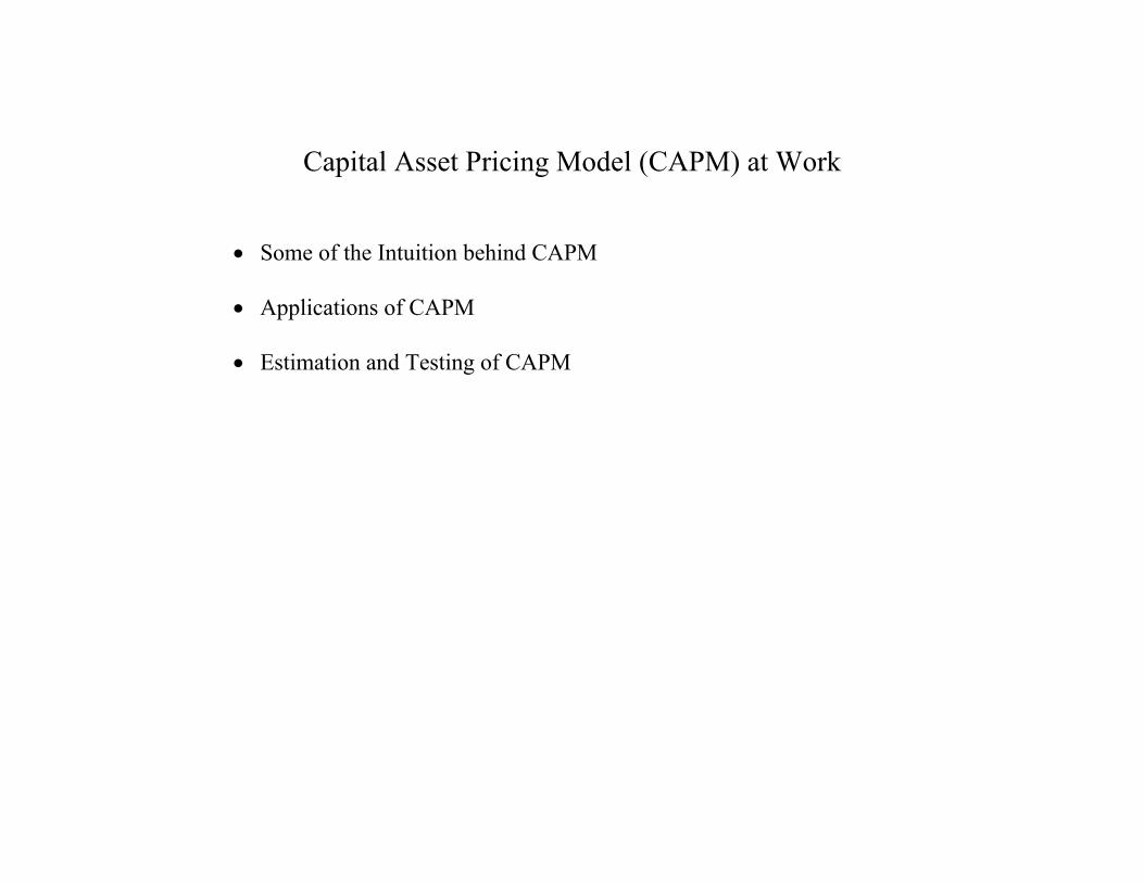
Intuition behind Equilibrium Suppose you observed the following characteristics of two of your stocks within your portfolio (completely ignore risk for now). What do you do?

Stock A Stock B

Current Market Price $100 $50

Expected Selling Price $108 $59 Expected Dividend per

Share $2 $1

Expected (simple) Rate of Return 10% 20%

S S

D D

Stock B

$100

$50

Stock A

S S

D D

Stock B

$100

$50

Stock A

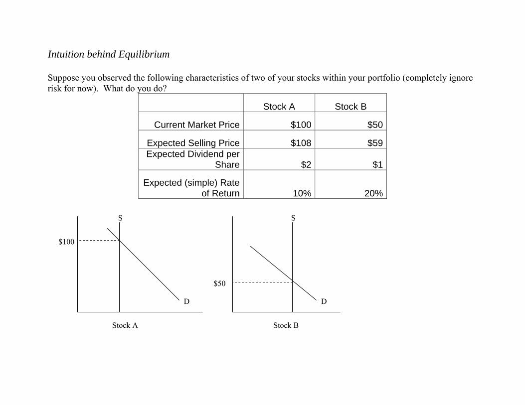
If the price of stock A dropped to $95.65 and stock B rose to $52.17, then what would be the result?

Stock A Stock B

Current Market Price $95.65 $52.17

Expected Selling Price $108 $59 Expected Dividend per

Share $2 $1

Expected (simple) Rate of Return 15% 15%

How would things be different if stock A was more ‘risky’ than stock B? What if stock B was more ‘risky’ than stock A?

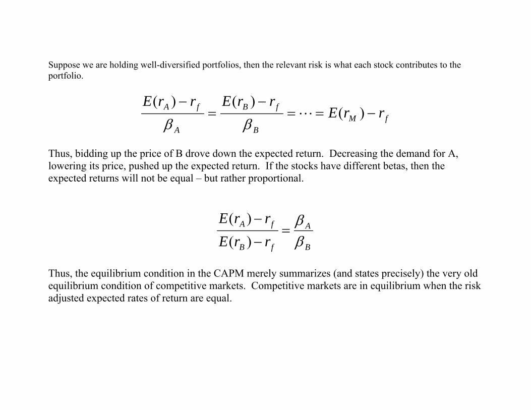
Suppose we are holding well-diversified portfolios, then the relevant risk is what each stock contributes to the portfolio.

fMB

fB

A

fA rrErrErrE

−==−

=−

)()()(

Lββ

Thus, bidding up the price of B drove down the expected return. Decreasing the demand for A, lowering its price, pushed up the expected return. If the stocks have different betas, then the expected returns will not be equal – but rather proportional.

B

A

fB

fA

rrErrE

ββ

=−

−

)()(

Thus, the equilibrium condition in the CAPM merely summarizes (and states precisely) the very old equilibrium condition of competitive markets. Competitive markets are in equilibrium when the risk adjusted expected rates of return are equal.

Applications Assume the expected return on the market to be 15%, risk-free rate of 8%, expected rate of return on XYZ security of 17%, and beta of XYZ security of 1.25. Within the context of CAPM, is XYZ overpriced, underpriced, or fairly priced?

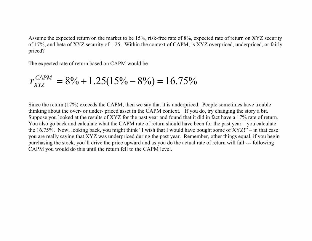
Assume the expected return on the market to be 15%, risk-free rate of 8%, expected rate of return on XYZ security of 17%, and beta of XYZ security of 1.25. Within the context of CAPM, is XYZ overpriced, underpriced, or fairly priced? The expected rate of return based on CAPM would be

%75.16%)8%15(25.1%8 =−+=CAPMXYZr

Since the return (17%) exceeds the CAPM, then we say that it is underpriced. People sometimes have trouble thinking about the over- or under- priced asset in the CAPM context. If you do, try changing the story a bit. Suppose you looked at the results of XYZ for the past year and found that it did in fact have a 17% rate of return. You also go back and calculate what the CAPM rate of return should have been for the past year – you calculate the 16.75%. Now, looking back, you might think “I wish that I would have bought some of XYZ!” – in that case you are really saying that XYZ was underpriced during the past year. Remember, other things equal, if you begin purchasing the stock, you’ll drive the price upward and as you do the actual rate of return will fall --- following CAPM you would do this until the return fell to the CAPM level.

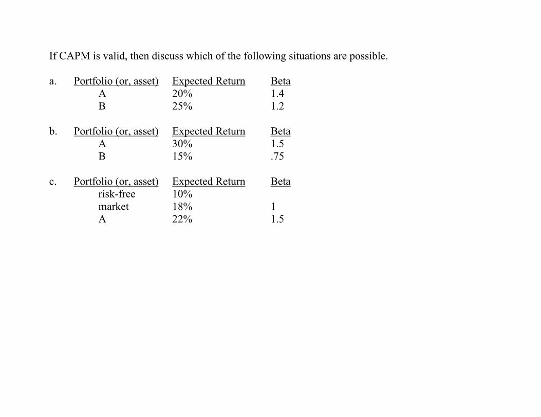
If CAPM is valid, then discuss which of the following situations are possible. a. Portfolio (or, asset) Expected Return Beta A 20% 1.4 B 25% 1.2 b. Portfolio (or, asset) Expected Return Beta A 30% 1.5 B 15% .75 c. Portfolio (or, asset) Expected Return Beta risk-free 10% market 18% 1 A 22% 1.5

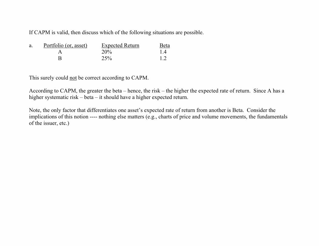
If CAPM is valid, then discuss which of the following situations are possible. a. Portfolio (or, asset) Expected Return Beta A 20% 1.4 B 25% 1.2 This surely could not be correct according to CAPM. According to CAPM, the greater the beta – hence, the risk – the higher the expected rate of return. Since A has a higher systematic risk – beta – it should have a higher expected return. Note, the only factor that differentiates one asset’s expected rate of return from another is Beta. Consider the implications of this notion ---- nothing else matters (e.g., charts of price and volume movements, the fundamentals of the issuer, etc.)

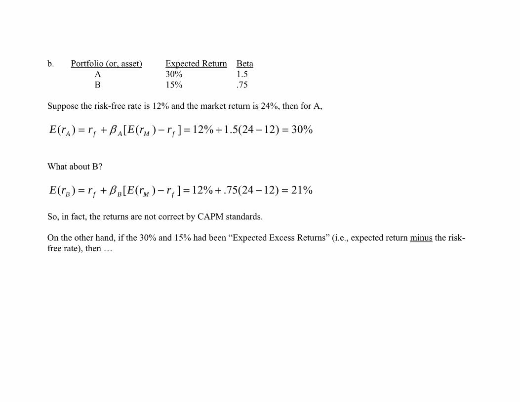
b. Portfolio (or, asset) Expected Return Beta A 30% 1.5 B 15% .75 Suppose the risk-free rate is 12% and the market return is 24%, then for A,

%30)1224(5.1%12])([)( =−+=−+= fMAfA rrErrE β What about B?

%21)1224(75.%12])([)( =−+=−+= fMBfB rrErrE β So, in fact, the returns are not correct by CAPM standards. On the other hand, if the 30% and 15% had been “Expected Excess Returns” (i.e., expected return minus the risk-free rate), then …

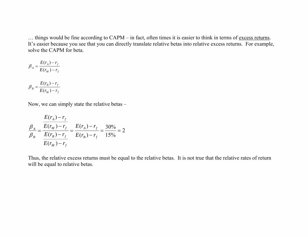
… things would be fine according to CAPM – in fact, often times it is easier to think in terms of excess returns. It’s easier because you see that you can directly translate relative betas into relative excess returns. For example, solve the CAPM for beta.

fM

fAA rrE

rrE−

−=

)()(

β

fM

fBB rrE

rrE−

−=

)()(

β

Now, we can simply state the relative betas –

2%15%30

)()(

)()()()(

==−

−=

−

−−

−

=fB

fA

fM

fB

fM

fA

B

A

rrErrE

rrErrErrErrE

ββ

Thus, the relative excess returns must be equal to the relative betas. It is not true that the relative rates of return will be equal to relative betas.

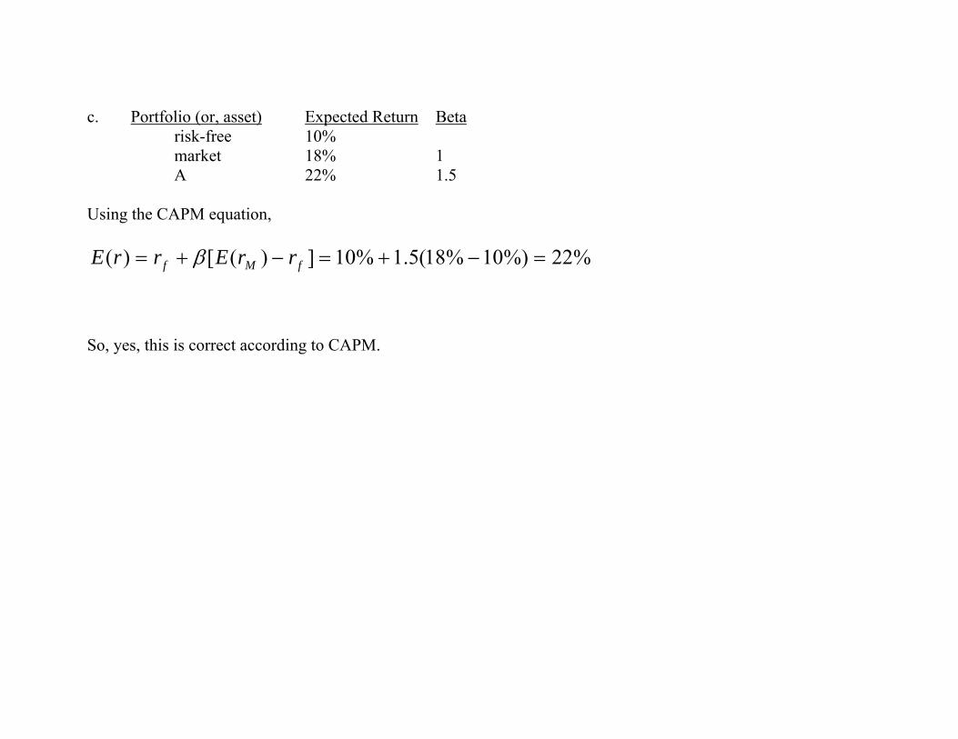
c. Portfolio (or, asset) Expected Return Beta risk-free 10% market 18% 1 A 22% 1.5 Using the CAPM equation,

%22%)10%18(5.1%10])([)( =−+=−+= fMf rrErrE β So, yes, this is correct according to CAPM.

Suppose the equity holders’ (i.e., owners of the stock) investment in the publicly regulate utility company is $100 million and beta is 0.60. If the risk-free rate is 3% and the expected rate of return on the market is 5%, then calculate the ‘fair’ – according to CAPM - rate of return for investors and their profits.

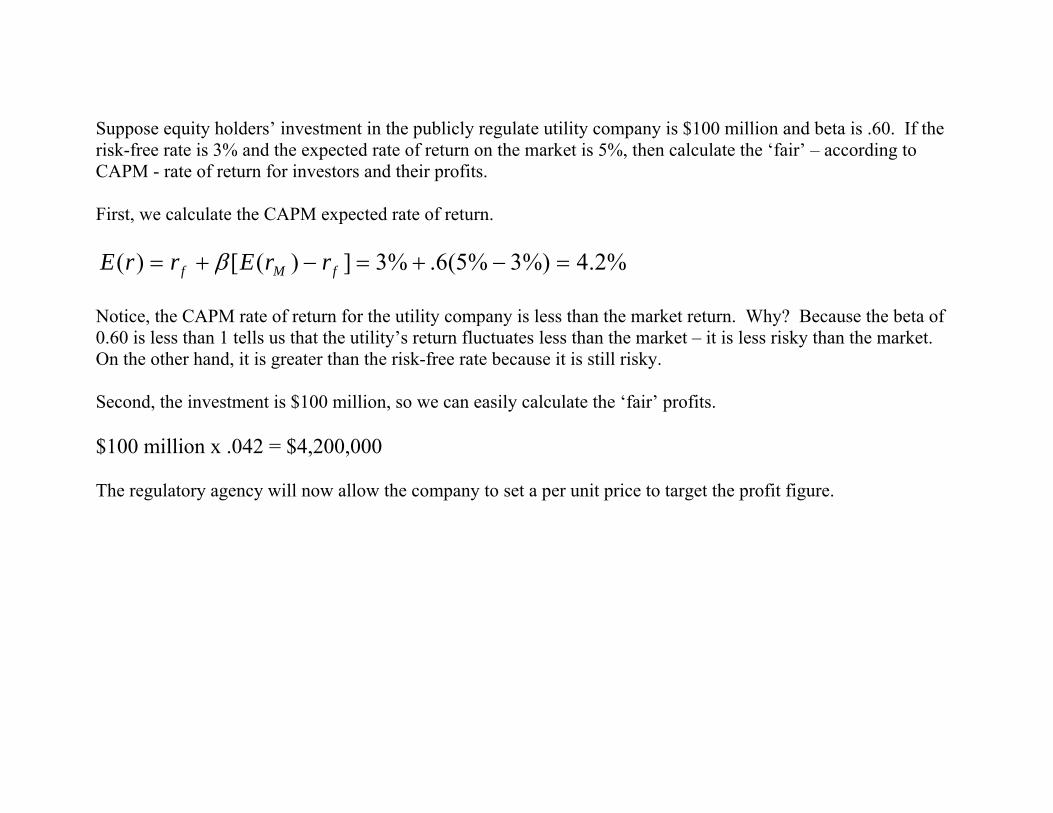
Suppose equity holders’ investment in the publicly regulate utility company is $100 million and beta is .60. If the risk-free rate is 3% and the expected rate of return on the market is 5%, then calculate the ‘fair’ – according to CAPM - rate of return for investors and their profits. First, we calculate the CAPM expected rate of return.

%2.4%)3%5(6.%3])([)( =−+=−+= fMf rrErrE β Notice, the CAPM rate of return for the utility company is less than the market return. Why? Because the beta of 0.60 is less than 1 tells us that the utility’s return fluctuates less than the market – it is less risky than the market. On the other hand, it is greater than the risk-free rate because it is still risky. Second, the investment is $100 million, so we can easily calculate the ‘fair’ profits. $100 million x .042 = $4,200,000 The regulatory agency will now allow the company to set a per unit price to target the profit figure.

A judge uses CAPM to determine the damages in a copyright infringement case. The judge has been advised that a beta of 2.0 is typical for the publishing industry. What would be the ‘fair’ – according to CAPM - rate of return to be used to determine damages? [assume a market return of 14% and risk-free rate of 4%]

A judge uses CAPM to determine the damages in a copyright infringement case. The judge has been advised that the a beta of 2.0 is typical for the publishing industry. What would be the ‘fair’ – according to CAPM - rate of return to be used to determine damages? [assume a market return of 14% and risk-free rate of 4%]

%24%)4%14(2%4)( =−+=rE

The owner of an investment firm is deciding on whether or not to pay a bonus to his two portfolio managers. One manager (Mr. Marko) was able to obtain a 22% rate of return on his portfolio – the portfolio had a beta of 1.5. The other manager (Mr. Witz) was able to earn a 12% rate of return on his portfolio – the portfolio had a beta of 1.0. Assuming the owner uses a CAPM criteria to determine bonuses, which manager - if any – deserves the bonus? [assume a market return of 14% and risk-free rate of 4%]

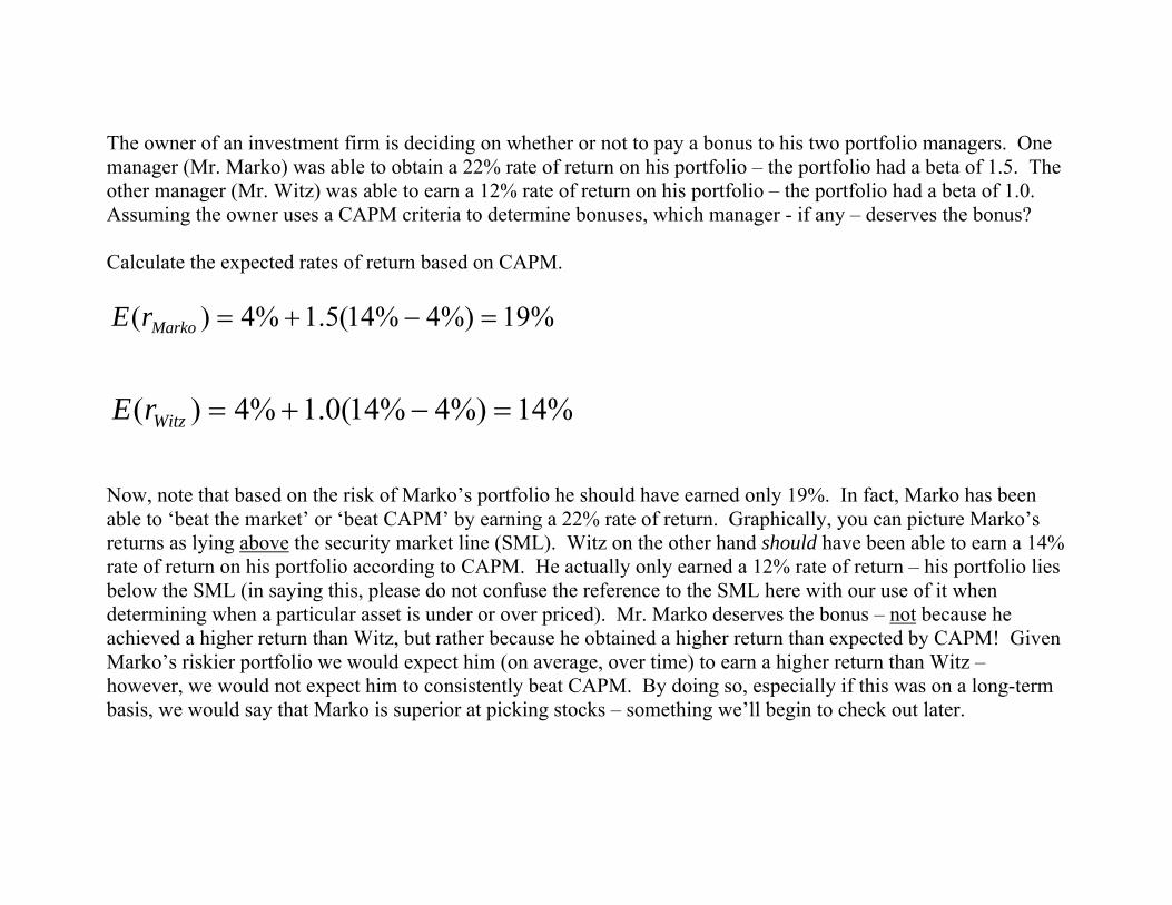
The owner of an investment firm is deciding on whether or not to pay a bonus to his two portfolio managers. One manager (Mr. Marko) was able to obtain a 22% rate of return on his portfolio – the portfolio had a beta of 1.5. The other manager (Mr. Witz) was able to earn a 12% rate of return on his portfolio – the portfolio had a beta of 1.0. Assuming the owner uses a CAPM criteria to determine bonuses, which manager - if any – deserves the bonus? Calculate the expected rates of return based on CAPM.

%19%)4%14(5.1%4)( =−+=MarkorE

%14%)4%14(0.1%4)( =−+=WitzrE Now, note that based on the risk of Marko’s portfolio he should have earned only 19%. In fact, Marko has been able to ‘beat the market’ or ‘beat CAPM’ by earning a 22% rate of return. Graphically, you can picture Marko’s returns as lying above the security market line (SML). Witz on the other hand should have been able to earn a 14% rate of return on his portfolio according to CAPM. He actually only earned a 12% rate of return – his portfolio lies below the SML (in saying this, please do not confuse the reference to the SML here with our use of it when determining when a particular asset is under or over priced). Mr. Marko deserves the bonus – not because he achieved a higher return than Witz, but rather because he obtained a higher return than expected by CAPM! Given Marko’s riskier portfolio we would expect him (on average, over time) to earn a higher return than Witz – however, we would not expect him to consistently beat CAPM. By doing so, especially if this was on a long-term basis, we would say that Marko is superior at picking stocks – something we’ll begin to check out later.

An entrepreneur is considering purchasing a business. The entrepreneur expects the business to have yearly profits – forever – of $1 million. The risk-free rate is currently 8% and the expected rate of return on the market is 18%. The entrepreneur believes that the beta for this business is 1.15. How much should the entrepreneur pay for this business?

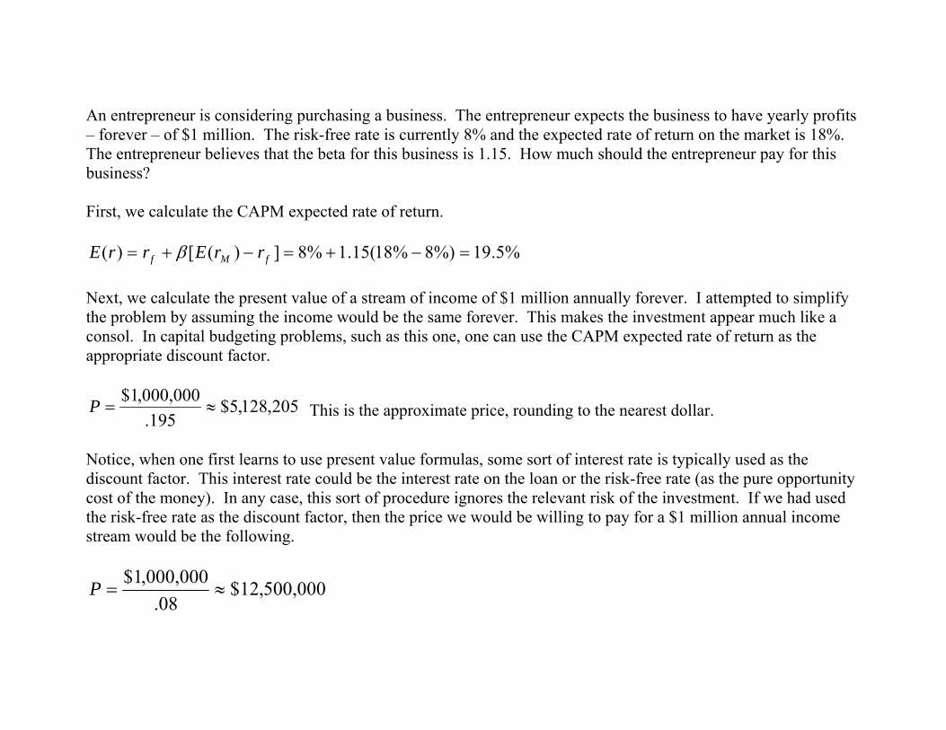
An entrepreneur is considering purchasing a business. The entrepreneur expects the business to have yearly profits – forever – of $1 million. The risk-free rate is currently 8% and the expected rate of return on the market is 18%. The entrepreneur believes that the beta for this business is 1.15. How much should the entrepreneur pay for this business? First, we calculate the CAPM expected rate of return.

%5.19%)8%18(15.1%8])([)( =−+=−+= fMf rrErrE β Next, we calculate the present value of a stream of income of $1 million annually forever. I attempted to simplify the problem by assuming the income would be the same forever. This makes the investment appear much like a consol. In capital budgeting problems, such as this one, one can use the CAPM expected rate of return as the appropriate discount factor.

205,128,5$195.

000,000,1$≈=P This is the approximate price, rounding to the nearest dollar.

Notice, when one first learns to use present value formulas, some sort of interest rate is typically used as the discount factor. This interest rate could be the interest rate on the loan or the risk-free rate (as the pure opportunity cost of the money). In any case, this sort of procedure ignores the relevant risk of the investment. If we had used the risk-free rate as the discount factor, then the price we would be willing to pay for a $1 million annual income stream would be the following.

000,500,12$08.

000,000,1$≈=P

Estimation & Testing of CAPM

])([)( fMf rrErrE −+= β What are some of the difficulties in estimating CAPM?

• History vs. Expectations?

• Time Frame?

• What is the “market”?

• What is the risk-free rate? {for any students that will ever be in a situation of using the CAPM, please note that there exists more than one definition of beta (e.g., levered vs. unlevered betas) and many ways to estimate a beta}

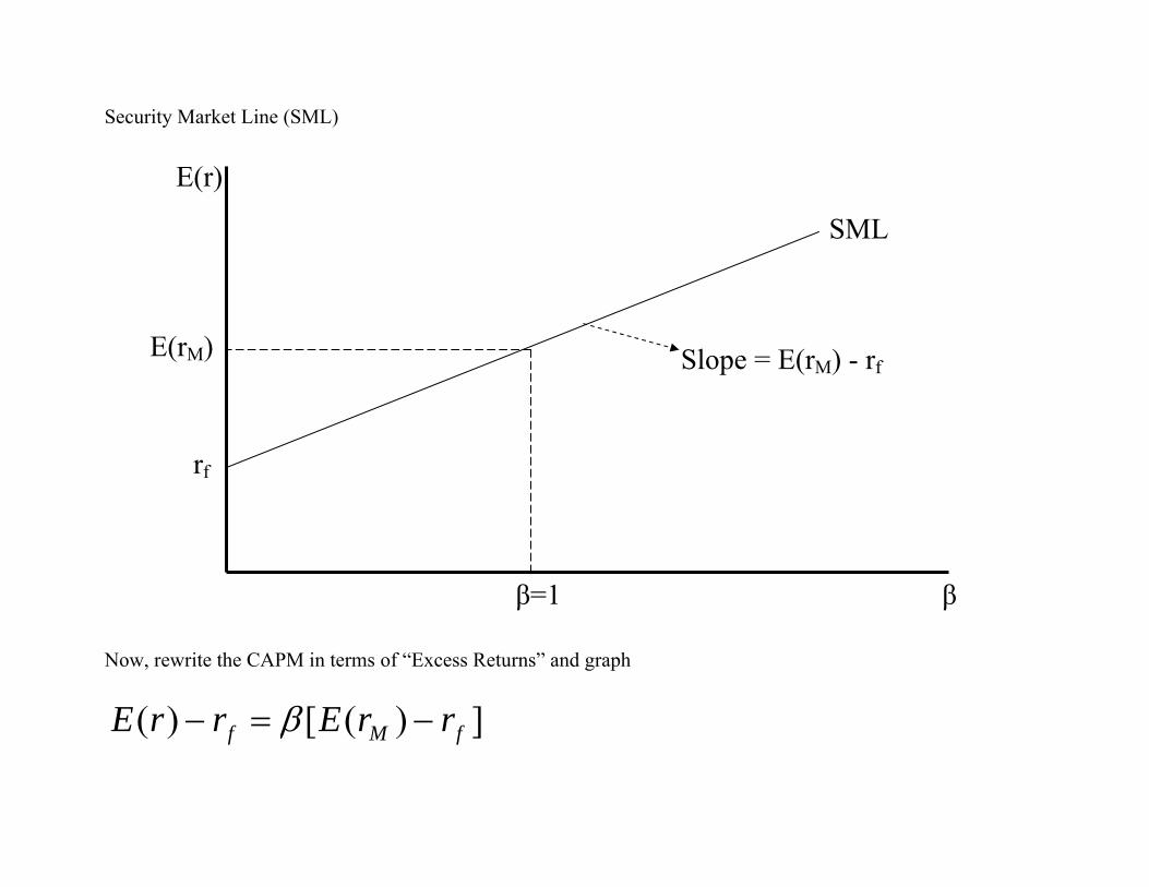
Security Market Line (SML)

rf

E(r)

β

SML

Slope = E(rM) - rf

β=1

E(rM)

Now, rewrite the CAPM in terms of “Excess Returns” and graph

])([)( fMf rrErrE −=− β

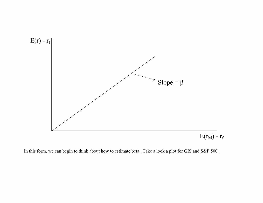
Slope = β

E(rM) - rf

E(r) - rf

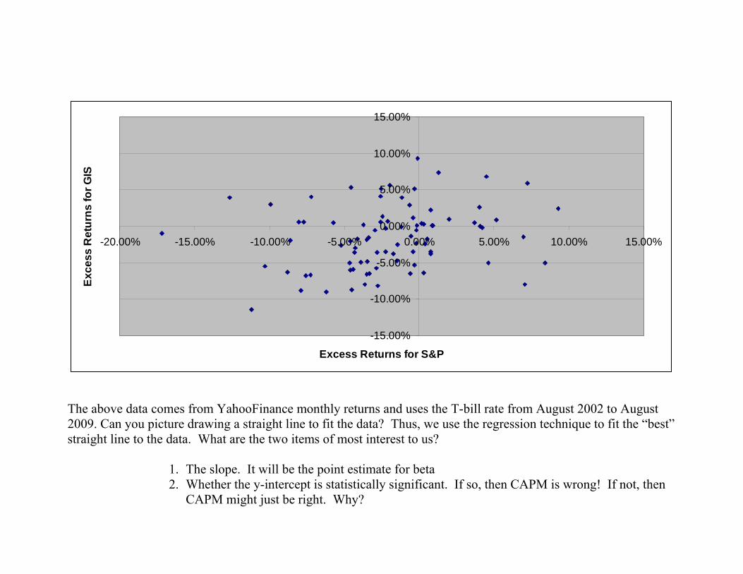
In this form, we can begin to think about how to estimate beta. Take a look a plot for GIS and S&P 500.

-15.00%

-10.00%

-5.00%

0.00%

5.00%

10.00%

15.00%

-20.00% -15.00% -10.00% -5.00% 0.00% 5.00% 10.00% 15.00%

Excess Returns for S&P

Exce

ss R

etur

ns fo

r GIS

The above data comes from YahooFinance monthly returns and uses the T-bill rate from August 2002 to August 2009. Can you picture drawing a straight line to fit the data? Thus, we use the regression technique to fit the “best” straight line to the data. What are the two items of most interest to us?

1. The slope. It will be the point estimate for beta 2. Whether the y-intercept is statistically significant. If so, then CAPM is wrong! If not, then

CAPM might just be right. Why?

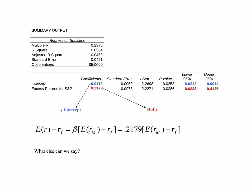
SUMMARY OUTPUT

Regression Statistics Multiple R 0.2375 R Square 0.0564 Adjusted R Square 0.0450 Standard Error 0.0421 Observations 85.0000

Coefficients Standard Error t Stat P-value Lower 95%

Upper 95%

Intercept -0.0113 0.0050 -2.2698 0.0258 -0.0212 -0.0014Excess Returns for S&P 0.2179 0.0978 2.2271 0.0286 0.0233 0.4125

y-intercept Beta

])([2179.])([)( fMfMf rrErrErrE −=−=− β

What else can we say?

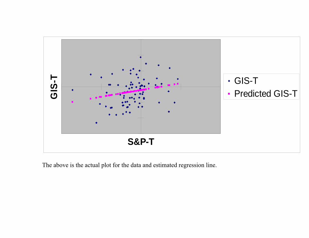
S&P-T

GIS

-T GIS-TPredicted GIS-T

The above is the actual plot for the data and estimated regression line.

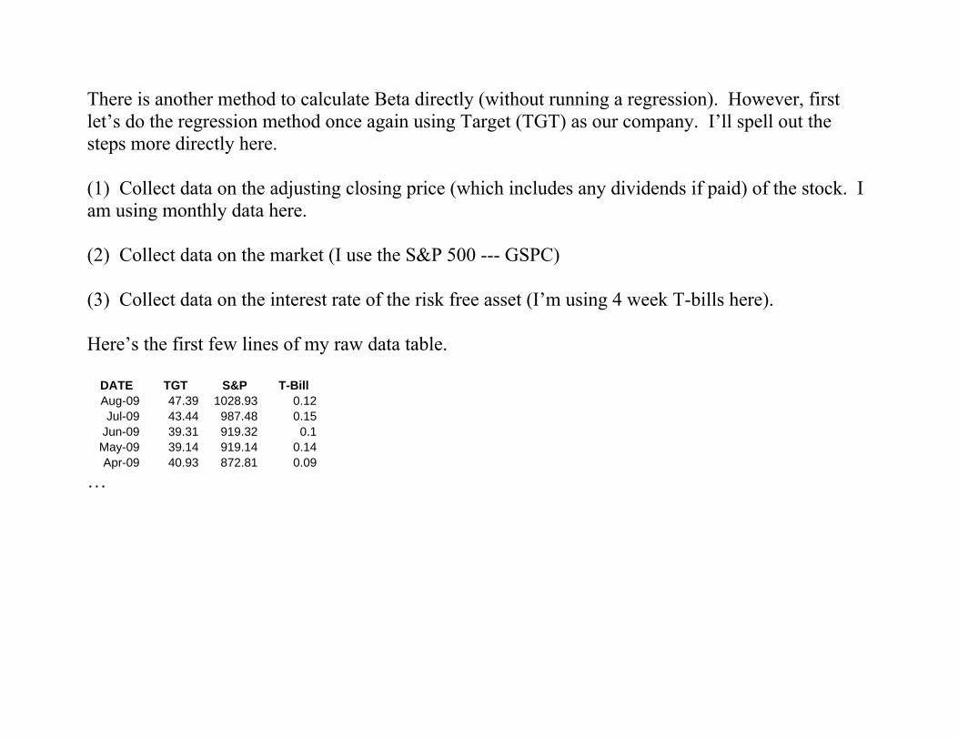
There is another method to calculate Beta directly (without running a regression). However, first let’s do the regression method once again using Target (TGT) as our company. I’ll spell out the steps more directly here. (1) Collect data on the adjusting closing price (which includes any dividends if paid) of the stock. I am using monthly data here. (2) Collect data on the market (I use the S&P 500 --- GSPC) (3) Collect data on the interest rate of the risk free asset (I’m using 4 week T-bills here). Here’s the first few lines of my raw data table.

DATE TGT S&P T-Bill Aug-09 47.39 1028.93 0.12Jul-09 43.44 987.48 0.15

Jun-09 39.31 919.32 0.1May-09 39.14 919.14 0.14Apr-09 40.93 872.81 0.09

…

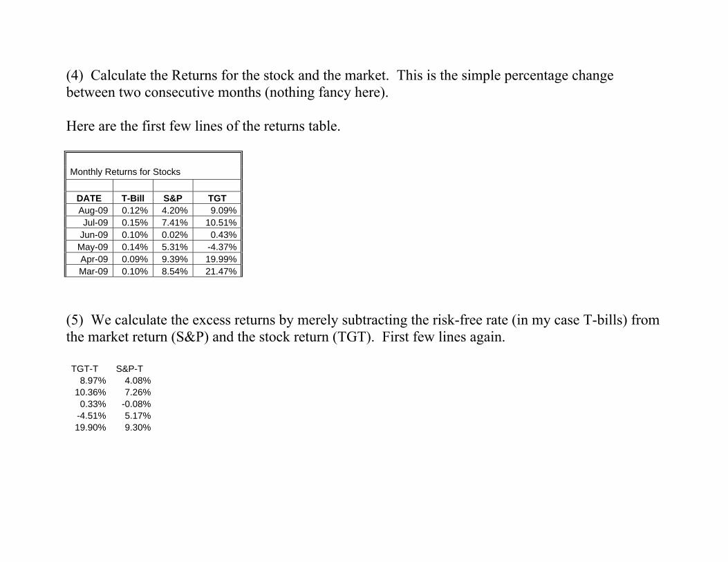
(4) Calculate the Returns for the stock and the market. This is the simple percentage change between two consecutive months (nothing fancy here). Here are the first few lines of the returns table.

Monthly Returns for Stocks

DATE T-Bill S&P TGT Aug-09 0.12% 4.20% 9.09%Jul-09 0.15% 7.41% 10.51%

Jun-09 0.10% 0.02% 0.43%May-09 0.14% 5.31% -4.37%Apr-09 0.09% 9.39% 19.99%Mar-09 0.10% 8.54% 21.47%

(5) We calculate the excess returns by merely subtracting the risk-free rate (in my case T-bills) from the market return (S&P) and the stock return (TGT). First few lines again. TGT-T S&P-T

8.97% 4.08% 10.36% 7.26%

0.33% -0.08% -4.51% 5.17% 19.90% 9.30%

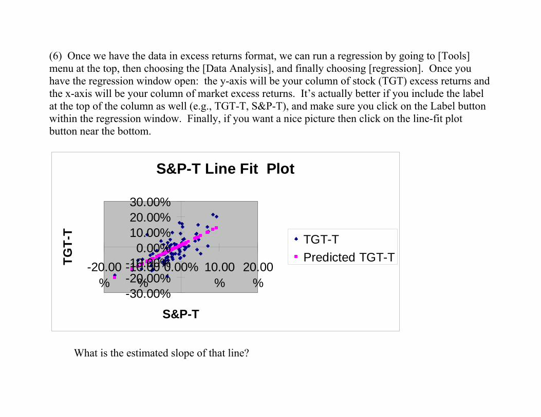
(6) Once we have the data in excess returns format, we can run a regression by going to [Tools] menu at the top, then choosing the [Data Analysis], and finally choosing [regression]. Once you have the regression window open: the y-axis will be your column of stock (TGT) excess returns and the x-axis will be your column of market excess returns. It’s actually better if you include the label at the top of the column as well (e.g., TGT-T, S&P-T), and make sure you click on the Label button within the regression window. Finally, if you want a nice picture then click on the line-fit plot button near the bottom.

S&P-T Line Fit Plot

-30.00%-20.00%-10.00%

0.00%10.00%20.00%30.00%

-20.00%

-10.00%

0.00% 10.00%

20.00%

S&P-T

TGT-

T TGT-TPredicted TGT-T

What is the estimated slope of that line?

SUMMARY OUTPUT

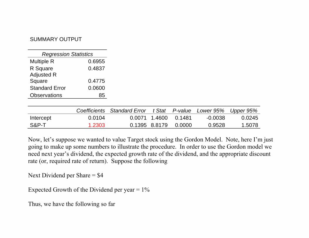
Regression Statistics Multiple R 0.6955 R Square 0.4837 Adjusted R Square 0.4775 Standard Error 0.0600 Observations 85

Coefficients Standard Error t Stat P-value Lower 95% Upper 95%Intercept 0.0104 0.0071 1.4600 0.1481 -0.0038 0.0245S&P-T 1.2303 0.1395 8.8179 0.0000 0.9528 1.5078

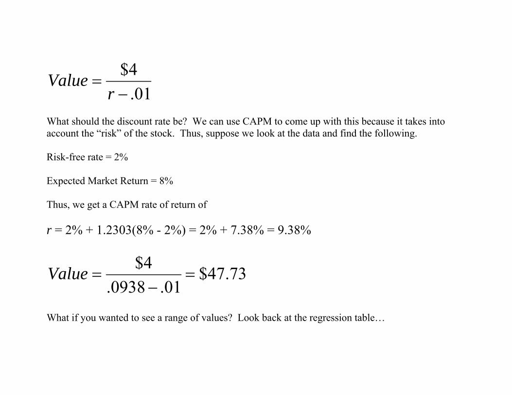
Now, let’s suppose we wanted to value Target stock using the Gordon Model. Note, here I’m just going to make up some numbers to illustrate the procedure. In order to use the Gordon model we need next year’s dividend, the expected growth rate of the dividend, and the appropriate discount rate (or, required rate of return). Suppose the following Next Dividend per Share = $4 Expected Growth of the Dividend per year = 1% Thus, we have the following so far

01.4$

−=

rValue

What should the discount rate be? We can use CAPM to come up with this because it takes into account the “risk” of the stock. Thus, suppose we look at the data and find the following. Risk-free rate = 2% Expected Market Return = 8% Thus, we get a CAPM rate of return of r = 2% + 1.2303(8% - 2%) = 2% + 7.38% = 9.38%

73.47$01.0938.

4$=

−=Value

What if you wanted to see a range of values? Look back at the regression table…

SUMMARY OUTPUT

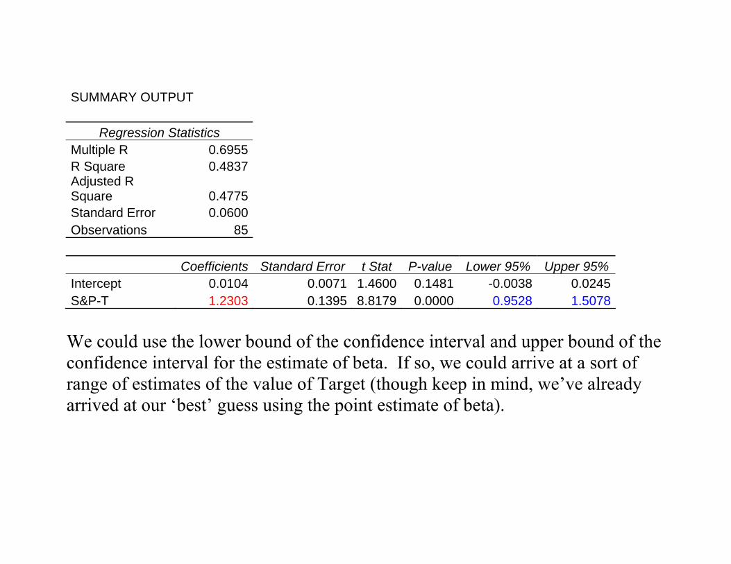
Regression Statistics Multiple R 0.6955 R Square 0.4837 Adjusted R Square 0.4775 Standard Error 0.0600 Observations 85

Coefficients Standard Error t Stat P-value Lower 95% Upper 95%Intercept 0.0104 0.0071 1.4600 0.1481 -0.0038 0.0245S&P-T 1.2303 0.1395 8.8179 0.0000 0.9528 1.5078 We could use the lower bound of the confidence interval and upper bound of the confidence interval for the estimate of beta. If so, we could arrive at a sort of range of estimates of the value of Target (though keep in mind, we’ve already arrived at our ‘best’ guess using the point estimate of beta).

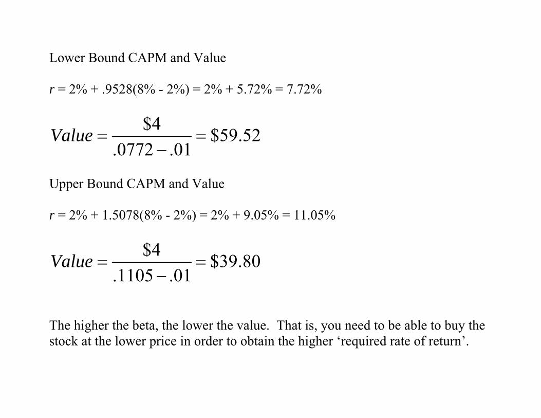
Lower Bound CAPM and Value r = 2% + .9528(8% - 2%) = 2% + 5.72% = 7.72%

52.59$01.0772.

4$=

−=Value

Upper Bound CAPM and Value r = 2% + 1.5078(8% - 2%) = 2% + 9.05% = 11.05%

80.39$01.1105.

4$=

−=Value

The higher the beta, the lower the value. That is, you need to be able to buy the stock at the lower price in order to obtain the higher ‘required rate of return’.

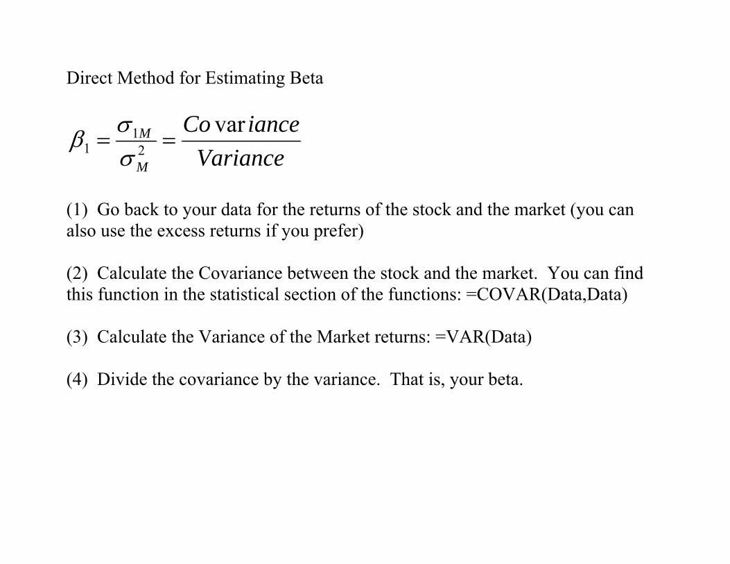
Direct Method for Estimating Beta

VarianceianceCo

M

M var2

11 ==

σσβ

(1) Go back to your data for the returns of the stock and the market (you can also use the excess returns if you prefer) (2) Calculate the Covariance between the stock and the market. You can find this function in the statistical section of the functions: =COVAR(Data,Data) (3) Calculate the Variance of the Market returns: =VAR(Data) (4) Divide the covariance by the variance. That is, your beta.