Some neural network applications in environmental …...Some neural network applications in environmental sciences output parameter xi as a continuous function of multiple input variables

359

Some neural network applications

in environmental sciences: Advancing computational

efficiency of environmental numerical models

Vladimir M. Krasnopolsky1 and

Frederic Chevallier

Research Department

1National Centers for Environmental Prediction, USA Submitted to Neural Networks

November 2001

For additional copies please contact The Library ECMWF Shinfield Park Reading, Berks RG2 9AX [email protected] Series: ECMWF Technical Memoranda A full list of ECMWF Publications can be found on our web site under: http://www.ecmwf.int/pressroom/publications.html © Copyright 2001 European Centre for Medium Range Weather Forecasts Shinfield Park, Reading, Berkshire RG2 9AX, England Literary and scientific copyrights belong to ECMWF and are reserved in all countries. This publication is not to be reprinted or translated in whole or in part without the written permission of the Director. Appropriate non-commercial use will normally be granted under the condition that reference is made to ECMWF. The information within this publication is given in good faith and considered to be true, but ECMWF accepts no liability for error, omission and for loss or damage arising from its use.

http://www.ecmwf.int/pressroom/publications.html

Some neural network applications in environmental sciences

Abstract A new generic neural network (NN) application -- improving computational efficiency of certain processes in numerical environmental models – is considered. This approach can be used to accelerate the calculations and improve the accuracy of the parameterizations of several types of physical processes which generally require computations involving complex mathematical expressions, including differential and integral equations, rules, restrictions and highly nonlinear empirical relations based on physical or statistical models. It is shown that, from a mathematical point of view, such parameterizations can usually be considered as continuous mappings (continuous dependencies between two vectors) and, therefore, NNs can be used to replace primary parameterization algorithms. In addition to fast and accurate approximation of the primary parameterization, NN also provides the entire Jacobian for very little computation cost. Four particular real-life applications of the NN approach are presented here: for oceanic numerical models, a NN approximation of the UNESCO equation of state of the sea water (NN for the density of the seawater) and an inversion of this equation (NN for the salinity of the seawater); for atmospheric numerical models, a NN approximation for long wave radiative transfer code; and for wave models, a NN approximation for the nonlinear wave-wave interaction. In all considered applications a significant acceleration of numerical computations has been achieved. The first two of these NN applications have already been implemented in the operational multi scale ocean forecast system at NCEP. The NN approach introduced in this paper can provide numerically efficient solutions to a wide range of problems in numerical models where lengthy, complicated calculations, which describe physical, chemical and/or biological processes, must be repeated frequently. Keywords: neural networks, numerical modeling, atmospheric modeling, oceanic modeling, wave modeling, equation of state, nonlinear interaction, parameterization of physics

1. Introduction

In this paper, we discuss a recently emerged application of neural networks for efficient (fast and accurate) calculations of the computationally expensive and complex mathematical formulations involved in environmental numerical models, like forecast systems. Any atmospheric or oceanic circulation model is based on a set of prognostic and diagnostic differential equations together with additional equations required to obtain a mathematically closed system. Such a system, in principle, can then be solved to predict the evolution of the environment in time if the initial conditions and any required external boundary conditions are prescribed. Even though the forecast problem may now be considered solvable in a theoretical sense, in the real world of simulation, it is necessary to deal with practical aspects of available computational resources and minimize the computer time taken to produce a run, in particular in the context of operational forecast systems.

The numerical model contains coefficients that appear in the dynamical equations, such as turbulence coefficients representing the unresolvable subgrid scale processes, which need to be parameterized in terms of the dependent variables. Also, implicitly contained in the system are processes that deal with model physics such as radiation, convection, nonlinear wave-wave interaction, etc, which need to be parameterized. Accurate treatments of such parameterizations generally require computations involving complex mathematical expressions, which may include differential and integral equations, rules, restrictions, highly nonlinear empirical expressions, etc. that are developed based on physical or statistical models. The complex mathematical formulations of these processes require considerable computational resource.

Technical Memorandum No. 359 1


For example, a spectral atmospheric model with a well-developed description of physics and subgrid scale parameterizations may spend up to 70% of calculation time for simulating these processes (Estrade et al. 2000). The long wave radiative code requires more than 10% of the computing time in the European Centre for Medium-Range Weather Forecast (ECMWF) general circulation model and in the National Centers for Environmental Prediction (NCEP) global model, even though the computations are not afforded at every grid point (at ECMWF) and at every time step.

In ocean models the estimation of the full UNESCO equation of state to compute the seawater density, represented by an empirically derived highly nonlinear equation relating density to pressure, salinity, and temperature, takes a very significant amount (~40%) of the total computational effort. In addition, most forecast models include data assimilation procedures as an integral part of the forecast system to improve the initial conditions of the model. When dealing with ocean models, most often the data assimilation consists of assimilating surface and subsurface temperature observations to correct the model’s thermal field. This temperature correction automatically makes it necessary to adjust the salinity field in the ocean model in order to avoid gravitational instabilities in the water column. This requires inverting the complicated oceanic equation of state, which makes the computational effort even more time-consuming than the forward problem of computing the density itself. Another example where intensive computational is needed in a forecast model is the calculation of the land surface temperature using a set of equations describing the atmospheric boundary layer and physical processes in the soil. Yet another example of intensive computational problem in forecast models is the wind wave forecasting problem in which an exact calculation of the nonlinear wave-wave interactions using the formulation of Hasselmann (1963) takes a prohibitively long time.

In view of the constraints imposed on the available computer resources, the calculation time allowed for each parameterization is strictly limited in most operational forecast models. Hence, very often it is found necessary to use simplified forms of these complex representations in carrying out the time integrations in a forecast model, thereby sacrificing accuracy of forecasts to a certain extent. For example, the nonlinear wave interactions in a wave forecast model are replaced by a simplified discrete interaction approximation (DIA) (see Hasselmann et al 1985). Similarly, simplified fast parameterizations of physics are used in many parts of atmospheric and oceanic models. In most of these cases, accurate physical models have been developed, but they cannot be used because they are too expensive computationally. Often simplified (even oversimplified due to computational efficiency requirements) parameterizations are obtained, for example, by neglecting higher order terms of perturbation theory, by using empirical approximations, or simply by neglecting the effects, which complicate the calculations. It is common in many parameterization schemes that the number of input and output variables is relatively small, whereas the volume of internal calculations is large. A typical example is the parameterization of the radiative fluxes in the atmosphere. Indeed accurate treatment of cloud-radiation and aerosol-radiation interactions involves elaborate and numerically onerous 3-dimensional scattering methods. Hence, most often the specific parameterization is a result of a compromise between accuracy and computational efficiency with an (sometimes) unpredictable effect on the forecast.

Improvements in forecast modeling can be achieved not only by improving the representation of such parameterizations as our understanding of the underlying physical processes increases but also by improving

2 Technical Memorandum No. 359


our ability to compute these parameterizations accurately within the constraints imposed by the available computer resources.

In this paper we present some of the problems dealing with physical parameterizations and their computations from a different (formal mathematical) point of view, namely that of improving the computational efficiency of available algorithms. We propose a generic approach, which is based on developing fast and accurate parameterizations of physics by approximating solutions of exact physical models using neural networks (NNs). From this formal point of view an exact (best known) physical model representing a physical process performs a smooth conversion of an input vector of parameters,

1 2, ..., , nnX x x x X= ∈ ℜ into an output vector of parameters, 1 2, ..., , m

ny y Y=Y y .Thus, each

output parameter yi is a continuous function of multiple input variables x1, x2, ..., xn (input vector X). Symbolically this input-output dependence is depicted in Fig. 1.a and can be written as

∈ ℜ

m∈ ℜ (1.a) ( ); ,nY F X X Y= ∈ ℜ

Y = F(X)

y1

y3

y2

y4

ym

F f

x1

x2

x3

x4

xn

X = f(Y)

x1

x2

x3

x4

xn

a. b.

Figure 1. Graphical representation of forward (a) and inverse (b) parameterizations

If X and Y are related through a cause and effect principle, the forward parameterization, eq. (1.a), can be derived from first principles. If the inverse dependence

(1.b) ( ); ,nX f Y X Y= ∈ ℜ ∈ Mℜ

is required (see Fig. 1.b) in a numerical model, the inverse problem should be solved, which implies that eq. (1.a) should be inverted. A solution of the inverse problem (1.b) or an inverse parameterization provides each



output parameter xi as a continuous function of multiple input variables y1, y2, ..., yn (vector Y is an input vector now). Forward, eq. (1.a), and inverse, eq. (1.b), parameterizations represent the same mathematical object - a continuous mapping which is a continuous relationship between two vectors. Usually these input/output relationships are highly complex and nonlinear, but continuous, for physical processes taken into account in atmospheric, oceanic, and wave models. Hence, if exact solutions to these complex relationships are calculated, however expensive the computational efforts may be, these solutions can be used by the generic mathematical tool - that is, the NNs - to produce fast and accurate approximations for continuous mappings (Funahashi 1989, Cybenko 1989, Chen and Chen 1995a,b, Attali J-G. and G. Pagès 1997). In this approach the costly exact calculation of the physics needs to be performed only once and “off line” to enable the development of the fast and accurate approximation. After that only this fast and accurate approximation will be used to calculate the physics (coefficients of differential equations) “on line” in a numerical model.

We assume that the readers of this journal are well familiar with the NN technique. Therefore we do not describe this technique in the paper. We only present here a brief list of main properties of NNs, which make them a very suitable generic tool for our application.

• NNs are able to accurately approximate complicated nonlinear input/output relationships (any continuous nonlinear mapping).

• while training the NN is often time consuming, its application is not. After the training is finished (it is usually performed only once), each application of the trained NN is an estimation of a simple algebraic expression with known coefficients, which is practically instantaneous (several tens of floating point additions and multiplications).

• NNs are analytically differentiable, in a way that make the calculation of entire Jacobian matrix cheap.

• NN technique is flexible enough to accommodate various additional constraints, which may arise in this application.

In Section 2 of this paper we present two (forward and inverse) parameterizations for oceanic models, in Section 3 for atmospheric, and in Section 4 a parameterization for wind wave models developed using NNs. In Section 5, we discuss some important features of our approach and some generalizations of standard NN techniques, which are required to accommodate these features.

2. Oceanic Applications: Neural Networks for Efficient Calculation of Sea Water Density or Salinity from the UNESCO Equation of State


In this section, we apply a NN technique to two related problems in the fast calculation of physics in oceanic modeling and data assimilation. (i) In most ocean models, the UNESCO International Equation of State for Seawater (e.g., UNESCO, 1981) (UES) is used for the calculation of the seawater density at each point of a 3-D grid using a relatively small time step. The frequency of updating the density depends on specifics of the model. For high-resolution models, the solution of this equation consumes a significant part of the overall computation time. (ii) In the data assimilation process, assimilation of temperature alone, without making


corresponding adjustments to salinity, in ocean models, which employ the full equation of state, can lead to problems of gravitational instabilities (Woodgate 1998, Chalikov et al. 1998). To adjust the salinity, we need to calculate the salinity from UES as a function of temperature, density and depth (or pressure), i.e. solve an inverse problem in many points. Numerical inversion of the UES is an iterative procedure, which can consume several orders of magnitude more time than solving of the UES itself.

The UES for seawater gives the following expression for the density anomaly δρ (kg/m3) as described by Foffonoff and Millard (1983),

( ), , ( , , ) 1000T S P T S Pρδ ρ= −

( , ,0)( , , )

1( , , )

T ST S P PK T S P

ρρ =−

(2)

where ρ is the density of seawater in kg/m3, T is the temperature in °C, S is the salinity in practical salinity units (psu), P is the pressure, and K(T, S, P) is a bulk modulus.

The UES (2) is empirically based and given over a three-dimensional domain D = -2 < T < 40°C, 0 < S < 40 psu, and 0 < P < 10000 decibars. This domain represents all possible combinations of T, S, and P, which are globally encountered. Mathematically, the functions ρ(T, S, 0) and K(T, S, P) are represented by multidimensional high degree polynomials and, as a result, the density (2) is a ratio of two three-dimensional polynomials which contain more than 40 parameters.

The UES has two major drawbacks when it is applied in the context of ocean modelling. The first is its cumbersome form. For high-resolution models, the solution of this equation at each point of a three-dimensional grid for each time step consumes a significant part (up to 40%) of the overall computation time. Second, it is not a simple matter using the UES to obtain solutions for salinity, since this solution represents an inverse dependence.

The UES determines the density field from observed temperature, salinity, and pressure to within a standard error of approximately 0.009 kg m-3; however, there are several natural processes (e.g. variations in the composition of dissolved salts) (Apel, 1987), contributing to the uncertainty in the density of natural seawater. The resulting natural uncertainty in the density is of the order of 0.1 kg m-3 (Krasnopolsky et al. 2000, 2001b). Taking these uncertainties into account, it does not make sense to use parameterization with higher accuracy in numerical ocean models if accuracy and computing time grow up together. This is why the accuracy of about 0.1 kg m-3 was selected as the expected accuracy for the NN parameterization. The accuracy of the NN parameterization for salinity expressed in terms of density was also expected to be of about 0.1 kg m-3.

Since the depth Z is used in NCEP ocean model as a vertical coordinate, and there exist a simple pressure-depth relationship (Krasnopolsky et al. 2001b), we use Z instead of P in our consideration. The UES defines two relationships (second relationship for salinity through inversion),



( , , )T S Zρ ρ= (3.a)

( , , )S S T Zρ= (3.a)

which are continuous mappings (degenerated mappings because one dimensional vectors are on the left). The NN technique can be applied to approximate any continuous mappings (Funahashi 1989, Cybenko 1989, Chen and Chen 1995a,b). To create a training set for these NN parameterizations in the three-dimensional domain D (see above), 4,000 points (Ti,Si,Zi) were generated on a grid. The UES was used to estimate the density of seawater, ρi, for each point. This simulated data set ρi,Ti, Si, Zi was used in order to train the NNs to extract density and salinity. NNs with three nonlinear neurons in one hidden layer and one linear neuron in the output layers were selected. Two NN parameterizations were obtained (see also Fig. 2):

( , , )NN T S Zρ ρ= (4.a)

( , , )NNS S T Zρ= (4.a)

where both ρNN and SNN are expressed by :

(5) ( ) ( ) ( ) ( )

1 1( ) tanh

k nS S S

NN j ji i jj i

S xρ ρ ρρ ω= =

= Ω +

∑ ∑i SB ρβ+

T

ρ (S)

S ( ρ ) Z

∂ρ ∂ ( )ST

∂ρ ∂ ρ

( ) ( ) S

S

Fig 2 Schematic representation of NN parameterizations for the density and salinity of seawater. Additional outputs for derivatives are not trained, they are calculated.

Derivatives (Jacobian matrix) shown in Fig. 2 as additional NN outputs are not actual outputs, which are trained during the NN training; they are calculated analytically through direct differentiating eq. (5). The NN parameterization (4a) for the density is about two times faster then the UES. The calculation of the Jacobian



matrix with the NN parameterization requires an additional time, which is about 70% of time required for the calculation of density. The NN parameterization (4b) for the salinity is several hundreds times faster than an iterative numerical inversion of the UES; the time required for the numerical inversion of the UES (rate of conversion of the iteration process) varies significantly. It strongly depends on inversion algorithm and on the choice of the initial approximation for the salinity.

To evaluate the accuracy of the NN approximation (4), 16,000 points were generated within the domain D on a grid, which did not include the training set points. The density of sea water calculated from the UES (2) was compared to that calculated from the NN, ( , , )NN T S Zρ , using (4.a). Table 1 shows several statistical

measures of the differences (or errors) between the UES and the NN estimates for density. In terms of the bias and the RMS differences, the NN results for density clearly satisfy the criterion mentioned above; both the bias and the RMS values do not exceed the uncertainties indicated there and are less than 0.1 kg m-3.

Min ε Max ε Bias RMS

-0.12 0.15 0.00 0.04

Table 1. Minimum, maximum, and mean (i.e., the bias) errors (ε) and the RMS error,

all expressed in kg m-3 ( )UES NNε ρ ρ= −

To evaluate the errors in using the NN approach to estimate the salinity, we used the same 16,000 points ( , , , )i i i iT S Zρ which were used for estimating the density. Initially, the NN for SNN (4.b) was applied to

calculate a new salinity, si, using the corresponding values ( , , )i i iT Zρ . Then the differences (Si - si) were

utilized to estimate the accuracy of the NN-derived salinities (first line in Table 2). To further evaluate the quality of the NN-derived salinities, the UES was applied again, this time to the triad ( , to

recalculate the density of seawater,

, )i i iT s Z

iρ′ . If the NN-obtained values for salinity were perfect, then the density,

iρ′ , would be equal to iρ . The differences between these two values, ( iρ - iρ′ ), were then used to further

estimate the accuracy of the salinity-trained NN in terms of the density (second line in Table 2).

Units Min error Max error Mean error RMS error

PSU -0.33 0.85 0.00 0.10

Kg m-3 -0.27 0.71 0.00 0.08

Table 2. Accuracies of the salinities estimated by the NN in terms of salinity and density. Minimum, maximum, and mean errors together with the RMS errors are presented.

Table 2 shows that the NN estimates of salinity (4.b) have an RMS error of 0.1 psu. In terms of the related error in density, this accuracy corresponds to an RMS error of 0.08 kg m-3, which again does not exceed the uncertainties discussed above.



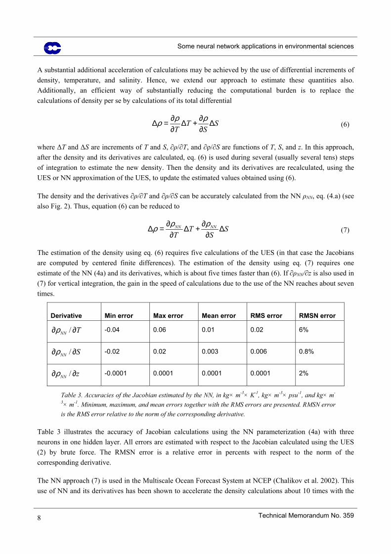
A substantial additional acceleration of calculations may be achieved by the use of differential increments of density, temperature, and salinity. Hence, we extend our approach to estimate these quantities also. Additionally, an efficient way of substantially reducing the computational burden is to replace the calculations of density per se by calculations of its total differential

TT S

Sρ ρρ ∂ ∂∆ = ∆ + ∆∂ ∂

(6)

where ∆T and ∆S are increments of T and S, ∂ρ/∂T, and ∂ρ/∂S are functions of T, S, and z. In this approach, after the density and its derivatives are calculated, eq. (6) is used during several (usually several tens) steps of integration to estimate the new density. Then the density and its derivatives are recalculated, using the UES or NN approximation of the UES, to update the estimated values obtained using (6).

The density and the derivatives ∂ρ/∂T and ∂ρ/∂S can be accurately calculated from the NN ρNN, eq. (4.a) (see also Fig. 2). Thus, equation (6) can be reduced to

NN NNTT S

Sρ ρρ ∂ ∂∆ = ∆ + ∆∂ ∂

(7)

The estimation of the density using eq. (6) requires five calculations of the UES (in that case the Jacobians are computed by centered finite differences). The estimation of the density using eq. (7) requires one estimate of the NN (4a) and its derivatives, which is about five times faster than (6). If ∂ρNN/∂z is also used in (7) for vertical integration, the gain in the speed of calculations due to the use of the NN reaches about seven times.

Derivative Min error Max error Mean error RMS error RMSN error

/NN Tρ∂ ∂ -0.04 0.06 0.01 0.02 6%

/NN Sρ∂ ∂ -0.02 0.02 0.003 0.006 0.8%

/NN zρ∂ ∂ -0.0001 0.0001 0.0001 0.0001 2%

Table 3. Accuracies of the Jacobian estimated by the NN, in kg× m-3× K-1, kg× m-3× psu-1, and kg× m-

3× m-1. Minimum, maximum, and mean errors together with the RMS errors are presented. RMSN error is the RMS error relative to the norm of the corresponding derivative.

Table 3 illustrates the accuracy of Jacobian calculations using the NN parameterization (4a) with three neurons in one hidden layer. All errors are estimated with respect to the Jacobian calculated using the UES (2) by brute force. The RMSN error is a relative error in percents with respect to the norm of the corresponding derivative.

The NN approach (7) is used in the Multiscale Ocean Forecast System at NCEP (Chalikov et al. 2002). This use of NN and its derivatives has been shown to accelerate the density calculations about 10 times with the



error in the density calculations not exceeding the natural uncertainty 0.1 kg/m3. Therefore, the computational expense of calculating density has decreased from 40% to about 4-5% of the total time of integration as a result of using the NN approximation in the model.

3. Atmospheric Applications: Neural Networks for Efficient Calculation of Infrared Radiative Fluxes

The next application that we present tackles the problematic tradeoff between accuracy and rapidity in the atmospheric infrared radiation computations. Transfer of energy by infrared radiation significantly contributes to the variations of atmospheric temperature. Now, the infrared atmospheric spectrum encompasses a wide range of variability, from the slow-varying Planck function to the very detailed structures of the individual absorption bands. As a consequence, accurate modeling of the atmospheric radiative processes requires a high spectral resolution, which consumes a lot of computing time, and therefore can hardly be used for simulation of the atmosphere. Radiation computations also involve integrals over solid angle and altitude, that cannot be analytically solved and therefore significantly add to the computational burden. Two strategies are used, often simultaneously, to make the models affordable. On the one hand, statistical approaches have been developed that simplify the calculations of the three integrals (over solid angle, altitude and wave number) and of the impact of clouds (Goody and Yung 1989). On the other hand the computations are not performed at every time step and at every grid point of the atmospheric model (Morcrette 2000). As an example, in the NCEP forecast model, infrared radiation variables are updated every three hours only.

The computational efficiency is even more an issue in elaborate four-dimensional variational (4D-Var) analysis schemes. These powerful data assimilation systems have been developed in operational weather centers, like ECMWF or MétéoFrance, to correct the atmospheric forecasts at regular times with the observations that have been received since the previous analysis: 4D-Var determines a statistically optimum forecast, given the initial forecast and its assumed error characteristics on the one side, and the observations with their error specifications on the other (e.g., Courtier et al. 1994). To do this, perturbations of the atmosphere need to be propagated in time at every step of the minimization process with a linearized physics. Only computationally very cheap parameterizations can be used for this purpose. For instance, in the operational 4D-Var physics at ECMWF, radiation perturbations are created by temperature changes only. Neither water vapor nor cloud evolution is taken into account (Mahfouf 1999).

Neural network-based radiative transfer models (e.g., Escobar-Munoz et al. 1993, Key and Schweiger 1998, Faure et al. 2001, Schwander et al. 2001) may be able to address these issues. In particular, the NeuroFlux approach (Chéruy et al. 1996, Chevallier et al. 1998b) has been successively tested in the Laboratoire de Météorologie Dynamique climate model (Chevallier et al. 1998a), in the ECMWF forecast model (Chevallier et al. 2000b) and is currently being tested in the ECMWF 4D-Var system. This section describes the method, updates the results and summarizes the experience gained by this approach on which a lot of effort has been invested.

NeuroFlux is mainly a neural-network-based version of the broadband radiation model of Morcrette (1991), hereafter EC-OPE, even though other models could be used in the training. EC-OPE was the operational



code at ECMWF in the 90s. The integration over wave number is performed using a band emissivity method in six spectral regions covering the long-wave spectrum. The transmission functions for water vapor and carbon dioxide are fitted using Padé approximants. Multi-layer gray bodies represent the clouds (Washington and Williamson, 1977).

NeuroFlux has been derived from EC-OPE using the same cloud representation and the Multi-Layer Perceptron. Consistently with the former, upward and downward fluxes are computed in NeuroFlux as:

(8) ( ) ( ) ( )i k i kk

F P a P F P=∑ i i

where Pi is the pressure level, Fk is the infrared flux in the presence of a single layered black cloud in atmospheric layer k or the clear-sky flux (with the convention k=0 for clear sky), and ak is a weight. The ak’s are computed with a simple parameterization as a function of the layered cloud characteristics (cloud cover, liquid and ice water contents, particle size, etc…) and depend on the way cloudy layers overlap. In NeuroFlux, the Fk’s are computed with artificial neural networks with single hidden layers, whereas EC-OPE uses the above-mentioned band-emissivity method.

To summarize, NeuroFlux is made of a battery of specialized NNs (one for each atmospheric layer k and for each type of flux -upward or downward-), the inputs of which include the temperature and gas (water vapor and ozone) profiles, the surface characteristics and the mean carbon dioxide concentration, whereas the cloud characteristics are processed by a separate parameterization. This way of doing reduces the dimension of the individual NNs, compared to a system where all computations would be performed by a single NN.

With that design, NeuroFlux is about eight times faster than EC-OPE.

The accuracy of NeuroFlux has been assessed through code-by-code comparisons, climate simulations, and 10-day forecasts. Figure 3 and 4 illustrate the performance of the version that fits the 50-level vertical resolution that was used in the ECMWF operational forecast system in 1999. The accuracy of NeuroFlux is comparable to the accuracy of EC-OPE, with a neutral impact on the simulations. In particular the uncertainty introduced by NeuroFlux in the cloud cover simulations was shown to be much smaller than that one induced by the reduced temporal frequency of radiation computation in the ECMWF climate simulations (Chevallier et al., 2000b).

Even though the inputs of the NNs in NeuroFlux do not include the cloud profiles, some of the NNs reach sizes that are unusually large. For instance, the NN that compute the clear-sky upward fluxes in a 60-layer vertical grid contains about 200 inputs and 60 outputs. As a consequence of this huge variable space, the set up of the training datasets is particularly involving. It relies on the sampling of hundreds of thousands of atmospheric profiles with a simple topologic approach, as described by Chevallier et al. (2000a). Similar work is done each time the vertical resolution is increased, because new levels are expected to provide original information about the profiles that cannot be obtained by a simple interpolation from the lower resolution datasets. Each version of the training datasets includes more than ten thousand profiles.



Fig 3 Statistics of the differences between the computations of NeuroFlux and those of EC-OPE: cooling rates from NeuroFlux minus cooling rates from EC-OPE. ECMWF 6-hour forecasts, L50 T319 (about 60 km horizontal resolution). 1 February 1999, 00, 06, 12 and 18 UTC. The infrared cooling rates are the contribution of the infrared radiation to the variations of temperature over time. They are proportional to the derivative of the net fluxes with respect to pressure

Fig 4 L50 T319 (about 60 km horizontal resolution) simulations: forecast verification for temperature expressed in terms of mean temperature bias over the Northern Hemisphere (12 cases) The forecast system uses either EC-OPE (full



lines) or NeuroFlux (circles)

Despite the large number of synoptic weights in NeuroFlux, the partial derivatives of the computed fluxes with respect to atmospheric variables (i.e. the Jacobians) contain features that are considered not to be realistic (Chevallier and Mahfouf 2000). In other words, the characteristics of the small noise of the computed fluxes (Figure 3) critically show up in the flux Jacobians. This is different from the behavior of the smaller NNs presented in Section 2 (Table 3). Regularization techniques, such as that one proposed by Aires et al. (1999), only partially improve the quality of the NN computation. Larger NNs may solve the problem, but would complicate the training even more and would slow down the code, making it less attractive. This issue of having correct sensitivities is very important for the application to 4D-Var where first-order Taylor developments of the parameterizations are used. However, the approach of NeuroFlux allows for an elegant solution. Equation (8) is differentiated as:

(9) ( ) ( ) ( ) ( ) ( )i k i k i k i kk

dF P a P dF P F P da P= +∑ i i i

Equation (9) is used to calculate the flux perturbations. Its terms are determined as follows. The ak’s and the Fk’s are obtained from NeuroFlux. A pre-computed mean Jacobian matrix, instead of the unsatisfactory NeuroFlux Jacobians, allows for a reasonably accurate estimation of the dFk’s using a first-order Taylor approximation, since those partial fluxes are weakly non-linear. Finally, the dak’s are obtained analytically from the tangent-linear version of the ak model.

This approach is faster than the full tangent-linear model of NeuroFlux by almost a twofold factor, which makes it even more attractive. It is being evaluated as part of an improved version of the 4D-Var linearized physics at ECMWF, which introduces the treatment of the interaction between cloud and radiation (Janisková et al. 2000). This package includes NeuroFlux, a shortwave radiation model and a diagnostic cloud scheme, on top of the currently-operational simplified and linearized physics. It is evaluated by studying the linearized time evolution of analysis increments with reference to the non-linear computation using the full physics of the forecast model. An improvement (respectively a degradation) of the tangent-linear trajectory makes it closer to (respectively further away from) the non-linear one. A quotation mark, as defined by (Janisková et al. 2000), quantifies this impact for any model variable. Figure 5 illustrates the positive impact of the new physics on the wind increments after a 12-hour integration, with a global improvement of 3.3%. Therefore the tangent-linear wind increments are more realistic when the new physical package is used. Preliminary results show a subsequent improvement of the forecast quality (Janisková, personal communication, 2001).



Fig 5 L60 T159 (about 125 km horizontal resolution). Zonal mean impact of the new linearized physics (with NeuroFlux) on the zonal component of the wind, in m.s-1, in a 12-hour simulation starting on 15 March 2001 00 UTC. Negative (respectively positive) values indicate an improvement (respectively a degradation) compared to the previous linearized physics. Both linearized physics are evaluated with reference to the non-linear run.

4. Wave Application: A Neural Network Approximation for Nonlinear Interactions in Wind Wave Models

Ocean wind wave modeling for hindcast and forecast purposes has been at the centre of interest for many decades. Numerical prediction models are generally based on a form of the spectral energy or action balance equation

in nl ds swDF S S S SDt

= + + + (8)

where F is the spectrum, Sin is the input source term, Snl is the nonlinear interaction source term, Sds is the dissipation or ‘whitecapping’ source term, and Ssw represents additional shallow water source terms. The JONSWAP study (Hasselman et al 1973) identified the active role of the nonlinear interactions in wave growth. The SWAMP study (SWAMP Group 1985) then identified the need for explicit modeling of Snl in wave models. State-of-the-art or so-called third generation wave models therefore explicitly model this source term.

In its full form (e.g., Hasselmann and Hasselmann 1985), the calculation of the interactions Snl requires the integration of a six-dimensional Bolzmann integral:



( )4 4 1 2 3 4 1 2 3 4 1 2 3 4

1 3 4 2 2 4 3 1 1 2 3

2

( ) ( ) ( , , , ) ( ) ( )

( )

( )( ) ; tanh( )

nlS k T F k G k k k k k k k k

n n n n n n n n dk dk dk

F kn k g k kh

ω δ δ ω ω

ωω

= ⊗ = ⋅ + − − ⋅ + − −

× ⋅ ⋅ − + ⋅ ⋅ −

= = ⋅ ⋅

∫ ω ω

(9)

where the complicated coupling coefficient G contains moving singularities (K. Hasselmann 1963). This integration requires roughly 103 to 104 times more computational effort than all other aspects of the wave model combined. Present operational constraints require that the computational effort for the estimation of Snl should be of the same order of magnitude as the remainder of the wave model. This requirement was met with the development of the Discrete Interaction Approximation (DIA, Hasselmann et al 1985). The development of the DIA allowed for the successful development of the first third-generation wave model WAM (WAMDI Group 1988, Komen et al. 1994). More than a decade of experience with the WAM model and its derivatives has identified shortcomings of the DIA. The DIA tends to unrealistically increase the directional width of spectra, has a systematic spurious impact on the shape of the spectrum near the spectral peak frequency, and has a much too strong signature at high frequencies. In present third generation wave models, these deficiencies can be countered at least in part by the dissipation source term Sds, which is generally used for tuning the energy balance in the equation (8). Although this approach gives good results, it is counterproductive, because it prohibits development of dissipation source terms based on solid physical considerations. With our increased understanding in the physics of wave generation and dissipation, this becomes an even bigger obstacle impeding further development of third-generation wave models.

Considering the above, it is of crucial importance for the development of third generation wave models to develop an economical yet accurate approximation for Snl. Here, we explore a Neural Network Interaction Approximation (NNIA) to achieve this goal (see also Krasnopolsky et al 2001a,b). NNs can be applied here because the nonlinear interaction (9) is essentially a nonlinear mapping (symbolically represented in eq. (9) by T) which relates two vectors (2-D fields in this case). Thus, the nonlinear interaction source term can be considered as a nonlinear mapping between a spectrum F and a source term Snl

(10) ( )nlS T F=

where T is the exact nonlinear operator given by the full Bolzmann interaction integral (9) (Hasselmann and Hasselmann 1985, Resio and Perrie 1991). Discretization of S and F (as is necessary in any numerical approach) reduces (10) to continuous mapping of two vectors of finite dimensions. Modern high resolution wind wave models use descretization on a two dimensional grid which leads to dimensions of S and F vectors of order of N > 600 (Tolman 1999). It seems unreasonable to develop a NN approximation of such a high dimensionality (more than 600 inputs and outputs). Moreover, such a NN will be grid dependent.

In order to reduce the dimensionality of the NN and convert the mapping (10) to a continuous mapping of two finite vectors independent on the actual spectral discretization, the spectrum F and source function Snl are expanded using systems of two-dimensional functions each of which (Φi and Ψq) creates a complete and orthogonal two-dimensional basis



1 1

,n m

i i nl q qi q

F x S y ψ= =

≈ Φ ≈∑ ∑ (11)

where for xi and yq we have

,i i q nlx F y S= Φ = Ψq∫∫ ∫∫ (12)

where the double integral identifies integration over the spectral space. Because both sets of basis functions Φii=1,…,n and Ψqq=1,…,m are complete, increasing n and m in (11) improves the accuracy of approximation, and any spectrum F and source function Snl can be approximated by (11) with a required accuracy. Substituting (11) into Eq. (10) we can get

(13) ( )Y T X=

which represents a continuous mapping of the finite vectors and Y , and where T still represents the full nonlinear interaction operator. This operator can be approximated with a NN with n inputs and m outputs and k neurons in the hidden layer

nX ∈ ℜ m∈ ℜ

(14) ( )NNY T X=

The accuracy of this approximation (TNN) is determined by k, and can generally be improved by increasing k.

To train the NN approximation TNN of T, a training set has to be created that consists of pairs of vectors X and Y. To create this training set, a representative set of spectra Fp has to be generated with corresponding (exact) interactions Snl,p using eq. (9). For each pair (F, Snl)p, the corresponding vectors (X,Y)p are determined using eq. (12). These pairs of vectors are then used to train the NN to obtain TNN.

After TNN has been obtained by training, the resulting NN Interaction Approximation (NNIA) algorithm consists of three steps: (1) decompose the input spectrum, F, by applying Eq. (12) to calculate X; (2) estimate Y from X using Eq. (14); and compose the output source function, Snl, from Y using Eq. (11).

A graphical representation of the NNIA algorithm is shown in Figure 6.

The above describes the general procedure for developing an NNIA. Development of an actual NNIA requires the following steps: (1) select basis functions Φi and Ψq and the number of each (n,m); (2) design a NN topology (number of neurons k); (3) construct a representative training set; and (4) select training strategies.

The first three points all have a significant impact on both accuracy and economy of a NNIA. Unfortunately, there is no pre-defined way to tackle these issues as mentioned in section 2. It is therefore unavoidable that the development of a NNIA involves much iteration. The first requirement for a NNIA to be potentially useful in operational wave modeling is that the exact interactions Snl are closely reproduced for



computational costs comparable to that of the DIA. The following shows the potential of this approach with the design of a simple ad-hoc NNIA.

x d f df F f fi i=∞

−∫∫ θ θ θ

π

π

( , ) ( , )0

Φ

y b a xq q q qj ji i j qi

M

j

K

= + + +==∑∑tanh [tanh( )] ω βΩ Β

11

S f y fnl qq

M

q( , ) ( , )θ θ≈=∑

1Ψ

NN

Y

X

F f( , )θ

S fnl ( , )θ

Fig 6 Graphical representation of the NNIA algorithm.

To address the basic feasibility of a NNIA, we have considered a NNIA to estimate the nonlinear interactions Snl(f,θ) as a function of frequency f and direction θ from the corresponding spectrum F(f,θ). Here we present the major results of this study for illustrating our approach (for more details see Krasnopolsky et al. 2001a). To train and test this NNIA, we used a set of about 20,000 simulated realistic spectra for F(f,θ), and the corresponding exact estimates of Snl(f,θ) (Van Vledder et al 2000). Comparison of simulated spectra with spectra generated by the WAVEWATCH model (Tolman 1999, Tolman and Chalikov 1996) shows that approach, which we use for simulating spectra, allowed us to simulate reasonably realistic and complicated spectra describing a broad range of wave systems. Separate data sets have been generated for training and validation.

As is common in parametric spectral descriptions, we choose separable basis functions where frequency and angular dependence are separated. For Φi this implies:



, ,( , ) ( ) ( )i ij f if f θθ jφ φ θΦ ⇒ Φ = (15)

A similar separation is used for Ψq. Considering the strongly suppressed behavior of F and Snl for f → 0, and the exponentially decreasing asymptotic behavior for f → ∞, generalized Laguerre’s polynomials (Abramowitz and Stegun 1964) are used to define φf and ψf. Considering that no directional preferences exist in F and Snl, Fourier decomposition is used for φθ and ψθ. The number of base functions is chosen to be n = 51 and m = 64 to keep the accuracy of approximation for F on average better than 2% and for Snl - better than 5-6%. The number of hidden neurons was k = 30, which allows a satisfactory NN approximation of the mapping (13) using (14).

Mean RMSE σRMSE Max RMSE

DIA 0.0133 0.0111 0.104

NNIA 0.0068 0.0063 0.065

Table 5. RMSE statistics for 10,000 Snl

Table 5 compares three important statistics for the source function RMS errors (with respect to exact solution) calculated using DIA and NNIA for 10,000 spectra (independent validation set). The NNIA is nearly twice as accurate as DIA.

Fig 7 RMSE as functions of frequency f and angle (averaged over entire test set). Dashed line - error of approximation (lower bound for all other errors). Solid line - DIA, line with squares - NNIA (n=51:k=20:m=64), and line with triangles - NNIA (51:30:64)

Figure 7 shows mean RMSE as functions of the frequency f (left) and the angle θ (right). It also illustrates the improvement of the NNIA accuracy by increasing the number of neurons, k, in the hidden layer from 20 to 30. Numbers in Table 5 correspond to a NNIA with 30 neurons in the hidden layer (51:30:64).

And finally, Figure 8 compares the DIA, NNIA, and exact algorithms in terms of the accuracy and computational efficiency. Computational time (in sec) corresponds to a control calculation performed on the



same computer. The current preliminary version of the NNIA algorithm is twice as accurate and only about 5 times slower than the DIA algorithm. In the current version of the wind wave models, an algorithm that is up to 20 times slower than DIA can be accommodated; therefore, we still have enough room for further improving the accuracy of the NNIA. Considering that no optimization has yet been applied in the development of the NNIA composition and decomposition procedures, it appears reasonable to expect a final NNIA algorithm with computation requirements similar to DIA but with significantly better accuracy.

Calculation Time vs. DIA Time

Error vs. DIA Error

1 10 100 1000 10000 100000 10000000

0.5

1

DIA NNIA Exact

Fig 8 Comparison of the accuracy and computational efficiency of the DIA, NNIA, and exact algorithms. The horizontal time scale is logarithmic

5. Summary and discussion

In this paper we presented a recently emerged NN application developed by the authors for simplifying and accelerating time-consuming calculations in environmental numerical models using neural network techniques. Parameterizations of physical, chemical, and biological processes, which occur at different scales, constitute an important class of such calculations. It is shown that, from a mathematical point of view, descriptions of such processes can usually be considered as continuous mappings (continuous dependencies between two vectors). It is known that neural networks are a generic tool for approximation of such mappings and, therefore, can be used for fast and accurate approximation of parameterizations of such processes. NNs can also easily provide analytical Jacobians. Because the NN Jacobian is computationally cheap, this approach is expected to be also very beneficial when used in 3-D and especially in 4-D variational data assimilation systems. We applied this approach to four specific problems associated with oceanic, atmospheric, and wave modeling.



The first and second applications considered in the paper deal with the oceanic equation of state, which is used for estimating the density and salinity of seawater in ocean circulation models. Separate neural networks for density and salinity were developed using the UES as a basis. Although the estimation of density represents a forward problem, estimating salinity from the UES represents a complicated inverse problem, which has been very efficiently solved using the NN approach. The accuracy of the neural network-generated densities and salinities were of the same order as those obtained directly from the UES itself. However, the time required to perform the calculations of density using the neural network and the neural network Jacobian is about ten times less than that for UES. The time required for calculating salinity using the neural network is several hundred times less than that required for the numerical inversion of the USE. Consequently, this approach has direct application to numerical ocean models where the equation of state must be estimated repeatedly. At NCEP, a NN equation for seawater density is currently used in the NCEP oceanic model.

In the third application, the neural network approach was shown to successively handle the parameterization of infrared radiation in atmospheric models and to improve the tradeoff between speed and accuracy of such computation. In particular, the scheme described allows speeding up the computational time by a factor of eight compared to the reference model, while not affecting the quality of the atmosphere simulations. Further improvements of the method include the use of a more accurate reference model in the training phase, such as that currently operational at ECMWF (Morcrette et al. 2001). The high number of variables involved in this NN application made it necessary to develop original approaches, for instance for the set-up of the training dataset. Also, the model computations are split into several modules, each one of them being parameterized by a specific NN. Despite this strategy, the NNs used are still very large, which affects the quality of the Jacobians, because it makes the training more difficult. Further increase of the vertical resolution, or the introduction of additional input or output variables, might further reduce the robustness of the model. This is an obvious limitation in the framework of the forecast models, which complexity constantly increases. However, the approach appears to be suitable for the variational assimilation, where other parts of the physics are very simplified and where the speed factor is crucial. Also, some other aspects of the radiation computation, such as the cloud horizontal heterogeneity, are crudely handled by forecast models and may benefit from NN parameterizations, as illustrated by Faure et al. (2001).

The fourth application deals with the nonlinear wave-wave interactions in wind wave models. A prototype of the NN approximation for this interaction is presented in this work. The NNIA calculations of Snl are about five orders of magnitude faster than the exact parameterization. The NNIA calculations are twice more accurate than those from DIA (oversimplified approximation, which is currently used in the wind wave models) and require only 4-5 times more computational effort than the DIA calculations with less than 5% of this time spent in the actual NN part of the algorithm. Decomposition of the input spectra F and composing the source function Snl from the NN output accounts for the rest. This decomposition (i) significantly reduces the size of the NN and (ii) makes the approach practically independent on the model grid and resolution.

These four applications illustrate the strengths and limits of the NNs for the application to the fast simulation of environmental processes. In the case of retrievals, as discussed by Krasnopolsky (1997) and Krasnopolsky and Schiller (2001), neural networks compete with other statistical methods only, and usually perform better than those because they are able to optimize the statistical link between the inputs and the outputs, provided



that a proper (i.e. diverse and regularly spread) training dataset is gathered. In the present case, a sufficiently accurate physically based direct model is usually available. The neural networks are likely to be faster, but significant speed gains can also be obtained with more powerful computers, making other parameterizations affordable, that were not before. Also, the purely statistical formulation of the neural networks often makes the refinements of their simulations, like additional inputs and outputs, or more complex physics, more difficult than with an explicit physics.

The simulation of environmental processes may involve a large number of inputs (i.e., several hundreds), which make the NN too complex and complicates the training. For this complexity problem, two possible solutions were developed and illustrated: the input and output vectors may be projected on a basis (e.g., the NNIA application) or a battery of smaller NNs may be used (e.g., infrared radiation application).

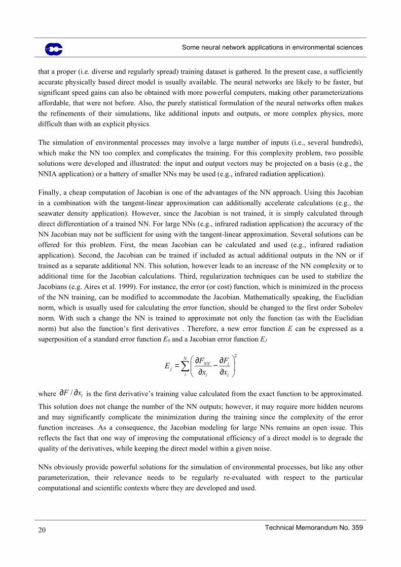
Finally, a cheap computation of Jacobian is one of the advantages of the NN approach. Using this Jacobian in a combination with the tangent-linear approximation can additionally accelerate calculations (e.g., the seawater density application). However, since the Jacobian is not trained, it is simply calculated through direct differentiation of a trained NN. For large NNs (e.g., infrared radiation application) the accuracy of the NN Jacobian may not be sufficient for using with the tangent-linear approximation. Several solutions can be offered for this problem. First, the mean Jacobian can be calculated and used (e.g., infrared radiation application). Second, the Jacobian can be trained if included as actual additional outputs in the NN or if trained as a separate additional NN. This solution, however leads to an increase of the NN complexity or to additional time for the Jacobian calculations. Third, regularization techniques can be used to stabilize the Jacobians (e.g. Aires et al. 1999). For instance, the error (or cost) function, which is minimized in the process of the NN training, can be modified to accommodate the Jacobian. Mathematically speaking, the Euclidian norm, which is usually used for calculating the error function, should be changed to the first order Sobolev norm. With such a change the NN is trained to approximate not only the function (as with the Euclidian norm) but also the function’s first derivatives . Therefore, a new error function E can be expressed as a superposition of a standard error function E0 and a Jacobian error function EJ

2NNN i

ji i i

F FEx x

∂ ∂= − ∂ ∂ ∑

where is the first derivative’s training value calculated from the exact function to be approximated.

This solution does not change the number of the NN outputs; however, it may require more hidden neurons and may significantly complicate the minimization during the training since the complexity of the error function increases. As a consequence, the Jacobian modeling for large NNs remains an open issue. This reflects the fact that one way of improving the computational efficiency of a direct model is to degrade the quality of the derivatives, while keeping the direct model within a given noise.

/ iF x∂ ∂

NNs obviously provide powerful solutions for the simulation of environmental processes, but like any other parameterization, their relevance needs to be regularly re-evaluated with respect to the particular computational and scientific contexts where they are developed and used.



Acknowledgements

We thank M. Janisková, at ECMWF for providing the results of Figure 5. We also thank D. Chalikov, D.B. Rao, and H. Tolman, at NCEP for their help and support in developing oceanic and wave NN applications.

References

Abramowitz, M. and I. A. Stegun, editors (1964) Handbook of Mathematical Functions with Formulas, Graphs and Mathematical Tables, National Bureau of Standards.

Aires, F., M. Schmitt, A. Chédin, and N. A. Scott, 1999: The “weight smoothing” regularization of MLP for Jacobian stabilization. IEEE Trans. Neural Networks, 10, 1502-1510.

Apel, J.R. (1987) Principles of Ocean Physics, Academic Press, New York, p. 145.

Attali J-G. and G. Pagès (1997) Approximations of Functions by a Multilayer Perceptron: A New Approach. Neural Networks, 6, 1069-1081.

Chalikov D., et al. (1998) Revisiting the Question of Assimilating Temperature alone into a Full Equation of State Ocean Model. Ocean Modeling, 116, 13-14.

Chalikov D., D.B. Rao, I. Rivin, V. Krasnopolsky, R. Grumbine (2002) A multi-scale ocean forecast system for applications to global and regional domains. NCEP/NOAA Technical Note, OMB contribution No. 194, Washington DC, 130 pp.

Chen, T. and H. Chen (1995a) Approximation Capability to Functions of Several Variables, Nonlinear Functionals and Operators by Radial Basis Function Neural Networks. Neural Networks, 6, 904-910.

Chen, T. and H. Chen (1995b) Universal Approximation to Nonlinear Operators by Neural Networks with Arbitrary Activation Function and Its Application to Dynamical Systems. Neural Networks, 6, 911-917.

Chéruy, F., F. Chevallier, N. A. Scott and A. Chédin (1996) A fast method using neural networks for computing the vertical distribution of the thermal component of the Earth radiative budget. C. R. Acad. Sci. Paris, t. 322, S. IIb, pp.665-672. [in French]

Chevallier, F., F. Chéruy, Z. X. Li, and N. A. Scott (1998a) A fast and accurate neural network-based computation of longwave radiative budget application in a GCM. Proc. of the Am. Meteor. Soc. Conference, Paris, France, 25-29 May 1998, 690-693.

Chevallier, F., F. Chéruy, N. A. Scott, and A. Chédin (1998b) A neural network approach for a fast and accurate computation of longwave radiative budget. J. Appl. Meteor., 37, 1385-1397.

Chevallier, F., A. Chédin, F. Chéruy, and J.-J. Morcrette (2000a) TIGR-like atmospheric profile databases for accurate radiative flux computation. Q.J. Roy.Meteor.Soc., 126, 761-776.

Chevallier, F., J.-J. Morcrette, F. Chéruy, and N. A. Scott (2000b) Use of a neural-network-based longwave radiative transfer scheme in the EMCWF atmospheric model. Q.J. Roy.Meteor.Soc, 126, 761-776.

Chevallier, F., and J.-F. Mahfouf (2001) Evaluation of the Jacobians of infrared radiation models for variational data assimilation. J. Appl.Meteor., 40, 1445-1461.



Courtier, P., J.-N. Thépaut, A. Hollingsworth (1994) A strategy, for operational implementation of 4D-Var, using an incremental approach. Q. J. Roy. Meteor. Soc., 120, 1367-1388.

Cybenko, G. (1989) Approximation by Superposition of Sigmoidal Functions. Mathematics of Control, Signals and Systems, 2, 303-314.

Escobar-Munoz, J., A. Chédin, F. Chéruy, and N. A. Scott (1993) Réseaux de neurones multi-couches pour la restitution de variables thermodynamiques atmosphériques à l’aide de sondeurs verticaux satellitaires. C. R. Acad. Sci. Paris, 317, 911-918 [in French].

Estrade, J.-F., Y. Trémolet, and J. Sela (2001) Experiments with NCEP’s Spectral Model. In “Developments in Teracomputing - Proceedings of the Ninth ECMWF Workshop on the Use of High Performance Computing in Meteorology, Reading, UK, 13-17 November 2000”, W. Zwieflhofer and N. Kreitz (eds), World Scientific Publishing Co, 92-99.

Faure, T., Isaka, H., Guillemet, B. (2001) Mapping neural network computation of high-resolution radiant fluxes of inhomogeneous clouds. J. Geophys. Res., D106, 14,961-14,974.

Fofonoff, N.P., and R.C. Millard Jr. (1983) Algorithms for computation of fundamental properties of seawater. UNESCO technical paper in marine science 44, UNESCO.

Funahashi, K. (1989) On the Approximate Realization of Continuous Mappings by Neural Networks. Neural Networks, 2, 183-192.

Goody, R. M., and Y. L. Yung (1989) Atmospheric Radiation. Oxford University Press, 519 pp.

Hasselmann, K. (1963) On the non-linear energy transfer in a gravity-wave spectrum. Part 3: Evaluation of the energy flux and swell-sea interaction for a Neumann spectrum. J. Fluid Mech., 15, 385-399.

Hasselmann, K. et al. (1973) Measurements of wind-wave growth and swell decay during the Joint North Sea Wave Project (JONSWAP). Ergänzungshelf zur Deutschen Hydrographischen Zeitschrift, Reihe A (8) Nr.12, 95 pp.

Hasselmann, S. and K. Hasselmann (1985) Computations and parametrizations of the nonlinear energy transfer in a gravity wave spectrum. Part I: a new method for efficient computations of the exact nonlinear transfer integral. J. Phys. Ocean., 15, 1369-1377.

Hasselmann, S. et al. (1985) Computations and parametrizations of the nonlinear energy transfer in a gravity wave spectrum. Part II: parametrization of the nonlinear transfer for application in wave models. J. Phys. Ocean, 15, 1378-91.

Janiskova, M., J.-F. Mahfouf, J.-J. Morcrette, and F. Chevallier (2000) Development of linearized radiation and cloud schemes for the assimilation of cloud properties. ECMWF Technical Memorandum No. 301, 31 pp.

Key, J., and A. J. Schweiger (1998) Tools for atmospheric radiative transfer: Streamer and Fluxnet. Computer and Geosciences, 24, 443-451

Komen, G.J. et al. (1994) Dynamics and Modelling of Ocean Waves, Cambridge University press, Cambridge, 532 pp.



Krasnopolsky V.M. (1997) Neural networks for standard and variational satellite retrievals, NCEP/NOAA Technical Note, OMB contribution No. 148, Washington DC, 43 pp.

Krasnopolsky V.M., et al. (2000) Application of neural networks for efficient calculation of sea water density or salinity from the UNESCO equation of state, Proceedings, Second Conference on Artificial Intelligence, AMS, Long Beach, CA, 9-14 January, 2000, 27-30.

Krasnopolsky V., D.V. Chalikov, and H.L. Tolman (2001a) Using neural network for parameterization of nonlinear interactions in wind wave models, International Joint Conference on Neural Networks, July 15-19, 2001, Washington, DC, 1421-1425

Krasnopolsky V., D.V. Chalikov, and H.L. Tolman (2001b) A neural network technique to improve computational efficiency of numerical oceanic models, Ocean Modelling, to be published

Krasnopolsky V.M. and H. Schiller (2001), Some neural network applications in environmental sciences. Part I: Forward and inverse problems in satellite remote sensing, Neural Networks, submitted.

Mahfouf, J.-F. (1999) Influence of physical processes on the tangent-linear approximation. Tellus, 51A, 147-166.

Morcrette, J.-J. (1991) Radiation and cloud radiative properties in the ECMWF operational weather forecast model. J. Geophys.Res., 96D, 9121-9132.

Morcrette, J.-J. (2000) On the effects of the temporal and spatial sampling of radiation fields on the ECMWF forecasts and analyses. M.Wea.Rev., 128, 876-887.

Morcrette, J.-J. E. J. Mlawer, M. J. Iacono, and S. A. Clough (2001) Impact of the radiation-transfer scheme RRTM in the ECMWF forecasting system. ECMWF Newsletter, No.91, 2-9.

Resio, D.T. and W. Perrie (1991) A numerical studyof nonlinear energy fluxes due to wave-wave interactions, 1, methodology and basic results. J. Fluid Mech., 223, 603-629.

Schwander, H., A. Kaifel, A. Ruggaber and P. Koepke (2001) Spectral radiative transfer modeling with minimized computation time by use of neural-network technique. Appl. Opt., 40, 331-335.

SWAMP Group (1985) Ocean wave Modeling, Plenum Press, 256 pp.

Tolman, H. L. (1999) User manual and system documentation of WAVEWATCH-III version 1.18, NOAA / NWS / NCEP /OMB technical note 166, 110 pp.

Tolman, H.L., and D.V. Chalikov (1996) Source terms in a third-generation wind wave model. J. Phys. Ocean., 26, 2497-2518.

UNESCO (1981) The practical salinity scale 1978 and the International Equation of State for Seawater 1980, Tenth Report of the Joint Panel on Oceanographic Tables and Standards. UNESCO Technical Papers in Marine Science No. 36, UNESCO, Paris, France.

Van Veldder et al. (2000) Modelling of nonlinear quadruplet wave-wave interactions in operational coastal wave models, Abstract, accepted for presentation at ICCE 2000, Sydney .

WAMDI Group (1988) The WAM model - a third generation ocean wave prediction model. J. Phys. Ocean., 18, 1775-1810.



Washington, W. M., and D. L. Williamson (1977) A description of the NCAR GCM’s. General Circulation Models of the Atmosphere. Methods in Computational Physics, J. Chang (ed.), 17, Academic Press, 111-172.

Woodgate, R.A. (1998) Can we assimilate temperature data alone into a full equation of state model?, Ocean Modelling, 114, 4-5.


Documents

Some neural network applications in environmental …...Some neural network applications in environmental sciences output parameter xi as a continuous function of multiple input variables