Embed Size (px)
Citation preview

Fundamentals of Radar Signal Processing
Some MATLAB TutorialsSome MATLAB Tutorials
Dr Mark A RichardsDr. Mark A. Richards
School of Electrical & Computer EngineeringGeorgia Institute of Technologyg gy
Atlanta, Georgia [email protected]
Fundamentals of Radar Signal Processing© 2009 Mark A. Richards, All Rights ReservedFundamentals of Radar Signal Processing© 2009 Mark A. Richards, All Rights Reserved

LICENSE
• Permission to use, copy, modify and distribute, including the right to grant othersdistribute, including the right to grant others rights to distribute at any tier, this software and its documentation for any purpose and without fee or royalty is hereby granted, provided that the following copyright and
tt ib ti d th di l i ( t tattribution and the disclaimer (see next two pages) are retained in ALL copies and derivative works of the software andderivative works of the software and documentation, including modifications that you make for internal use or for distribution.
Fundamentals of Radar Signal Processing© 2009 Mark A. Richards, All Rights Reserved
2
y

COPYRIGHT AND ATTRIBUTION• Except as otherwise noted, this software was
developed by Dr. Mark A. Richards and/or Gregory Heim of the Georgia Institute of Technology, and was provided by the Georgia Institute of Technology as part of the professional education coursepart of the professional education course “Fundamentals of Radar Signal Processing”, 2006 and subsequent offerings, or by Dr. Mark A. Richards to accompany the book Fundamentals ofRichards to accompany the book Fundamentals of Radar Signal Processing (McGraw-Hill, New York, 2005).
• Copyright 2006-2009, Mark A. Richards and/or Gregory Heim. All Rights Reserved.
Fundamentals of Radar Signal Processing© 2009 Mark A. Richards, All Rights Reserved
3

DISCLAIMER• All software is provided "as is". It is intended for
tutorial and demonstration use only and is provided i d t t th Nas a convenience and courtesy to the user. No user
support is available.• The developer the Georgia Institute of Technology• The developer, the Georgia Institute of Technology,
and the Distance Learning and Professional Education division of the Georgia Institute of Technology make absolutely no warranty of merchantability or fitness for any use for any particular purpose or that the use of the softwareparticular purpose, or that the use of the software will not infringe on any third party patents, copyrights, trademarks, or other rights.
Fundamentals of Radar Signal Processing© 2009 Mark A. Richards, All Rights Reserved
4
py g , , g

Fundamentals of Radar Signal Processing(FRSP) Tutorial MATLAB Software - 1(FRSP) Tutorial MATLAB Software 1
• Software is available …On FRSP textbook support web site at www radarsp com– On FRSP textbook support web site at www.radarsp.com
– On CD-ROM for FRSP professional education course (“short course”)
• Software is provided as a WinZip file titled FRSP_Demos.zip
• Assumes MATLAB 6 and Signal Processing Toolbox– mainly for hamming, db functions, but may be
others– Used with version 7.8 (R2009a)
Fundamentals of Radar Signal Processing© 2009 Mark A. Richards, All Rights Reserved
5

Fundamentals of Radar Signal Processing(FRSP) Tutorial MATLAB Software - 2(FRSP) Tutorial MATLAB Software 2
• Software contains the following GUI-based MATLAB demonstrations:– RCS of Complex Targets– LFM Pulse Compression– Multi-PRF Blind Zone Calculation
• … and the following non-GUI-based demonstrations– Pulse Doppler Processing– Detection Calculator– Doppler Beam Sharpening– Adaptive Beamformer
• … and the following student project assignmentsg p j g– Pulse Doppler Processing (similar to above, in project form)– RCS (similar to above, in project form)– LFM waveform and matched filtering (similar to above, in project form)
Fundamentals of Radar Signal Processing© 2009 Mark A. Richards, All Rights Reserved
6
g ( , p j )– Threshold detection

Software Installation
• Unzip FRSP_Demos.zip in the directory of your choicechoice
• This will create a new directory called FRSP_Demos• Start MATLAB and choose the Set Path commandStart MATLAB and choose the Set Path command
under the File menu• Navigate to the FRSP Demos directory and click theNavigate to the FRSP_Demos directory and click the Add with Subfolders button
• Click the Save button, and then CloseClick the Save button, and then Close• All of the FRSP demo software should now be in
your MATLAB path
Fundamentals of Radar Signal Processing© 2009 Mark A. Richards, All Rights Reserved
y p
7

GUI-Based Demos
Fundamentals of Radar Signal Processing© 2009 Mark A. Richards, All Rights Reserved
8

RCS:GUI-Based RCS of Complex Targets
• Angle variation of RCS of “complex target” composed of “many” scatterers
– With or without “dominant scatterer”R d thi i t
Fluctuating Target Model
Collection of Equal Size Scatterers
Fluctuation model follows from Central Limit Theorem
0.1
0.2
0.3
0.4
0.5
0.6
0.7
0.8
0.9
1
p(γ)
1γ =
Fluctuating Target Model
Collection of Equal Size Scatterers
Fluctuation model follows from Central Limit Theorem
0.1
0.2
0.3
0.4
0.5
0.6
0.7
0.8
0.9
1
p(γ)
1γ =
Fluctuating Target Model
Collection of Scatterers with One Dominant Scatterer
Fluctuating Target Model
Collection of Scatterers with One Dominant Scatterer
• Reproduces this experiment:– Can vary # of scatterers, box size,
presence/absence of dominant scatterer and relative strengthC t i df
Radar Signal Processing© 2005 Mark A. Richards
p(γ ) =1γ
e− γ
γ , γ ≥ 0
Swerling Cases 1 and 2
• Exponential RCS pdf• chi-square with k=1
• Sometimes called Rayleigh because corresponding voltage (not power) pdf is Rayleigh
0 0.5 1 1.5 2 2.5 3 3.5 4 4.5 50
γ
Radar Signal Processing© 2005 Mark A. Richards
p(γ ) =1γ
e− γ
γ , γ ≥ 0
Swerling Cases 1 and 2
• Exponential RCS pdf• chi-square with k=1
• Sometimes called Rayleigh because corresponding voltage (not power) pdf is Rayleigh
0 0.5 1 1.5 2 2.5 3 3.5 4 4.5 50
γ
p(γ ) =4γγ 2 e
− 2γγ , γ ≥ 0
Swerling Cases 3 and 4
• Chi-square with k=2pdf for RCS 0 0.5 1 1.5 2 2.5 3 3.5 4 4.5 50
0.1
0.2
0.3
0.4
0.5
0.6
0.7
0.8
γ
p(γ)
1γ =
p(γ ) =4γγ 2 e
− 2γγ , γ ≥ 0
Swerling Cases 3 and 4
• Chi-square with k=2pdf for RCS 0 0.5 1 1.5 2 2.5 3 3.5 4 4.5 50
0.1
0.2
0.3
0.4
0.5
0.6
0.7
0.8
γ
p(γ)
1γ =
– Compare to various pdfs– Compute autocorrelation
lengths• >> RCS
Radar Signal Processing© 2005 Mark A. Richards
Radar Signal Processing© 2005 Mark A. Richards
– Select/change targetcharacteristics, thenclick on‘New Scatterers’
– Select/change plotoptions, then click on‘Compute RCSand Plot Results’
Fundamentals of Radar Signal Processing© 2009 Mark A. Richards, All Rights Reserved
9

LFM:GUI-Based LFM Waveform Characteristics
• Generates and analyzes LFM waveforms and corresponding matched filter outputs– Can vary pulse duration,
bandwidth, sampling rate– Effects of windows
Two scatterer resolution– Two-scatterer resolution• >> LFM
– Select/change waveform, window, plotp otcharacteristics
• Plots should update automatically
– Click on– Click on‘View Additional Plots’ for two-scatterer and ambiguity plots
• Caution: ambiguity function can be VERY slow and/or
Fundamentals of Radar Signal Processing© 2009 Mark A. Richards, All Rights Reserved
10
can be VERY slow and/or exhaust memory!

BlindZone:GUI-Based Multi-PRF Blind Zone Calculator
• Computes range-Doppler blind zones for multiple PRIs and “M-of-N” detection
2-of-5 example
detection– Can vary # and value of
PRIs, and the threshold (M) for M-of-N detectionAllows for clutter spectrum– Allows for clutter spectrum width, near-in clutter eclipsing
li d• >> BlindZone– Enter PRIs and detection
threshold– Other parameters as desired
Single PRI Grayscale Display Mode
– Click “Plot Blind Zones”
Fundamentals of Radar Signal Processing© 2009 Mark A. Richards, All Rights Reserved
11

Non-GUI-Based Demos
(km
)
After Range Compression, Before Cross-Range Compression-1.5
-1
-0.5
rang
e re
lativ
e to
CR
P (
0
0.5
1
1.5
RANGE-DOPPLER PLOT OF UNPROCESSED DATA
aperture position (m)-15 -10 -5 0 5 10 15
2
-40
-30
-20
-10
0
40-20
020
4060
80
23
45
67
-80
-70
-60
-50
Fundamentals of Radar Signal Processing© 2009 Mark A. Richards, All Rights Reserved
-80-60
-401
2
velocity (m/s)range (km)
12

Detection Calculator Pd_calcD t ti l l t th t t• Detection calculator that computes Pd for non-coherent square-law integration of Swerling target models in Gaussian I/Q noise with a square-law detector– Implements equations in the appendix of Radar Target Detection-Implements equations in the appendix of Radar Target Detection
Handbook of Theory and Practice by Daniel P. Meyer and Herbert A. Mayer, (Academic Press, 1973) (“M&M”)
– Computes the threshold and probability of detection for the four t d d S li d th fl t tistandard Swerling cases and the nonfluctuating case
– Also included is the Albersheim approximation to the nonfluctuating case.
• To use: write a main program to call Pd m• To use: write a main program to call Pd.m– See examples on next two slides
• Based on meyerfun.m, version 1.2 (by Douglas Dougherty, NSWC DD Code T45 4/14/99)NSWC DD Code T45, 4/14/99)– meyerfun.m and a controlling GUI, meyer.m, available on MathWorks’
MATLAB Central file exchange, http://www.mathworks.com/matlabcentral/fileexchange/1569
Fundamentals of Radar Signal Processing© 2009 Mark A. Richards, All Rights Reserved
13
• Modified significantly– Additional cases, vectorization, numerical issues

Example Calling Program #1:Pd_as_a_function_of_N.m_ _ _ _ _
% M file for computing a figure to illustrate the effect of% noncoherent integration on Pd vs. SNR for Swerling 0,% for Pfa = 1e-8, SNR from -2 to+15 dB, and N=1 to 100.%% Mark Richards% July 2002
SNR_dB = linspace(0,15);Pfa = 1e-8*ones(size(SNR dB)); 0.8
0.9
1
Pfa 1e 8 ones(size(SNR_dB));
% Step through the cases:
Pd0 = Pd(1*ones(size(SNR_dB)),Pfa,SNR_dB,0);Pd1 Pd(2* ( i (SNR dB)) Pf SNR dB 0)
0.5
0.6
0.7
Pd
Pd1 = Pd(2*ones(size(SNR_dB)),Pfa,SNR_dB,0);Pd2 = Pd(5*ones(size(SNR_dB)),Pfa,SNR_dB,0);Pd3 = Pd(10*ones(size(SNR_dB)),Pfa,SNR_dB,0);Pd4 = Pd(20*ones(size(SNR_dB)),Pfa,SNR_dB,0);
0 1
0.2
0.3
0.4
N=1N=2N=5N 10
% OK, now draw the results
plot(SNR_dB,[Pd0; Pd1; Pd2; Pd3; Pd4])axis([0,15,0,1]);xlabel('SNR (dB)'); ylabel('Pd'); grid;
0 5 10 150
0.1
SNR (dB)
N=10N=20
Fundamentals of Radar Signal Processing© 2009 Mark A. Richards, All Rights Reserved
14
xlabel( SNR (dB) ); ylabel( Pd ); grid;legend('N=1','N=2','N=5','N=10','N=20','Location','SouthEast');

Example Calling Program #1:Swerling_compare.m_
% M file for computing a figure to compare the 5 swerling cases + Albersheim% for N=10 pulses, Pfa = 1e-8, and SNR from -2 to+15 dB%% Mark Richards% July 2002 1% July 2002
SNR_dB = linspace(-2,15);Pfa = 1e-8*ones(size(SNR_dB));N = 10*ones(size(SNR_dB)); 0.7
0.8
0.9
1
( ( _ ));
% Step through the cases:Pd0 = Pd(N,Pfa,SNR_dB,0); % nonfluctuating; also
called Swerling 0 or 5 in some casesPd1 = Pd(N Pfa SNR dB 1);
0.4
0.5
0.6
Pd
Pd1 = Pd(N,Pfa,SNR_dB,1);Pd2 = Pd(N,Pfa,SNR_dB,2);Pd3 = Pd(N,Pfa,SNR_dB,3);Pd4 = Pd(N,Pfa,SNR_dB,4);Pd6 = Pd(N,Pfa,SNR dB,6); % Albersheim's equation
0.1
0.2
0.3 NonfluctuatingSwerling 1Swerling 2Swerling 3Swerling 4Albersheimd6 d( , a,S _d ,6); % be s e s equat o
% OK, now draw the resultsplot(SNR_dB,[Pd0; Pd1; Pd2; Pd3; Pd4]; Pd6)axis([-2,15,0,1]);
-2 0 2 4 6 8 10 12 140
SNR (dB)
Albersheim
Fundamentals of Radar Signal Processing© 2009 Mark A. Richards, All Rights Reserved
15
xlabel('SNR (dB)'); ylabel('Pd'); grid;legend('Nonfluctuating','Swerling 1','Swerling 2','Swerling 3', ...
'Swerling 4','Albersheim','Location','Southeast');

Pulse Doppler Processing Demonstration• Formation of a fast-time/slow-time (range/pulse #)
data matrix for moving targets in noise and clutterLFM hi f– LFM chirp waveform
• Pulse Doppler processing for target detection; andPulse Doppler processing for target detection; and range, velocity, and relative RCS estimation– Formation of range-Doppler matrix– Pulse compression– MTI filter compensation– R4 correction– Threshold detection– Peak interpolation
Fundamentals of Radar Signal Processing© 2009 Mark A. Richards, All Rights Reserved
16

Pulse Doppler Processing Procedure• Two stages
– makePDdata creates a fast-time/slow-time data matrix that will support the desired scenariosupport the desired scenario
– procPDdata performs the processing• Stage 1: Data Creation
dit k PDd t– >> edit makePDdata
• Set all simulation parameters by editing input section of makePDdata.m
– >> makePDdata>> makePDdata
• To create data set for processing• Output in file.mat
– Where file is the “root file name” you specifyy p y– Parameters logged in file.lis
• Stage 2: Processing– >> procPDdata
Fundamentals of Radar Signal Processing© 2009 Mark A. Richards, All Rights Reserved
17
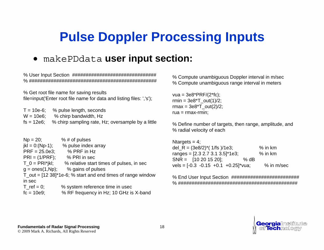
Pulse Doppler Processing Inputs• makePDdata user input section:
% User Input Section ############################### % Compute unambiguous Doppler interval in m/sec% ###############################################
% Get root file name for saving resultsfile=input('Enter root file name for data and listing files: ','s');
T 10e 6 % p lse length seconds
% Compute unambiguous Doppler interval in m/sec% Compute unambiguous range interval in meters
vua = 3e8*PRF/(2*fc);rmin = 3e8*T_out(1)/2;rmax = 3e8*T_out(2)/2;
T = 10e-6; % pulse length, secondsW = 10e6; % chirp bandwidth, Hzfs = 12e6; % chirp sampling rate, Hz; oversample by a little
Np = 20; % # of pulses
rua = rmax-rmin;
% Define number of targets, then range, amplitude, and% radial velocity of each
Ntargets 4Np 20; % # of pulsesjkl = 0:(Np-1); % pulse index arrayPRF = 25.0e3; % PRF in HzPRI = (1/PRF); % PRI in secT_0 = PRI*jkl; % relative start times of pulses, in secg = ones(1,Np); % gains of pulses
Ntargets = 4;del_R = (3e8/2)*( 1/fs )/1e3; % in kmranges = [2.3 2.7 3.1 3.5]*1e3; % in kmSNR = [10 20 15 20]; % dBvels = [-0.3 -0.15 +0.1 +0.25]*vua; % in m/sec
T_out = [12 38]*1e-6; % start and end times of range window in secT_ref = 0; % system reference time in usecfc = 10e9; % RF frequency in Hz; 10 GHz is X-band
% End User Input Section #########################% ############################################
Fundamentals of Radar Signal Processing© 2009 Mark A. Richards, All Rights Reserved
18

Pulse Doppler Processing Outputs - 1
35
40NONCOHERENTLY INTEGRATED RANGE TRACE
20
25
30
pow
er
-10
0
RANGE-DOPPLER PLOT OF UNPROCESSED DATA
1.5 2 2.5 3 3.5 4 4.5 5 5.5 615
range bin
80
-70
-60
-50
-40
-30
-20
RANGE-DOPPLER CONTOUR PLOT OF UNPROCESSED DATA
-200-150
-100-50
050
100150
200
1
2
3
4
5
6-80
velocity (m/s)range (km)
e (k
m) 4
4.5
5
5.5
rang
e
2
2.5
3
3.5
Fundamentals of Radar Signal Processing© 2009 Mark A. Richards, All Rights Reserved
19
velocity (m/s)-150 -100 -50 0 50 100 150

Pulse Doppler Processing Outputs - 2
20
-10
0
RANGE-DOPPLER PLOT OF CLUTTER-CANCELLED DATA RANGE-DOPPLER CONTOUR PLOT OF CLUTTER-CANCELLED DATA
4 5
5
5.5
-80
-70
-60
-50
-40
-30
-20
rang
e (k
m)
3
3.5
4
4.5
-200-150
-100-50
050
100150
200
1
2
3
4
5
6-90
velocity (m/s)range (km)velocity (m/s)
-150 -100 -50 0 50 100 150
2
2.5
3
Fundamentals of Radar Signal Processing© 2009 Mark A. Richards, All Rights Reserved
20

Pulse Doppler Processing Outputs - 3RANGE-DOPPLER CONTOUR PLOT OF CLUTTER-CANCELLED DATA
5
5.5
RANGE-DOPPLER CONTOUR PLOT OF FULLY-PROCESSED DATA
3.5
4
rang
e (k
m)
3.5
4
4.5
rang
e (k
m)
2
2.5
3
-150 -100 -50 0 50 100 150
2
2.5
3
-150 -100 -50 0 50 100 150
0.5
1
1.5
velocity (m/s) velocity (m/s)
-40
-20
0MAXIMUM DOPPLER RESPONSE VS. RANGE
-100
-80
-60
-40
pow
er (d
B)
Fundamentals of Radar Signal Processing© 2009 Mark A. Richards, All Rights Reserved
21
0 0.5 1 1.5 2 2.5 3 3.5 4 4.5-120
range (km)

Doppler Beam Sharpening Imaging - 1• Closely related to the pulse Doppler demonstration and project• Imaging of a user-specified array of point scatterers
T t• Two stages– makeSARdata_DBS creates a fast-time/slow-time data matrix that
will support the desired scenario– procSARdata DBS performs the DBS imaging algorithmprocSARdata_DBS performs the DBS imaging algorithm
• Stage 1: Data Creation• >> edit makeSARdata DBS>> edit makeSARdata_DBS
– Set all simulation parameters by editing input section of makeSARdata_DBS.m
• >> makeSARdata_DBS– To create data set for processing– Output in file.mat
• Where file is the “root file name” you specify
Fundamentals of Radar Signal Processing© 2009 Mark A. Richards, All Rights Reserved
22
• Parameters logged in file.lis

Doppler Beam Sharpening Imaging - 2• Stage 2: Image Formation
• >> edit procSARdata_DBS– Set image formation option switches by editing input
section of procSARdata_DBS.m_
• >> procSARdata_DBS to generate DBS imageRange compressed only in Fig 1 window– Range-compressed only in Fig. 1 window
– Fully-formed image in Fig. 2 window– If geometric corrections selected, then
C l d i i Fi 3 i d• Cross-range resampled image in Fig. 3 window• Range curvature-corrected image in Fig. 4 window
Fundamentals of Radar Signal Processing© 2009 Mark A. Richards, All Rights Reserved
23

DBS Demonstration: makesardata_DBS% User input section #################################
% need a file name to store data, e.g. 'myfile' or 'temp' or 'sardata'.% Data will then be in 'myfile.dat', etc.
% Define target locations, one row of (x,R) coordinates per target
% Ranges are relative to the CRP range (Rcrp) above.y ,
file=input('Enter root file name for data and listing files: ','s');
DCR = 20; % cross-range resolution, mDR = 20; % range resolution, mRcrp = 40000; % range to swath center
% coords = [0,0]; % a single point target at the CRP
coords = ... % a grid of 9 point targets[-1000,-1000;-1000,0;Rcrp 40000; % range to swath center
v = 150; % platform velocity, m/sfc = 10e9; % RF frequency in Hzlambda = c/fc; % wavelength, mtau = 5e-6; % pulse length, seconds (bandwidth set by
resolution)
, ;-1000,+1000;0,-1000;0,0;0,+1000;+1000,-1000;resolution)
Daz = 0.2; % antenna azimuth size, mthetaaz = lambda/Daz; % azimuth beamwidth, radiansBWdopp = 2*v/lambda*thetaaz; % slow time Doppler bandwidth, HzLs = 3000; % swath depth, moversample st = 2; % slow time oversample factor; higher makes
1000, 1000;+1000,0;+1000,+1000];
% End user input sectionoversample_st = 2; % slow time oversample factor; higher makes% prettier pictures but larger data sets
oversample_ft = 2; % fast time oversample factor, similar to slow time
% End user input section #####################################
% ###################################################
Fundamentals of Radar Signal Processing© 2009 Mark A. Richards, All Rights Reserved
24

Sample Makesardata_DBS Output
Real Part of Data Matrixx 10-4
2.6
2 65
ast t
ime
(sec
)
2.65
2.7
fa
2.75
pulse number100 200 300 400 500 600
2.8
Fundamentals of Radar Signal Processing© 2009 Mark A. Richards, All Rights Reserved
25

DBS Demonstration: procsardata_DBS• %#######################################################• % User input section ###################################
• % algorithm control parameters• dechirp = false; % use azimuth dechirp step or not
l f 2 % li i D l bi k b tt• oversample_freq = 2; % oversampling in Doppler; bigger makes better• % picture but needs more memory and time• fix_geometry = false; % perform geometric corrections or not
• % Get data file name• file=input('Enter root file name for data file: ','s');
• % End user input section ###############################• % ######################################################
Fundamentals of Radar Signal Processing© 2009 Mark A. Richards, All Rights Reserved
26

Sample Makesardata_DBS Output,No Geometric CorrectionsNo Geometric Corrections
After Range Compression, Before Cross-Range Compression-1.5
-1
Fully Compressed Image
e re
lativ
e to
CR
P (k
m)
-0.5
0
0.5
y p g-1.5
-1
rang
e
1
1.5
2
ve to
CR
P (k
m)
-0.5
0
0 5aperture position (m)
-15 -10 -5 0 5 10 15
rang
e re
lativ 0.5
1
1 5
cross-range (km)-6 -4 -2 0 2 4
1.5
2
Fundamentals of Radar Signal Processing© 2009 Mark A. Richards, All Rights Reserved
27
g ( )

Sample Makesardata_DBS Outputwith Geometric Correctionswith Geometric Corrections
Resampled and Range-Shifted Image-1.5
-1
-0.5
lativ
e to
CR
P (k
m)
0
0.5
rang
e re
l
1
1.5
cross range (km)-6 -4 -2 0 2 4 6
2
Fundamentals of Radar Signal Processing© 2009 Mark A. Richards, All Rights Reserved
28
cross-range (km)

Sample procSARdata_DBS Images,with and without Azimuth Dechirpt a d t out ut ec p
• Azimuth dechirp not needed if• Consider R = 40 km, λ = 3 cm, ΔCR = rm
Violates limit which is about 17 m in this case
2CR RλΔ ≥
– Violates limit, which is about 17 m in this case • Generate new data with ΔCR = 5 m, etc.
– Process with requency oversample = 4 for good mainlobe definitionF ll C d I
m)
Fully Compressed Image
-1.04
-1.02
m)
Fully Compressed Image
-1.04
-1.02
-1
rang
e re
lativ
e to
CR
P (k
m -1
-0.98
-0.96
rang
e re
lativ
e to
CR
P (k
m
-0.98
-0.96
0 94
cross-range (km)-1.15 -1.1 -1.05 -1 -0.95 -0.9 -0.85
-0.94
-0.92
cross-range (km)-1.1 -1.05 -1 -0.95 -0.9
-0.94
-0.92
N A i th D hi
Fundamentals of Radar Signal Processing© 2009 Mark A. Richards, All Rights Reserved
29
No Azimuth Dechirp: Cross-Range Smearing
With Azimuth Dechirp:Cross-Range Resolution Goal Met

Adaptive Beamformer• Simple demonstration of four different beamformer patterns in
an environment with two jammersN d ti (fi d) b f– Non-adaptive (fixed) beamformer
– fully-adaptive beamformer using weights– “distortionless” beamformer
P t DFT (b ) b f
-1 *Ih = S t
– Post-DFT (beamspace) beamformer
• >> edit beamform
– Set all parameters by editing input section of beamform.m– RF, jammer AOAs, powers– Array parameters– Use -30 dB Taylor weighting (or not)
• >> beamform
Fundamentals of Radar Signal Processing© 2009 Mark A. Richards, All Rights Reserved
30
– Four different patterns in four figure windows

Adaptive Beamformer beamform%%%%%%%%%%%%%%%%%%%%%%%%%%%%%%%%%%%%%%%%%%%%%%%%%%%%%%% User Input Section
lambda = 0.03; % wavelengthgd = lambda/2; % element spacingdl = d/lambda;N = 16; % # of array elementsaoa_max = asin(1/2/dl); % maximum "real space" AOA (radians)
i d f l % t f lwindow_on = false; % true or false
Nangle = 1000; % # of angles for evaluating beam patternNm1 = Nangle-1;
t_aoa = pi/180*(0); % target AOA (radians)j_aoa1 = pi/180*(18); % jammer #1 AOA (radians)j_aoa2 = pi/180*(-33); % jammer #2 AOA (radians)
SNR = 0; % signal to noise ratio (dB)JSR1 = +50; % jammer #1 to noise ratio (dB)JSR2 = +30; % jammer #2 to noise ratio (dB)
% End user input section
Fundamentals of Radar Signal Processing© 2009 Mark A. Richards, All Rights Reserved
31
% End user input section%%%%%%%%%%%%%%%%%%%%%%%%%%%%%%%%%%%%%%%%%%%%%%%%%%%%%%

Outputs from beamform, Both Jammers in the Sidelobes No Weightingin the Sidelobes, No Weighting
-10
0
B)
Fully Adaptive Array Pattern
-10
0
B)
Unadapted Array Pattern
-50
-40
-30
-20
Nor
mal
ized
Arra
y R
espo
nse
(dB
-50
-40
-30
-20
Nor
mal
ized
Arra
y R
espo
nse
(dB
Di t ti l B f A P tt
-80 -60 -40 -20 0 20 40 60 80-60
Angle of Arrival (degrees)-80 -60 -40 -20 0 20 40 60 80
-60
Angle of Arrival (degrees)
-20
-10
0
Res
pons
e (d
B)
Distortionless Beamformer Array Pattern
30
-20
-10
0
Res
pons
e (d
B)
Post-DFT (Beamspace) Array Pattern
80 60 40 20 0 20 40 60 80-60
-50
-40
-30
Nor
mal
ized
Arra
y
-80 -60 -40 -20 0 20 40 60 80-60
-50
-40
-30
Nor
mal
ized
Arra
y
Fundamentals of Radar Signal Processing© 2009 Mark A. Richards, All Rights Reserved
32
-80 -60 -40 -20 0 20 40 60 80Angle of Arrival (degrees)
80 60 40 20 0 20 40 60 80Angle of Arrival (degrees)

Outputs from beamform, One Jammer in the Mainlobe No Weightingthe Mainlobe , No Weighting
-10
0
)
Unadapted Array Pattern
-10
0
)
Fully Adaptive Array Pattern
-50
-40
-30
-20
Nor
mal
ized
Arra
y R
espo
nse
(dB
)
-50
-40
-30
-20
Nor
mal
ized
Arra
y R
espo
nse
(dB
)
-80 -60 -40 -20 0 20 40 60 80-60
50
Angle of Arrival (degrees)-80 -60 -40 -20 0 20 40 60 80
-60
50
Angle of Arrival (degrees)
Di t ti l B f A P tt P t DFT (B ) A P tt
30
-20
-10
0
y R
espo
nse
(dB
)
Distortionless Beamformer Array Pattern
30
-20
-10
0
y R
espo
nse
(dB
)
Post-DFT (Beamspace) Array Pattern
-80 -60 -40 -20 0 20 40 60 80-60
-50
-40
-30
Nor
mal
ized
Arra
y
-80 -60 -40 -20 0 20 40 60 80-60
-50
-40
-30
Nor
mal
ized
Arra
y
Fundamentals of Radar Signal Processing© 2009 Mark A. Richards, All Rights Reserved
33
80 60 0 0 0 0 0 60 80Angle of Arrival (degrees)
80 60 0 0 0 0 0 60 80Angle of Arrival (degrees)

Student Projects3
1.5
2
2.5x 10⁻³
ty
PDF of RCS vs. Aspect, Large Dominant+Many Case
0.5
1rela
tive
prob
abili
t
0 200 400 600 800 1000 1200 1400 1600 1800 20000
radar cross section (m2)
60
1
30
40
50
ower 0.6
0.7
0.8
0.9
1
e
10
20
30po
0 1
0.2
0.3
0.4
0.5
ampl
itude
Fundamentals of Radar Signal Processing© 2009 Mark A. Richards, All Rights Reserved
34
0 50 100 150 200 250 300 350 4000sample -0.5 -0.4 -0.3 -0.2 -0.1 0 0.1 0.2 0.3 0.4 0.5
0
0.1
normalized frequency (cycles)

Student Projects - 1• “Student projects” are simulation projects intended to illustrate
radar signal behavior and/or teach students to implement simple signal processing algorithmssimple signal processing algorithms
• Included are four project topics– RCS statistics– Linear FM waveform properties and matched filtering– Pulse Doppler processing and detection– CFAR detection
• For each project, the following are provided:p j g p– Example problem assignment in Microsoft Word format– Example problem solution consisting of
• Sample MATLAB code
Fundamentals of Radar Signal Processing© 2009 Mark A. Richards, All Rights Reserved
• Microsoft Word document describing the solution
35

Student Projects - 2• Document note for all projects: Equations in the
problem assignment and solution documents were created in MathType™. MathType is an upgrade to Microsoft’s Equation Editor. It can edit equations created in Equation Editor, however, the converse iscreated in Equation Editor, however, the converse is not true. In addition, MathType may use some fonts or characters not available on machines on which it is not installed Consequently it is recommended that theinstalled. Consequently, it is recommended that the user install MathType if it is desired to work with the student project assignment and solution documents. MathType is available at www.dessci.com/en/products/mathtype/.
Fundamentals of Radar Signal Processing© 2009 Mark A. Richards, All Rights Reserved
36

Student Projects - 3• All projects are self-contained and self-explanatory
using the problem assignment document, except for the pulse Doppler project
Th l D l j t i th t d t b• The pulse Doppler project requires that data be generated by the instructor, to be analyzed by the students.
• The following charts provide some additional detail ti d t f th l D l j t don creating data for the pulse Doppler project and
then using that data in the sample solution.
Fundamentals of Radar Signal Processing© 2009 Mark A. Richards, All Rights Reserved
37

MTI + Pulse Doppler Processing• Place all files in the Pulse Doppler directory in the MATLAB
work directory– Or anywhere on the MATLAB pathOr anywhere on the MATLAB path
• >> edit makedata– Set all parameters by editing input section of makedata.m– Includes noise, clutter, moving targets, and R4
R d RF PRF i d• Radar parameters: RF, PRF, range window• Target SNR, ranges, velocities, #of targets• CNR
• >> makedata>> makedata– To create data set for processing– Output data in file.mat
• Where file is the “root file name” you specifyP t l d i• Parameters logged in file.lis
• >> procdata– To perform MTI + pulse Doppler processing, generate displays
• Input is in same file mat specified in makedata
Fundamentals of Radar Signal Processing© 2009 Mark A. Richards, All Rights Reserved
38
Input is in same file.mat specified in makedata• Program pauses at every graph; hit any key to continue

Create PD Data: makedata% User Input Section ####################################% ####################################################
% Get root file name for saving results
% Compute unambiguous Doppler interval in m/sec% Compute unambiguous range interval in meters
vua = 3e8*PRF/(2*fc);% Get root file name for saving resultsfile=input('Enter root file name for data and listing files: ','s');
T = 10e-6; % pulse length, secondsW = 10e6; % chirp bandwidth, Hz
vua = 3e8*PRF/(2*fc);rmin = 3e8*T_out(1)/2;rmax = 3e8*T_out(2)/2;rua = rmax-rmin;
fs = 12e6; % chirp sampling rate, Hz; oversample by a little
Np = 20; % # of pulsesjkl = 0:(Np 1); % pulse index array
% Define number of targets, then range, amplitude, and% radial velocity of each
Ntargets = 4;del R = (3e8/2)*( 1/fs )/1e3; % in kmjkl = 0:(Np-1); % pulse index array
PRF = 25.0e3; % PRF in HzPRI = (1/PRF); % PRI in secT_0 = PRI*jkl; % relative start times of pulses, in secg = ones(1,Np); % gains of pulses
del_R = (3e8/2)*( 1/fs )/1e3; % in kmranges = [2.3 2.7 3.1 3.5]*1e3; % in kmSNR = [10 20 15 20]; % dBvels = [-0.3 -0.15 +0.1 +0.25]*vua; % in m/sec
g ( p) g pT_out = [12 38]*1e-6; % start and end times of range window in
secT_ref = 0; % system reference time in usecfc = 10e9; % RF frequency in Hz; 10 GHz is X-band
% End User Input Section ###############################% #############################################
Fundamentals of Radar Signal Processing© 2009 Mark A. Richards, All Rights Reserved
39

Final Output from makedata
20
30
10
B)
-10
0
ampl
itude
(dB
30
-20
1.5 2 2.5 3 3.5 4 4.5 5 5.5 6-40
-30
distance (km)
Fundamentals of Radar Signal Processing© 2009 Mark A. Richards, All Rights Reserved
40
distance (km)

Process PD Data: procdata• No parameters to set• Some sample figures:
MAXIMUM DOPPLER RESPONSE VS RANGE
40
-30
-20
-10
0MAXIMUM DOPPLER RESPONSE VS. RANGE
-80
-70
-60
-50
-40
pow
er (d
B)
Fundamentals of Radar Signal Processing© 2009 Mark A. Richards, All Rights Reserved
41
0 0.5 1 1.5 2 2.5 3 3.5 4 4.5-100
-90
range (km)

Missing Pieces?
• Contact Mark Richards by e-mail,Contact Mark Richards by e mail, [email protected]
Fundamentals of Radar Signal Processing© 2009 Mark A. Richards, All Rights Reserved
42