Some Improvements to a Parametric Line Clipping Algorithm Improvements to a...line clipping algorithms that are based on a strict mathematical form.9,10 Our line clipping algorithm

Some Improvements to a Parametric Line Clipping Algorithm

You-Dong Liang†, Brian A. Barsky, Mel Slater‡

Computer Science DivisionUniversity of California

Berkeley, California 94720U.S.A.

This paper presents an improved version of our earlier1, 2 parametric line clipping algo-rithm.

There are two types of improvements. The first involves an initial trivial reject test basedonly on comparisons, and the second is the addition of a test to avoid unnecessary com-putation when the result will not affect the parametric value of the intersection point. Foreach dimension, the mathematics are derived along with geometrical interpretations andthe algorithm is designed. Finally, a performance test is conducted. Both the originaland improved versions of our algorithm are compared to the traditional Sutherland-Cohen3, 4 clipping algorithm.

0. Introduction

Clipping is a basic and important problem in computer graphics. It is the process ofremoving that portion of an image that lies outside a region called the clip window orvisible region.5, 6 One way to classify clipping algorithms is according to the type ofhhhhhhhhhhhhhhh

† Permanent address: Department of Mathematics, Zhejiang University, Hangzhou, Zhejiang People’s Republic of Chi-

na

‡ Permanent address: Department of Computer Science, QMW University of London, Mile End Road, London E1 4NS,

U.K.1 You-Dong Liang and Brian A. Barsky, ‘‘A New Concept and Method for Line Clipping,’’

ACM Transactions on Graphics, Vol. 3, No. 1, January, 1984, pp. 1-22.2 You-Dong Liang and Brian A. Barsky, ‘‘Introducing A New Technique for Line Clipping,’’

pp. 548-559 in Proceedings of the International Conference on Engineering and ComputerGraphics, Beijing, 27 August - 1 September 1984. Also in Journal of Zhejiang University SpecialIssue on Computational Geometry, 1984, pp.1-12.

3 James D. Foley, Andries van Dam, Steven K. Feiner, and John F. Hughes, Computer Graph-ics: Principles and Practice, Addison-Wesley Publishing Company, 1990. Second Edition.

4 William M. Newman and Robert F. Sproull, Principles of Interactive Computer Graphics,McGraw-Hill, 1979. Second edition.



- 2 -

primitive upon which they operate; the type of clipping to be considered in this paper isline clipping.

In the early time of computer graphics, the Sutherland/Cohen7, 8 line clipping algorithmand its coding technique was in common use. In 1984, we proposed a family of efficientline clipping algorithms that are based on a strict mathematical form.9, 10

Our line clipping algorithm employed a parametric representation of the line segment tobe clipped, used minimum and maximum calculations to determine the parametric valuescorresponding to the endpoints of the visible line segment, and developed several newdefinitions for trivial reject to speed up the approach. A similar approach was indepen-dently adopted by Cyrus and Beck11 although that work did not develop the trivial rejectcases that are so important for efficiency.

The method for line clipping that we developed describes clipping in an exact andmathematical form. The basic ideas form the foundation for a family of algorithms fortwo-, three-, and four- (homogeneous coordinates) dimensional line clipping.

One of the features of our algorithm is that it is independent of dimension. The identicalcoded procedure can be used for clipping in any dimension. The applicability of thisalgorithm for different dimensions only requires a different calling sequence for this pro-cedure. This feature is both theoretically interesting and practically convenient. For thisreason, the computation times for our algorithm are fairly constant over the differentdimensions.

At SIGGRAPH’87, Nicholl, Lee, and Nicholl12 presented a very efficient two-dimensional line clipping algorithm that is based on a case-by-case approach and whichimproved upon the existing line clipping algorithms. However, their algorithm is onlyapplicable in two dimensions.

In our algorithm, the line segment to be clipped is mapped into a parametric representa-tion. >From this, a set of conditions is derived that describes the interior of the clippingregion. Observing that these conditions are all of similar form, they are rewritten suchthat the solution to the clipping problem is reduced to a simple max/min expression.

hhhhhhhhhhhhhhh7 James D. Foley, Andries van Dam, Steven K. Feiner, and John F. Hughes, Computer Graph-

ics: Principles and Practice, Addison-Wesley Publishing Company, 1990. Second Edition.8 William M. Newman and Robert F. Sproull, Principles of Interactive Computer Graphics,

McGraw-Hill, 1979. Second edition.9 You-Dong Liang and Brian A. Barsky, ‘‘A New Concept and Method for Line Clipping,’’

ACM Transactions on Graphics, Vol. 3, No. 1, January, 1984, pp. 1-22.10 You-Dong Liang and Brian A. Barsky, ‘‘Introducing A New Technique for Line Clipping,’’

pp. 548-559 in Proceedings of the International Conference on Engineering and ComputerGraphics, Beijing, 27 August - 1 September 1984. Also in Journal of Zhejiang University SpecialIssue on Computational Geometry, 1984, pp.1-12.

11 Mike Cyrus and Jay Beck, ‘‘Generalized Two- and Three-Dimensional Clipping,’’ Comput-ers and Graphics, Vol. 3, No. 1, 1978, pp. 23-28.

12 Tina M. Nicholl, D. T. Lee, and Robin A. Nicholl, ‘‘An Efficient New Algorithm for 2-DLine Clipping: Its Development and Analysis,’’ pp. 253-262 in SIGGRAPH ’87 ConferenceProceedings, ACM, Anaheim, July 27-31, 1987.

- 3 -

Another advantage of our algorithm is that line segments that are invisible are quicklyrejected. In addition, although the three-dimensional and homogeneous coordinate algo-rithms are presented for perspective viewing volumes, it should be noted that it is equallyappropriate for non-perspective viewing volumes, and more generally, for any convexvisible region.

Furthermore, the structure of the algorithm is such that the conditions describing the inte-rior of the clipping region are all of similar form; consequently, these visibility calcula-tions could be processed in parallel.

In this paper, we describe an improved version of this algorithm. There are three types ofimprovements. First, we introduce an initial test for trivial reject, that is, based only oncomparisons between the line endpoints and the clipping boundaries. Second, the origi-nal algorithm employed two different kinds of tests to accomplish subsequent trivialrejects; in the improved version, we add a third type of test for trivial reject. Third, testsare added so as to avoid unnecessary computation when the result will not affect theparametric value of the intersection point.

For each dimension, the mathematics are discussed and the algorithm is designed, andthen a performance test is conducted. Both the original and improved versions of ouralgorithm are compared to the traditional Sutherland-Cohen13, 14 clipping algorithm.Using randomly generated data, the original version of our algorithm showed a 25% to62% improvement compared to the Sutherland-Cohen algorithm and the improved ver-sion of our algorithm had a 46% to 68% improvement over the Sutherland-Cohen algo-rithm.

1. Setting up the Problem in Two, Three, and Four Dimensions

In two-dimensional clipping, lines are clipped against a two-dimensional region calledthe clip window (Figure 1-1). In particular, let the equations of the boundary lines be

y = y top

y = y bottom

x = x right

x = x left

(1.1)

representing the left, right, bottom, and top boundaries, respectively. Using this notation,a two-dimensional point ( x , y ) is inside the window if and only if

y bottom ≤ y ≤ y top

x left ≤ x ≤ x right(1.2)

hhhhhhhhhhhhhhh13 James D. Foley, Andries van Dam, Steven K. Feiner, and John F. Hughes, Computer Graph-

ics: Principles and Practice, Addison-Wesley Publishing Company, 1990. Second Edition.14 William M. Newman and Robert F. Sproull, Principles of Interactive Computer Graphics,

McGraw-Hill, 1979. Second edition.

- 4 -

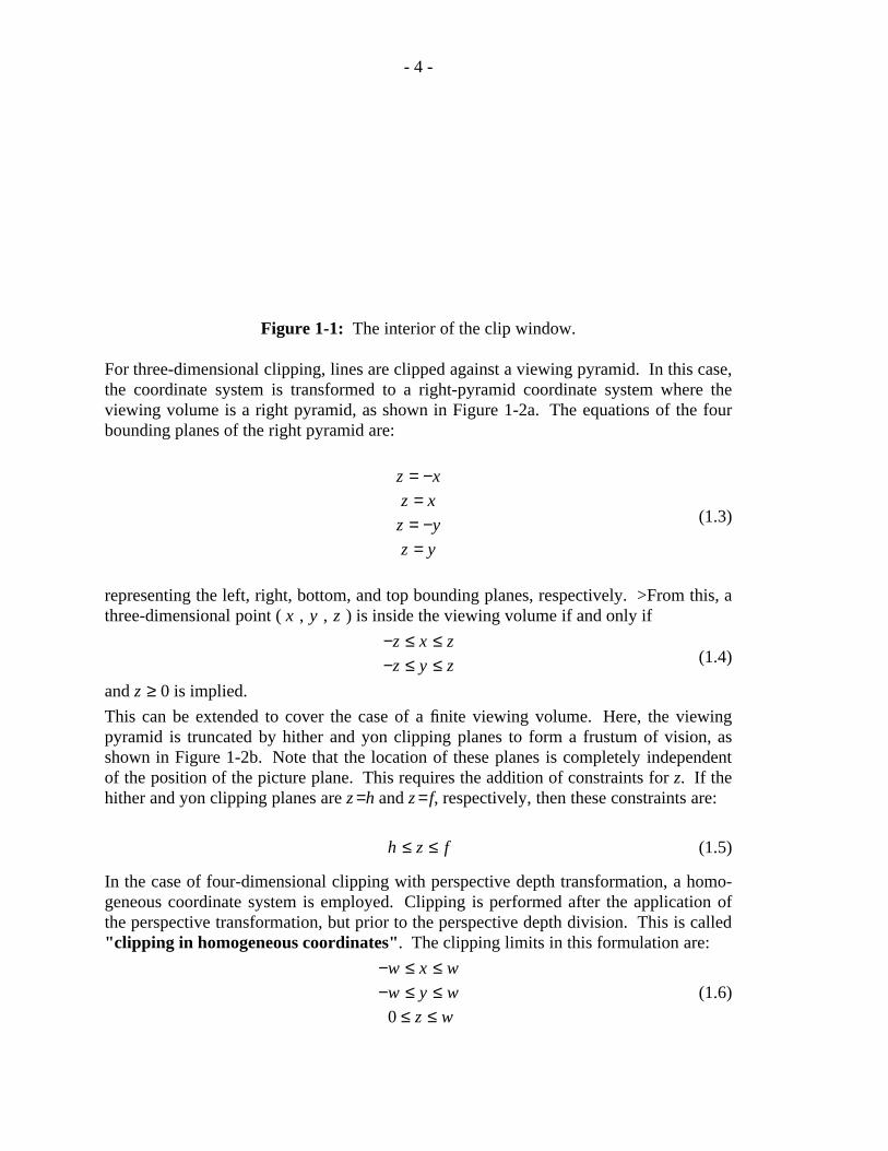
Figure 1-1: The interior of the clip window.

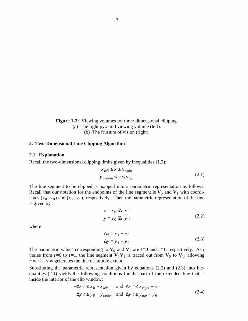
For three-dimensional clipping, lines are clipped against a viewing pyramid. In this case,the coordinate system is transformed to a right-pyramid coordinate system where theviewing volume is a right pyramid, as shown in Figure 1-2a. The equations of the fourbounding planes of the right pyramid are:

z = y

z = −y

z = x

z = −x

(1.3)

representing the left, right, bottom, and top bounding planes, respectively. >From this, athree-dimensional point ( x , y , z ) is inside the viewing volume if and only if

−z ≤ y ≤ z

−z ≤ x ≤ z(1.4)

and z ≥ 0 is implied.

This can be extended to cover the case of a finite viewing volume. Here, the viewingpyramid is truncated by hither and yon clipping planes to form a frustum of vision, asshown in Figure 1-2b. Note that the location of these planes is completely independentof the position of the picture plane. This requires the addition of constraints for z. If thehither and yon clipping planes are z =h and z = f, respectively, then these constraints are:

h ≤ z ≤ f (1.5)

In the case of four-dimensional clipping with perspective depth transformation, a homo-geneous coordinate system is employed. Clipping is performed after the application ofthe perspective transformation, but prior to the perspective depth division. This is called"clipping in homogeneous coordinates". The clipping limits in this formulation are:

0 ≤ z ≤ w

−w ≤ y ≤ w

−w ≤ x ≤ w

(1.6)

- 5 -

Figure 1-2: Viewing volumes for three-dimensional clipping.(a) The right pyramid viewing volume (left).

(b) The frustum of vision (right).

2. Two-Dimensional Line Clipping Algorithm

2.1. Explanation

Recall the two-dimensional clipping limits given by inequalities (1.2):

y bottom ≤ y ≤ y top

x left ≤ x ≤ x right(2.1)

The line segment to be clipped is mapped into a parametric representation as follows.Recall that our notation for the endpoints of the line segment is V0 and V1 with coordi-nates (x 0, y 0) and (x 1, y 1), respectively. Then the parametric representation of the lineis given by

y = y 0 + ∆y t

x = x 0 + ∆x t(2.2)

where

∆y = y 1 − y 0

∆x = x 1 − x 0(2.3)

The parametric values corresponding to V0 and V1 are t =0 and t =1, respectively. As tvaries from t =0 to t =1, the line segment V0V1 is traced out from V0 to V1; allowing− ∞ < t < ∞ generates the line of infinite extent.

Substituting the parametric representation given by equations (2.2) and (2.3) into ine-qualities (2.1) yields the following conditions for the part of the extended line that isinside the interior of the clip window:

−∆y t ≤ y 0 − y bottom

−∆x t ≤ x 0 − x left

and

and

∆y t ≤ y top − y 0

∆x t ≤ x right − x 0(2.4)

- 6 -

Note that these conditions (2.4) are inequalities describing the interior of the clip windowrather than equations defining its boundary.

Observe that inequalities (2.4) are all of similar form; thus, they can be rewritten as

pi t ≤ qi for i=1, 2, 3, 4 (2.5)

where the following notation is used:

p 4 = ∆y

p 3 = −∆y

p 2 = ∆x

p 1 = −∆x

q 4 = y top − y 0

q 3 = y 0 − y bottom

q 2 = x right − x 0

q 1 = x 0 − x left

(2.6)

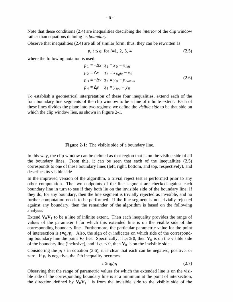
To establish a geometrical interpretation of these four inequalities, extend each of thefour boundary line segments of the clip window to be a line of infinite extent. Each ofthese lines divides the plane into two regions; we define the visible side to be that side onwhich the clip window lies, as shown in Figure 2-1.

Figure 2-1: The visible side of a boundary line.

In this way, the clip window can be defined as that region that is on the visible side of allthe boundary lines. From this, it can be seen that each of the inequalities (2.5)corresponds to one of these boundary lines (left, right, bottom, and top, respectively), anddescribes its visible side.

In the improved version of the algorithm, a trivial reject test is performed prior to anyother computation. The two endpoints of the line segment are checked against eachboundary line in turn to see if they both lie on the invisible side of the boundary line. Ifthey do, for any boundary, then the line segment is trivially rejected as invisible, and nofurther computation needs to be performed. If the line segment is not trivially rejectedagainst any boundary, then the remainder of the algorithm is based on the followinganalysis.

Extend V0V1 to be a line of infinite extent. Then each inequality provides the range ofvalues of the parameter t for which this extended line is on the visible side of thecorresponding boundary line. Furthermore, the particular parametric value for the pointof intersection is t=qi/pi . Also, the sign of qi indicates on which side of the correspond-ing boundary line the point V0 lies. Specifically, if qi ≥ 0, then V0 is on the visible sideof the boundary line (inclusive), and if qi < 0, then V0 is on the invisible side.

Considering the pi’s in equation (2.6), it is clear that each can be negative, positive, orzero. If pi is negative, the i’th inequality becomes

t ≥ qi/pi (2.7)

Observing that the range of parametric values for which the extended line is on the visi-ble side of the corresponding boundary line is at a minimum at the point of intersection,the direction defined by V0V1

hhhhh→is from the invisible side to the visible side of the

- 7 -

boundary line.

Analogously, if pi is positive, the i’th inequality becomes

t ≤ qi/pi (2.8)

Since the parametric range is at a maximum at the point of intersection, the directiondefined by V0V1

hhhhh→must be from the visible side to the invisible side of the corresponding

boundary line.

Finally, if pi is zero, the i’th inequality becomes

0 ≤ qi (2.9)

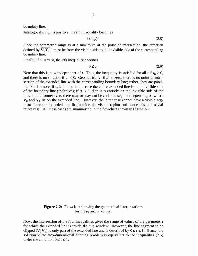
Note that this is now independent of t. Thus, the inequality is satisfied for all t if qi ≥ 0,and there is no solution if qi < 0. Geometrically, if pi is zero, there is no point of inter-section of the extended line with the corresponding boundary line; rather, they are paral-lel. Furthermore, if qi ≥ 0, then in this case the entire extended line is on the visible sideof the boundary line (inclusive); if qi < 0, then it is entirely on the invisible side of theline. In the former case, there may or may not be a visible segment depending on whereV0 and V1 lie on the extended line. However, the latter case cannot have a visible seg-ment since the extended line lies outside the visible region and hence this is a trivialreject case. All these cases are summarized in the flowchart shown in Figure 2-2.

Figure 2-2: Flowchart showing the geometrical interpretationsfor the pi and qi values.

Now, the intersection of the four inequalities gives the range of values of the parameter tfor which the extended line is inside the clip window. However, the line segment to beclipped (V0V1) is only part of the extended line and is described by 0 ≤ t ≤ 1. Hence, thesolution to the two-dimensional clipping problem is equivalent to the inequalities (2.5)under the condition 0 ≤ t ≤ 1.

- 8 -

Solving these inequalities is actually a max/min problem, which can be seen as follows.Recall that t ≥ qi/pi for all i such that pi<0, and that t≥0. Thus,

t ≥ max ({qi/pi c pi<0, i = 1, 2, 3, 4}∪{0}) (2.10)

Analogously, t ≤ qi/pi for all i such that pi>0, and t≤1. Thus,

t ≤ min ({qi/pi c pi>0, i = 1, 2, 3, 4}∪{1}) (2.11)

Finally, if pi=0 in the i’th inequality for some i, then there are two possibilities. If qi ≥ 0,then there is no useful information to be gleaned from this inequality, and this inequalitycan be discarded. If qi < 0, then this is a trivial reject case, and the clipping problem issolved with no further computation needed.

The righthand sides of equations (2.10) and (2.11) are the values of the parameter tcorresponding to the beginning and end of the visible segment, respectively (assumingthere is a visible segment).

Denoting these parametric values as t 0 and t 1,

t 1 = min ({qi/pi c pi>0, i = 1, 2, 3, 4}∪{1})

t 0 = max ({qi/pi c pi<0, i = 1, 2, 3, 4}∪{0})(2.12)

If there is a visible segment, it corresponds to the parametric interval

t 0 ≤ t ≤ t 1 (2.13)

Hence, a necessary condition for a line segment to be at least partially visible is

t 0 ≤ t 1 (2.14)

This is not a sufficient condition because it ignores the possibility of a trivial reject due topi=0 with qi<0. Nonetheless, this yields a sufficient condition for rejection; specifically,if t 0 > t 1, then this is another reject case. The algorithm checks if pi=0 with qi<0 or ift 0 > t 1, in which case the line segment is immediately rejected without further computa-tion.

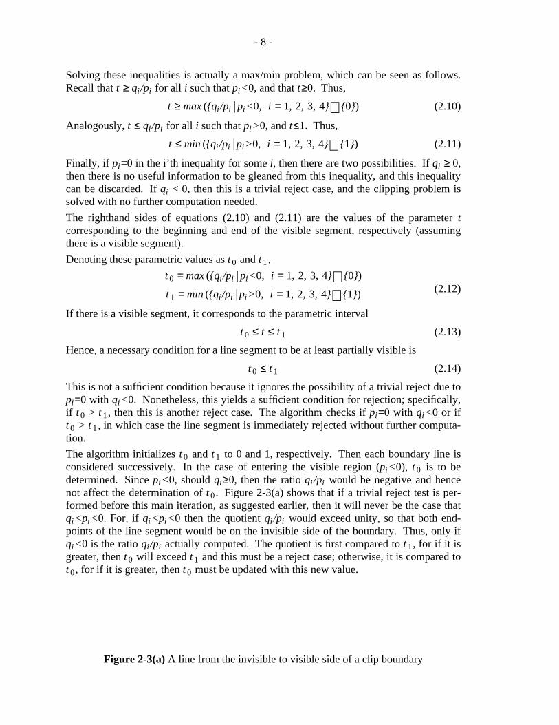
The algorithm initializes t 0 and t 1 to 0 and 1, respectively. Then each boundary line isconsidered successively. In the case of entering the visible region (pi<0), t 0 is to bedetermined. Since pi<0, should qi≥0, then the ratio qi/pi would be negative and hencenot affect the determination of t 0. Figure 2-3(a) shows that if a trivial reject test is per-formed before this main iteration, as suggested earlier, then it will never be the case thatqi<pi<0. For, if qi<pi<0 then the quotient qi/pi would exceed unity, so that both end-points of the line segment would be on the invisible side of the boundary. Thus, only ifqi<0 is the ratio qi/pi actually computed. The quotient is first compared to t 1, for if it isgreater, then t 0 will exceed t 1 and this must be a reject case; otherwise, it is compared tot 0, for if it is greater, then t 0 must be updated with this new value.

Figure 2-3(a) A line from the invisible to visible side of a clip boundary

- 9 -

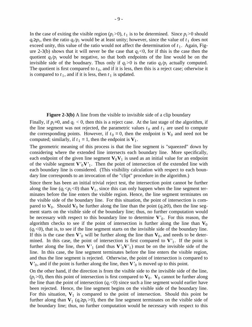
In the case of exiting the visible region (pi>0), t 1 is to be determined. Since pi>0 shouldqi≥pi , then the ratio qi/pi would be at least unity; however, since the value of t 1 does notexceed unity, this value of the ratio would not affect the determination of t 1. Again, Fig-ure 2-3(b) shows that it will never be the case that qi<0, for if this is the case then thequotient qi/pi would be negative, so that both endpoints of the line would be on theinvisible side of the boudnary. Thus only if qi>0 is the ratio qi/pi actually computed.The quotient is first compared to t 0, and if it is less, then this is a reject case; otherwise itis compared to t 1, and if it is less, then t 1 is updated.

Figure 2-3(b) A line from the visible to invisible side of a clip boundary

Finally, if pi=0, and qi < 0, then this is a reject case. At the last stage of the algorithm, ifthe line segment was not rejected, the parametric values t 0 and t 1 are used to computethe corresponding points. However, if t 0 = 0, then the endpoint is V0 and need not becomputed; similarly, if t 1 = 1, then the endpoint is V1.

The geometric meaning of this process is that the line segment is "squeezed" down byconsidering where the extended line intersects each boundary line. More specifically,each endpoint of the given line segment V0V1 is used as an initial value for an endpointof the visible segment V’0V’1. Then the point of intersection of the extended line witheach boundary line is considered. (This visibility calculation with respect to each boun-dary line corresponds to an invocation of the "clipt" procedure in the algorithm.)

Since there has been an initial trivial reject test, the intersection point cannot be furtheralong the line (qi<pi<0) than V1, since this can only happen when the line segment ter-minates before the line enters the visible region. Hence, the line segment terminates onthe visible side of the boundary line. For this situation, the point of intersection is com-pared to V0. Should V0 be further along the line than the point (qi≥0), then the line seg-ment starts on the visible side of the boundary line; thus, no further computation wouldbe necessary with respect to this boundary line to determine V’0. For this reason, thealgorithm checks to see if the point of intersection is further along the line than V0(qi<0), that is, to see if the line segment starts on the invisible side of the boundary line.If this is the case then V’0 will be further along the line than V0, and needs to be deter-mined. In this case, the point of intersection is first compared to V’1. If the point isfurther along the line, then V’1 (and thus V’0V’1) must be on the invisible side of theline. In this case, the line segment terminates before the line enters the visible region,and thus the line segment is rejected. Otherwise, the point of intersection is compared toV’0, and if the point is further along the line, then V’0 is moved up to this point.

On the other hand, if the direction is from the visible side to the invisible side of the line,(pi>0), then this point of intersection is first compared to V0. V0 cannot be further alongthe line than the point of intersection (qi<0) since such a line segment would earlier havebeen rejected. Hence, the line segment begins on the visible side of the boundary line.For this situation, V1 is compared to the point of intersection. Should this point befurther along than V1 (qi≥pi>0), then the line segment terminates on the visible side ofthe boundary line; thus, no further computation would be necessary with respect to this

- 10 -

boundary line to determine V’1. For this reason, the algorithm examines V1 to see if itis further along than the point of intersection (0≤qi<pi), that is, to check that the line seg-ment terminates on the invisible side of the boundary line. If this is the case then V’1will precede V1 along the line, and needs to be determined. In this case, the point ofintersection is first compared to V’0. If V’0 is further along the line than the point, thenV’0 (and thus V’0V’1) must be on the invisible side of the boundary line. In this case,the line segment does not begin until after the line exits the visible region, and thus theline segment is rejected. Otherwise, the point of intersection is compared to V’1, and ifV’1 is further along the line than the point, then V’1 is moved down to this point.

Finally, if the extended line is parallel to the boundary line and on its invisible side, theline segment is rejected. At the end of the algorithm, if the line segment was notrejected, V’0 and V’1 are the required the endpoints of the visible segment. One pro-gramming detail is that assuming V’0 overwrites V0, then V’1 must be assigned prior toV’0 since the computation of V’1 is dependent on V0.

On a final mathematical note, although it is not necessary for the algorithm, inequality(2.14) can be modified to be a necessary and sufficient condition for a line segment to beat least partially visible. This requires the inclusion of the pi=0 case (line segment paral-lel to the corresponding boundary line). This case can be combined with that for pi<0 ifqi/pi is defined as follows:

qi/pi =IKL+∞ if pi = 0 and qi ≥ 0

−∞ if pi = 0 and qi < 0(2.15)

Then the necessary and sufficient condition is

t 0 ≤ t1* (2.16)

where

t1* = min ({qi/pi c pi ≥ 0, i = 1, 2, 3, 4}∪{1}). (2.17)

2.2. Algorithm

The improved algorithm to perform two-dimensional line clipping is as follows:

(* Clip 2-d line segment with endpoints (x0, y0) and (x1, y1). *)(* The clip window is xleft <= x <= xright and ybottom <= y <= ytop. *)

procedure clip2d (var x0, y0, x1, y1: real; var visible: Boolean);label 1;var t0, t1: real;

deltax, deltay: real;

function clipt ((* value *) p, q: real; var t0, t1: real): Boolean;var

r : real;accept : Boolean;

begin (* clipt *)accept := true;

- 11 -

if p < 0 then begin (* entering visible region, so compute t0 *)if q < 0 then begin (* t0 will be nonnegative, so continue *)

r := q / p;if r > t1 then accept := false (* t0 will exceed t1, so reject *)else if r > t0 then t0 := r (* t0 is max of r’s *)

end (* t0 will be nonnegative, so continue *)end (* entering visible region, so compute t0 *)

else if p > 0 then begin (* exiting visible region, so compute t1 *)if q < p then begin (* t1 will be <= 1, so continue *)

r := q / p;if r < t0 then accept := false (* t1 will be <= t0, so reject *)else if r < t1 then t1 := r (* t1 is min of r’s *)

end (* t1 will be <= 1, so continue *)end (* exiting visible region, so compute t1 *)

else (* p=0 *) if q < 0 then accept := false; (* line parallel and outside *)

clipt := acceptend (* function clipt *);

begin (* clip2d *)if (((x0 < xleft) and (x1 < xleft)) or((x0 > xright) and (x1 > xright)) or((y0 < ybottom) and (y1 < ybottom)) or((y0 > ytop) and (y1 > ytop))) then

begin (* sc trivial reject *)visible := false;goto 1;

end; (* sc trivial reject *)

begin (* not trivial reject *)visible := false;

t0 := 0;t1 := 1;deltax := x1 - x0;

if clipt (- deltax, x0 - xleft, t0, t1) (* left *) thenif clipt (deltax, xright - x0, t0, t1) (* right *) then begin

deltay := y1 - y0;if clipt (- deltay, y0 - ybottom, t0, t1) (* bottom *) then

if clipt (deltay, ytop - y0, t0, t1) (* top *) then begin (* compute coordinates *)if t1 < 1 then begin (* compute V1’ *)

x1 := x0 + t1 * deltax;y1 := y0 + t1 * deltay

end (* compute V1’ *);if t0 > 0 then begin (* compute V0’ *)

x0 := x0 + t0 * deltax;

- 12 -

y0 := y0 + t0 * deltayend (* compute V0’ *);visible := true

end; (* compute coordinates *)end

end; (* not trivial reject *)1: null;

end (* clip2d *);

3. Three-Dimensional Line Clipping Algorithm

3.1. Explanation

The three-dimensional line clipping algorithm is analogous to the method developed inSection 2. First, a trivial accept test is performed. This involves checking each endpointof the line segment to be clipped against each bounding plane of the viewing volume. Ifboth endpoints lie on the outside of at least one bounding plane, then the line segment istrivially rejected. Otherwise, the line segment is mapped into a parametric representa-tion. Denoting the endpoints of the line segment as V0 and V1 with coordinates(x 0, y 0, z 0) and (x 1, y 1, z 1), respectively, then the parametric representation of the lineis given by equations (2.2) and (2.3) with the addition of the following equation:

z = z 0 + ∆z t (3.1)

where

∆z = z 1 − z 0 (3.2)

Recall the clipping limits for the right-pyramid viewing volume given by inequalities(1.4):

−z ≤ y ≤ z

−z ≤ x ≤ z(3.3)

Substituting the parametric representation for x and y given by equations (3.1) and (3.2)into inequalities (3.3) yields the following conditions for the part of the extended line thatis inside the volume of the clip window:

−(∆y + ∆z) t ≤ y 0 + z 0 and (∆y − ∆z) t ≤ z 0 − y 0

−(∆x + ∆z) t ≤ x 0 + z 0 and (∆x − ∆z) t ≤ z 0 − x 0(3.4)

The inequalities (3.4) can be rewritten in the form of inequalities (2.7). Specifically,

pi t ≤ qi for i = 1, 2, 3, 4 (3.5)

where the following notation is used:

p 4 = ∆y − ∆z

p 3 = −(∆y + ∆z)

p 2 = ∆x − ∆z

p 1 = −(∆x + ∆z)

q 4 = z 0 − y 0

q 3 = y 0 + z 0

q 2 = z 0 − x 0

q 1 = x 0 + z 0

top

bottom

right

left

(3.6)

The geometrical interpretation of these four inequalities is analogous to that given for thetwo-dimensional case. Extend each of the four bounding sides of the viewing pyramid to

- 13 -

be an (infinite) plane. Then, each of these bounding planes divides the three-space intotwo regions. The visible side is the side on which the viewing pyramid lies. In this way,the viewing pyramid can be defined as that volume that is on the visible side of all thebounding planes. From this, it can be seen that each of the inequalities (3.5) correspondsto one of these planes (left, right, bottom, and top, respectively), and describes its visibleside. To be more specific, extend V0V1 to be a line of infinite extent. Then each ine-quality provides the range of values of the parameter t for which this extended line is onthe visible side of the corresponding plane. Furthermore, the particular parametric valuefor the point of intersection is t=qi/pi . Also, the sign of qi indicates on which side of thecorresponding bounding plane the point V0 lies. Specifically, if qi ≥ 0, then V0 is on thevisible side of the bounding plane (inclusive), and if qi < 0, then V0 is on the invisibleside.

Now, it is readily verified that three of the pi coefficients are linearly independent sincethey satisfy only one linear relation:

p 1 + p 2 − p 3 − p 4 =0

This equation can be solved for any one of the coefficients in terms of the other threeindependent ones. Thus, there is no restriction on the sign of any of the four pi’s.

If pi is negative, the i’th inequality becomes

t ≥ qi/pi (3.7)

Since the range of parametric values for which the extended line is on the visible side ofthe corresponding plane is at a minimum at the point of intersection, the direction definedby V0V1

hhhhh→is from the invisible side to the visible side of the plane.

Analogously, if pi is positive, the i’th inequality becomes

t ≤ qi/pi (3.8)

and the direction defined by V0V1

hhhhh→is from the visible side to the invisible side of the

plane.

Finally, if pi is zero, the i’th inequality becomes

0 ≤ qi (3.9)

Since inequality (3.9) is independent of t, it is satisfied for all t if qi ≥ 0, and there is nosolution if qi < 0. Geometrically, if pi is zero, there is no point of intersection of theextended line with the corresponding plane; rather, the extended line is parallel to theplane. Furthermore, if qi ≥ 0, then in this case the entire extended line is on the visibleside of the plane (inclusive); if qi < 0, then it is entirely on the invisible side of the plane.In the former case, there may or may not be a visible segment depending on where V0and V1 lie on the extended line. However, the latter case cannot have a visible segmentsince the extended line lies outside the viewing volume and hence this is a trivial rejectcase.

Now, the intersection of the four inequalities gives the range of values of the parameter tfor which the extended line is inside the viewing pyramid. However, the line segment tobe clipped (V0V1) is only part of the extended line and is described by 0 ≤ t ≤ 1. Hence,the solution to the three-dimensional clipping problem is equivalent to the inequalities(3.5) under the condition 0 ≤ t ≤ 1. The algorithm to accomplish this is identical to thatdeveloped in Section 2 except the definitions of the pi’s and qi’s are given by equation

- 14 -

(3.6).

As was described in Section 1, hither and yon clipping planes can be optionally added toform a frustum of vision. This is accomplished by recalling the clipping limits engen-dered by the addition of hither and yon clipping planes which were given by inequalities(1.5):

h ≤ z ≤ f (3.10)

Substituting the parametric representation for z given by equations (3.1) and (3.2) intoinequalities (3.10) yields the following additional two constraints:

−∆z t ≤ z 0 − h (3.11)

and

∆z t ≤ f − z 0 (3.12)

These inequalities can be rewritten in the form of inequalities (3.5) where

p 6 = ∆z

p 5 = −∆z

q 6 = f − z 0

q 5 = z 0 − h(3.13)

The geometric meaning of the three-dimensional clipping process is that the line segmentis "squeezed" down by considering where the extended line intersects each boundingplane. More specifically, each endpoint of the given line segment V0V1 is used as an ini-tial value for an endpoint of the visible segment V’0V’1. Then the point of intersectionof the extended line with each bounding plane is considered.

Since there has been an initial trivial reject test, the intersection point cannot be furtheralong the line (qi<pi<0) than V1, since this can only happen when the line segment ter-minates before the line enters the viewing volume. Hence, the line segment terminateson the visible side of the bounding plane. For this situation, the point of intersection iscompared to V0. Should V0 be further along the line than the point (qi≥0), then the linesegment starts on the visible side of the bounding plane; thus, no further computationwould be necessary with respect to this bounding plane to determine V’0. For this rea-son, the algorithm checks to see if the point of intersection is further along the line thanV0 (qi<0), that is, to see if the line segment starts on the invisible side of the boundingplane. If this is the case then V’0 will be further along the line than V0, and needs to bedetermined. In this case, the point of intersection is first compared to V’1. If the point isfurther along the line, then V’1 (and thus V’0V’1) must be on the invisible side of theplane. In this case, the line segment terminates before the line enters the viewingvolume, and thus the line segment is rejected. Otherwise, the point of intersection iscompared to V’0, and if the point is further along the line, then V’0 is moved up to thispoint.

On the other hand, if the direction is from the visible side to the invisible side of theplane (pi>0), then this point of intersection is first compared to V0. V0 cannot be furtheralong the line than the point of intersection (qi<0), since such a line segment would ear-lier have been rejected. Hence, the line segment begins on the visible side of the bound-ing plane. For this situation, V1 is compared to the point of intersection. Should thispoint be further along than V1 (qi≥pi>0), then the line segment terminates on the visibleside of the bounding plane; thus, no further computation would be necessary with respectto this bounding plane to determine V’1. For this reason, the algorithm examines V1 to

- 15 -

see if it is further along than the point of intersection (0≤qi<pi), that is, to check that theline segment terminates on the invisible side of the bounding plane. If this is the casethen V’1 will precede V1 along the line, and needs to be determined. In this case, thepoint of intersection is first compared to V’0. If V’0 is further along the line than thepoint, then V’0 (and thus V’0V’1) must be on the invisible side of the plane. In this case,the line segment does not begin until after the line exits the viewing volume, and thus theline segment is rejected. Otherwise, the point of intersection is compared to V’1, and ifV’1 is further along the line than the point, then V’1 is moved down to this point.

Finally, if the extended line is parallel to the bounding plane and on its invisible side, theline segment is rejected. At the end of the algorithm, if the line segment was notrejected, V’0 and V’1 are the required the endpoints of the visible segment.

3.2. Algorithm

The improved algorithm to perform three-dimensional line clipping is as follows:

(* Clip 3-d line segment with endpoints (x0, y0, z0) and (x1, y1, z1). *)(* The viewing volume is a frustum of vision with hither and yon clipping. *)(* A viewing volume of a right pyramid with its apex at the origin *)(* without hither and yon clipping can be handled simply by removing *)(* the lines indicated in the algorithm. *)

procedure clip3d (var x0, y0, z0, x1, y1, z1: real; var visible: Boolean);label 1;var

t0, t1: real;deltax, deltay, deltaz: real;

begin (* clip3d *)

if (((x0 > z0) and (x1 > z1)) or((y0 > z0) and (y1 > z1)) or((x0 < -z0) and (x1 < -z1)) or((y0 < -z0) and (y1 < -z1))

(* *) or ((z0 < h) and (z1 < h))(* *) or ((z0 > f) and (z1 > f))

) thenbegin (* trivial reject *)visible := false;goto 1;

end; (* trivial reject *)


t0 := 0;t1 := 1;deltax := x1 - x0;deltaz := z1 - z0;

- 16 -

if clipt (- deltax - deltaz, x0 + z0, t0, t1) (* left *) thenif clipt (deltax - deltaz, z0 - x0, t0, t1) (* right *) then begin

deltay := y1 - y0;if clipt (- deltay - deltaz, y0 + z0, t0, t1) (* bottom *) then

if clipt (deltay - deltaz, z0 - y0, t0, t1) (* top *) then(* *) if clipt (- deltaz, z0 - h, t0, t1) (* hither *) then(* *) if clipt (deltaz, f - z0, t0, t1) (* yon *) then

begin (* compute coordinates *)if t1 < 1 then begin (* compute V1’ *)x1 := x0 + t1 * deltax;y1 := y0 + t1 * deltay;z1 := z0 + t1 * deltaz

end (* compute V1’ *);if t0 > 0 then begin (* compute V0’ *)x0 := x0 + t0 * deltax;y0 := y0 + t0 * deltay;z0 := z0 + t0 * deltaz

end (* compute V0’ *);visible := true

end (* compute coordinates *)end

end; (* not trivial reject *)1: null;

end (* clip3d *);

where function clipt is as was defined in Section 2. Hither and yon clipping correspondsto the lines in the algorithm indicated by "(* *)" in the left margin. These lines should beremoved if the viewing volume is not bounded by hither and yon clipping planes.

4. Line Clipping Algorithm for Homogeneous Coordinate Systems

4.1. Explanation

Recall that for line clipping in homogeneous coordinates, clipping is performed after theapplication of the perspective transformation, but prior to the perspective depth division.

The method of Section 3 can be easily extended to handle this case. First, a trivial rejecttest is performed. If both endpoints lie on the outside of at least one bounding plane,then the line segment is trivially rejected. Otherwise, the line segment is mapped into aparametric representation. Denoting the endpoints of the line segment asV0 (x 0, y 0, z 0, w 0) and V1(x 1, y 1, z 1, w 1), then the parametric representation of theline is given by equations (2.2), (2.3), (3.1), and (3.2) with the addition of the followingequation:

w = w 0 + ∆w t (4.1)

where

∆w = w 1 − w 0 (4.2)

- 17 -

Substituting this parametric representation into inequalities (1.6) yields the followingconditions for the part of the extended line that is inside the frustum of vision:

−∆z t ≤ z 0 and (∆z−∆w) t ≤ w 0 − z 0

−(∆y+∆w) t ≤ y 0 + w 0 and (∆y−∆w) t ≤ w 0 − y 0

−(∆x+∆w) t ≤ x 0 + w 0 and (∆x−∆w) t ≤ w 0 − x 0

(4.3)

Again, these conditions are inequalities describing the interior of the clipping volumerather than equations defining its boundary. The six inequalities (4.3) can be rewritten inthe form of inequalities (3.4) with i = 1, 2, ..., 6. Specifically,

pi t ≤ qi for i=1, 2, ..., 6 (4.4)

where

p 6 = ∆z − ∆w

p 5 = −∆z

p 4 = ∆y − ∆w

p 3 = −(∆y + ∆w)

p 2 = ∆x − ∆w

p 1 = −(∆x + ∆w)

q 6 = w 0 − z 0

q 5 = z 0

q 4 = w 0 − y 0

q 3 = y 0 + w 0

q 2 = w 0 − x 0

q 1 = x 0 + w 0

yon

hither

top

bottom

right

left

(4.5)

It can be shown that there are exactly two linear relations satisfied by the pi coefficients:

−p 3 − p 4 + 2p 5 + 2p 6 = 0

p 1 + p 2 − p 5 − p 6 = 0(4.6)

Thus, four of the coefficients are independent and hence there is no restriction on the signof any of the six pi ’s.

Analogous to the method explained in Section 3, clipping using homogeneous coordinatesystems is accomplished by solving the inequalities (4.4) under the condition 0≤t≤1. Thealgorithm is similar to that given in Section 3, except now there are six inequalities to beconsidered, and the pi’s and qi’s are defined by equation (4.5).

4.2. Algorithm

The improved algorithm to perform homogeneous line clipping is as follows:

(* Clip 4-d line segment with endpoints (x0,y0,z0,w0) and (x1,y1,z1,w1). *)(* The viewing volume is a frustum of vision in three-space with hither *)(* and yon clipping. *)

procedure clip4d (var x0, y0, z0, w0, x1, y1, z1, w1: real;var visible: boolean);

label 1;var

t0, t1: real;deltax, deltay, deltaz, deltaw: real;

begin (* clip4d *)

- 18 -

if (((x0 > z0) and (x1 > z1)) or((y0 > z0) and (y1 > z1)) or((x0 < -z0) and (x1 < -z1)) or((y0 < -z0) and (y1 < -z1)) or((z0 < h) and (z1 < h)) or((z0 > f) and (z1 > f))) then

begin (* trivial reject *)visible := false;goto 1;

end; (* trivial reject *)


t0 := 0;t1 := 1;deltax := x1 - x0;deltaw := w1 - w0;if clipt (- deltax - deltaw, x0 + w0, t0, t1) (* left *) then

if clipt (deltax - deltaw, w0 - x0, t0, t1) (* right *) then begindeltay := y1 - y0;if clipt (- deltay - deltaw, y0 + w0, t0, t1) (* bottom *) then

if clipt (deltay - deltaw, w0 - y0, t0, t1) (* top *) then begindeltaz := z1 - z0;if clipt (- deltaz, z0, t0, t1) (* hither *) then

if clipt (deltaz - deltaw, w0 - z0, t0, t1) (* yon *) thenbegin (* compute coordinates *)if t1 < 1 then begin (* compute V1’ *)

x1 := x0 + t1 * deltax;y1 := y0 + t1 * deltay;z1 := z0 + t1 * deltaz;w1 := w0 + t1 * deltaw

end (* compute V1’ *);if t0 > 0 then begin (* compute V0’ *)

x0 := x0 + t0 * deltax;y0 := y0 + t0 * deltay;z0 := z0 + t0 * deltaz;w0 := w0 + t0 * deltaw

end (* compute V0’ *);visible := true;

end (* compute coordinates *)end

endend (* not trivial reject *);

1: null;end (* clip4d *);

where function clipt is as was defined in Section 2.

- 19 -

5. Performance Tests

The computational complexity of the algorithm is linear in the number of line segmentsto be clipped. The exact requirements are dependent upon the particular data. In gen-eral, the worst case occurs when a line segment is not trivially rejected nor parallel to anyof the boundary lines or planes, and has both of its original endpoints outside the visibleregion. In this case, two intersection points must be computed. This requires a total of12 additions/subtractions, 4 multiplications, and 4 divisions for the two-dimensionalalgorithm; or 19 additions/subtractions, 6 multiplications, and 4 divisions for the three-dimensional algorithm using a viewing pyramid; or 25 additions/subtractions, 8 multipli-cations, and 6 divisions for the homogeneous algorithm using a finite viewing frustum.

The improved algorithm was compared to the original version of our algorithm as well asto the traditional Sutherland-Cohen line clipping algorithm for two-dimensional, three-dimensional, and homogeneous clipping, respectively. In the two-dimensional case, therewas also a comparison with the Nicholl-Lee-Nicholl algorithm using Pascal code sup-plied by the authors of that algorithm. Pascal code for the two-dimensional Sutherland-Cohen algorithm was copied verbatim from pages 66-67 of.15 However, it was found thatthe Pascal code for the traditional Sutherland-Cohen three-dimensional clipping algo-rithm as it appears on page 345 of16 sometimes enters an infinite loop. This is due to thefact that this program was based on an assumption that is not always true. Once it isrecognized that the source of this problem is simply this erroneous assumption, then it isa straightforward matter to correct the program. This was done in17 and it is thiscorrected version that was used in this comparison test. For the Sutherland-Cohen homo-geneous line clipping algorithm, Pascal code was copied verbatim from page 360 of18

For each dimension, the three algorithms were executed on four different sets of data,corresponding to different window sizes, and each containing a thousand randomly gen-erated line segments. The data used for the homogeneous case was identical to that forthe three-dimensional case, except transformed to the homogeneous formulation. Eachline segment was clipped a thousand times to reduce the effects of random variation,resulting in a total of four million clips.

Tests were first performed on a Sun 3/160 with a floating point coprocessor in Pascalunder Berkeley UNIX. In the two-dimensional case, the Sutherland/Cohen algorithmused an average of 1486 seconds, while the original version of our algorithm required anaverage of 1213 seconds (an 18% improvement) and the improved version of our algo-rithm used an average of 1074 seconds (a 28% improvement). The Nicholl-Lee-Nichollalgorithm was slightly faster (1059 seconds), in percentage terms also 28%. For clippingin three-dimensions against a viewing pyramid, the Sutherland/Cohen algorithm used anaverage of 1486 seconds, while the original version of our algorithm required an averageof 1266 seconds (a 15% improvement) and the improved version of our algorithm usedhhhhhhhhhhhhhhh



17 You-Dong Liang and Brian A. Barsky, ‘‘A New Concept and Method for Line Clipping,’’ACM Transactions on Graphics, Vol. 3, No. 1, January, 1984, pp. 1-22.


- 20 -

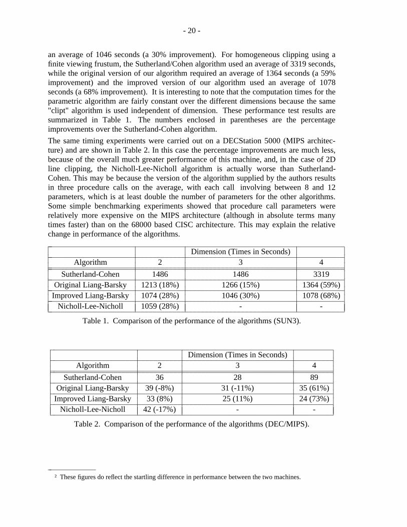
an average of 1046 seconds (a 30% improvement). For homogeneous clipping using afinite viewing frustum, the Sutherland/Cohen algorithm used an average of 3319 seconds,while the original version of our algorithm required an average of 1364 seconds (a 59%improvement) and the improved version of our algorithm used an average of 1078seconds (a 68% improvement). It is interesting to note that the computation times for theparametric algorithm are fairly constant over the different dimensions because the same"clipt" algorithm is used independent of dimension. These performance test results aresummarized in Table 1. The numbers enclosed in parentheses are the percentageimprovements over the Sutherland-Cohen algorithm.

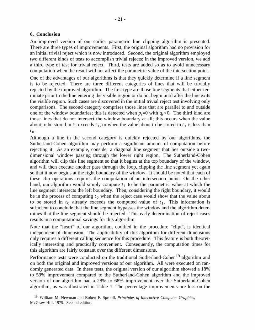
The same timing experiments were carried out on a DECStation 5000 (MIPS architec-ture) and are shown in Table 2. In this case the percentage improvements are much less,because of the overall much greater performance of this machine, and, in the case of 2Dline clipping, the Nicholl-Lee-Nicholl algorithm is actually worse than Sutherland-Cohen. This may be because the version of the algorithm supplied by the authors resultsin three procedure calls on the average, with each call involving between 8 and 12parameters, which is at least double the number of parameters for the other algorithms.Some simple benchmarking experiments showed that procedure call parameters wererelatively more expensive on the MIPS architecture (although in absolute terms manytimes faster) than on the 68000 based CISC architecture. This may explain the relativechange in performance of the algorithms.iiiiiiiiiiiiiiiiiiiiiiiiiiiiiiiiiiiiiiiiiiiiiiiiiiiiiiiiiiiiiiiiiiiiiiiiiii

Dimension (Times in Seconds)iiiiiiiiiiiiiiiiiiiiiiiiiiiiiiiiiiiiiiiiiiiiiiiiiiiiiiiiiiiiiiiiiiiiiiiiiiiAlgorithm 2 3 4iiiiiiiiiiiiiiiiiiiiiiiiiiiiiiiiiiiiiiiiiiiiiiiiiiiiiiiiiiiiiiiiiiiiiiiiiiiiiiiiiiiiiiiiiiiiiiiiiiiiiiiiiiiiiiiiiiiiiiiiiiiiiiiiiiiiiiiiiiiiiiiiiiiiii

Sutherland-Cohen 1486 1486 3319iiiiiiiiiiiiiiiiiiiiiiiiiiiiiiiiiiiiiiiiiiiiiiiiiiiiiiiiiiiiiiiiiiiiiiiiiiiOriginal Liang-Barsky 1213 (18%) 1266 (15%) 1364 (59%)iiiiiiiiiiiiiiiiiiiiiiiiiiiiiiiiiiiiiiiiiiiiiiiiiiiiiiiiiiiiiiiiiiiiiiiiiii

Improved Liang-Barsky 1074 (28%) 1046 (30%) 1078 (68%)iiiiiiiiiiiiiiiiiiiiiiiiiiiiiiiiiiiiiiiiiiiiiiiiiiiiiiiiiiiiiiiiiiiiiiiiiiiNicholl-Lee-Nicholl 1059 (28%) - -iiiiiiiiiiiiiiiiiiiiiiiiiiiiiiiiiiiiiiiiiiiiiiiiiiiiiiiiiiiiiiiiiiiiiiiiiiicc

ccccccc

ccccccccc

ccccccccc

ccccccccc

ccccccccc

Table 1. Comparison of the performance of the algorithms (SUN3).

iiiiiiiiiiiiiiiiiiiiiiiiiiiiiiiiiiiiiiiiiiiiiiiiiiiiiiiiiiiiiiiiiiiiiiiDimension (Times in Seconds)iiiiiiiiiiiiiiiiiiiiiiiiiiiiiiiiiiiiiiiiiiiiiiiiiiiiiiiiiiiiiiiiiiiiiii

Algorithm 2 3 4iiiiiiiiiiiiiiiiiiiiiiiiiiiiiiiiiiiiiiiiiiiiiiiiiiiiiiiiiiiiiiiiiiiiiiiiiiiiiiiiiiiiiiiiiiiiiiiiiiiiiiiiiiiiiiiiiiiiiiiiiiiiiiiiiiiiiiiiiiiiiiSutherland-Cohen 36 28 89iiiiiiiiiiiiiiiiiiiiiiiiiiiiiiiiiiiiiiiiiiiiiiiiiiiiiiiiiiiiiiiiiiiiiii

Original Liang-Barsky 39 (-8%) 31 (-11%) 35 (61%)iiiiiiiiiiiiiiiiiiiiiiiiiiiiiiiiiiiiiiiiiiiiiiiiiiiiiiiiiiiiiiiiiiiiiiiImproved Liang-Barsky 33 (8%) 25 (11%) 24 (73%)iiiiiiiiiiiiiiiiiiiiiiiiiiiiiiiiiiiiiiiiiiiiiiiiiiiiiiiiiiiiiiiiiiiiiii

Nicholl-Lee-Nicholl 42 (-17%) - -iiiiiiiiiiiiiiiiiiiiiiiiiiiiiiiiiiiiiiiiiiiiiiiiiiiiiiiiiiiiiiiiiiiiiiiccccccccc

ccccccccc

ccccccccc

ccccccccc

ccccccccc

Table 2. Comparison of the performance of the algorithms (DEC/MIPS).

hhhhhhhhhhhhhhh† These figures do reflect the startling difference in performance between the two machines.

- 21 -

6. Conclusion

An improved version of our earlier parametric line clipping algorithm is presented.There are three types of improvements. First, the original algorithm had no provision foran initial trivial reject which is now introduced. Second, the original algorithm employedtwo different kinds of tests to accomplish trivial rejects; in the improved version, we adda third type of test for trivial reject. Third, tests are added so as to avoid unnecessarycomputation when the result will not affect the parametric value of the intersection point.

One of the advantages of our algorithms is that they quickly determine if a line segmentis to be rejected. There are three different categories of lines that will be triviallyrejected by the improved algorithm. The first type are those line segments that either ter-minate prior to the line entering the visible region or do not begin until after the line exitsthe visible region. Such cases are discovered in the initial trivial reject test involving onlycomparisons. The second category comprises those lines that are parallel to and outsideone of the window boundaries; this is detected when pi=0 with qi<0. The third kind arethose lines that do not intersect the window boundary at all; this occurs when the valueabout to be stored in t 0 exceeds t 1, or when the value about to be stored in t 1 is less thant 0.

Although a line in the second category is quickly rejected by our algorithms, theSutherland-Cohen algorithm may perform a significant amount of computation beforerejecting it. As an example, consider a diagonal line segment that lies outside a two-dimensional window passing through the lower right region. The Sutherland-Cohenalgorithm will clip this line segment so that it begins at the top boundary of the window,and will then execute another pass through the loop, clipping the line segment yet againso that it now begins at the right boundary of the window. It should be noted that each ofthese clip operations requires the computation of an intersection point. On the otherhand, our algorithm would simply compute t 1 to be the parametric value at which theline segment intersects the left boundary. Then, considering the right boundary, it wouldbe in the process of computing t 0 when the reject case would show that the value aboutto be stored in t 0 already exceeds the computed value of t 1. This information issufficient to conclude that the line segment bypasses the window and the algorithm deter-mines that the line segment should be rejected. This early determination of reject casesresults in a computational savings for this algorithm.

Note that the "heart" of our algorithm, codified in the procedure "clipt", is identicalindependent of dimension. The applicability of this algorithm for different dimensionsonly requires a different calling sequence for this procedure. This feature is both theoret-ically interesting and practically convenient. Consequently, the computation times forthis algorithm are fairly constant over the different dimensions.

Performance tests were conducted on the traditional Sutherland-Cohen19 algorithm andon both the original and improved versions of our algorithm. All were executed on ran-domly generated data. In these tests, the original version of our algorithm showed a 18%to 59% improvement compared to the Sutherland-Cohen algorithm and the improvedversion of our algorithm had a 28% to 68% improvement over the Sutherland-Cohenalgorithm, as was illustrated in Table 1. The percentage improvements are less on thehhhhhhhhhhhhhhh


- 22 -

DECStation 5000 MIPS machine.

Although the three-dimensional and homogeneous coordinate algorithms were presentedfor perspective viewing volumes, it should be noted that it is equally appropriate fornon-perspective viewing volumes, and more generally, for any convex viewing volume.Since the algorithm computes visibility by taking the intersection of the visible sides of aset infinite lines or planes, this approach is applicable to any convex visible region.

Since the structure of the algorithm is such that the conditions describing the interior ofthe clipping region are all of similar form, these visibility calculations could be processedin parallel.

Acknowledgements

The authors are grateful to Simon Hui, Loretta Willis, and Francis W. Yun for their pro-gramming assistance, to Geoff Voelker for carrying out the simulation experiments, andto Walter N. Brown, Caryn Dombroski and Geoff Voelker for their excellent work infigure preparation. This work was supported in part by a National Science FoundationPresidential Young Investigator Award (number CCR-8451997), and in part by theNational Science Foundation under grant number CCR-9015 874.

rm: remove /usr/tmp/grefer4826?

hhhhhhhhhhhhhhh20 James F. Blinn and Martin E. Newell, ‘‘Clipping Using Homogeneous Coordinates,’’ pp.

245-251 in SIGGRAPH ’78 Conference Proceedings, ACM, August, 1978.21 Mike Cyrus and Jay Beck, ‘‘Generalized Two- and Three-Dimensional Clipping,’’ Comput-

ers and Graphics, Vol. 3, No. 1, 1978, pp. 23-28.22 Eric A. Brewer and Brian A. Barsky, ‘‘Clipping After Projection: An Improved Perspective

Pipeline.’’ Submitted for publication.23 You-Dong Liang and Brian A. Barsky, ‘‘A New Concept and Method for Line Clipping,’’

ACM Transactions on Graphics, Vol. 3, No. 1, January, 1984, pp. 1-22.24 You-Dong Liang and Brian A. Barsky, ‘‘An Analysis and Algorithm for Polygon Clipping,’’

Communications of the ACM, Vol. 26, No. 11, November, 1983, pp. 868-877.Corrigendum inCommunications of the ACM, Vol. 27, No. 4, April 1984, p. 383.

25 You-Dong Liang and Brian A. Barsky, ‘‘Introducing A New Technique for Line Clipping,’’pp. 548-559 in Proceedings of the International Conference on Engineering and ComputerGraphics, Beijing, 27 August - 1 September 1984. Also in Journal of Zhejiang University SpecialIssue on Computational Geometry, 1984, pp.1-12.


27 Tina M. Nicholl, D. T. Lee, and Robin A. Nicholl, ‘‘An Efficient New Algorithm for 2-DLine Clipping: Its Development and Analysis,’’ pp. 253-262 in SIGGRAPH ’87 ConferenceProceedings, ACM, Anaheim, July 27-31, 1987.

28 Robert F. Sproull and Ivan E. Sutherland, ‘‘A Clipping Divider,’’ pp. 765-775 in Proceed-ings of the Fall Joint Computer Conference, Vol. 33, AFIPS, Thompson Books, Washington, D.C.,1968.

Documents

Some Improvements to a Parametric Line Clipping Algorithm Improvements to a...line clipping algorithms that are based on a strict mathematical form.9,10 Our line clipping algorithm